Measuring Diffuse Interstellar Bands with cool stars.

Abstract

Context. Diffuse Stellar Bands (DIBs) are ubiquitous in stellar spectra. Traditionally, they have been studied through their extraction from hot (early-type) stars, because of their smooth continuum. In an era where there are several going-on or planned massive Galactic surveys using multi-object spectrographs, cool (late-type) stars constitute an appealing set of targets. However, from the technical point of view, the extraction of DIBs in their spectra is more challenging due to the complexity of the continuum.

Aims. In this contribution we will provide the community with an improved set of stellar lines in the spectral regions associated to the strong DIBs at $\lambda$6196.0, $\lambda$6269.8, $\lambda$6283.8, and $\lambda$6379.3. These lines will allow for the creation of better stellar synthetic spectra, reproducing the background emission and a more accurate extraction of the magnitudes associated with a given DIB (e.g. equivalent width, radial velocity).

Methods. The Sun and Arcturus were used as representative examples of dwarf and giant stars, respectively. A high quality spectrum for each of them was modeled using TURBOSPECTRUM and the VALD stellar line list. The oscillator strength $\log(gf)$ and/or wavelength of specific lines were modified to create synthetic spectra where the residuals in both the Sun and Arcturus were minimized.

Results. The TURBOSPECTRUM synthetic spectra based on the improved line lists reproduce the observed spectra for the Sun and Arcturus in the mentioned spectral ranges with greater accuracy. Residuals between the synthetic and observed spectra are always $\sim$ $<$10%, much better than with previously existing options. The new line list has been tested with some characteristic spectra, from a variety of stars, including both giant and dwarf stars, and under different degrees of extinction. As it happened with the Sun and Arcturus residuals in the fits used to extract the DIB information are smaller when using synthetic spectra made with the updated line lists. Tables with the updated parameters are provided to the community.

1 Introduction

Stellar spectra may display some non-stellar weak absorption features of unknown origin associated to one or several clouds of Interstellar Medium (ISM) in their line of sight. These are the so-called Diffuse Interstellar Bands (DIBs) (see Herbig, 1995; Sarre, 2006, for a review). They were already noticed around the early 20’s by Heger (see McCall & Griffin, 2013, for a revision of the history of the DIBs discovery) and their interstellar origin was established in the 30’s (Merrill, 1934, 1936).

Today, we know more than 400 of these features (e.g. Galazutdinov et al., 2000; Hobbs et al., 2009). Most of them are seen in the optical, with some additional DIBs clearly identified in the near infrared (Joblin et al., 1990; Foing & Ehrenfreund, 1994; Cox et al., 2014; Hamano et al., 2016) and a few proposed candidates in the near-UV (Bhatt & Cami, 2015). Also, DIBs seem omnipresent. Even if the vast majority of DIB research is restricted to our Galaxy, they have been detected in many kind of extragalactic sources, such as the Magellanic Clouds, M31, M33 in the Local Group (Ehrenfreund et al., 2002; Welty et al., 2006; Cordiner et al., 2008, 2011; Cox et al., 2007; van Loon et al., 2013), nearby reddened galaxies (Ritchey & Wallerstein, 2015), dusty starburst galaxies (Heckman & Lehnert, 2000; Monreal-Ibero et al., 2015b), quasars (e.g. Lawton et al., 2008), and supernovae (Sollerman et al., 2005; Phillips et al., 2013).

Still, almost one century after their discovery, the nature of their carrier(s) (i.e. the agent that originates these features) remains being a mystery (see Fulara & Krełowski, 2000, and references therein). Among the possible carrier candidates, one can find hydrocarbon chains (e.g. Maier et al., 2004), polycyclic aromatic hydrocarbons (PAHs, e.g. Salama et al., 1996; Kokkin et al., 2008), and/or fullerenes (Iglesias-Groth, 2007; Sassara et al., 2001). In general, Carbon seems somehow involved. Particularly promising in this regard is the recent confirmation in the laboratory of C${}^{+}_{60}$ as the carrier of the two DIBs at 9577 and 9632 Å  (Campbell et al., 2015), confirming an earlier proposal by Foing & Ehrenfreund (1994).

Not all the DIBs vary in unison. Instead, DIBs are grouped in families. Different pairs of DIBs show a range in the degree of correlation when their strengths (as traced by their equivalent widths) are compared, with DIBs in the same family having larger degrees of correlation (e.g. Cami et al., 1997; Friedman et al., 2011; Xiang et al., 2012). More noteworthy, although the degree of correlation between DIB equivalent width and the column density of molecular hydrogen, $N(H_{2})$, is quite variable and depends on the feature under consideration, DIBs present good correlations with the amount of neutral hydrogen along a given line of sight, the extinction and the interstellar Na I D and Ca H&K lines (e.g. Herbig, 1993; Friedman et al., 2011; Lan et al., 2015; Baron et al., 2015). Thus, irrespective of the actual nature of carrier(s), DIBs can be used as tools to infer properties of the 3D structure of the ISM.

Traditionally, investigations on the nature of the DIBs and their relation with the ISM in general are done using hot (early-type) star spectra since they are brighter and present a spectrum dominated by a smooth, feature-less continuum. However, DIBs seem sensitive to the radiation field of these stars (Vos et al., 2011; Dahlstrom et al., 2013; Cordiner et al., 2013), and therefore hot stars are not the optimal targets to prove the typical conditions of the general ISM of our Galaxy. In fact, Raimond et al. (2012) showed how using cooler target stars correlations between DIBs (and reddening) improve, confirming that the radiation field of UV bright stars has a significant influence on the DIB strength. Moreover, hot stars are not automatically abundant in a given region of interest. An alternative strategy would be the use of extra-galactic spectra (Lan et al., 2015; Baron et al., 2014). Although they have in principle lower quality in terms of signal-to-noise ratio and/or spectral resolution, they are also much more numerous and thus, DIBs can be detected through stacking of similar spectra in terms of extinction and location.

A last option would be using the information carried in cool stars spectra since they are much more abundant and prove less extreme conditions of the ISM in terms of radiation field. Specifically, thanks to the advent of Multi-Object Spectrographs, we live in an epoch where large spectroscopic surveys offer the possibility of doing so at Galactic scales. Encouraging results in this direction have been presented by most of the on-going surveys as SDSS (Yuan & Liu, 2012), RAVE (Munari et al., 2008; Kos et al., 2014) and Gaia-ESO (Puspitarini et al., 2015) in the optical, as well as SDSS-III APOGEE (Zasowski et al., 2015; Elyajouri et al., 2016) in the infrared. The role of DIBs as tools to gain insight into the Galactic ISM structure will become even more prominent in the forthcoming years now that Gaia satellite provides with a three-dimensional map of the Galaxy, including accurate positions of about one billion stars and hence line of sight directions. Also, with an spectrograph at a resolving power of $\sim$11 500 (Katz et al., 2004), it will provide with accurate measurements of the DIB at $\lambda$8621. Likewise several foreseen highly multiplexed MOSs (e.g. WEAVE@WHT (Dalton et al., 2014), MOONS@VLT (Cirasuolo et al., 2014), 4MOST@VISTA (de Jong et al., 2014)) will provide with an immense amount of cool star spectra. These collections of data will constitute juicy material for DIBs (and ISM, in general) research, and therefore, as preparatory work, it is necessary and timely to revisit and improve the existing methods for extraction of the information associated to the DIBs.

One strategy to reproduce (and get rid out of) the stellar component would be the use of synthetic stellar models. With this idea in mind, Chen et al. (2013) developed a method to automatically fit the spectra to a combination of a stellar synthetic spectrum, the atmospheric transmission and a given DIB empirical profile. This method was applied later on by Puspitarini et al. (2015) to study the variation of the DIBs as a function of the distance along the LOS as well as to study the DIB-extinction relationship in different regions of the Milky Way. Both works pointed out a difficulty with this approach: some of the stellar features were not properly reproduced by the synthetic spectral modeling, thus adding uncertainty to the derivation of the magnitudes associated to a given DIB of interest. This point has also recently been raised by Kohl et al. (2016) who, after a careful modeling of the stellar emission in the vicinity of the DIB at $\lambda$5780, found no significant DIB absorption in any of their target stars and attributed the differences between modeled and observed spectra to inaccuracies in the stellar atmospheric modeling rather than to DIB absorption. The aim of this paper is improving that modeling by revisiting the stellar line list in the spectral regions associated to some of the strongest DIBs.

Sec. 2 presents the observational data that were used to improve and test the line list. Also it describes our criteria to select the spectral ranges that we plan to improve. Sec. 3 describe our working strategy and provides with a list of modified stellar lines. Some examples illustrating the improvements for extraction of DIB parameters are included in Sec. 4. Our main conclusions are summarized in Sec. 5.

2 Observational data

We used two sets of data. The first one is made out of two high quality spectra of the Sun and Arcturus and were used to improve the line list. The second one was used to evaluate the quality of the modeling using the new list. Following, details about both sets are presented.

2.1 The Sun and Arcturus spectra

The solar observations are based on fifty solar Fourier Transform Spectrometer (FTS) scans taken by James Brault and Larry Testerman at Kitt Peak between 1981 and 1984. The spectral resolving power is $\delta\lambda/\lambda\,\sim\,300\,000$. The signal-to-noise ratio, S/N, is on the order of 3 000 around 625 nm. Details on the spectra can be found in Kurucz (2005).

The spectrum of Arcturus was downloaded from the UVES-POP database (Bagnulo et al., 2003). Its resolution is about 80 000, being acquired with a 0$\aas@@fstack{\prime\prime}$5 slit.

2.2 The test spectra

For this evaluation we intentionally chose a dataset representative of current observing programs with 8-m class telescopes. We selected eight spectra from the ESO data archive to test the modeling of the stellar background emission. The observing programs they belong to, aim at measuring the metallicity of open cluster members (Santos et al., 2009, 2012). In order to test a variety of conditions, the spectra correspond to both giants (like Arcturus) and dwarfs (like the Sun) and suffer from extinction in different degree. All of them were obtained with the UVES spectrograph (Dekker et al., 2000) at the VLT but with a diversity of spectral resolutions. All the spectra cover from 4780 to 6805 Å. In Table 1 we compile the utilized spectra and their relevant instrumental characteristics.

Table 1: Test spectra.

Star	Prog. ID	R=$\lambda/\Delta\lambda$	Slit width (′′)	S/N	Ref.	$A_{v}$	$E(B-V)$	D (pc)	Ref.
NGC 2682 Sanders1092	66.D-0457	87410	0$\aas@@fstack{\prime\prime}$4	$\sim$80	S09	0.094	0.06	986	P10
NGC 2682 Sanders1048	66.D-0457	87410	0$\aas@@fstack{\prime\prime}$4	$\sim$80	S09	0.094	0.06	986	P10
NGC 2682 No164	079.C-0131	45990	0$\aas@@fstack{\prime\prime}$9	100-200	S09	0.094	0.06	986	P10
NGC 2682 No266	079.C-0131	45990	0$\aas@@fstack{\prime\prime}$9	100-200	S09	0.094	0.06	986	P10
IC 4651 AMC1109	66.D-0457	87410	0$\aas@@fstack{\prime\prime}$4	$\sim$80	S09	0.663	0.12	888	K05
IC 4651 AMC4226	66.D-0457	87410	0$\aas@@fstack{\prime\prime}$4	$\sim$80	S09	0.663	0.12	888	K05
NGC 6705 No1111	383.C-0170	107200	0$\aas@@fstack{\prime\prime}$3	200	S12	2.521	0.43	1877	K05
NGC 6705 No1184	383.C-0170	107200	0$\aas@@fstack{\prime\prime}$3	200	S12	2.521	0.43	1877	K05

Table 2: Stellar parameters for Sun and Arcturus.

Star	$T_{eff}$	$\log g_{spec}$	[Fe/H]	[$\alpha$/Fe]	$\xi_{turb}$	Ref.	Geometry	R${}_{eff}=(\lambda/\Delta\lambda)_{eff}$
	(K)	(cm s-2)			(km s-1)
Sun	5777.	4.44	+0.00	0.0	1.0	G08	Plane Parallel	85 000
Arcturus	4247.	1.54	-0.52	0.2	1.3	J14	Spherical	57 000

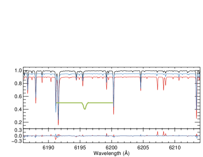
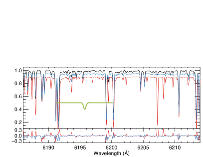
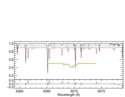
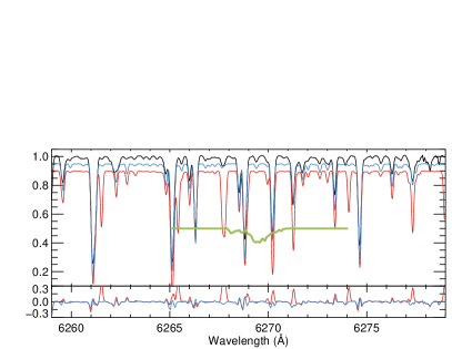
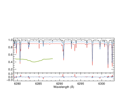
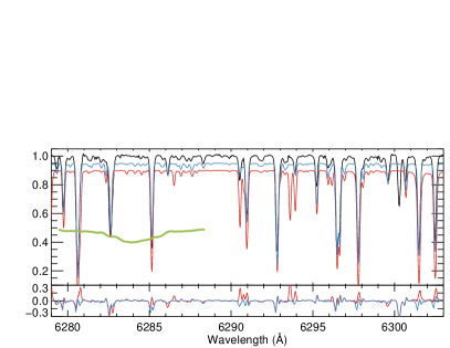
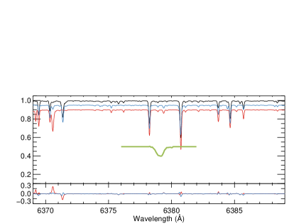
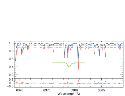
Figure 1: Comparison of the modeled spectra of the Sun (left) and Arcturus (right). Each pannel contains two graphics. In the main (upper) one, black line indicates the observed spectrum. Red and blue lines have been utilized to show the modeled spectrum using the original and improved line list, respectively. Note that for the shake of clarity these two lines have been offset by $-0.10$ and $-0.05$ in the y-axis. In the complementary (lower) one, the residuals (data - model) using both line lists are shown. Finally, the profiles for the DIBs that motivated the corrections presented here and a putative cloud at $v=0$ km s^-1 are included for reference.

2.3 Studied spectral ranges

In this contribution we focus on the spectral ranges of a reduced but relevant set of DIBs. As starting point, we used the list of DIBs presented in Tab. 1 of Puspitarini et al. (2013) and restricted to those DIBs included in the spectral range used by the Gaia-ESO survey to observe bright late-type stars. Specifically, this survey uses for this purpose the UVES spectrograph in its DIC1/580 nm setting, covering from 4760 Å to 6840 Å. Additionally, we required them to be relatively strong. That means having not only large equivalent width (EW) but also small full width at half maximum (FWHM). Using the results by Hobbs et al. (2008) for HD 204827 as reference, we restricted to those DIBs with EW(mÅ)/FWHM(Å)$>$60. Also, a good pre-existing model of the DIB profile is needed. We used the templates empirically derived by Raimond et al. (2012) and Puspitarini et al. (2013) who averaged several FEROS (R$\sim$48000) spectra of early-type (B-A5) stars. Because of their empirical nature, they take into account possible asymmetries in bands and/or blending with neighboring ISM features. We excluded $\lambda$6445.3 since the model needed further improvements (see Fig. 6. in Puspitarini et al., 2013). In this way, the final list of DIBs of interest includes $\lambda$6196.0, $\lambda$6269.8, $\lambda$6283.8, $\lambda$6379.3, and $\lambda$6613.6. For typical ISM velocities this last feature is strongly blended with a set of stellar lines at $\lambda$6614.4 Å  (Fe i) and 6613.7 Å  (Fe i and Y ii) particularly difficult to reproduce with the simple strategy described in Sec. 3. Therefore, we decide not to consider it at this stage and envision a more refined strategy for this range in the future. Finally, the fitting procedure needs some continuum towards the blue and red of the DIB under analysis and DIBs trace ISM at a certain velocity (and therefore can appear blue and red-shifted in the spectra). Taken all this into account, the following three spectral ranges were selected for inspection: 6 186-6 214 Å, 6 259-6 303 Å, 6 369-6 389 Å.

The first spectral range is also needed when analysing the $\lambda\lambda$6203.0,6204.5 blend. This is particularly interesting since the relative intensities of the DIBs in the blend do not vary in accord, pointing towards a different origin (Porceddu et al., 1991). Since these two DIBs did not fulfill our criterion of EW(mÅ)/FWHM(Å) ($\lambda$6204.5 is particularly broad), they will not be tested here. However, we note that studies on this blend based on late-type star spectra may equally benefit from the line list provided here.

Also, it is worth to note that the second spectral range is infested with a series of strong absorption telluric features between $\sim$6275 Å  and $\sim$6303 Å  caused mainly by O₂ in the atmophere (but also water vapor). Before tuning the stellar line list, the spectra of the Sun and Arcturus were corrected from this telluric absorption using TAPAS (Bertaux et al., 2014).

Table 3: Residual statistics for the Sun and Arcturus.

		The Sun		Arcturus
Range (Å)		$\mu\pm\sigma$	Median	$\mu\pm\sigma$	Median
6 186-6 214	O	-0.003$\pm$0.021	-0.004	0.001$\pm$0.071	-0.007
	U	-0.007$\pm$0.012	-0.005	-0.020$\pm$0.036	-0.010
6 259-6 279	O	0.008$\pm$0.034	0.003	0.013$\pm$0.078	-0.001
	U	-0.001$\pm$0.017	0.002	-0.013$\pm$0.032	-0.003
6 279-6 303	O	0.005$\pm$0.029	0.004	0.001$\pm$0.065	0.001
	U	0.000$\pm$0.014	0.003	-0.016$\pm$0.048	-0.002
6 369-6 389	O	-0.003$\pm$0.024	-0.003	-0.007$\pm$0.038	-0.010
	U	-0.004$\pm$0.010	-0.003	-0.011$\pm$0.017	-0.008

Table 4: List of modified stellar lines in the $6186-6214$ Å spectral range.

Ion	$\lambda_{ori}$	$\lambda_{new}$	$\log(gf)_{ori}$	$\log(gf)_{new}$
	(Å)	(Å)
Si i	6194.416	…	-2.076	-1.800
Si i	6194.884	…	-2.192	-2.400
Si i	6195.433	…	-1.490	-1.700
Si i	6208.541	…	-1.467	-2.000
Ca i	6204.757	…	-0.276	-2.000
Sc i	6193.666	…	-2.760	-10.000
Sc i	6210.658	6210.648	-1.529	…
Ti i	6186.141	…	-1.270	-1.650
Ti i	6200.318	…	-2.300	+0.300
Ti i	6200.227	…	-3.035	-2.450
V i	6188.961	6188.940	-1.062	-2.650
V i	6189.364	6189.342	-2.970	-2.700
V i	6190.495	…	-2.377	-2.600
V i	6199.197	6199.177	-1.300	-1.500
V i	6207.272	…	-1.370	…
V i	6213.866	6213.846	-2.050	-1.850
Fe i	6187.398∗	…	-4.148	-4.700
Fe i	6187.989∗	…	-1.720	-2.600
Fe i	6190.398	…	-1.520	-2.200
Fe i	6191.558∗	6191.563	-1.417	-1.700
Fe i	6196.968	…	-2.233	-2.800
Fe i	6198.042	…	-2.049	-2.400
Fe i	6199.506∗	…	-4.430	-4.975
Fe i	6200.312	6200.302	-2.437	-2.900
Fe i	6202.305	…	-5.191	-5.650
Fe i	6205.585	…	-2.219	-3.500
Fe i	6207.230	…	-1.969	…
Fe i	6208.211	…	-1.139	-2.500
Fe i	6209.714	…	3.249	-3.800
Fe i	6212.013	…	-4.758	-3.300
Fe i	6212.099	…	-2.913	-3.400
Fe i	6213.429	6213.419	-2.482	-2.900
Fe ii	…	6187.996	…	-4.800
Fe ii	…	6199.190	…	-3.941
Co i	6188.996	…	-2.450	-2.500
Co i	6197.833	…	-0.510	-1.200
Ni i	6191.178	6191.168	-2.939	-2.300
Ni i	6204.600	…	-1.100	-1.060
Y i	6191.718∗	…	-0.680	…
Nd ii	6210.680	6210.660	-1.540	-1.540

Table 5: Modified stellar lines in the $6259-6303$ Å spectral range.

Ion	$\lambda_{ori}$	$\lambda_{new}$	$\log(gf)_{ori}$	$\log(gf)_{new}$
	(Å)	(Å)
Si i	6279.343	…	-2.434	-1.700
Si i	6290.792	…	-1.074	-2.800
Si i	6299.599	…	-1.658	-1.200
Sc i	6276.295	…	-2.605	-2.720
Sc ii	6279.753	…	-1.252	-1.430
Ti i	6261.099	6261.089	-0.530	-0.470
Ti i	6266.010	…	-1.950	-2.150
Ti i	6268.525	…	-2.260	-2.200
Ti i	6273.388	…	-4.008	-4.180
Ti i	6293.004	…	-3.100	-3.000
Ti i	6295.248	…	-4.242	-4.290
Ti i	6296.646	…	-3.582	-3.650
V i	6266.307	…	-2.290	-2.090
V i	6268.798	…	-2.128	-2.000
V i	6274.649	…	-1.670	-1.620
V i	6285.150	…	-1.510	-2.200
V i	6296.487	…	-1.590	-1.790
V ii	6261.087	…	-2.389	-2.189
Fe i	6261.534	…	-1.004	-2.800
Fe i	6265.132	6265.127	-2.550	-2.750
Fe i	6265.422	6265.423	-0.975	-3.000
Fe i	6267.676	…	-2.759	-5.000
Fe i	6267.766	…	-1.363	-2.500
Fe i	6267.825	…	-2.376	-6.000
Fe i	6268.942	6268.932	-1.527	-2.900
Fe i	6270.224	6270.214	-2.464	-2.900
Fe i	6271.278	6271.268	-2.703	-3.150
Fe i	6274.089	…	-1.325	-2.400
Fe i	6277.334	…	-4.001	-4.300
Fe i	6277.530	6277.529	-4.651	-4.520
Fe i	6278.966	…	-1.139	-2.900
Fe i	6280.770	…	-1.659	-2.300
Fe i	…	6282.558	…	-1.800
Fe i	…	6282.760	…	-1.400
Fe i	6286.133	6286.130	-3.086	-3.200
Fe i	6286.509	…	-3.447	-4.330
Fe i	6288.323	…	-3.845	-2.900
Fe i	6290.543	…	-4.330	-4.875
Fe i	6293.611	…	-1.156	-2.700
Fe i	6293.924	…	-1.717	-2.150
Fe i	6296.180	…	-2.094	-2.600
Fe i	6297.792	…	-2.740	-3.000
Fe i	6301.500	…	-0.718	-1.200
Fe i	6302.494	…	-0.973	-1.300
Fe ii	6269.959	…	-4.500	-4.800
Fe ii	…	6286.130	…	-2.800
Fe ii	…	6301.500	…	+0.400
Fe i	6380.743	…	-1.376	-1.750
Co i	6262.829	…	-2.644	-2.800
Co i	6273.004	…	-1.035	-1.400
Ni i	6259.595	…	-1.237	-1.300
La ii	6262.290	…	-1.220	-1.500

Table 6: Modified stellar lines in the $6369-6389$ Å spectral range.

Ion	$\lambda_{ori}$	$\lambda_{new}$	$\log(gf)_{ori}$	$\log(gf)_{new}$
	(Å)	(Å)
Si i	6370.574	…	-0.947	-1.900
Si i	6380.689	…	-2.733	-1.400
Si ii	6371.371	…	-0.040	-0.150
Ca i	6374.930	…	-0.525	-1.500
Sc i	6378.807	…	-2.420	-2.625
Ti i	6371.496	…	-1.940	-1.900
Ti i	6374.321	…	-3.359	-0.700
V i	6379.364	…	-0.995	-1.995
V i	6384.445	…	-0.804	+0.800
Fe i	6369.217	…	-2.344	-4.300
Fe i	6376.201	…	-2.928	-3.440
Fe i	6380.743	…	-1.376	-1.750
Fe i	6383.708	…	-2.644	-3.100
Fe i	6385.718	…	-1.910	-2.200
Fe i	6388.405	…	-4.476	-4.270
Fe ii	6369.459	…	-4.231	-4.450
Ni i	6370.346	…	-1.940	-1.890
Ni i	6378.247	…	-0.830	-0.900
Sr i	6388.199	…	-1.070	+0.000

3 Towards an optimized line list

The stellar line list was improved by comparing synthetic spectra with the observed spectra for the Sun and Arcturus described in Sec. 2.1. For that, we utilized the radiative transfer code TURBOSPECTRUM (Alvarez & Plez, 1998; Plez, 2012) that requires a model with the stellar atmosphere structure. For the Sun, we utilized one of the native models from the grid of MARCS models for late-type stars (Gustafsson et al., 2008) while for Arcturus, we interpolated using a code provided by T. Masseron. Additionally, basic stellar parameters as well as the geometry of the atmosphere needed to be provided. Utilized parameters for both stars are listed in Tab. 2. The last input for TURBOSPECTRUM is a list with the physical parameters of the lines that we intend to tune. We used as starting point those provided by the Vienna Atomic Line Database (VALD-3) (Ryabchikova et al., 2015). With this, two initial synthetic spectra were created and degraded to an effective resolution that takes into account the broadening due to rotation and turbulence of the stars. Utilized values are showed in the last column of Tab. 2.

The synthetic spectra using TURBOSPECTRUM and the original VALD-3 line list are shown in Fig. 1 in red. A quick inspection of this Figure is enough to state that several spectral features are not properly modeled with residuals with absolute values $\hbox{\hbox to0.0pt{\lower 2.36806pt\hbox{$\sim$}\hss} \kern-3.00003pt\raise 1.72218pt\hbox{$>$}}10$% . In most of those cases, equivalent width of the stellar line is overestimated. Some examples have already been noticed (see e.g. a residual at $\sim$6609.5 Å  in Fig. 2 of Puspitarini et al., 2015).

We modified the VALD-3 line list with the esprit of keeping the tuning as simple as possible. Thus, we allowed ourselves to modify only the oscillator strength ($\log(gf)$) and, exceptionally, the wavelength of the line. In those few cases where no line responsible for a given feature was identified, we created a new line by replicating a nearby Fe I or Fe II line at the wavelength of the feature that we intend to reproduced. This is reasonable strategy, since iron lines are ubiquitous and iron is good proxy for the star metallicity. Finally, in those cases where a different $\log(gf)$ was required to minimize the residuals for the Sun and for Arcturus, we adopted an intermediate value for $\log(gf)$ as a compromise. This is a pragmatic approach valid for our goals (i.e. get rid out of the stellar spectra, without necessarily having a deep understanding of the stellar physics). Synthetic spectra using TURBOSPECTRUM and our modified line list are shown in blue in Fig. 1. Even if there are still some low-level residuals, typically $\sim$ $<$10%, these synthetic spectra clearly beat those created with the TURBOSPECTRUM code together with the original VALD-3 line list.

Table 3, that contains the means, standard deviations and medians of the residuals in each subplot of Fig. 1, offers a more quantitative way of comparing all the three options. By looking at the standard deviations of the residuals, it is clear that TURBOSPECTRUM models using the updated line list are much better than those using the original one. Since the residuals that matter most are those within the relatively narrow wavelength ranges that include only each DIB itself plus some limited continuum to either side, we also estimated the local standard deviation, in 2 Å-wide bins, for both the Sun and Arcturus. As it happened with the global standard deviations, these were comparable or smaller when using the updated line list than when using the original ones.

The updated line lists are the main outcome of this contribution and they are offered to the community in Tables 4 to 6. In the following section, we will show some examples of its applicability for DIB extraction.

4 DIB extraction using the new line list

Table 7: Stellar parameters for the test stars.

Star	$T_{eff}$	$\log g_{spec}$	$\xi_{turb}$	[Fe/H]	Ref.
	(K)	(cm s-2)	(km s-1)
NGC 2682 San1092	6074.	4.39	1.35	+0.04	S09
NGC 2682 San1048	5915.	4.48	0.96	+0.07	S09
NGC 2682 No164	4812.	2.73	1.57	+0.03	S09
NGC 2682 No266	4862.	2.76	1.59	+0.01	S09
IC 4651 AMC1109	6075.	4.54	1.14	+0.15	S09
IC 4651 AMC4226	5862.	4.31	0.89	+0.13	S09
NGC 6705 No1111	5039.	2.85	2.18	+0.14	S12
NGC 6705 No1184	4518.	2.09	1.92	$-$0.01	S12

Table 8: DIB measurements for the test stars.

6196.0

6269.8

6283.8

6379.3

Star

EW

$v$

$\chi^{2}$

EW$\pm$e(EW)

$v$

$\chi^{2}$

EW

$v$

$\chi^{2}$

EW

$v$

$\chi^{2}$

(mÅ)

(km s-1)

(mÅ)

(km s-1)

(mÅ)

(km s-1)

(mÅ)

(km s-1)

NGC2682 San1092

O

$<10$

…

0.81

$<28$

…

1.00

$182\pm 18$

$-9\pm 5$

1.61

$<16$

…

1.19

U

$<9$

…

0.79

$<21$

…

0.66

$120\pm 15$

$+19\pm 7$

1.35

$<11$

…

0.50

NGC2682 San1048

O

$<20$

…

2.78

$<72$

…

6.19

$<194$

…

4.73

$<27$

…

2.82

U

$<20$

…

2.72

$<69$

…

5.67

$<180$

…

4.23

$<25$

…

2.34

NGC2682 No164

O

$23\pm 17$

$-4\pm 2$

0.96

$<47$

…

2.72

$243\pm 93$

$+13\pm 7$

3.96

$<14$

…

0.90

U

$14\pm 11$

$-4\pm 3$

0.82

$<22$

…

0.65

$125\pm 73$

$+12\pm 8$

1.53

$<10$

…

0.49

NGC2682 No266

O

22$\pm$16

$-4\pm 2$

0.81

$<45$

…

2.51

$251\pm 79$

$+9\pm 6$

3.57

$<14$

…

0.88

U

14$\pm$10

$-5\pm 3$

0.70

$24\pm 20$

$-19\pm 4$

0.60

$158\pm 84$

$+9\pm 6$

1.82

$<10$

…

0.48

IC 4651 AMC1109

O

16$\pm$2

$-15\pm 2$

0.53

$<30$

…

1.19

$265\pm 38$

$+9\pm 3$

1.63

$19\pm 3$

$-15\pm 2$

0.33

U

17$\pm$2

$-15\pm 2$

0.37

$31\pm 18$

$-18\pm 2$

0.41

$189\pm 9$

$+1\pm 5$

0.70

$19\pm 2$

$-16\pm 2$

0.32

IC 4651 AMC4226

O

12$\pm$3

$-17\pm 3$

0.67

$<31$

…

1.19

$75\pm 15$

$-60\pm 16$

2.75

$13\pm 3$

$-16\pm 3$

0.42

U

12$\pm$3

$-16\pm 3$

0.55

$23\pm 11$

$-26\pm 3$

0.51

$203\pm 9$

$-28\pm 4$

1.09

$13\pm 3$

$-18\pm 3$

0.40

NGC6705 No1111

O

29$\pm$13

$-24\pm 2$

1.90

$46\pm 37$

$-33\pm 4$

4.17

$804\pm 51$

$-45\pm 2$

4.45

$79\pm 9$

$-18\pm 1$

1.99

U

36$\pm$10

$-22\pm 1$

1.94

$77\pm 18$

$-28\pm 2$

1.60

$736\pm 74$

$-45\pm 2$

2.44

$87\pm 7$

$-19\pm 1$

1.69

NGC6705 No1184

O

26$\pm$8

$-24\pm 2$

2.47

$78\pm 6$

$-37\pm 13$

4.25

$810\pm 67$

$-46\pm 2$

4.75

$83\pm 15$

$-19\pm 1$

1.49

U

34$\pm$12

$-23\pm 2$

2.66

$115\pm 44$

$-43\pm 2$

2.23

$712\pm 111$

$-44\pm 2$

3.14

$101\pm 20$

$-18\pm 1$

1.58

Dwarf stars                                                                             Giant stars

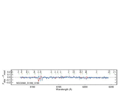
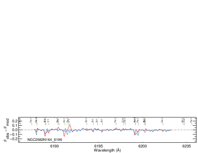
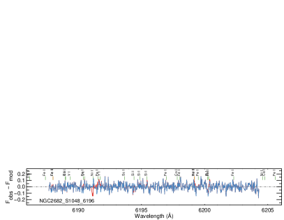
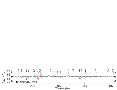
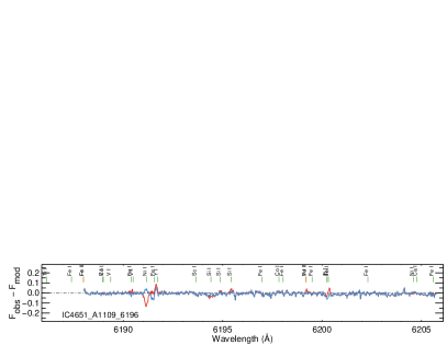
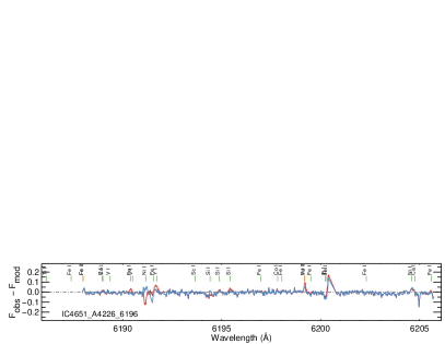
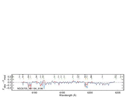
Figure 2: Comparison of the fit residuals for the DIB at $\lambda$6196.0 Å. Dwarf test stars are on the left column, while giant stars are on the right. We used red lines for the synthetic spectra using the original line list and blue lines for those with the improved one, as in Fig. 1.

Dwarf stars                                                                             Giant stars

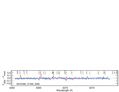
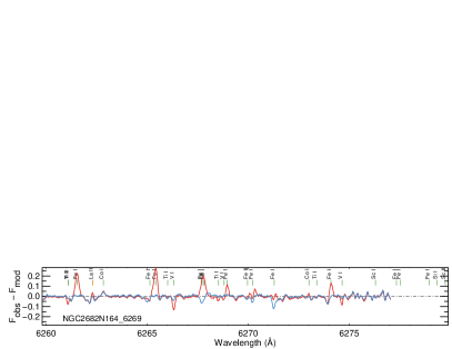
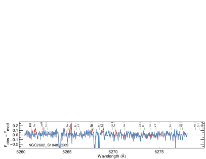
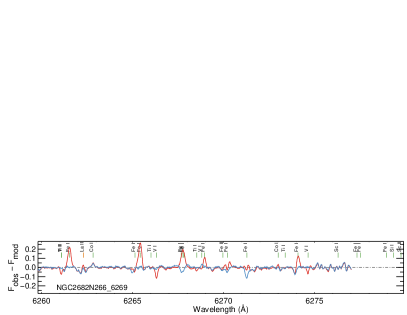
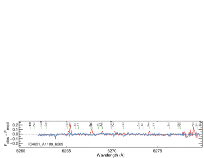
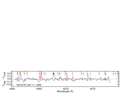
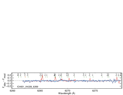
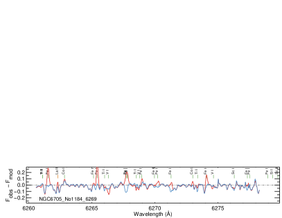
Figure 3: Same as for Fig. 2 but for the DIB at $\lambda$6269.8 Å.

Dwarf stars                                                                             Giant stars

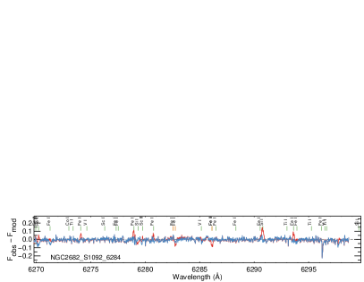
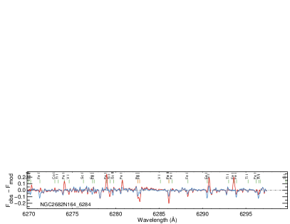
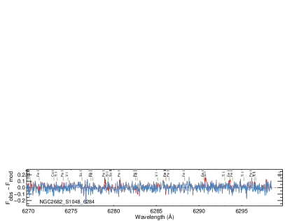
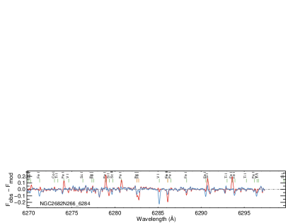
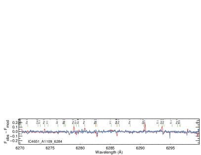
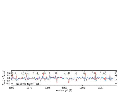
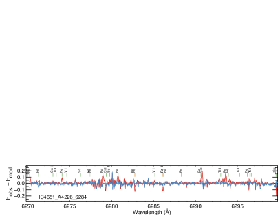
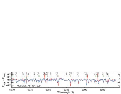
Figure 4: Same as for Fig. 2 but for the DIB at $\lambda$6283.8 Å.

Dwarf stars                                                                             Giant stars

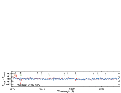
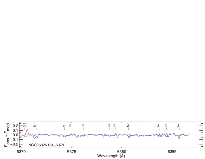
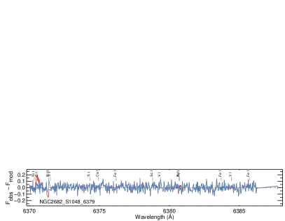
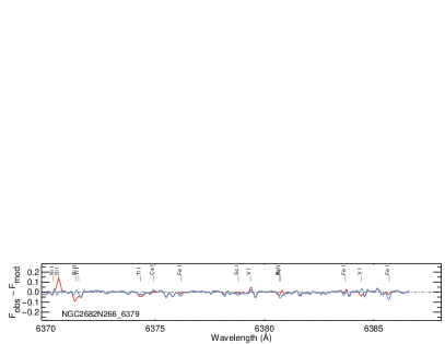
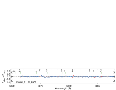
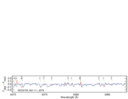
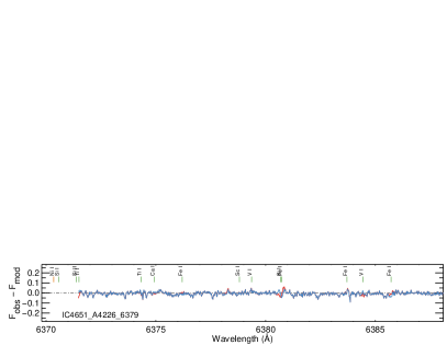
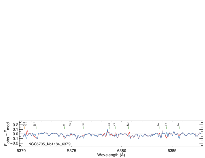
Figure 5: Same as for Fig. 2 but for the DIB at $\lambda$6379.3 Å.

We tested our updated line lists using the UVES spectra presented in Sec. 2.2. A thorough description of the strategy to measure the DIB equivalent widths can be found in Puspitarini et al. (2013) and Monreal-Ibero et al. (2015a) and will not be repeated here. In short, the spectra are modeled as the product of a series of functions that reproduce the stellar absorption features, the stellar global continuum, the interstellar absorption (i.e. the DIB), and the telluric transmission. DIBs were expected to be weak, specially along the sight-lines with low reddening. Thus, additional constrains were needed to make the fits converge. Specifically, we impose limits on the expected velocities for the DIBs, based on the direction of the sky and on the results for H i  (Brand & Blitz, 1993; Kalberla et al., 2010). Each UVES spectrum was fitted twice. The only brick that we changed in these two fits was the function representing the stellar absorption features. In both cases we used TURBOSPECTRUM to create the synthetic stellar spectrum but using either the original VALD-3 stellar line lists or including our updates. The identical stellar parameters that we used to create both models are listed in Table 7. Also, we set [$\alpha$/Fe]=0.0 and we assumed a plane-parallel geometry for the dwarf stars, and a spherical geometry for the giants.

The derived DIB parameters, both equivalent width and velocity, for the eight test spectra are presented in Table 8. Reported errors for the equivalent widths take into account two components. The first one is the formal 1-sigma statistical errors associated to the fit. The second one is an estimation of the uncertainty associated to the reported stellar parameters ($T_{eff}$, $\log g$, and metallicity). For that, in those cases where the band could be strongly blended with a strong stellar line, the fit was done two times: without any mask, and masking this contaminating line. The difference between the equivalent widths derived from these two fits is an estimation of the uncertainty due to that, and as such, was added to the error budget. In those cases where the fit did not converge (i.e. the estimated DIB velocity reached the imposed limits), we estimated an upper limit for a possible DIB using the standard deviation of the residuals and the typical width of the DIB. Regarding the reported errors in the velocities, these include only the formal 1-sigma statistical errors associated to the fit.

The most relevant result that one can extract from Table 8 is that the $\chi^{2}$ is most of the times smaller when using the synthetic spectra generated with the new line list, supporting the use of the corrections provided in Sec. 3. Besides, even in the few cases where the $\chi^{2}$ is comparable, lines in the proximity of the DIB are better reproduced when using the improved line list and only a few lines at the edge of the spectral range under consideration are have relatively important residuals. This is visualized in a graphical manner in Figures 2 to 5 that display the residuals for the fits of the eight stars when using the original (red) and updated (blue) line lists. These last ones are $\hbox{\hbox to0.0pt{\lower 2.36806pt\hbox{$\sim$}\hss} \kern-3.00003pt\raise 1.72218pt\hbox{$<$}}0.1$ for the dwarf star spectra. Regarding the giant stars, only for a few lines in the spectral range of the DIB at $\lambda$6196.0 they are slightly larger than 0.1. These lines are particularly susceptible to further improvements and have been marked in Table 4 with an asterisk. The determination of the $\log(gf)$ and the central wavelength can change depending on the stars used for calibration (e.g. convection inside the star may have an effect on the central wavelength of a given stellar line, see Molaro & Monai, 2012). Thus, small additional adjustments in both $\log(gf)$ and the central wavelength using additional calibration stars can further improve the modeling of these lines.

Not every DIB was detected in every spectrum. This is not surprising, given the covered range of stellar extinctions (see Tab. 1). The DIB that was detected in a larger number of spectra is that at $\lambda$6283.8. The derived equivalent widths are smaller when using the up-dated line list in all cases but IC4651AM4226. This is very much in line with the result by Kohl et al. (2016) for the DIB at $\lambda$5780 who, after carefully quantifying the stellar absorption in some spectra with previously reported ISM absorption, did not find hints of DIB detection and highlight the importance of adequately reproducing the stellar spectrum.

The other DIBs were only detected in some of the stars. To have an idea of the relative importance of all the different components playing a role (different ISM absorptions, stellar spectrum, etc.) we show the fits for the four DIBs in NGC6705_No1111 in Figure 6. Note that this is both a giant and a relatively high-metallicity star. This implies that stellar absorptions are particularly strong here, and thus this is representative of one of the most difficult examples that one might find in a putative future exploitation of MOS spectra for ISM studies. All these points are equally applicable to the other star in the cluster, NGC6705_No1184. In particular, the fitting algorithm was able to identify an excess of absorption at the position for the DIB at $\lambda$6269. However, this line is strongly blended with three stellar lines at $\sim\lambda 6268$ (Ti I, V I, Fe i), which might prevent an accurate determination of the DIB centroid (i.e. velocity) and explain the differences in velocity with respect to he DIB at $\lambda$6283.8. Alternatively, small uncertainties in the automatic reduction of the archive data by the ESO pipeline (e.g. local issues with flat-fielding, fringing) could play a role in the determination of the centroid of large features, as is the case of the DIB at $\lambda$6283.8. A final source of uncertainty, regarding the velocities, is the structure in velocity for the ISM itself along the line of sight. Since our goal here is testing the line list, not the fitting technique, we used the simple approach of reproducing the ISM absorptions by one single component (i.e. one cloud). However, this is not necessarily true. For example, in the direction of NGC 6705, H i  observations show at least the existence of two clouds at very different velocities (Kalberla et al., 2010). The simplicity of a fit using only one component coupled with differences in the physical conditions between these clouds might also explain the velocities differences observed between the different DIBs.

All in all, the line list corrections provided here offer the possibility of making better use of the colossal amount of cold star spectra generated in the forthcoming years for DIB research. From the technical point of view, the most promising DIB, is the one at $\lambda$6283.8. Armed with a good fitting algorithm, an accurate synthetic stellar spectrum (as the one that can be generated using this updated line list) and appropriate tools for good telluric corrections, like TAPAS here, but also e.g. Molecfit (Smette et al., 2015), researchers will be able to extract plenty of material that will help to constrain the structure of the Galactic ISM. However, given the dependence of this DIB with the environment, additional information coming from e.g. other DIBs will be desirable, and certainly feasible in the light of sights with higher extinction.

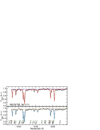
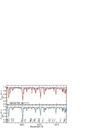
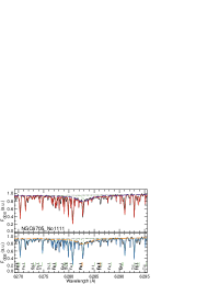
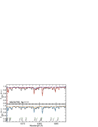
Figure 6: NGC6705_No1111 as example of fit in the spectral region for each DIB. Total spectra are represented with solid lines as follows: black - observed spectra; red - fit with original line list; blue - fit with updated line list. Components associated to the modeled DIBs are displayed with long-dashed violet and orange lines while the synthetic spectra as created by TURBOSPECTRUM appear as green short-dashed lines.

5 Summary and conclusions

In this paper we improve the extraction of the parameters associated to the DIBs in the spectra of cool stars by providing updated line lists in three spectral ranges associated the four strong DIBs at $\lambda$6196.0, $\lambda$6269.8, $\lambda$6283.8, and $\lambda$6379.3. For that we tuned the $\log(gf)$ (and occasionally the central wavelength) of the stellar lines and created synthetic spectra with TURBOSPECTRUM for the Sun and Arcturus, that minimized the residuals for both stars when comparing synthetic and observed spectra.

The final stellar synthetic spectra with the improved line lists reproduce the observed spectra for these stars with greater accuracy. The global standard deviation for the residual in a given spectral range when using TURBOSPECTRUM with the updated line lists are typically about half of those using the original lists, and with local residuals $\sim$ $<$10%, for both stars. We tested our updated line list with a set of UVES spectra for eight stars both, dwarf and giants, and suffering from different amount of extinction. The quality of the fit, as characterized by the $\chi^{2}$, was better when using our updated line lists, and thus we offer them to the community.

Despite the general improvement of the models, discrepancies between the radial velocities measured for the $\lambda$6283.8 DIB and for the other DIBs remain. However, based on a similar fitting method radial velocities were consistently measured in the spectra of the ESO-Gaia Survey at high optical extinctions ($A_{V}\sim 1$  mag, see Figs. 8, 9, 12, 14 and 16 by Puspitarini et al., 2015). The examples chosen here (lower extinction towards metallic giant stars) are much more challenging and our results strongly suggest that additional work needs to be done either to improve the updated atomic data, and/or the profiles of the theoretical stellar lines to reach the high degree of precision (a few percent) that will allow to derive reliable radial velocity in these more challenging cases.

Here, we have focused on the improvement of the stellar modeling in three specific spectral ranges, corresponding to four strong DIBs. Inaccuracies in the stellar atmospheric modeling have already identified in other spectral ranges of interest for ISM research, as the one associated to the DIBs at $\lambda$5780 and $\lambda$5797 (Kohl et al., 2016). Given the value of the ratio between these two DIBs as a tracer of the characteristics of the environment (i.e. radiation field) (Cami et al., 1997; Vos et al., 2011; Cordiner et al., 2013), there is a strong motivation for a similar work to the one presented here for this spectral range. Likewise, the DIB at $\lambda$6614 is relatively strong and, as such, the creation of synthetic spectra in this spectral range should be contemplated, though a preliminary exploration of this range, not discussed here, points towards a need for a more delicate approach, where for some stellar lines, additional parameters other than $\log(gf)$ should be tuned and/or effects like departures form LTE, explored. These updated line lists together with the enormous data base that will be generated in the forthcoming years will offer an extraordinary opportunity to learn about the nature, and statistical properties of DIBs. Likewise, their suitability as probes of the properties of the ISM (e.g. distribution, excitation, etc.) will be significantly enhanced. In particular, the assigned value for the foreground extinction affects the determination of the stellar parameters (e.g. effective temperature, metallicity). DIBs, with their capacity to act as independent estimators of the extinction, will play a fundamental role in constraining this value.