Polarization and long-term variability of Sgr A* X-ray echo

Abstract

We use a model of the molecular gas distribution within $\sim 100$ pc from the centre of the Milky Way (Kruijssen, Dale & Longmore) to simulate time evolution and polarization properties of the reflected X-ray emission, associated with the past outbursts from Sgr A^∗. While this model is too simple to describe the complexity of the true gas distribution, it illustrates the importance and power of long-term observations of the reflected emission. We show that the variable part of X-ray emission observed by Chandra and XMM-Newton from prominent molecular clouds is well described by a pure reflection model, providing strong support of the reflection scenario. While the identification of Sgr A^∗ as a primary source for this reflected emission is already a very appealing hypothesis, a decisive test of this model can be provided by future X-ray polarimetric observations, that will allow placing constraints on the location of the primary source. In addition, X-ray polarimeters (like, e.g., XIPE) have sufficient sensitivity to constrain the line-of-sight positions of molecular complexes, removing major uncertainty in the model.

1 Introduction

Several molecular complexes in the central $\sim 100$ pc of the Milky Way are not only prominent IR or submm sources, but they are also bright in X-rays (see, e.g., Genzel, Eisenhauer, & Gillessen, 2010, for review). Their spectra have several features characteristic for X-ray reflection by cold gas. It was suggested that Sgr A^∗ (a supermassive black hole at the centre of the Galaxy) is responsible for the illumination of these clouds (e.g., Sunyaev, Markevitch, & Pavlinsky, 1993; Markevitch, Sunyaev, & Pavlinsky, 1993; Koyama et al., 1996). This suggestion implies that Sgr A^∗, despite its present-day low luminosity (see, e.g., Yuan & Narayan, 2014, for review), was much brighter few hundred year ago. Since then, the problem of clouds illumination has been subject to many theoretical and observational studies (see Ponti et al., 2013, for review). One of the specific predictions of the illumination/reflection scenario is that the continuum emission is polarized (Churazov, Sunyaev, & Sazonov, 2002). The polarization can not only constrain the position of a primary source illuminating a given cloud (from the orientation of the polarization plane), but also the position of the cloud along the line of sight (from the degree of polarization).

There were many studies that consider the reflection scenarios in the GC region (e.g., Sunyaev & Churazov, 1998; Murakami et al., 2000; Clavel et al., 2014; Molaro, Khatri, & Sunyaev, 2016; Marin et al., 2015). Here we return to this problem to emphasize the power of long-term monitoring of the reflected emission. We illustrate this point by using models of the molecular gas distribution in the central $\sim$100 pc around Sgr A^∗ (e.g., Molinari et al., 2011; Kruijssen, Dale, & Longmore, 2015; Henshaw et al., 2016; Ginsburg et al., 2016; Schmiedeke et al., 2016) to calculate the expected reflected signal over few hundred years. Even although the true distribution of the gas is likely more complicated than prescribed by these models (see Churazov et al., 2017), this exercise shows that mapping molecular gas by X-ray observations will eventually lead to a clear 3D picture of the central molecular zone. We show that new X-ray polarimetry missions that are currently under study by ESA and NASA (e.g., Soffitta et al., 2013; Weisskopf et al., 2013) have sufficient sensitivity to make a decisive contribution in resolving the ambiguity in the position of molecular clouds along the line of sight, and consequently confirm or reject the identification of Sgr A^∗ as a primary source of the illumination (see also Marin et al., 2015).

Throughout the paper we assume the distance to Sgr A^∗ $R_{0}=8~{}{\rm kpc}$ (see, e.g., Genzel, Eisenhauer, & Gillessen, 2010, for discussion of different distance indicators), therefore $1^{\prime}$ corresponds to 2.37 pc.

2 Spherical cloud illuminated by a steady source

We first consider a simple case of a uniform spherical cloud illuminated by a steady source and we perform full Monte Carlo simulations of the emergent spectrum, taking into account multiple scatterings, similar to Churazov et al. (2008).

2.1 Illuminating source spectrum

We assume that the primary unpolarized X-ray source is located at a large distance from the cloud (much larger than the size of the cloud) and, therefore, the cloud is illuminated by a parallel beam of radiation, i.e. incoming photons are hitting a hemisphere facing the primary source (see Fig. 10 in Appendix A). The illuminating source has a power law spectrum with a photon index $\Gamma=2$, i.e., $I(E)=AE^{-\Gamma}~{}{\rm photons~{}s^{-1}~{}keV^{-1}}$, where $E$ is the photon energy. Since we are interested primarily in the reflected spectrum in the 1-10 keV band, the behavior of the spectrum at high energies is not very important for this study.

2.2 Radiative transfer

In modelling the radiative transfer, we followed the assumptions used in Churazov et al. (2008). In particular, we have included the following processes: photoelectric absorption, fluorescence, Rayleigh and Compton scattering. The abundance of heavy elements in the molecular gas is highly uncertain (e.g., Koyama et al., 2007). To model photoelectric absorption we used solar abundance of heavy elements from Feldman (1992), but set the abundance of iron to 1.6 solar (see, e.g., Nobukawa et al., 2010; Terrier et al., 2010; Mori et al., 2015). The cross sections for photoelectric absorption were taken from approximations of Verner & Yakovlev (1995) and Verner et al. (1996). For calculation of the fluorescent emission we used fluorescent yields from Kaastra & Mewe (1993). The fluorescent lines of all astrophysically abundant elements were included in the calculations and added to the corresponding bins of the scattered spectrum. The fluorescent photons are emitted isotropically without any net polarized. The modeling of the Rayleigh and Compton scattering employs differential cross-sections from the GLECS package (Kippen, 2004) of the GEANT code (Agostinelli et al., 2003) and the Klein-Nishina formula for free electrons. This model effectively accounts for effects of bound electron on the shape of the Compton shoulder of scattered fluorescent lines (see Sunyaev & Churazov, 1996; Vainshtein, Sunyaev, & Churazov, 1998), leading to a less sharp peak of the backscattered emission.

The photons coming from the direction of the primary source are absorbed or scattered in the cloud. A weight $w=1$ is assigned to each incoming photon. The evolution of each photon is traced for multiple scatterings inside the cloud, each time reducing the weight according to the probability of being absorbed or escape from the cloud after each scattering. The process stops once the weight drops below a certain threshold, in our case $w<10^{-8}$.

2.3 Model spectra

With the above assumption the emergent spectrum depends on two parameters: i) the optical depth of the cloud, parametrized via the Thomson optical depth of the cloud $\tau_{T}=\sigma_{T}n_{H}R$, where $n_{H}$ is the number density of hydrogen atoms and $R$ is the radius of the cloud, and ii) $\mu=\cos\theta$, the cosine of the angle $\theta$ between the direction of the primary beam and the line of sight (see Fig. 10 in Appendix A). In the code the total flux of the of incoming photons is normalised to unity (in ${\rm photons~{}s^{-1}~{}keV^{-1}}$) at 1 keV.

Typical simulated emergent spectra (as functions of $\tau_{T}$ and $\theta$) are shown in Fig. 1. For clarity each plotted spectrum is slightly shifted in energy. The left panel shows the variations of the observed spectrum with the optical depth of the cloud, when the angle between the line of sight and the primary beam is fixed at 90^∘. For small optical depth ($\displaystyle\tau_{T}=0.01$) the spectrum (the red line) has a shape resembling the shape of the incident spectrum (except at low energies, where photoelectric absorption strongly dominates Thomson scattering). As the optical depth increases the spectrum evolves towards a typical “reflection” spectrum from a semi-infinite medium. The right panel shows the variations of the spectrum with the viewing angle, while the optical depth is fixed to $\tau_{T}=0.5$. In this case, the scattering by $\sim$160^∘, i.e. back scattering, leads again to the spectrum resembling reflection from semi-infinite medium with a flat (and even slightly raising with energy) spectrum (the red line). In the small-angle scattering limit, i.e., we view a cloud illuminated from the back, the spectrum has a stronger decline at low energies, caused by the photoelectric absorption (the black line).

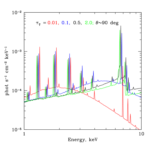
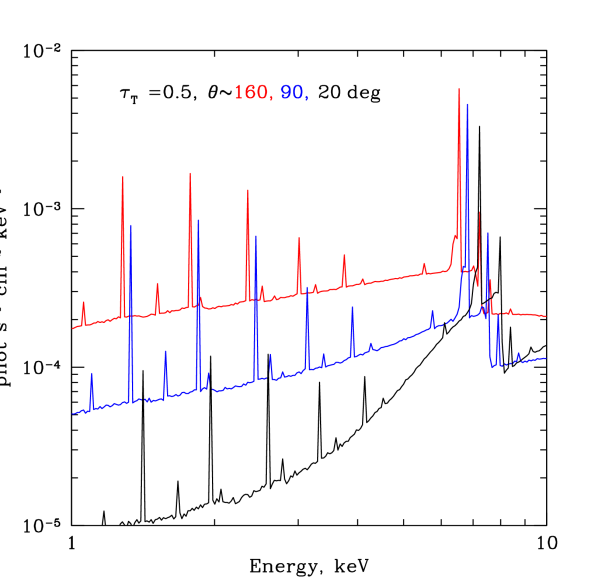
Figure 1: Typical spectra emerging from a spherical could illuminated by a distant source with a power law X-ray spectrum (see §2). Each plotted spectrum is shifted in energy for clarity. The most prominent fluorescent line is due to iron at $\sim$6.4 keV, while at lower energies the lines of Ca [3.7 keV], Ar [3.0 keV], S [2.3 keV], Si [1.7 keV] and Mg [1.2 keV] are visible, as well as few weaker fluorescent lines of less abundant elements. A “Compton shoulder” due to the scattered fluorescent photons is strong enough to be visible only for iron. Left: Dependence of the emergent spectrum on the optical depth of the cloud. The red, blue, black and green lines correspond to $\tau_{T}=0.01$, 0.1, 0.5 and 2, respectively. The angle between the line of sight and the primary beam is 90^∘​ for all spectra. For small optical depth ($\displaystyle\tau_{T}=0.01$) the spectrum (the red line) has a shape resembling the shape of the incident spectrum (except at low energies, where photoelectric absorption strongly dominates Thomson scattering). As the optical depth increases the spectrum evolves towards typical “reflection” spectrum from a semi-infinite medium. Right: Dependence of the emergent spectrum on the angle $\theta$ between the line of sight and the primary beam. The optical depth ($\tau_{T}=0.5$) is the same for all spectra. For $\theta\sim$160^∘(red line), i.e. back scattering, the spectrum resembles reflection from a semi-infinite medium. In the opposite limit $\theta\sim$20^∘, i.e., a cloud illuminated from the back, the spectrum has a strong decline at low energies, caused by the photoelectric absorption (black line).

In section §3 we use these spectra in application to the real data to single out the contribution of the reflected emission to the observed X-ray spectra in the GC region.

An XSPEC-ready model “CREFL16” based on §2.2 is publicly available (see Appendix A for a short description). The model covers 0.3-100 keV energy range. Apart from the normalization, the model has four parameters: radial Thomson optical depth of the cloud, slope of the primary power law spectrum, abundance of heavy elements and the cosine of the viewing angle. Compared to recently released model of Walls et al. (2016), the model includes fluorescent lines not only for iron, but for other elements too and has abundance of heavy elements (heavier than He) are a free parameter.

3 Hints from observations

Shown in Fig. 2 is the XMM-Newton EPIC-MOS $\sim 110^{\prime}\times 30^{\prime}$ image of the GC region in the 4-8 keV band. The image was accumulated over all publicly available observations in the archive. In this image, Sgr A^∗ is located in a red patch near to the centre of the image. In this section we will use the data from this $\sim 110^{\prime}\times 30^{\prime}$ ($\sim 260\times 70$ pc) area for spectral analysis of the diffuse emission and decomposition of the spectrum into two components (see also Ponti et al., 2015, for the corresponding emission in X-ray continuum and soft X-ray lines).

3.1 Contributions of the reflected and hot plasma components

For spectrum extraction we have selected four regions shown with black circles in Fig. 2. Three bigger circles cover regions known to be bright in the reflected radiation, from left to right: Sgr B2, the “Bridge” and Sgr C (see, e.g., Soldi et al., 2014). The resulting spectra, after excising contributions from bright point sources, are shown in Fig. 3 with black crosses. The fourth (smaller) circle is chosen, rather arbitrarily, to represent an example of X-ray bright region with a weak reflected component. All four spectra show two very prominent X-ray lines at 6.7 and 6.9 keV that have been identified with the lines of He-like and H-like ions of iron, produced by hot plasma (e.g., Koyama et al., 1989). Despite of the diffuse appearance of this component, it can, at least partly, be attributed to the emission coming from compact sources - accreting white dwarfs as in the Galactic Ridge (see Revnivtsev et al., 2009), while the fractional contribution of compact source may vary across the region considered here. The three spectra the from regions known to be bright in reflected emission, show, in addition, a very prominent line at $\sim$6.4 keV, corresponding to fluorescent emission of neutral (or weakly ionized) iron.

Assuming that the diffuse X-ray emission in the GC regions can be produced by the sum of hot plasma emission and reflected emission, we try to model the observed spectra as a linear combination of these two spectral templates. We reproduce the hot plasma component with the APEC model (Smith et al., 2001) of an optically thin plasma emission with a temperature fixed to 6 keV (e.g. Koyama et al., 2007). For the reflected component we have selected one of the simulated spectra of the reflected emission, namely the one corresponding to $\tau_{T}=0.5$ and the scattering angle of 90^∘. While these two templates are not able to describe the full complexity of the observed spectra, the hope is that over a limited energy range from $\sim$5 to $\sim$8 keV these two templates might capture essential signatures of both components. We therefore fit the observed spectra with the sum of these templates and we determine their normalizations, while keeping all other parameters fixed. We use:

$$S(E)=A_{1}R(E)+A_{2}P(E),$$ (1)

where $S(E)$ is the observed spectrum, $R(E)$ and $P(E)$ are the template spectra for the reflected component and for hot plasma emission, respectively, and $A_{1}$ and $A_{2}$ are the free parameters of the fit. The resulting fits are shown in Fig. 3. The red and blue lines show the reflected and hot plasma components and the green line shows the sum. Despite the simplicity of the model, the best fit can reproduce the essential features of the spectrum. For each of the three regions with a prominent reflection component the fit clearly shows that the reflected and hot plasma components contribute roughly equally to the continuum. Later, in §6, we will use this result in order to estimate the polarization of the total emission. Fig. 3 shows that for the forth region the quality of the fit is worse and the contribution of the reflected component is anyway small. We used this region only for the sake of a test, to compare with the results for three other regions.

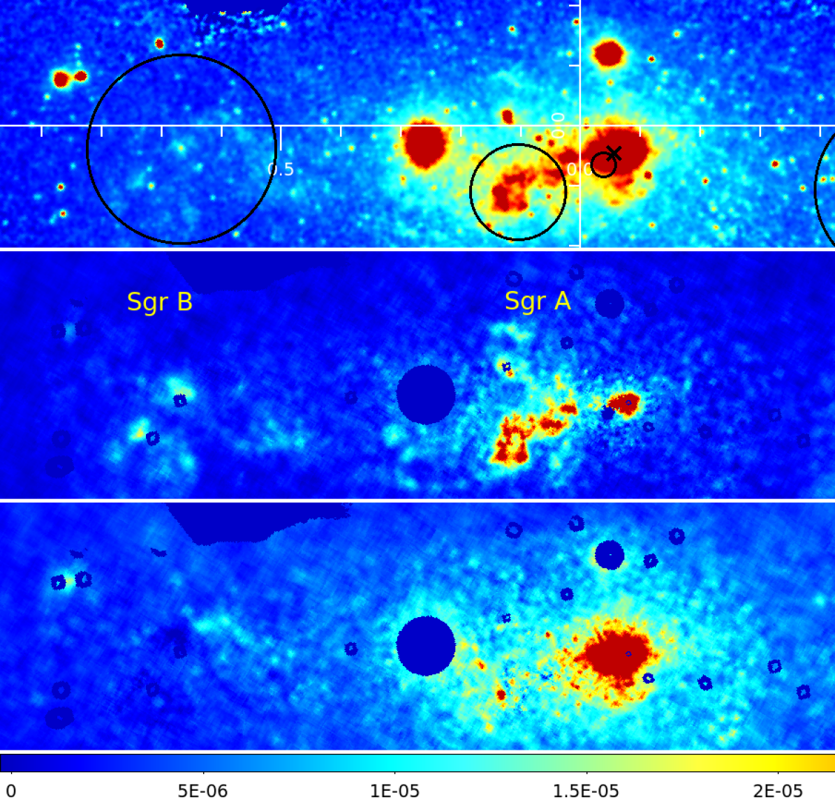
Figure 2: XMM-Newton maps ($\sim 110^{\prime}\times 30^{\prime}$) of the GC region in Galactic coordinates. The top panel shows the 4-8 keV map in units of ${\rm phot~{}s^{-1}~{}cm^{-2}~{}arcmin^{-2}}$; see colorbar at the bottom of the Figure. The position of Sgr A^∗ is marked with a black X in the top panel. Several very bright spots correspond to bright compact sources (X-ray binaries), which appear very extended in the image that is tuned to show faint diffuse emission. Note also, that scattering by dust grains could lead to extended halos around sources in the Galactic Center region (see, e.g., Jin et al., 2016, for the analysis of AXJ1745.6-2901 halo). The four black circles show the regions used for spectra extraction and analysis in §3.1. The three bigger circles correspond to the regions where the reflection component is known to be strong (e.g., Soldi et al., 2014). The smallest circle represents an example of an X-ray bright region with a weak reflected component. The lower two panels show the decomposition (see §3.2) of the observed flux into reflected component (middle panel) and hot plasma component (bottom panel). In these panels the regions contaminated by bright X-ray binaries have been excluded - see “holes” in the images. The units are the same as for the top panel. From the comparison of the two lower panels it is clear that the reflected component is much more irregular than the hot plasma component, manifesting the inhomogeneity of the molecular gas distribution.

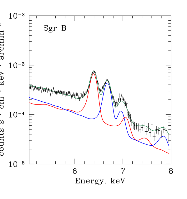
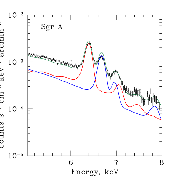
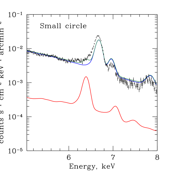
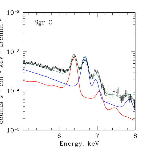
Figure 3: The spectra (black crosses) in the 5-8 keV band extracted from the four circular regions shown in Fig. 2. These spectra are modelled as a linear combination of two spectral templates: $kT=$6 keV optically thin plasma emission (blue) and reflected emission for $\tau_{T}=0.5$ and $\theta=90$^∘(red line, see §2.3). Only the normalizations of both components are free parameters of the model. The green line shows the sum of the two components. In the three regions, where the reflected component is strong, the contributions of both components to the continuum are comparable.

3.2 Maps of the reflected emission

Given the success of the template fitting in selected regions (see, §3.1), we use the same approach to make a map of the reflected component. Since our model is linear, we can easily do the decomposition by calculating in every pixel of the image the scalar products of the observed spectra with the two spectral templates in the 5-8 keV band, and solve for the best-fitting amplitudes. When calculating scalar products, the template spectra have been convolved with the instrument spectral response. The maps of the two components (best-fitting amplitudes for each template) derived from XMM-Newton data are shown in the two lower panels of Fig. 2. The maps have been adaptively smoothed to reach the required level of statistics (number of counts in the 5-8 keV band per smoothing window).

The resulting maps appear qualitatively similar to the 6.4 keV maps derived in (e.g. Soldi et al., 2014; Ponti et al., 2014), confirming that this simple approach can be used to reveal the morphology of the reflected emission and estimate its flux. A more elaborate spectral analysis is done below.

3.3 Difference spectra

Even a more convincing and powerful spectral test on the nature of the “reflected” component is possible for regions where we see significant variability of the diffuse emission. This is illustrated in Fig. 4, where the difference between the spectra labelled as A and B, obtained during two different epochs, are shown. For this exercise, the Chandra data in 2000-2008 and 2009-2015 were used. We extracted the spectra from the red circle in Fig. 4, where variability of the diffuse emission flux was particularly strong. In the difference spectrum, all steady components must be gone and we expect to see a pure reflection component. This procedure effectively simplifies the spectral modeling and therefore can be used to place stronger constraints on the reflected component alone. Indeed, the difference spectrum can be well described by a pure reflection model with $\tau_{T}\sim 0.02$, cosine of the scattering angle $\mu\sim 0$ and an additional hydrogen column density of absorbing gas $N_{H}\sim 1.7~{}10^{23}~{}{\rm cm^{-2}}$. Potentially this approach provides the most robust way to spectrally determine the position of the cloud along the line of sight, since the shape of the spectrum, e.g., the equivalent width of the 6.4 keV line, depends on the scattering angle due to the difference in the angular distributions for scattered and fluorescent photons (see, e.g., Sunyaev & Churazov, 1998; Capelli et al., 2012) avoiding the necessity of modelling complicated background/foreground. However, there are several caveats. One caveat is the abundance of iron (and heavy elements in general), and as a consequence, the expected equivalent width of the line is uncertain. The second is the geometry of the cloud that is important in the case of substantial optical depth of the cloud. The last uncertainty is purely instrumental and applies to the case shown in Fig. 4 - we used both ACIS-I and ACIS-S for this analysis, correcting for the differences in the effective area, but neglecting the difference in energy resolution, which is clearly an oversimplification. This is the reason why we quote above the approximate values of the parameters without uncertainties. However, neither of these caveats is crucial and could be overcome to improve such analysis. If we ignore these complications, e.g., assume that the abundance used in the model is correct, then the minimal $\chi^{2}$ is achieved for $\mu=-0.3$ (scattering angle $\sim$110^∘​) and, at $\sim$90% confidence, $|\mu|<0.4$. This implies that the cloud is located $\sim 8$ pc further away from us than Sgr A^∗. We note that this result agrees well with the position estimate obtained by Churazov et al. (2017) using the completely independent technique, although uncertainties in both approaches are large.

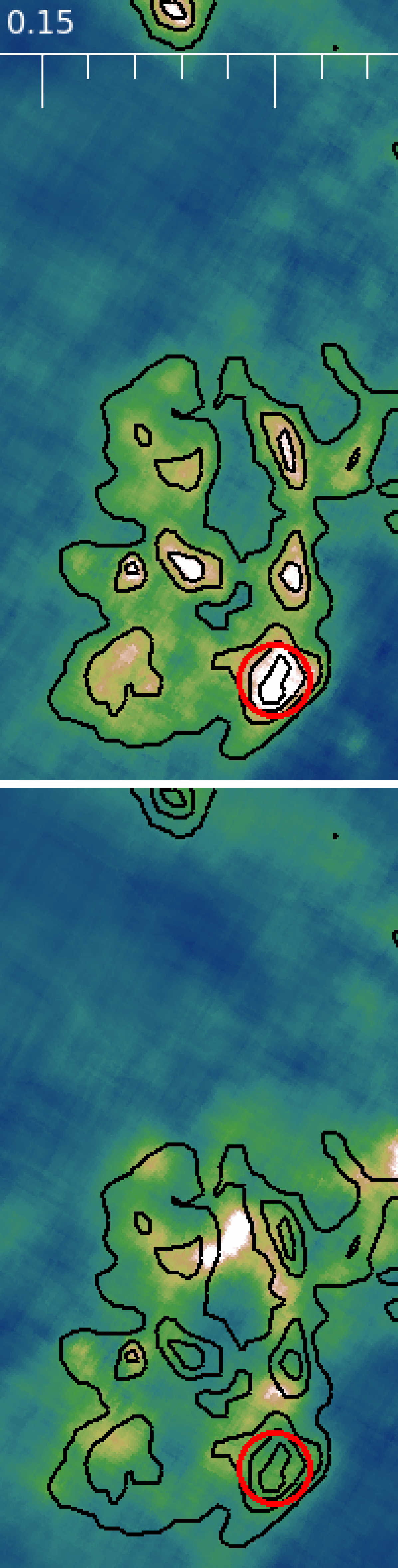
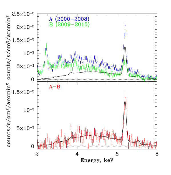
Figure 4: Spectrum of a reflection component “cleaned” for the background contribution. Left: Chandra maps of the scattered emission in Sgr A^∗ region [modified version of the figure from Churazov et al. (2017)]. Images are in Galactic coordinates (see axis, $(l,b)$ in degrees). The top and bottom images show the maps averaged over 2000-2008 and 2009-2015 data, respectively. Contours on both images correspond to the top image to emphasize the difference in the maps. The red circles shows the region used to extract the spectra, A and B for the top and bottom images, respectively. In the 2000-2008 data, the reflected emission from this region was significantly brighter. Top-right: The A and B spectra, extracted from the region shown with red circle, are shown with blue and green colours, respectively. The A spectrum is clearly brighter than the B spectrum. Bottom-right: The difference between A and B spectra (red crosses). The difference spectrum removes the constant diffuse emission leaving the “pure” reflected component. The black line shows the best-fitting model of the reflected spectrum.

4 Single-scattering approximation and time variability

In the previous section we have used detailed Monte Carlo simulations (including multiple scatterings) of an isolated spherical cloud illuminated by a distant steady primary source. We now would like to allow for a more elaborate geometry of the gas distribution and include variability of the primary source.

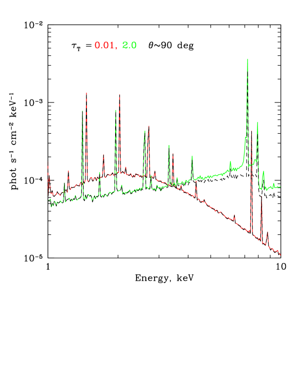
Figure 5: Comparison of a single-scattering approximation with a full Monte Carlo treatment. The red and green curves correspond to the same spectra as shown in the left panel of Fig. 1 for $\tau_{T}=0.01$ (red) and $\tau_{T}=2$ (green) cases. The black dashed lines show the contribution of the single-scattering component to these spectra. Clearly, the single-scattering approximation works well in both limits of small and large optical depths, except for the Compton shoulder of fluorescent lines (on the low-energy side of each line). As in Fig. 1, for clarity the plotted spectra are slightly shifted in energy.

As the first step we note that for neutral gas with solar (or super-solar) abundance of heavy elements, the photoelectric absorption cross section is larger than the scattering cross section at energies below $\sim$10 keV. This means that the role of multiple scatterings is subdominal in this energy range for any value of the optical depth. Indeed, in the limiting case of a small optical depth, the probability of an additional scattering is simply proportional to $\tau_{T}\ll 1$. In the opposite limit of an optical thick medium, the probability of the scattering is set by the ratio of the scattering cross section $\sim\sigma_{T}$ to the total cross section $\sigma\sim\sigma_{T}+\sigma_{ph}(E)$, where $\sigma_{ph}(E)$ is the photoelectric absorption cross section. Since this ratio is small (for energies lower than $\sim$10 keV), the probability of an additional scattering is also small. As a simple illustration we show in Fig. 5 several spectra calculated in §2 (see, Fig. 1, left panel) and the contribution to these spectra from the photons, scattered only once (dashed lines). It is clear that except for the Compton shoulder to the left from the iron fluorescent line, the single-scattering approximation works well over the entire 2-10 keV range. The calculation of the reflected spectra, their variability and polarisation properties is straightforward in the single-scattering approximation. Below we use this approximation to compute maps and variability of the reflected component in the entire GC region.

4.1 Distribution of molecular gas

To simulate the properties of the reflected emission in the GC region, we need a model of the 3D distribution of the gas in this region. Large sets of high-quality sub-mm, IR and molecular data are available for the central 1^∘​ region around the Galactic Center owing to its extensive surveying in recent years (Dahmen et al., 1998; Tsuboi, Handa, & Ukita, 1999; Pierce-Price et al., 2000; Stolovy et al., 2006; Molinari et al., 2011; Jones et al., 2012). Still, these data are capable of providing position-position-velocity (PPV) information at best, so one has to assume some PPV vs. 3D position correspondence in order to fully reconstruct 3D distribution of the dense gas. Several models have been put forward to describe the observed (rather complicated) PPV-distribution of the gas in the region of interest in a concise and physically motivated way, such as the ’twisted ring’-model proposed by Molinari et al. (2011) on base of the Herschel Hi-GAL survey, or the orbital solution by Kruijssen, Dale, & Longmore (2015) [for a thorough comparison of these models with the data provided by various gas tracers see Henshaw et al. (2016)]. Here we adopt the model of Kruijssen, Dale, & Longmore (2015) as a baseline. Although all such models are perhaps too simplistic for comprehensive description of the gas distribution, it is well-suited for our purpose, namely to get characteristic values of the expected reflected component fluxes and polarization degrees over the central 1^∘​ region around the Galactic Center.

In order to estimate the actual gas density along the path described by the orbital solution of Kruijssen, Dale, & Longmore (2015), this solution was used in conjunction with the CS (1-0) data by Tsuboi, Handa, & Ukita (1999). Namely, we extracted the cells from the Tsuboi, Handa, & Ukita (1999) data cube, which falls sufficiently close to the PPV trajectory of Kruijssen, Dale, & Longmore (2015), i.e. that the maximum projected distance of a cell to the trajectory is not more than 2 arcmin and the maximum difference along the velocity axis is 10 km/s. Every cell extracted in this way was treated as a spherical cloud with diameter equal to the cell width in sky projection, whilst its total H₂ mass is calculated according to the standard conversion procedure described in Section 4.2 of (Tsuboi, Handa, & Ukita, 1999) (namely, the fractional abundance of CS molecule is adopted at X(CS)=$1\times 10^{-8}$ level and the excitation temperature $T_{ex}=50$ K). In order to eliminate gridding effects, additional Gaussian scatter of the cloud positions was applied.

On top of this, we separately added the Sgr B2 cloud, since the CS emission as a density tracer becomes increasingly less accurate for that massive molecular clouds as a result of self-attenuation (Tsuboi, Handa, & Ukita, 1999; Sato et al., 2000). Nevertheless, detailed density distribution inside the Sgr B2 cloud can be reconstructed by means of less optically thick tracers along with radiative transfer simulations (Schmiedeke et al., 2016). For the purpose of the current study, however, the finest sub-structures are not very important, since only a small fraction of the total mass ($\sim$1%) is associated with them. Moreover, the reflected signal from them is additionally weakened since they are typically embedded in larger shells of less dense gas (see e.g. a schematic Fig.1 in Schmiedeke et al. 2016). Hence, we implemented only low and moderate density envelopes, and Sgr B2 North, Main and South cores as described in the Table B.3 of Schmiedeke et al. (2016). The total mass of the Sgr B2 complex included in our calculation is $\approx 2.2\times 10^{6}M_{\odot}$, while the total mass of the molecular gas extracted along the trajectory of Kruijssen, Dale, & Longmore (2015) is $\approx 9.2\times 10^{6}M_{\odot}$. We note here that only a fraction ($\sim 30\%$) of the total molecular gas in CMZ ($\sim 2-6\times 10^{7}M_{\odot}$, Dahmen et al. 1998; Tsuboi, Handa, & Ukita 1999; Pierce-Price et al. 2000; Molinari et al. 2011) has been accounted for by this procedure. In the base-line model the Sgr B2 cloud is placed at the same distance as Sgr A^∗. We consider different line-of-sight positions of the clouds in §5.3.

The resulting simulated distribution of the molecular gas is shown in Fig. 6. The left and right panels show the projected column density of the gas onto $l,b$ and $l,z$ planes, respectively, where $l$ and $b$ are the Galactic coordinates and $z$ is the distance along the line of sight. The simulated volume has the size of $300\times 75\times 300$ pc along $l$, $b$ and $z$ coordinates. The large diffuse object in the left side of the plots corresponds to the Sgr B2 complex placed at the same distance as Sgr A^∗.

This model certainly is a gross simplification of the true (unknown) distribution of the gas. For instance, this model is completely devoid from the gas in the innermost region around Sgr A^∗, while there is clear evidence for the dense molecular clouds in this region, such as the circumnuclear disc (Becklin, Gatley, & Werner, 1982; Requena-Torres et al., 2012) and the 50 km s^-1 cloud interacting with the Sgr A East (Coil & Ho, 2000; Ferrière, 2012). Also, it does not include the molecular Sgr A/“Bridge” complex (Fig. 6), which is likely located not further than $\sim 25$ pc from Sgr A^∗ (Churazov et al., 2017). In future, the data on the degree of polarization (§5.3) can differentiate between scenarios that differ in the absolute value of the line-of-sight position $|z|$ of the scattering cloud relative to the illuminating source. For now, the model shown in Fig. 6 is suitable only for qualitative characterization of the long-term evolution of the polarization and flux of the reflected flux.

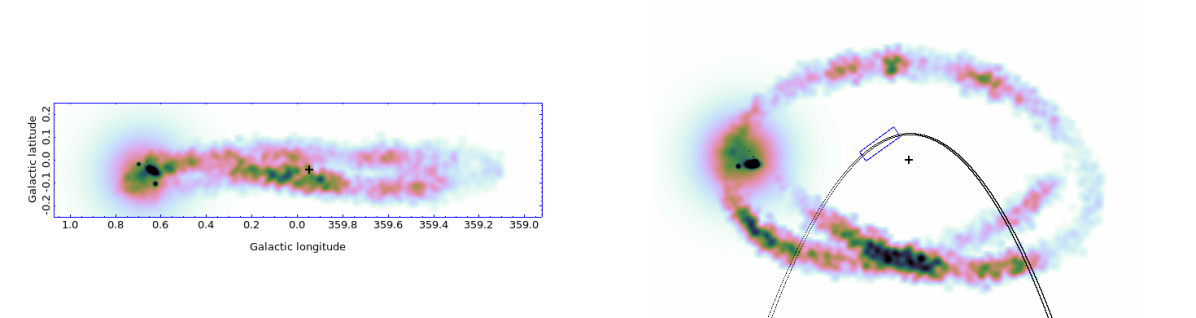
Figure 6: Model of the distribution of the molecular gas in the $300\times 70\times 300$ pc box (see §4.1 for details). Left: Projected gas column density onto $(l,b)$ plane. Right: Projected gas column density onto $(l,z)$ plane (view from the top). The large diffuse object in the left side of the plots corresponds to the Sgr B2 complex. In the base-line model the Sgr B2 cloud is placed at the same distance as Sgr A^∗. We consider different line-of-sight positions of the clouds in §5.3. The position of Sgr A^∗ is marked with the black cross. Thin black lines shows illiminated region for a model of a short outburts $\sim$110 yr ago (see Churazov et al., 2017). The rwo lines correspond to the beginning and the end of a 5 yr long flare. The blue box shows the region where molecular gas should be located in the model of Churazov et al. (2017) to provide bright X-ray emission from the so-called ”Bridge” region. There is a clear tension between the models, suggesting that either the gas distribution model is incomplete (see §4.1) or the X-ray emission from the ”Bridge” is due to much more recent ($\sim$20 yr ago) or much older ($\sim$400 yr) flare that illuminates the front or the back parts of gas distribution shown in the figure. The degree of polarization of the reflected emission from the ”Bridge” is expected to be much smaller in the ’recent’ and ’old’ flare scenarios (see §5.3), compared to the flare that happened $\sim$ 110 yr ago.

4.2 Illuminating source

We assume that the primary source is located at the position of Sgr A^∗, namely, $(l_{0},b_{0},z_{0})=(-8,-7,0)$ pc. The light curve of the source is modelled as a single outburst, that starts at time $t_{1}$ and ends at $t_{2}$, so that the duration of the outburst is $t_{b}=t_{2}-t_{1}$. For our illustrative run we have chosen $t_{b}=50~{}{\rm yr}$, $t_{1}=0$ and $t_{2}=50$, i.e. the beginning of simulations at $t=0$ corresponds to the onset of the outburst. Motivated by the estimates of the flux from Sgr A^∗ required to explain the fluorescent emission from the Sgr B2 clouds (see, e.g., Sunyaev & Churazov, 1998), we set a fiducial 2-10 keV luminosity of the source during the outburst to $L_{X}=10^{39}~{}{\rm erg~{}s^{-1}}$ with a power law spectrum with index $\Gamma=2$ (Revnivtsev et al., 2004; Terrier et al., 2010; Mori et al., 2015; Zhang et al., 2015). As in §2 the emission of the primary source is assumed to be unpolarized.

4.3 Absorption, Scattering, Polarization and Fluorescent Lines

In the single scattering approximation approach the calculation of the observed flux is straightforward. For a given cell $(l,b,z)$ of the 3D box, the time delay $\Delta t$ from the primary source, Sgr A^∗, to the scattering cell and then to observer is

$$\Delta t=\left(\sqrt{(l-l_{0})^{2}+(b-b_{0})^{2}+(z-z_{0})^{2}}-(z-z_{0})\right)/c$$ (2)

where $(l_{0},b_{0},z_{0})$ pc are the coordinates of the primary source and $c$ is the speed of light. Thus, the observer time $t$ translates into the primary source time as $t_{s}=t-\Delta t$. If the value of $t_{s}$ falls in between $t_{1}$ and $t_{2}$, i.e., the time when the source is in outburst, the flux $F(E)$ illuminating this cell is calculated as

$$F(E)=\frac{I(E)}{4\pi D^{2}}e^{-\tau_{1}(E)},{\rm~{}where}$$ (3)

$$\tau_{1}(E)=(\sigma_{T}+\sigma_{ph}(E))\int n(s)ds.$$ (4)

In the above expression, $n$ is the gas density, $s$ is a coordinate along the line connecting the primary source and the cell, $\tau_{1}(E)$ is the optical depth along this line and $D$ is the distance from the primary source to the cell. Here $I(E)$ is the flux of the primary source, such that $L_{X}=\int_{2}^{10}I(E)EdE$.

When calculating the scattered flux, including polarization, we use Thomson differential cross section and store the polarized and the total flux for each cell. Since we are using single-scattering approximation, the orientation of the polarization direction is fully defined by the relative positions of the primary source, the observer and the scattering cell. In projection to the $l,b$ plane the polarization direction is perpendicular to the line connecting $(l,b)$ position of the cell and the primary source $(l_{0},b_{0})$. The procedure of calculating the scattered flux is repeated for all energies.

The fluorescent lines of all astrophysically abundant elements are included in the calculations and added to the corresponding bins of the scattered spectrum. The fluorescent flux is emitted isotropically and is not polarized.

The final step is the projection of the scattered flux onto $(l,b)$ plane, taking into account additional attenuation factor $e^{-\tau_{2}(E)}$ due to the scattering and absorption along the line connecting the cell and the observer. Any additional attenuation outside of the simulated box is ignored in the calculations, but can be easily added as a multiplicative factor to the calculated spectrum.

5 Time evolution, spectra and polarization based on the 3D model

5.1 Time evolution

We illustrate the expected time evolution of the reflected emission produced by a 50 yr long outburst in Fig. 7 (left panel) . Initially, the outburst illuminates the “near” side of the molecular gas distribution, which corresponds to the crossing streams in front of Sgr A^∗ (see the right panel of Fig. 6). The illuminated region quickly expands ($\sim$50 yr) since for the gas lying in front of the primary source, the apparent velocity of motion is very high (see, e.g., Sunyaev & Churazov, 1998). The flare then moves to the sides (200 yr), then it illuminates the more distant side of the trajectory, lying behind Sgr A^∗ (400 yr) and finally it fades away (500 yr).

For comparison, Fig. 7 (right panel) shows the evolution for a shorter outburst with $t_{b}=5$ yr. For this run the luminosity was increased by a factor of 10, i.e. $L_{X}=10^{40}~{}{\rm erg~{}s^{-1}}$. Thus, the total amount of energy released by the outburst $L_{X}t_{b}$ was the same as for the longer outburst. In general, both scenarios share many morphological features, although there are differences caused by the different values of $t_{b}$. In particular, during the early phase the bright spots are more compact (see, e.g., a snapshot at 50 yr after the onset of the outburst). Also, for compact clouds, which have their entire volume illuminated by a flare, the surface brightness is sensitive to the luminosity of the outburst rather than to the fluence. As the result, such clouds appear brighter in our $t_{b}=5$ yr scenario. In contrast, for larger clouds the surface brightness is more sensitive to the fluence, and they appear equally bright in both scenarios.

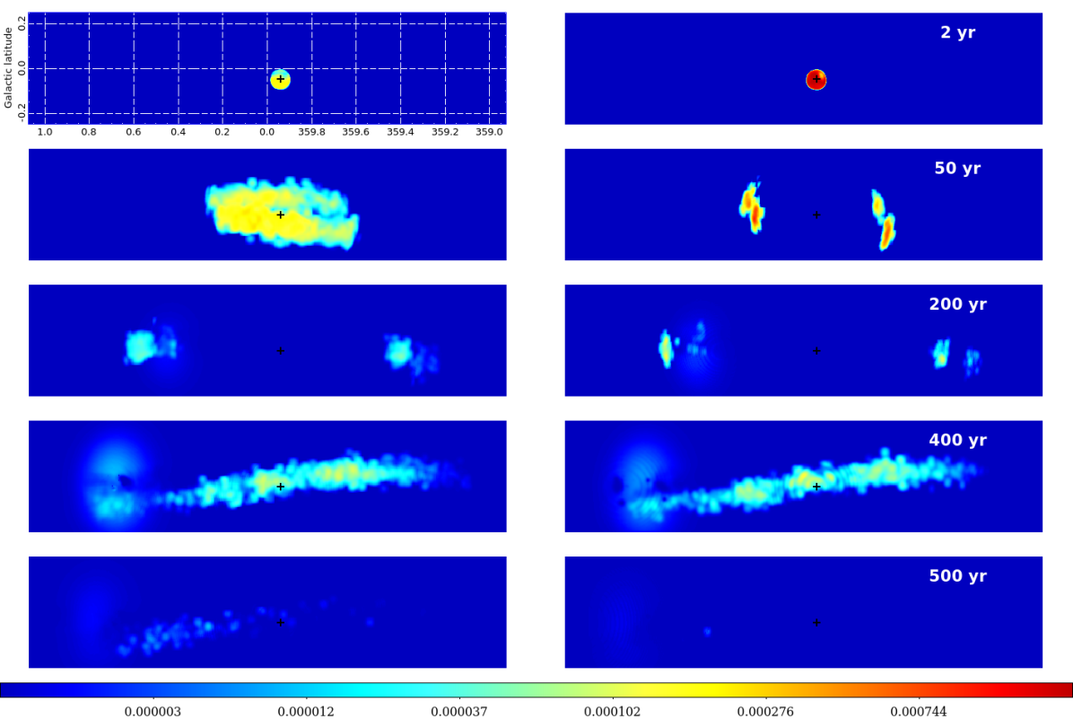
Figure 7: Maps of the reflected component flux as a function of time for a single outburst of Sgr A^∗ (position of Sgr A^∗ is marked with the cross). The left panel corresponds to a 50 yr long outburst, while the right panel shows the case of a shorter 5 yr long outburst. The luminosity of the central source is 10 times larger for the 5 yr outburst, to provide the same fluence as for the longer outburst. The maps shown for moments $t=$2, 50, 200, 400, 500 yr (from top to bottom; indicated in the right panel) since the onset of the outburst. The gas density distribution is described in §4.1 and shown in Fig. 6. As time progresses, the reflected signal first “spreads” to the sides from the primary source (2, 50, 200 yr frames) and then lights-up (frame 400 yr) the more distant part of the molecular arm (see Fig. 6) and the Sgr B2 cloud. 500 yr after the outburst the photons leave the simulated region and the reflected component fades away. Dark lanes across Sgr B2 cloud, seen in the 400 yr frame, are caused by the scattering/absorption along the path of the photons going from the primary source to the scattering cell and then to the observer. Naturally, any complicated time evolution of the primary source flux would lead to a distribution of the reflected emission that can be described as a linear combination of images, corresponding to short flares happening at different times. For instance, a sum of all five images in the right column would describe the expected outcome of five equal flares that happened 2, 50, 200, 400 and 500 years ago.

A similar exercise of modelling the long-term evolution of the reflected emission was done by Clavel et al. (2014), using the twisted ring model of Molinari et al. (2011). Qualitatively the predictions are similar, implying that different patches within 100 pc from the GC should brighten or fade away over hundreds of years. In Churazov et al. (2017) we argued that it is possible to determine the location of molecular complexes along the line of sight by comparing the properties of spatial and time variations of the signal. The estimates based on this approach suggest that the Fe K$\alpha$ bright part of the Sgr A complex (see Fig. 2) is located $\sim$10 pc further away from Sgr A^∗. This is not consistent with the 3D gas distributions in the models of Molinari et al. (2011) or Kruijssen, Dale, & Longmore (2015). This is not surprizing, given that significant fraction of the gas is not accounted for by the model adopted here (see §4.1). Therefore, more work is needed to unambiguously position molecular clouds in 3D. However, it is clear that once few clouds are accurately positioned and the light curve properties of the primary source are determined (presumably via observations of several very localized clumps) the true power of the X-ray tomography of the molecular gas can be employed. One of the possible way to determine the position of a cloud along the line of sight is to measure the degree of polarization, discussed in the next subsection.

5.2 Polarization maps

The calculation of polarization in the single-scattering approximation is straightforward (see also Churazov, Sunyaev, & Sazonov, 2002, for the discussion of polarized flux after muliple scatterings), since the direction and the degree of polarization depend only on the scattering angle. Of course in real observations an additional, presumably unpolarized, background/foreground emission should be present. One can use existing XMM-Newton images (see Fig. 2 and Ponti et al. 2015) to approximately account for the contribution of this emission by assuming that the observed emission is unpolarized and adding this unpolarized signal to the simulated emission of the scattered component. In Fig. 8 we show the expected polarization of the continuum emission in the 4-8 keV band obtained by combining simulated and observed images.

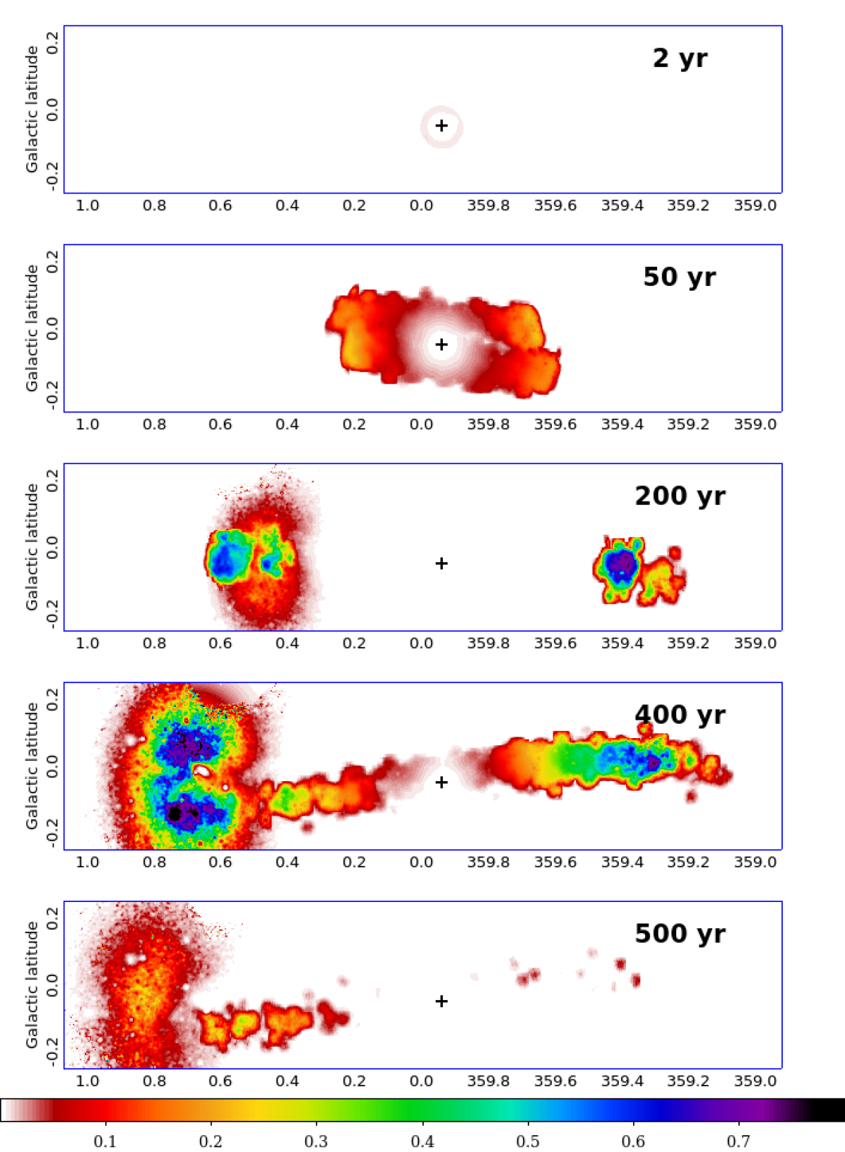
Figure 8: Expected degree of polarization for the continuum in the 4-8 keV band (excluding fluorescent lines), obtained by combining the observed X-ray 4-8 keV image (see top panel in Fig. 2) with the simulated maps (see Fig. 7). The colorbar at the bottom of the plot shows the degree of polarization. The 50 yr long outburst model is used to simulate the reflected emission. All five panels correspond to the same moments (2, 50, 200, 400, 500 yr) as in Fig. 7. For the central regions the degree of polarization is always low, since the scattering angle is either small or close to 180^∘(given the 3D geometry shown in Fig. 6). The largest degree of polarization is expected for the Sgr B2 cloud, since in these simulations it is located at the same distance as Sgr A^∗.

The five panels shown correspond to the same moments (2, 50, 200, 400, 500 yr) as in Fig. 7. For the central regions the degree of polarization is always low, since there the scattering angle is either small or close to 180^∘​ (given the 3D geometry shown in Fig. 6). The largest degree of polarization is expected for the Sgr B2 cloud, since in these simulations it is located at the same distance as Sgr A^∗. Note also, that the degree of polarization shown in Fig. 8 depends both on the intrinsic degree of polarization $p_{int}$, set by the scattering angle, and the relation between the intensity of reflected $I_{R}$ emission relative to the unpolarized background $I_{B}$, i.e. $p=p_{int}/(1+I_{B}/I_{R})$. The reflected intensity depends on the luminosity of the illuminating source and the duration of the outburst, while the intrinsic polarization depends only on the geometry of the problem.

5.3 Spectra and polarization

A more accurate estimate of the reflected emission and the degree of polarization can be easily obtained in the single-scattering approximation by calculating the expected spectra. For this purpose, we used a 15 pc (radius) circle centered at the Sgr B2 position and calculated the total spectrum coming from this region. We then repeated the same exercise varying the position of the centre of the Sgr B2 cloud along the line of sight ($z=-100,0,100$ pc). The resulting spectra are shown in the right panel of Fig. 9. The left panel of the figure shows the snapshots corresponding to the moments when the cloud is illuminated by the outburst.

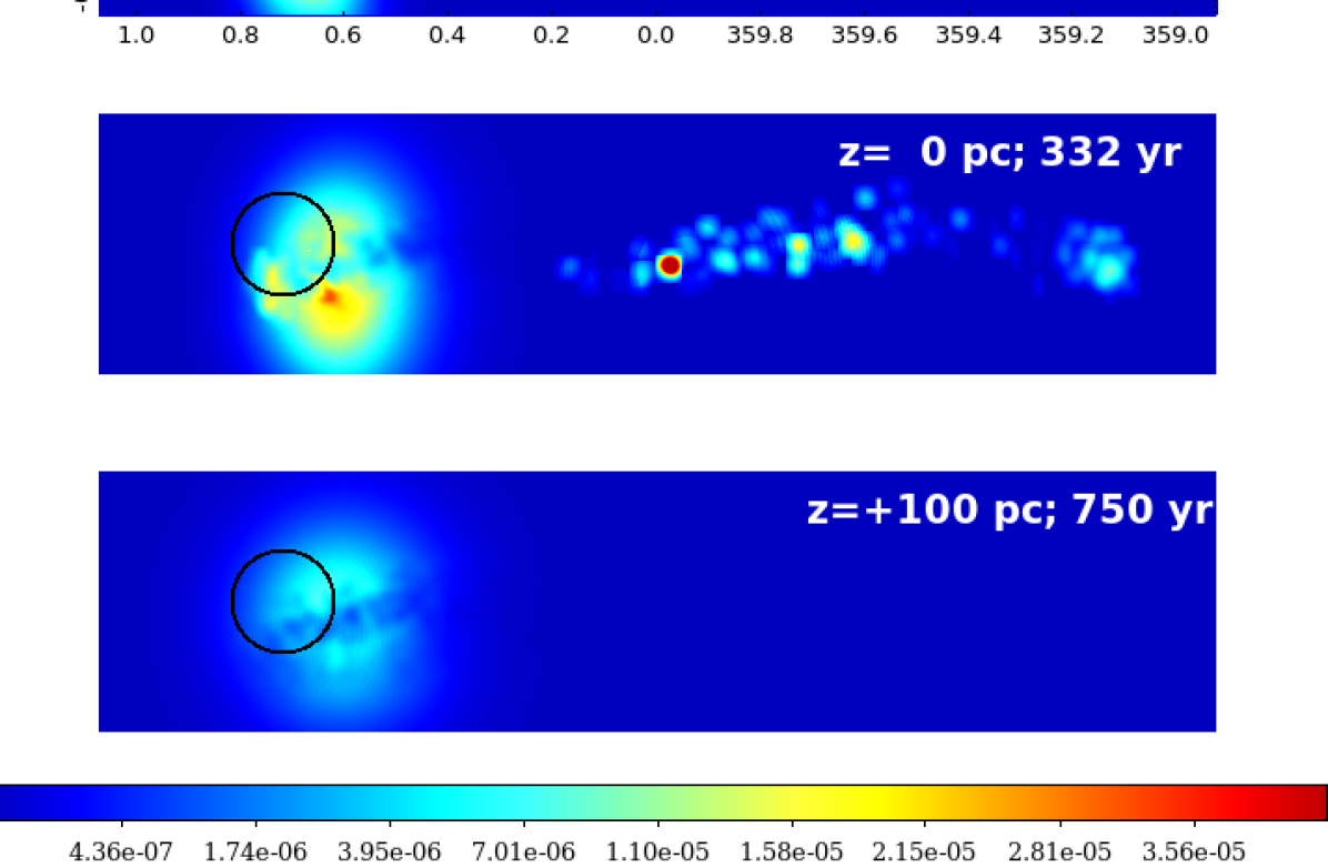
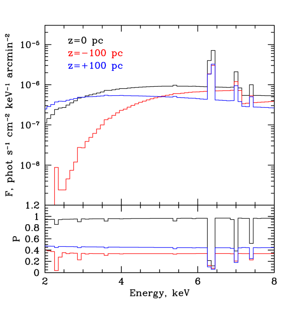
Figure 9: Expected spectra for different positions of Sgr B2 along the line of sight. Left: Maps of the scattered emission in the 4-8 keV band. The clouds is placed at -100, 0, +100 pc, relative to Sgr A* (from top to bottom). The time of the observation is 170, 332, 750 yr after the outburst for these three panels. Top-right: The spectra of the reflected component, corresponding to three panels on the left are shown by the red (-100 pc), black (0 pc) and and blue (+100 pc) lines. Bottom-right: The degree of polarization for the scattered component. As expected, the degree of polarization is close to 100% for the case when the cloud is at the same distance as the primary source (the black line), but drops significantly if the centre of the clouds is shifted along the line of sight by $\pm 100$ pc (red and blue lines).

As expected the degree of polarization changes with the scattering angle as $\displaystyle p=(1-\mu^{2})/(1+\mu^{2})$, i.e. it is close to 100% for the case when the cloud is at the same distance as the primary source (the black line), i.e., $p\sim 1$. Shifting the cloud by $\pm 100$ pc, implies $|\mu|\sim 0.7$ and $p\sim 35$%. The actual values of polarization are slightly larger (blue and red lines) than this value because the angular size of the cloud (as seen from the Sgr A^∗ position) is large and for the selected snapshots the effective scattering angle is slightly larger. As expected (see, e.g., Churazov, Sunyaev, & Sazonov, 2002), the degree of polarization drops at the energies of prominent fluorescent lines. Note, that the degree of polarization in Fig. 9 is computed for pure reflected component. As we have shown in §3 the contribution of the unpolarized continuum in the regions with prominent reflected components is $\sim$50%. Therefore, we expect the observed polarization to be factor of $\sim$2 smaller.

6 Prospects for XIPE

6.1 Feasibility

The aim of the polarization measurements is three-fold:

• Establish a non-zero polarized signal of the continuum emission as a proof that it is due to scattered emission;

• Find the polarization angle to identify the location of the primary source;

• Measure the degree of polarization to estimate the line-of-sight location of the scatterer relative to the primary source.

In this section we evaluate the ability of the XIPEmission (Soffitta et al., 2013) to detect polarized reflected emission from the GC molecular clouds. Below we use the effective area and the modulation factor from Soffitta et al. (2013). A similar question has already been addressed in Marin et al. (2015) based on the assumed positions of several clouds. In our simulations the uncertainties in the choice of the 3D gas distribution and the parameters of the outburst are considerable. Moreover, we believe that some of the regions that are bright in the reflected component, are not adequately described by this model (see Churazov et al., 2017). We therefore consider simulations as a guideline, but use actual XMM-Newton observations to estimate the fluxes.

From the observed and simulated spectra (see Figs. 1, 2, 9) it is clear that at low energies the photoelectric absorption can suppress the reflected component if a cloud is illuminated from the back. At the same time, above $\sim$6 keV the spectrum is dominated by the 6.4 keV from neutral iron and 6.7-6.9 keV lines from the hot plasma. Since we expect the emission in these lines to be unpolarized, it does not make sense to use the energy range 6-7.5 keV when searching for polarized emission. Thus, we have selected an energy band from 3 to 6 keV for the feasibility study. The problem of evaluating the degree of polarization and the polarization angle was discussed recently by Weisskopf, Elsner, & O’Dell (2010); Strohmayer & Kallman (2013); Montgomery & Swank (2015). Here we adopt the simplest approach possible. To estimate the expected S/N, we have extracted spectra from three $4^{\prime}$ (radius) circles from the Sgr B2, the “Bridge” and Sgr C regions. For this purpose all publicly available XMM-Newton (MOS) data were used. Only the data in the 3-6 keV band, where continuum emission dominates, were used for the sensitivity estimates. As mentioned in §3 it is reasonable to assume that in these regions about half of the signal is due to the reflected component, while another half is due to (unpolarized) background/foreground emission.

We assume that for a source with a polarization angle $\phi_{0}$ the signal recorded by a polarization-sensitive detector is described by the following expression

$$D(\theta)=[B+S]+[Spm]\cos 2\left(\theta-\phi_{0}\right)+\eta,$$ (5)

where $\theta$ is the phase, $B$ is the intensity of a steady (unpolarized) background, $S$ is the sources flux, $p$ degree of polarization of the source flux, $m$ is the known modulation factor in this energy band and $\eta$ is the noise that we assume, for simplicity, to be Gaussian and the same for all phases. We further assume that the background is known and set $B=0$.

This signal can be approximated with a model

$$M_{1}(\theta)=C_{1}+C_{2}\cos 2\left(\theta-\phi\right),$$ (6)

where $C_{1}$, $C_{2}$ and $\phi$ are the parameters of the model. Even more convenient is the parametrization

$$M_{2}(\theta)=A_{1}+A_{2}\cos 2(\theta)+A_{3}\sin 2(\theta),$$ (7)

where $A_{1}$, $A_{2}$ and $A_{3}$ are free parameters. The best-fitting values can be determined via simple $\chi^{2}$ minimization,

$$\chi^{2}=\Sigma_{\theta}\left(\frac{M(\theta)-D(\theta)}{\sigma}\right)^{2}\rightarrow{\rm min},$$ (8)

where $\sigma^{2}=Var(\eta)$ is the variance of the noise $\eta$. The advantage of the second model is that the explicit expressions of the best-fitting parameters $A_{1}$, $A_{2}$ and $A_{3}$ can be immediately written as

$$\sum_{\theta}D(\theta)f(\theta)/\sum_{\theta}f^{2}(\theta),$$ (9)

where $f(\theta)=1$, $\cos(2\theta$) and $\sin(2\theta)$ for $A_{1}$, $A_{2}$ and $A_{3}$, respectively. The values of $A_{1}$, $A_{2}$ and $A_{3}$ have Gaussian distributions with standard deviations $\sigma_{A_{1}}=\sigma/\sqrt{n_{\theta}}$, $\sigma_{A_{2}}=\sigma_{A_{3}}=\sqrt{2}~{}\sigma_{A_{1}}$. Note, that functions $f$ for different $A$’s are mutually orthogonal, i.e., resulting contributions of the noise to $A_{1}$, $A_{2}$ and $A_{3}$ are uncorrelated. The number of bins $n_{\theta}$ over $\theta$ should be sufficiently large to properly sample the model. Even if the actual number of counts per bin is small, but the total number of counts is $\gg 1$, the $\chi^{2}$ minimization can still be used (Churazov et al., 1996) to get an unbiased estimate of the best-fitting parameters and correct confidence regions.

6.2 Known polarization angle

If the polarization angle $\phi_{0}$ is known (e.g., when the location of a primary source is known) the minimization for the model given by equation (6) reduces to a linear problem and explicit expression for the coefficients $C_{1}$ and $C_{2}$ can be easily written. In the frame of this model the expected significance of the polarized signal detection $S_{p}$ is simply

$$S_{p}=\frac{pm}{\sqrt{2}}\frac{S\sqrt{n_{\theta}}}{\sigma}=\frac{pm}{\sqrt{2}}S_{C_{1}}$$ (10)

where $S_{C_{1}}\equiv S_{A_{1}}=S\sqrt{n_{\theta}}/\sigma$ is the expected signal-to-noise ratio for $C_{1}\equiv A_{1}$ value, i.e., the significance of the total source flux detection. This expression can be easily generalized for an arbitrary spectral shape and energy dependent modulation factor and polarization.

6.3 Null hypothesis of zero polarization

We can now relax the assumption that the angle is known and use the model given by equation (7) to obtain best-fitting values of $A_{1}$, $A_{2}$ and $A_{3}$. Consider first a case when true polarization of the source is zero, i.e., $p=0$. The probability $P$ of finding a value of $x=\sqrt{A_{2}^{2}+A_{3}^{2}}$ larger than a certain threshold $t$ is, obviously,

$$P(x>t)=e^{-\frac{t^{2}}{4\sigma^{2}_{A_{1}}}}.$$ (11)

The above expression can be used to determine the significance of the polarization detection in observations. For the feasibility studies the minimum detectable polarization $p_{min}$, given total source flux detection significance $S_{A_{1}}$ and the probability of false detection $P$ (e.g., $P=10^{-3}$), is simply

$$p_{min}=\frac{1}{m}\frac{2}{S_{A_{1}}}\sqrt{-\log P}.$$ (12)

6.4 Confidence regions

We now outline the simplest procedure of estimating the confidence regions from the observed data. Given the best-fitting values of $A_{1}$, $A_{2}$ and $A_{3}$ the angle $\phi$ and polarization $p$ can be evaluated as

$$\phi=\frac{1}{2}\arctan\left(\frac{A_{3}}{A_{2}}\right)$$ (13)

$$p=\frac{\sqrt{A_{2}^{2}+A_{3}^{2}}}{A_{1}m}=\frac{x}{A_{1}m},$$ (14)

where as before $x=\sqrt{A_{2}^{2}+A_{3}^{2}}$. The value of $\phi$ does not depend explicitly on $A_{1}$, while the expression for $p$ includes $A_{1}$ as a normalization factor. For simplicity, we consider below the confidence regions for the parameters $\phi$ and $x$ that depend only on the values of $A_{2}$ and $A_{3}$.

6.4.1 Confidence region for a pair $(\phi,x)$.

The easiest case is a confidence region for the pair of parameters $(\phi,x)$. Consider a difference in the values of $\chi^{2}$ (equation 8) for a model with a given set of parameters and for the model with best-fitting parameters ($\chi^{2}_{bf}$):

$$\Delta\chi^{2}=\chi^{2}-\chi^{2}_{bf}.$$ (15)

Since the distribution of $A_{2}$ and $A_{3}$ around true values has a bivariate Gaussian distribution, the confidence region in the $(A_{2},A_{3})$ space can be calculated as the 2D region where $\Delta\chi^{2}$ is less or equal to a threshold value $\Delta_{2}$, such that the probability of $\chi^{2}_{2}<\Delta_{2}$ is equal to $P$. Here $\chi^{2}_{2}$ is a $\chi^{2}$ distribution with two degrees of freedom, i.e., for $P=0.9$, $\Delta_{2}=4.61$. The corresponding region in the $(\phi,x)$ will obviously enclose true values of $\phi$ and $x$ each time when a pair of true values $(A_{2},A_{3})_{true}$ is enclosed.

6.4.2 Confidence region for $\phi$ as a single parameter of interest.

We are often interested in the confidence regions separately for $\phi$ and $x$. For $\phi$ (as a single parameter of interest) the confidence region can be evaluated by finding the minimum of the $\chi^{2}$ for each value of $\phi$ (minimizing over $C_{1}$ and $C_{2}$ in equation 6) and selecting the range of $\phi$ such that $\Delta\chi^{2}$ is less or equal to a threshold value $\Delta_{1}$, such that the probability of $\chi^{2}_{1}<\Delta_{1}$ is equal to $P$, where $\chi^{2}_{1}$ is a $\chi^{2}$ distribution with one degree of freedom; i.e., for $P=0.9$, $\Delta_{1}=2.71$. For feasibility studies, when the polarization signal has high significance, i.e. $S_{p}\gg 1$, one can derive a simple estimate of the expected error in $\phi$:

$$\phi_{err}=\frac{1}{2}\arcsin\left(\frac{\sqrt{\Delta_{1}}}{S_{p}}\right)\approx 28.65\left(\frac{\sqrt{\Delta_{1}}}{S_{p}}\right)~{}~{}{[\rm deg]}.$$ (16)

6.4.3 Confidence region for $x$ (and $p$) as a single parameter of interest.

For the value of $x$ (as a single parameter of interest) the recipe of using $\Delta\chi^{2}<\Delta_{1}$ is not exact. This is clear, for instance, in case if true polarization is zero or very small, i.e., $S_{p}\ll 1$. In this limit the model with the true value of polarization is obviously insensitive to the value of $\phi$. In this case the value of $\Delta\chi^{2}$ with respect to the best-fitting model (see equation 7) has a $\chi^{2}$ distribution with two degrees of freedom. However, when the significance of the polarization increases, the accuracy of the confidence evaluation based on $\Delta_{1}$ increases. For $S_{p}\gtrsim 1$ one can already safely use this approach. In real observations the value of $S_{p}$ is not known, but one can use in lieu the significance of non-zero detection of polarized signal.

As the last step (see equation 14), the value of $x$ has to be converted to polarization $p=x/(mA_{1})$. One can expect that in majority of real objects, the total source flux $A_{1}$ will be determined with much higher accuracy than the polarized component $x$. In this case the confidence regions can simply be extended based on the relative uncertainty in $A_{1}$. For most cases this should be an acceptable solution.

6.5 Predictions for XIPE

For the three selected regions we know the flux level of the scattered and background component from the XMM-Newton data and have a reasonable approximation of the spectrum shape in the 3-6 keV band (see Fig. 3). Moreover, the angle $\phi$ is also known, assuming that Sgr A* is the primary source of X-ray radiation. We also know the effective area and the modulation factor of the instrument. What is unknown is the degree of polarization $p$ of the scattered component. The value of $p$ depends solely on the shift $z$ along the line of sight of the scattering site relative to the primary source. One natural assumption would be that $\displaystyle|z|\sim\sqrt{(l-l_{0})^{2}+(b-b_{0})^{2}}$, i.e., the shift along the line of sight is of the same order as the projected distance from the primary source (see, e.g. Churazov et al., 2017). This estimate suggests that $0.35\lesssim p\lesssim 1$ (see §5.3). On the other hand, the 3D model of the gas distribution adopted in §4.1 suggests that in the gas seen in projection close to Sgr A^∗ is located either in front or behind the source with $\displaystyle|z|$ much larger than the projected distance. This would imply much lower degree of polarization. In Table 1 we quote our estimates of the polarization component S/N ratio (see equation 10) assuming $p=0.5$ in the scattered component in all three region (the net polarization with account for unpolarized background will, of course, be factor $\sim 2$ lower). This estimate assumes that the $\phi$ is known. Clearly the polarization can be easily detected even if the intrinsic polarization is 5-10 times lower, corresponding to a scattering angle of $\sim$20 (or 180-20=160) degrees. This scattering angle corresponds to the shift along the line of sight $\sim$3 times larger than the projected distance. This means that it is likely that polarization will be significantly detected for any plausible distribution of scattering clouds and will provide reliable determination of their line of sight positions.

Table 1: Estimated detection significance of polarization from three selected regions within 100 pc from GC with XIPEfor 1 Msec exposure. Flux is the total observed flux by XMM-Newton , i.e., $S+B$ as in equation 5. It is assumed that the contributions of $S$ and $B$ are equal (see §3.1); $p=0.5$ is set for the scattered component $S$.

Region	Flux, 3-6 keV	Detection significance, $S_{p}$	Error on angle, $\phi_{err}$
	${\rm erg~{}s~{}cm^{-2}}$	(for $p=0.5$)	deg  (for $p=0.5$)
Sgr B2	$2\times 10^{-12}$	$\sim$20	$\sim 1.4$
Sgr A /“Bridge”	$1\times 10^{-11}$	$\sim$50	$\sim 0.6$
Sgr C	$2\times 10^{-12}$	$\sim$20	$\sim 1.4$

The above results broadly agree with the previous estimates (Marin et al., 2015) for XIPE, although there are interesting differences. In our case we used the observed X-ray spectra (rather than simulated) for the feasibility study and we used a simple decomposition of the spectra into reflected component and unpolarized one. This makes the predictions insensitive to the modelling in the part related to the intensity of the reflected emission. The main remaining uncertainty is the cloud positions along the line of sight that sets the polarization. Based on our previous study (Churazov et al., 2017) of the variability of the the Sgr A/“Bridge” complex, we believe that this gas is not strongly shifted along the line of sight with respect to the Sgr A*. This therefore predicts high degree of polarization of its reflected emission and makes Sgr A/“Bridge” complex a promising (and, perhaps, even the most promising, given its brightness) target for XIPE.

Given that the majority of the X-ray emitting clouds in the GC region are variable on time scales of few years - decades (see, e.g., Inui et al., 2009; Ponti et al., 2010; Clavel et al., 2013; Mori et al., 2015) it is not possible to make firm predictions on the expected fluxes for future missions more than 1-2 years ahead. Historic observations and our simulations show that it is possible that another set of regions will be bright then. Unless we are particularly unlucky, the flux level of those bright regions will be similar to the flux levels we saw in the past 20-30 years. It therefore makes sense to select targets during the active phase of the mission (or $\sim$1-2 years before).

7 Discussion

7.1 Is Sgr A* the primary source?

In a addition to Sgr A*, the molecular clouds in the Galactic Center region can be illuminated by stellar mass X-ray sources, namely X-ray binaries or flaring magnetars, located in the same region (see, e.g., relevant discussions in Ponti et al., 2013; Rea et al., 2013; Clavel et al., 2013).

Clearly, any powerful source (with luminosity exceeding $10^{39}~{}{\rm erg\,s^{-1}}$) located in the close vicinity of the Galactic Center could mimic Sgr A* flare in terms of the polarization pattern or the long-term variability of the reflected emission. A short-term variability and spectral shape information can be used to distinguish between i) hard and very short ($\lesssim 1$ s) giant magnetar flare (e.g. Hurley et al., 2005), ii) an outburst of a (currently dim) ultraluminous X-ray source ($L_{X}\sim 10^{40}$ erg s^-1) with the spectrum typically characterized by a cut-off like curvature at $\sim 5$ keV (e.g. Walton et al. (2014)), although the detection of the X-ray reflection signal by INTEGRAL (Revnivtsev et al., 2004) and Nustar (Zhang et al., 2015) in the 10-100 keV range argues against the strong cutoff in the spectrum iii) or a longer duration ($\sim 10$ yr) and smaller luminosity ($L_{X}\sim 10^{39}$ erg s^-1) active state of a more secular X-ray binary (e.g. similar to GRS 1915+105).

On the contrary, a bright source shifted from the projected position of Sgr A* would produce different polarization and long-term variability patterns, which can be used to falsify the hypothesis that Sgr A* is the primary source. The variability test works best if the molecular gas distribution is known. On the other hand, the orientation of the polarization plane is least sensitive to the details of the model, except for the mutual projected positions of the source and the cloud. The strongest constraints would come from those clouds (bright in reflected emission) that subtend the largest angle in the $(l,b)$ plane from the Sgr A* position. This strengthens the case of a spatially resolved polarization measurements of the Sgr A/”Bridge” region, which is located close to Sgr A* and subtends almost 70^∘(as seen from Sgr A*).

A more complicated situation arises when multiple illuminating sources are present and/or intrinsic beaming and corresponding variability of the illuminating radiation. The predictions of the resulting reflected signal are discussed, e.g., in Molaro, Khatri, & Sunyaev (2014) and Khabibullin & Sazonov (2016).

7.2 Sgr A* variability

As we have shown in §5, for the adopted gas distribution model, the reflected emission is visible for $\sim 500$ yr after a flare of the illuminating source. Hence, observing reflection signal at different positions across this region in principle allows one to reconstruct the Sgr A* activity over past $\sim 500$ yr. Currently, the observations suggest, that $\sim 100$ yr ago, Sgr A* had an X-ray luminosity in excess of $10^{39}~{}{\rm erg~{}s^{-1}}$ for a period of few years (e.g., Revnivtsev et al., 2004; Terrier et al., 2010; Churazov et al., 2017), which is $10^{6}$ times brighter than the characteristic Sgr A*’s quiescent X-ray luminosity (e.g., Baganoff et al., 2003; Wang et al., 2013). A number of scenarios have been proposed to explain such behavior, including accretion of a stellar material captured from the winds of nearby stars (Cuadra, Nayakshin, & Martins, 2008) or supplied by their tidal interaction (Sazonov, Sunyaev, & Revnivtsev, 2012); complete tidal disruption of a planet (Zubovas, Nayakshin, & Markoff, 2012); partial tidal disruption of a star (Guillochon et al., 2014) or the corresponding X-ray afterglow emission originated from the deceleration of the launched jet by the circumnuclear medium (Yu et al., 2011). These scenarios predict different long-term activity patterns, which can potentially be inferred from observations of the reflected signal. Basically, three distinct patterns might be considered: i) one short flare over the last $\lesssim 500$ yr, which is associated with a relatively rare event (and lucky observer), ii) the same but with the longer flare duration of $\sim 50-100$ yr, iii) a series of short flares separated by few $100$ yr, which can be a manifestation of the secular flaring activity of Sgr A* hypothesized from extrapolation of the observed K-band flux distribution measured over last $\sim 10$ yrs (Witzel et al., 2012) to rare high-flux events.

Along the same lines, one can extrapolate the distribution of X-ray flares (Neilsen et al., 2013; Ponti et al., 2015) from few Msec time scales to $\sim$500 yr. To this end we adopted a pure power law distribution of X-ray fluences $F$ for Sgr A^∗ flares:

$$\frac{dN}{dFdt}\sim 10^{-42}\left(\frac{F}{8\times 10^{36}~{}{\rm erg}}\right)^{-1.5}~{}{\rm flares\,erg^{-1}\,s^{-1}},$$ (17)

that characterizes the number of flares $N$ per unit time per unit interval of fluences In our previous work (Churazov et al., 2017) we estimated the fluence, required to power the emission from the clouds in the “Bridge” region $\displaystyle F\sim 10^{48}\rho_{3}^{-1}$ erg (here $\rho_{3}$ is the mean hydrogen density of the cloud complex in units of $10^{3}~{}{\rm cm^{-3}}$). From equation (17) one can estimate the rate of flares above certain fluence threshold $F$ as $F\frac{dN}{dFdt}$. This estimate predicts approximately one flare with $F\gtrsim 10^{47}\,{\rm erg}$ every 500 yr and one with $F\gtrsim 10^{48}~{}{\rm erg}$ every 1500 yr. Of course, the above exercise is very speculative, given that it involves an extrapolation over $\sim$10 orders of magnitude in fluence, which is not directly supported by observations.

In the short flare scenario, only a small region along the line-of-sight is illuminated for any given projected position, and it corresponds to some particular value of the scattering angle cosine $\mu$, so the polarization degree measurement allows one to determine the radial distance of the reflecting cloud. The ’nearer vs. further’ ambiguity can then be broken by means of the short-term time variability technique (Churazov et al., 2017). The reflected signals from a series of flares can be distinguished in the same manner, i.e. by decomposing the polarization signal components with distinct spectral and short-term variability characteristics. Clearly, this can be done in terms of the $C_{1}$ and $C_{2}$ coefficients (see equation 6) that are linearly related to the data, and it, in fact, would be an extension of the “difference” approach (see §3.3) for the polarization data.

For the long flare scenario, projected distance mapping based on polarization degree and short-term variability becomes inaccurate, therefore some other technique is needed. Such a technique can be provided by the joint analysis of the PPV data on molecular lines with the high-resolution X-ray spectroscopy capable of measuring the energy (velocity) of the fluorescent lines with the accuracy of few ${\rm km\,s^{-1}}$. This is possible only with cryogenic bolometers, like those operated on board ASTRO-H/Hitomi observatory (Takahashi et al., 2014), and could be done with future missions like ATHENA and X-Ray Surveyor. Coupled with polarization and time variability data (see Churazov et al., 2017), such analysis would yield a full 3D density and velocity fields of the molecular gas (and any weakly ionized material) and would eventually allow for an accurate reconstruction of the past Sgr A* X-ray flux over hundreds of year.

8 Conclusions

A combination of X-ray imaging, and CCD-type spectroscopy has already provided us with important information on the distribution of molecular gas in the Galactic Center region and on the history of the Sgr A* activity. Adding polarization information would help to remove the uncertainty associated with the position of clouds along the line of sight and eventually to reconstruct the full history of Sgr A* activity over few hundred years.

In this paper we show that the variable component in the spectra of the X-ray bright molecular clouds can be well approximated by a pure reflection component (see §3.3), providing very strong support for the reflection scenario. We then used a model of the molecular gas 3D distribution within $\sim 100$ pc from the centre of the Milky Way (Kruijssen, Dale, & Longmore, 2015) to predict the time evolution and polarization properties of the reflected X-ray emission, associated with the past outbursts from Sgr A^∗. The model is obviously too simple to describe the complexity of the true gas distribution in the GC region. In particular, it does not agree with the approximate positions of the molecular clouds derived from the variability studies (Churazov et al., 2017), although it might still be valid for other clouds. Future X-ray polarimeters, like XIPE, have sufficient sensitivity to tightly constrain the line-of-sight positions of major molecular complexes (§6) and differentiate between different models. We, in particular, believe that the X-ray brightest (at present epoch) molecular complex Sgr A/“Bridge” is the most promising target for XIPE, given its brightness and potentially high polarization degree. Once the uncertainty in the geometry of the molecular complexes is removed it should be possible to reconstruct the long-term variations of the Sgr A* and place constraints on the nature of its outbursts.

9 Acknowledgements

We thank the referee, Hiroshi Murakami, for useful comments. The results reported in this article are based in part on data obtained from the Chandra X-ray Observatory (NASA) Data Archive and from the Data Archive of XMM-Newton , an ESA science mission with instruments and contributions directly funded by ESA Member States and NASA. We acknowledge partial support by grant No. 14-22-00271 from the Russian Scientific Foundation. GP acknowledges support by the German BMWI/DLR (FKZ 50 OR 1408 and FKZ 50 OR 1604) and the Max Planck Society.

Appendix A CREFL16 model

CREFL16 stands for “uniform Cloud REFLection model”, version of 2016. It is available in a form of the XSPEC-ready table model from http://www.mpa-garching.mpg.de/~churazov/crefl. The model calculates the reflected spectrum of a uniform spherical cloud illuminated by a power law spectrum with a photon index $\Gamma$, extending up to 1 MeV (the geometry of the problem is shown in Fig. 10). The gas in the clouds is neutral and has the abundance of heavy elements (heavier than He) set by a parameter $Z$. $Z=1$ corresponds to the abundance table of Feldman (1992). The radial Thomson optical depth of the cloud is $\tau_{T}$. The cosine of the viewing angle (relative to the direction of primary photons) is set by the parameter $\mu$. The range of parameters covered by the model is given in Table 2. The energy range covered by the model is 0.3-100 keV, with logarithmic grid over energy (584 points).

Table 2: Range of parameters covered by the CREFL16 model.

Parameter	min	max
$\tau_{T}$	$10^{-4}$	13
$\Gamma$	1.2	2.6
$Z$	0	3.0
$\mu$	-1	1

Figure 10: Geometry of the problem in the CREFL16 model. A spherical homogeneous cloud of cold gas is illuminated by a parallel beam of X-rays from a (distant) primary source. The Thomson optical depth of the cloud along the radius is $\tau_{T}$. $\mu$ is the cosine of the angle $\theta$ between the line of sight and the direction from the source towards the cloud. The thin solid line illustrates a path of a photon experiencing five scattering inside the cloud.

References

- Agostinelli et al. (2003) Agostinelli S., et al., 2003, NIMPA, 506, 250
- Baganoff et al. (2003) Baganoff F. K., et al., 2003, ApJ, 591, 891
- Becklin, Gatley, & Werner (1982) Becklin E. E., Gatley I., Werner M. W., 1982, ApJ, 258, 135
- Capelli et al. (2011) Capelli R., Warwick R. S., Porquet D., Gillessen S., Predehl P., 2011, A&A, 530, A38
- Capelli et al. (2012) Capelli R., Warwick R. S., Porquet D., Gillessen S., Predehl P., 2012, A&A, 545, A35
- Churazov et al. (1993) Churazov E., et al., 1993, ApJ, 407, 752
- Churazov, Gilfanov, & Sunyaev (1996) Churazov E., Gilfanov M., Sunyaev R., 1996, ApJ, 464, L71
- Churazov et al. (1996) Churazov E., Gilfanov M., Forman W., Jones C., 1996, ApJ, 471, 673
- Churazov, Sunyaev, & Sazonov (2002) Churazov E., Sunyaev R., Sazonov S., 2002, MNRAS, 330, 817
- Churazov et al. (2008) Churazov E., Sazonov S., Sunyaev R., Revnivtsev M., 2008, MNRAS, 385, 719
- Churazov et al. (2017) Churazov E., Khabibullin I., Sunyaev R., Ponti G., 2017, MNRAS, 465, 45
- Clavel et al. (2013) Clavel M., Terrier R., Goldwurm A., Morris M. R., Ponti G., Soldi S., Trap G., 2013, A&A, 558, A32
- Clavel et al. (2014) Clavel M., Soldi S., Terrier R., Goldwurm A., Morris M. R., Ponti G., 2014, sf2a.conf, 85
- Clavel et al. (2014) Clavel M., Soldi S., Terrier R., Tatischeff V., Maurin G., Ponti G., Goldwurm A., Decourchelle A., 2014, MNRAS, 443, L129
- Coil & Ho (2000) Coil A. L., Ho P. T. P., 2000, ApJ, 533, 245
- Cramphorn & Sunyaev (2002) Cramphorn C. K., Sunyaev R. A., 2002, A&A, 389, 252
- Cuadra, Nayakshin, & Martins (2008) Cuadra J., Nayakshin S., Martins F., 2008, MNRAS, 383, 458
- Dahmen et al. (1998) Dahmen G., Huttemeister S., Wilson T. L., Mauersberger R., 1998, A&A, 331, 959
- Feldman (1992) Feldman U., 1992, PhyS, 46, 202
- Ferrière (2012) Ferrière K., 2012, A&A, 540, A50
- Henshaw et al. (2016) Henshaw J. D., et al., 2016, MNRAS, 457, 2675
- Genzel, Eisenhauer, & Gillessen (2010) Genzel R., Eisenhauer F., Gillessen S., 2010, RvMP, 82, 3121
- Ginsburg et al. (2016) Ginsburg A., et al., 2016, A&A, 586, A50
- Guillochon et al. (2014) Guillochon J., Loeb A., MacLeod M., Ramirez-Ruiz E., 2014, ApJ, 786, L12
- Hurley et al. (2005) Hurley K., et al., 2005, Nature, 434, 1098
- Inui et al. (2009) Inui T., Koyama K., Matsumoto H., Tsuru T. G., 2009, PASJ, 61, S241
- Jin et al. (2016) Jin C., Ponti G., Haberl F., Smith R., et al., 2016, MNRAS, submitted
- Jones et al. (2012) Jones P. A., et al., 2012, MNRAS, 419, 2961
- Kaastra & Mewe (1993) Kaastra J. S., Mewe R., 1993, A&AS, 97, 443
- Khabibullin & Sazonov (2016) Khabibullin I., Sazonov S., 2016, MNRAS, 457, 3963
- Khabibullin & Sazonov (2016) Khabibullin I., Sazonov S., 2016, MNRAS, 457, 3963
- Kippen (2004) Kippen R. M., 2004, NewAR, 48, 221
- Koyama et al. (1989) Koyama K., Awaki H., Kunieda H., Takano S., Tawara Y., 1989, Nature, 339, 603
- Koyama et al. (1996) Koyama K., Maeda Y., Sonobe T., Takeshima T., Tanaka Y., Yamauchi S., 1996, PASJ, 48, 249
- Koyama et al. (2007) Koyama K., et al., 2007, PASJ, 59, 221
- Koyama et al. (2007) Koyama K., Uchiyama H., Hyodo Y., Matsumoto H., Tsuru T. G., Ozaki M., Maeda Y., Murakami H., 2007, PASJ, 59, 237
- Koyama et al. (2008) Koyama K., Inui T., Matsumoto H., Tsuru T. G., 2008, PASJ, 60, S201
- Koyama et al. (2009) Koyama K., Takikawa Y., Hyodo Y., Inui T., Nobukawa M., Matsumoto H., Tsuru T. G., 2009, PASJ, 61, S255
- Kruijssen, Dale, & Longmore (2015) Kruijssen J. M. D., Dale J. E., Longmore S. N., 2015, MNRAS, 447, 1059
- Marin et al. (2014) Marin F., Karas V., Kunneriath D., Muleri F., 2014, MNRAS, 441, 3170
- Marin et al. (2015) Marin F., Muleri F., Soffitta P., Karas V., Kunneriath D., 2015, A&A, 576, A19
- Markevitch, Sunyaev, & Pavlinsky (1993) Markevitch M., Sunyaev R. A., Pavlinsky M., 1993, Natur, 364, 40
- Molaro, Khatri, & Sunyaev (2014) Molaro M., Khatri R., Sunyaev R. A., 2014, A&A, 564, A107
- Molaro, Khatri, & Sunyaev (2016) Molaro M., Khatri R., Sunyaev R. A., 2016, A&A, 589, A88
- Molinari et al. (2011) Molinari S., et al., 2011, ApJ, 735, L33
- Montgomery & Swank (2015) Montgomery C. G., Swank J. H., 2015, ApJ, 801, 21
- Mori et al. (2015) Mori K., et al., 2015, ApJ, 814, 94
- Muno et al. (2007) Muno M. P., Baganoff F. K., Brandt W. N., Park S., Morris M. R., 2007, ApJ, 656, L69
- Muno et al. (2008) Muno M. P., Baganoff F. K., Brandt W. N., Morris M. R., Starck J.-L., 2008, ApJ, 673, 251-263
- Murakami et al. (2000) Murakami H., Koyama K., Sakano M., Tsujimoto M., Maeda Y., 2000, ApJ, 534, 283
- Murakami et al. (2001) Murakami H., Koyama K., Tsujimoto M., Maeda Y., Sakano M., 2001, ApJ, 550, 297
- Murakami, Koyama, & Maeda (2001) Murakami H., Koyama K., Maeda Y., 2001, ApJ, 558, 687
- Nakajima et al. (2009) Nakajima H., Tsuru T. G., Nobukawa M., Matsumoto H., Koyama K., Murakami H., Senda A., Yamauchi S., 2009, PASJ, 61, S233
- Neilsen et al. (2013) Neilsen J., et al., 2013, ApJ, 774, 42
- Nobukawa et al. (2008) Nobukawa M., et al., 2008, PASJ, 60, S191
- Nobukawa et al. (2010) Nobukawa M., Koyama K., Tsuru T. G., Ryu S. G., Tatischeff V., 2010, PASJ, 62, 423
- Nobukawa et al. (2011) Nobukawa M., Ryu S. G., Tsuru T. G., Koyama K., 2011, ApJ, 739, L52
- Odaka et al. (2011) Odaka H., Aharonian F., Watanabe S., Tanaka Y., Khangulyan D., Takahashi T., 2011, ApJ, 740, 103
- Park et al. (2004) Park S., Muno M. P., Baganoff F. K., Maeda Y., Morris M., Howard C., Bautz M. W., Garmire G. P., 2004, ApJ, 603, 548
- Pierce-Price et al. (2000) Pierce-Price D., et al., 2000, ApJ, 545, L121
- Ponti et al. (2010) Ponti G., Terrier R., Goldwurm A., Belanger G., Trap G., 2010, ApJ, 714, 732
- Ponti et al. (2013) Ponti G., Morris M. R., Terrier R., Goldwurm A., 2013, ASSP, 34, 331
- Ponti et al. (2014) Ponti G., et al., 2014, IAUS, 303, 333
- Ponti et al. (2015) Ponti G., et al., 2015, MNRAS, 453, 172
- Rea et al. (2013) Rea N., et al., 2013, ApJ, 775, L34
- Requena-Torres et al. (2012) Requena-Torres M. A., et al., 2012, A&A, 542, L21
- Revnivtsev et al. (2004) Revnivtsev M. G., et al., 2004, A&A, 425, L49
- Revnivtsev et al. (2009) Revnivtsev M., Sazonov S., Churazov E., Forman W., Vikhlinin A., Sunyaev R., 2009, Nature, 458, 1142
- Ryu et al. (2013) Ryu S. G., Nobukawa M., Nakashima S., Tsuru T. G., Koyama K., Uchiyama H., 2013, PASJ, 65
- Sato et al. (2000) Sato F., Hasegawa T., Whiteoak J. B., Miyawaki R., 2000, ApJ, 535, 857
- Sazonov, Sunyaev, & Revnivtsev (2012) Sazonov S., Sunyaev R., Revnivtsev M., 2012, MNRAS, 420, 388
- Schmiedeke et al. (2016) Schmiedeke A., et al., 2016, A&A, 588, A143
- Smith et al. (2001) Smith R. K., Brickhouse N. S., Liedahl D. A., Raymond J. C., 2001, ApJ, 556, L91
- Soffitta et al. (2013) Soffitta P., et al., 2013, ExA, 36, 523
- Soldi et al. (2014) Soldi S., Clavel M., Goldwurm A., Morris M. R., Ponti G., Terrier R., Trap G., 2014, IAUS, 303, 94
- Stolovy et al. (2006) Stolovy S., et al., 2006, JPhCS, 54, 176
- Strohmayer & Kallman (2013) Strohmayer T. E., Kallman T. R., 2013, ApJ, 773, 103
- Sunyaev, Markevitch, & Pavlinsky (1993) Sunyaev R. A., Markevitch M., Pavlinsky M., 1993, ApJ, 407, 606
- Sunyaev & Churazov (1996) Sunyaev R. A., Churazov E. M., 1996, AstL, 22, 648
- Sunyaev & Churazov (1998) Sunyaev R., Churazov E., 1998, MNRAS, 297, 1279
- Takahashi et al. (2014) Takahashi T., et al., 2014, SPIE, 9144, 914425
- Tan & Draine (2004) Tan J. C., Draine B. T., 2004, ApJ, 606, 296
- Terrier et al. (2010) Terrier R., et al., 2010, ApJ, 719, 143
- Tsuboi, Handa, & Ukita (1999) Tsuboi M., Handa T., Ukita N., 1999, ApJS, 120, 1
- Vainshtein, Sunyaev, & Churazov (1998) Vainshtein L. A., Sunyaev R. A., Churazov E. M., 1998, AstL, 24, 271
- Verner et al. (1996) Verner D. A., Ferland G. J., Korista K. T., Yakovlev D. G., 1996, ApJ, 465, 487
- Verner & Yakovlev (1995) Verner D. A., Yakovlev D. G., 1995, A&AS, 109,
- Walls et al. (2016) Walls M., Chernyakova M., Terrier R., Goldwurm A., 2016, MNRAS, 463, 2893
- Walton et al. (2014) Walton D. J., et al., 2014, ApJ, 793, 21
- Wang et al. (2013) Wang Q. D., et al., 2013, Sci, 341, 981
- Weisskopf, Elsner, & O’Dell (2010) Weisskopf M. C., Elsner R. F., O’Dell S. L., 2010, SPIE, 7732, 77320E
- Weisskopf et al. (2013) Weisskopf M. C., et al., 2013, SPIE, 8859, 885908
- Witzel et al. (2012) Witzel G., et al., 2012, ApJS, 203, 18
- Yu et al. (2011) Yu Y.-W., Cheng K. S., Chernyshov D. O., Dogiel V. A., 2011, MNRAS, 411, 2002
- Yuan & Narayan (2014) Yuan F., Narayan R., 2014, ARA&A, 52, 529
- Yusef-Zadeh, Law, & Wardle (2002) Yusef-Zadeh F., Law C., Wardle M., 2002, ApJ, 568, L121
- Zhang et al. (2015) Zhang S., et al., 2015, ApJ, 815, 132
- Zubovas, Nayakshin, & Markoff (2012) Zubovas K., Nayakshin S., Markoff S., 2012, MNRAS, 421, 1315