Estimation and Model Identification of Locally Stationary Varying-Coefficient Additive Models

Lixia Hu, Tao Huang, Jinhong You Shanghai University of Finance and Economics
Abstract

Nonparametric regression models with locally stationary covariates have received increasing interest in recent years. As a nice relief of “curse of dimensionality” induced by large dimension of covariates, additive regression model is commonly used. However, in locally stationary context, to catch the dynamic nature of regression function, we adopt a flexible varying-coefficient additive model where the regression function has the form α0(u)+k=1pαk(u)βk(xk).subscript𝛼0𝑢superscriptsubscript𝑘1𝑝subscript𝛼𝑘𝑢subscript𝛽𝑘subscript𝑥𝑘\alpha_{0}\left(u\right)+\sum_{k=1}^{p}\alpha_{k}\left(u\right)\beta_{k}\left(x_{k}\right). For this model, we propose a three-step spline estimation method for each univariate nonparametric function, and show its consistency and L2subscript𝐿2L_{2} rate of convergence. Furthermore, based upon the three-step estimators, we develop a two-stage penalty procedure to identify pure additive terms and varying-coefficient terms in varying-coefficient additive model. As expected, we demonstrate that the proposed identification procedure is consistent, and the penalized estimators achieve the same L2subscript𝐿2L_{2} rate of convergence as the polynomial spline estimators. Simulation studies are presented to illustrate the finite sample performance of the proposed three-step spline estimation method and two-stage model selection procedure.

keywords:
Locally stationary process, varying-coefficient additive regression model, B-spline, SCAD, penalized least squares

1 Introduction

Modelling nonparametric time series has received increasing interest among scholars for a few decades, see, for example, [1, 10, 12, 17, 27]. In classical time series analysis, the stationarity of time series is a fundamental assumption. Yet, it may be violated on some occasions in such the fields as finance, sound analysis and neuroscience, especially when the time span of observations tends to infinity. So, it is necessary to generalize the stationary process to the nonstationary process. Priestley (1965) [33] first introduced a stochastic process with evolutionary spectra, which locally displays an approximately stationary behavior. But in his framework, it is impossible to establish an asymptotic statistical inference. Dahlhaus (1997) proposed a new generalization of stationarity, called locally stationary process, and investigated its statistical inference. More details can refer to [4, 5, 6]. In essence, the locally stationary process is locally close to a stationary process over short periods of time, but its second order characteristic is gradually changing as time evolves. A formal description of locally stationary process can refer to Assumption (A1) in the Appendix. In parametric context, the statistical inference of locally stationary process has been studied extensively by [7, 8, 14, 16, 31]. In nonparametric context, Vogt (2012) [39] considered the time-varying nonlinear autoregressive (tvNAR) models including its general form and estimated the time-varying multivariate regression function using the kernel-type method. However, it still suffers the “curse of dimensionality” problem when the dimension of covariates is high.

In order to solve the aforementioned problem, a familiar way is to adopt the additive nonparametric regression model suggested by [17]. It not only remedies the “curse of dimensionality”, but also has an independent interest in practical applications due to its flexibility and interpretability. There exists abound research findings about the additive regression model in the literature. In the case of iid observations, the additive nonparametric component functions can be estimated by kernel-based methods: the classic backfitting estimators of [17], the marginal integration estimators of [10, 28], the smoothing backfitting estimators of [32], and two-stage estimators of [29, 20]. In the stationary time series context, there are kernel estimators via marginal integration of [38, 45], spline estimators of [21, 24, 35, 36, 43], and the spline-backfitted kernel (SBK) estimators which borrow the strength of both kernel estimation and spline estimation, see [30, 40, 41]. Vogt [39] considered the locally stationary additive model and proposed smooth backfitting method to estimate bivariate additive component functions.

On the other hand, the varying-coefficient model is a natural extension of linear model which allows the coefficients to change over certain common covariates instead of being invariant. This model succeeds to relax the parameter limitation of linear model and may have practical as well as theoretical significance. For this model, there are three types of estimation methods: local polynomial smoothing method [13, 42], polynomial spline estimation method [22, 23, 25] and smoothing spline method [3, 18, 19].

Zhang and Wang [48] proposed a so-called varying-coefficient additive model to catch the evolutionary nature of time-varying regression function in the analysis of functional data. Their model assumes the evolutionary regression function has the form m(t,𝐱)=α0(t)+k=1pαk(t)βk(xk),𝑚𝑡𝐱subscript𝛼0𝑡superscriptsubscript𝑘1𝑝subscript𝛼𝑘𝑡subscript𝛽𝑘subscript𝑥𝑘m\left(t,\mathbf{x}\right)=\alpha_{0}\left(t\right)+\sum_{k=1}^{p}\alpha_{k}\left(t\right)\beta_{k}\left(x_{k}\right), which is more flexible in the sense that it covers both varying-coefficient model and additive model as special cases. Specifically speaking, it reduces to an additive model when αk,k=1,,p,formulae-sequencesubscript𝛼𝑘𝑘1𝑝\alpha_{k},k=1,\cdots,p, are all constants, and a varying-coefficient model if βk,k=1,,p,formulae-sequencesubscript𝛽𝑘𝑘1𝑝\beta_{k},k=1,\cdots,p, are all linear functions. Extracting the special meaning of time in functional data analysis, one can generalize time to some other common covariates.

In this paper, we model locally stationary time series. To concreteness, let {Yt,T,Xt,T(1),,Xt,T(p)}t=1Tsuperscriptsubscriptsubscript𝑌𝑡𝑇superscriptsubscript𝑋𝑡𝑇1superscriptsubscript𝑋𝑡𝑇𝑝𝑡1𝑇\big{\{}Y_{t,T},X_{t,T}^{\left(1\right)},\cdots,X_{t,T}^{\left(p\right)}\big{\}}_{t=1}^{T} be a length-T𝑇T realization of p+1𝑝1p+1 dimension locally stationary time series, and assume that the data is generated by varying-coefficient additive model as follows

(1) Yt,T=α0(tT)+k=1pαk(tT)βk(Xt,T(k))+σ(tT,𝐗t,T)εt,t=1,,T,formulae-sequencesubscript𝑌𝑡𝑇subscript𝛼0𝑡𝑇superscriptsubscript𝑘1𝑝subscript𝛼𝑘𝑡𝑇subscript𝛽𝑘superscriptsubscript𝑋𝑡𝑇𝑘𝜎𝑡𝑇subscript𝐗𝑡𝑇subscript𝜀𝑡𝑡1𝑇Y_{t,T}=\alpha_{0}\left(\frac{t}{T}\right)+\sum_{k=1}^{p}\alpha_{k}\left(\frac{t}{T}\right)\beta_{k}\left(X_{t,T}^{\left(k\right)}\right)+\sigma\left(\frac{t}{T},\mathbf{X}_{t,T}\right)\varepsilon_{t},\ \ t=1,\cdots,T,

where εtsubscript𝜀𝑡\varepsilon_{t}’s are i.i.d, αksubscript𝛼𝑘\alpha_{k} is the varying-coefficient component function, βksubscript𝛽𝑘\beta_{k} is the additive component function and σ𝜎\sigma is a bivariate nonparametric function, which allows the heteroscedasticity case. Without loss of generality, we require 𝐗t,T={Xt,T(1),,Xt,T(p)}τ[0,1]p,subscript𝐗𝑡𝑇superscriptsuperscriptsubscript𝑋𝑡𝑇1superscriptsubscript𝑋𝑡𝑇𝑝𝜏superscript01𝑝\textstyle{\mathbf{X}_{t,T}=\big{\{}X_{t,T}^{\left(1\right)},\cdots,X_{t,T}^{\left(p\right)}\big{\}}^{\tau}\in[0,1]^{p}}, where the superscript ‘τ𝜏\tau’ means transposition of vector or matrix. In order to identify these multiplied component functions, we require that

α1L2==αpL2=1andβ1(0)=βp(0)=0,subscriptnormsubscript𝛼1subscript𝐿2subscriptnormsubscript𝛼𝑝subscript𝐿21andsubscript𝛽10subscript𝛽𝑝00\parallel\alpha_{1}\parallel_{L_{2}}=\cdots=\parallel\alpha_{p}\parallel_{L_{2}}=1\ \text{and}\ \beta_{1}\left(0\right)=\cdots\beta_{p}\left(0\right)=0,

where fL2={01f2(z)dz}1/2subscriptnorm𝑓subscript𝐿2superscriptsuperscriptsubscript01superscript𝑓2𝑧differential-d𝑧12\parallel f\parallel_{L_{2}}=\{\int_{0}^{1}f^{2}\left(z\right)\mathrm{d}z\}^{1/2} is the L2subscript𝐿2L_{2} norm of any function f𝑓f defined on [0,1]01[0,1] such that 01f2(z)dz<.superscriptsubscript01superscript𝑓2𝑧differential-d𝑧\int_{0}^{1}f^{2}\left(z\right)\mathrm{d}z<\infty.

For functional data, Zhang and Wang [48] proposed a two-step spline estimation procedure. In the first step, sorting the data within each subject in ascending order of time and averaging the response for each subject using trapezoidal rule to fit an additive model, then, in the second step, fitting a varying-coefficient model by substituting the estimated additive function into varying-coefficient additive model. His estimation methodology works since there are dense observation for every subject and covariates is independent of observation time within subject.

However, for some other practical problems, such as longitudinal data with finite observertion time, time series data, such an assumption fails. To circumvent this problem, under mild assumptions, we derive an initial estimation of additive component by employing a segmentation technique. Then we can fit a varying-coefficient model and an additive model, respectively, to get spline estimators of varying-coefficient function and additive function. As expected, we show that the proposed estimators of αksubscript𝛼𝑘\alpha_{k} and βksubscript𝛽𝑘\beta_{k} are consistent and present the corresponding L2subscript𝐿2L_{2} rate of convergence.

On the other hand, the product term in (1) may simply reduce to a varying-coefficient term or an additive term in the case of βksubscript𝛽𝑘\beta_{k} being linear function or αksubscript𝛼𝑘\alpha_{k} being constant. So, in the parsimony sense, identifying additive terms and varying-coefficient terms in (1) are of interest. To this end, we propose a two-stage penalized least squares estimator based on SCAD penalty function, and, furthermore, show that our model identification strategy is consistent, i.e., the additive term and the varying-coefficient term are correctly selected with probability approaching to 1. Meantime, L2subscript𝐿2L_{2} rate of convergence of penalized spline estimator of each component function achieves the rate of the spline estimator of univariate nonparametric function.

The rest of this paper is organized as follows. We propose a three-step spline estimation method in Section 2 and a two-stage model identification procedure in Section 3. Section 4 describes the smoothing parameter selection strategies. Section 5 establishes the asymptotic properties of the proposed model estimation and identification methods. Simulation studies are illustrated in Section 6. The main technical proofs are presented in the Appendix. Lemmas and other similar proofs are given in the Supplementary.

2 Model Estimation

In this section, we propose a three-step spline estimation method for the proposed locally stationary varying-coefficient additive model (1).

  • 1.

    Step I: Segment the rescaled time (1T,2T,,1)1𝑇2𝑇1\left(\frac{1}{T},\frac{2}{T},\cdots,1\right) into several groups, and approximate each varying-coefficient function αksubscript𝛼𝑘\alpha_{k} within the same group by a local constant. Thus, model (1) can be approximated by an additive model, and a scaled-version of the additive component functions βksubscript𝛽𝑘\beta_{k} can be obtained using spline-based method.

  • 2.

    Step II: Substitute the initial estimates of the scaled additive component functions into model (1) to yield an approximated varying-coefficient model, and then obtain spline estimators of varying-coefficient component functions αk.subscript𝛼𝑘\alpha_{k}.

  • 3.

    Step III: Plug-in spline estimators of varying-coefficient component functions αksubscript𝛼𝑘\alpha_{k} into model (1) to yield an approximated additive model, and then update the spline estimation of additive component functions βksubscript𝛽𝑘\beta_{k}.

We first present with some notations before detailing our proposed estimation method. Let {Bkl,A,l=1,,Jk,A}formulae-sequencesubscript𝐵𝑘𝑙𝐴𝑙1subscript𝐽𝑘𝐴\{B_{kl,A},l=1,\cdots,J_{k,A}\} be pksubscript𝑝𝑘p_{k} order B-spline basis with Kk,Asubscript𝐾𝑘𝐴K_{k,A} interior knots and Jk,A=Kk,A+pksubscript𝐽𝑘𝐴subscript𝐾𝑘𝐴subscript𝑝𝑘J_{k,A}=K_{k,A}+p_{k} is the number of B-spline functions estimating additive component function βk.subscript𝛽𝑘\beta_{k}. Similarly, we denote {Bkl,C,l=1,,Jk,C}formulae-sequencesubscript𝐵𝑘𝑙𝐶𝑙1subscript𝐽𝑘𝐶\{B_{kl,C},l=1,\cdots,J_{k,C}\} as qksubscript𝑞𝑘q_{k} order B-spline basis with Kk,Csubscript𝐾𝑘𝐶K_{k,C} interior knots, and Jk,C=Kk,C+qksubscript𝐽𝑘𝐶subscript𝐾𝑘𝐶subscript𝑞𝑘J_{k,C}=K_{k,C}+q_{k} is the number of B-spline functions estimating varying-coefficient component function αk.subscript𝛼𝑘\alpha_{k}. Here, ‘A𝐴A’ and ‘C𝐶C’ in the subscript of B-spline functions and knots number mean that is for the additive component function and varying-coefficient function, respectively. Denote ψkl=Jk,A1/2Bkl,Asubscript𝜓𝑘𝑙superscriptsubscript𝐽𝑘𝐴12subscript𝐵𝑘𝑙𝐴\psi_{kl}=J_{k,A}^{1/2}B_{kl,A} and φkl=Jk,C1/2Bkl,C.subscript𝜑𝑘𝑙superscriptsubscript𝐽𝑘𝐶12subscript𝐵𝑘𝑙𝐶\varphi_{kl}=J_{k,C}^{1/2}B_{kl,C}. The nice properties of scaled B-spline basis are listed in the Appendix.

Step I: Initial estimators of scaled additive component functions

We segment the sample {(Yt,T,𝐗t,T)τ,t=1,,T}formulae-sequencesuperscriptsubscript𝑌𝑡𝑇subscript𝐗𝑡𝑇𝜏𝑡1𝑇\{\left(Y_{t,T},\mathbf{X}_{t,T}\right)^{\mathbf{\tau}},t=1,\cdots,T\} in ascending order of time into NTsubscript𝑁𝑇N_{T} groups with ITsubscript𝐼𝑇I_{T} observations in each group, where ITsubscript𝐼𝑇\textstyle{I_{T}} hinges on the sample size T𝑇T and IT×NT=Tsubscript𝐼𝑇subscript𝑁𝑇𝑇I_{T}\times N_{T}=T. Then approximate αk(u)subscript𝛼𝑘𝑢\alpha_{k}(u) in the s𝑠sth group, i.e. (s1)IT+1uTsIT,𝑠1subscript𝐼𝑇1𝑢𝑇𝑠subscript𝐼𝑇\left(s-1\right)I_{T}+1\leq uT\leq sI_{T}, by a constant Ckssubscript𝐶𝑘𝑠C_{ks}, where Ckssubscript𝐶𝑘𝑠C_{ks} is some constant dependent on k𝑘k and s𝑠s such that s=1NTCks/NT<.superscriptsubscript𝑠1subscript𝑁𝑇subscript𝐶𝑘𝑠subscript𝑁𝑇\sum_{s=1}^{N_{T}}C_{ks}/N_{T}<\infty.

For the sake of convenient presentation, we suppress the triangular array index in locally stationary time series, and represent time index in the s𝑠sth group as ts1,,tsITsubscript𝑡𝑠1subscript𝑡𝑠subscript𝐼𝑇t_{s1},\cdots,t_{sI_{T}} for given s=1,NT.𝑠1subscript𝑁𝑇s=1,\cdots N_{T}. Then one can approximate model (1) as

(2) Ytsj,TC0s+k=1pCksβk(Xtsj,T(k))+σtsjεtsj,s=1,,NT,j=1,,IT.formulae-sequencesubscript𝑌subscript𝑡𝑠𝑗𝑇subscript𝐶0𝑠superscriptsubscript𝑘1𝑝subscript𝐶𝑘𝑠subscript𝛽𝑘superscriptsubscript𝑋subscript𝑡𝑠𝑗𝑇𝑘subscript𝜎subscript𝑡𝑠𝑗subscript𝜀subscript𝑡𝑠𝑗formulae-sequence𝑠1subscript𝑁𝑇𝑗1subscript𝐼𝑇Y_{t_{sj},T}\approx C_{0s}+\sum_{k=1}^{p}C_{ks}\beta_{k}(X_{t_{sj},T}^{\left(k\right)})+\sigma_{t_{sj}}\varepsilon_{t_{sj}},\ s=1,\cdots,N_{T},\ j=1,\cdots,I_{T}.

where σtsj=σ(tsj/T,𝐗tsj,T).subscript𝜎subscript𝑡𝑠𝑗𝜎subscript𝑡𝑠𝑗𝑇subscript𝐗subscript𝑡𝑠𝑗𝑇\sigma_{t_{sj}}=\sigma\left(t_{sj}/T,\mathbf{X}_{t_{sj},T}\right). If Cks,k=0,,p,s=1,,NTformulae-sequencesubscript𝐶𝑘𝑠𝑘0𝑝𝑠1subscript𝑁𝑇C_{ks},k=0,\cdots,p,s=1,\cdots,N_{T} are all known, one can easily construct the spline estimator of βk.subscript𝛽𝑘\beta_{k}. Suppose that (C^0s,h^kl,l=1,,Jk,A,k=1,,p,s=1,,NT)τ(\hat{C}_{0s},\hat{h}_{kl},l=1,\cdots,J_{k,A},k=1,\cdots,p,s=1,\cdots,N_{T})^{\tau} minimizes

(3) s=1NTj=1IT[Ytsj,TC0sk=1pl=1Jk,ACkshklψkl(Xtsj,T(k))]2,superscriptsubscript𝑠1subscript𝑁𝑇superscriptsubscript𝑗1subscript𝐼𝑇superscriptdelimited-[]subscript𝑌subscript𝑡𝑠𝑗𝑇subscript𝐶0𝑠superscriptsubscript𝑘1𝑝superscriptsubscript𝑙1subscript𝐽𝑘𝐴subscript𝐶𝑘𝑠subscript𝑘𝑙subscript𝜓𝑘𝑙superscriptsubscript𝑋subscript𝑡𝑠𝑗𝑇𝑘2\sum_{s=1}^{N_{T}}\sum_{j=1}^{I_{T}}\big{[}Y_{t_{sj},T}-C_{0s}-\sum_{k=1}^{p}\sum_{l=1}^{J_{k,A}}C_{ks}h_{kl}\psi_{kl}(X_{t_{sj},T}^{\left(k\right)})\big{]}^{2},

then β^k(xk)=l=1Jk,Ah^klψ¯kl(xk),subscript^𝛽𝑘subscript𝑥𝑘superscriptsubscript𝑙1subscript𝐽𝑘𝐴subscript^𝑘𝑙subscript¯𝜓𝑘𝑙subscript𝑥𝑘\hat{\beta}_{k}\left(x_{k}\right)=\sum_{l=1}^{J_{k,A}}\hat{h}_{kl}\bar{\psi}_{kl}\left(x_{k}\right), where ψ¯kl()=ψkl()ψkl(0).subscript¯𝜓𝑘𝑙subscript𝜓𝑘𝑙subscript𝜓𝑘𝑙0\bar{\psi}_{kl}\left(\cdot\right)=\psi_{kl}\left(\cdot\right)-\psi_{kl}\left(0\right).

However, Ckssubscript𝐶𝑘𝑠C_{ks}’s are unknown. We instead rewrite (2) as an additive model,

(4) Ytsj,TC0s+k=1pβk(s)(Xtsj,T(k))+σtsjεtsj,s=1,,NT,j=1,,IT,formulae-sequencesubscript𝑌subscript𝑡𝑠𝑗𝑇subscript𝐶0𝑠superscriptsubscript𝑘1𝑝superscriptsubscript𝛽𝑘𝑠superscriptsubscript𝑋subscript𝑡𝑠𝑗𝑇𝑘subscript𝜎subscript𝑡𝑠𝑗subscript𝜀subscript𝑡𝑠𝑗formulae-sequence𝑠1subscript𝑁𝑇𝑗1subscript𝐼𝑇Y_{t_{sj},T}\approx C_{0s}+\sum_{k=1}^{p}\beta_{k}^{\left(s\right)}(X_{t_{sj},T}^{\left(k\right)})+\sigma_{t_{sj}}\varepsilon_{t_{sj}},\ s=1,\cdots,N_{T},\ j=1,\cdots,I_{T},

where βk(s)()=Cksβk().superscriptsubscript𝛽𝑘𝑠subscript𝐶𝑘𝑠subscript𝛽𝑘\beta_{k}^{\left(s\right)}\left(\cdot\right)=C_{ks}\beta_{k}\left(\cdot\right). For each given s,𝑠s, let (C~0s,h^kl(s),l=1,,Jk,A,k=1,,p)τ(\tilde{C}_{0s},\hat{h}_{kl}^{\left(s\right)},l=1,\cdots,J_{k,A},k=1,\cdots,p)^{\tau} minimize

(5) t=1IT[Ytsj,TC0sk=1pl=1Jk,Ahkl(s)ψkl(Xtsj,T(k))]2.superscriptsubscript𝑡1subscript𝐼𝑇superscriptdelimited-[]subscript𝑌subscript𝑡𝑠𝑗𝑇subscript𝐶0𝑠superscriptsubscript𝑘1𝑝superscriptsubscript𝑙1subscript𝐽𝑘𝐴superscriptsubscript𝑘𝑙𝑠subscript𝜓𝑘𝑙superscriptsubscript𝑋subscript𝑡𝑠𝑗𝑇𝑘2\sum_{t=1}^{I_{T}}\big{[}Y_{t_{sj},T}-C_{0s}-\sum_{k=1}^{p}\sum_{l=1}^{J_{k,A}}h_{kl}^{\left(s\right)}\psi_{kl}(X_{t_{sj},T}^{\left(k\right)})\big{]}^{2}.

By (3) and (5), it is easy to see that

C^0s=C~0s,h^kl(s)=Cksh^kl,l=1,,Jk,A,k=1,,p,s=1,,NT,formulae-sequencesubscript^𝐶0𝑠subscript~𝐶0𝑠formulae-sequencesuperscriptsubscript^𝑘𝑙𝑠subscript𝐶𝑘𝑠subscript^𝑘𝑙formulae-sequence𝑙1subscript𝐽𝑘𝐴formulae-sequence𝑘1𝑝𝑠1subscript𝑁𝑇\hat{C}_{0s}=\tilde{C}_{0s},\ \ \hat{h}_{kl}^{\left(s\right)}=C_{ks}\hat{h}_{kl},\ l=1,\cdots,J_{k,A},\ k=1,\cdots,p,\ s=1,\cdots,N_{T},

which implies

1NTs=1NTCksβ^k(xk)1subscript𝑁𝑇superscriptsubscript𝑠1subscript𝑁𝑇subscript𝐶𝑘𝑠subscript^𝛽𝑘subscript𝑥𝑘\displaystyle\frac{1}{N_{T}}\sum_{s=1}^{N_{T}}C_{ks}\hat{\beta}_{k}\left(x_{k}\right) =\displaystyle= 1NTs=1NTCksl=1Jk,Ah^klψ¯kl(xk)1subscript𝑁𝑇superscriptsubscript𝑠1subscript𝑁𝑇subscript𝐶𝑘𝑠superscriptsubscript𝑙1subscript𝐽𝑘𝐴subscript^𝑘𝑙subscript¯𝜓𝑘𝑙subscript𝑥𝑘\displaystyle\frac{1}{N_{T}}\sum_{s=1}^{N_{T}}C_{ks}\sum_{l=1}^{J_{k,A}}\hat{h}_{kl}\bar{\psi}_{kl}\left(x_{k}\right)
=\displaystyle= 1NTs=1NTl=1Jk,Ah^kl(s)ψ¯kl(xk)γ^k(xk).1subscript𝑁𝑇superscriptsubscript𝑠1subscript𝑁𝑇superscriptsubscript𝑙1subscript𝐽𝑘𝐴superscriptsubscript^𝑘𝑙𝑠subscript¯𝜓𝑘𝑙subscript𝑥𝑘subscript^𝛾𝑘subscript𝑥𝑘\displaystyle\frac{1}{N_{T}}\sum_{s=1}^{N_{T}}\sum_{l=1}^{J_{k,A}}\hat{h}_{kl}^{\left(s\right)}\bar{\psi}_{kl}\left(x_{k}\right)\equiv\hat{\gamma}_{k}\left(x_{k}\right).

In a word, although the additive component function in (2) cannot be estimated directly, the scaled additive component function γk()=wkβk()subscript𝛾𝑘subscript𝑤𝑘subscript𝛽𝑘\gamma_{k}\left(\cdot\right)=w_{k}\beta_{k}\left(\cdot\right) with wk=s=1NTCks/NTsubscript𝑤𝑘superscriptsubscript𝑠1subscript𝑁𝑇subscript𝐶𝑘𝑠subscript𝑁𝑇w_{k}=\sum_{s=1}^{N_{T}}C_{ks}/N_{T} is estimable using the proposed segmentation techniques.

Step II: Spline estimators of varying-coefficient component functions

Define δ0()=α0()subscript𝛿0subscript𝛼0\delta_{0}\left(\cdot\right)=\alpha_{0}\left(\cdot\right) and δk()=αk()/wksubscript𝛿𝑘subscript𝛼𝑘subscript𝑤𝑘\delta_{k}\left(\cdot\right)=\alpha_{k}\left(\cdot\right)/w_{k}, k=1,,p𝑘1𝑝k=1,\cdots,p. By (2), substituting γ^k()subscript^𝛾𝑘\hat{\gamma}_{k}\left(\cdot\right) into (1) yields

(7) Yt,T=δ0(t/T)+k=1pδk(t/T)γ^k(Xt,T(k))+et,T,t=1,,T,formulae-sequencesubscript𝑌𝑡𝑇subscript𝛿0𝑡𝑇superscriptsubscript𝑘1𝑝subscript𝛿𝑘𝑡𝑇subscript^𝛾𝑘superscriptsubscript𝑋𝑡𝑇𝑘subscript𝑒𝑡𝑇𝑡1𝑇Y_{t,T}=\delta_{0}\left(t/T\right)+\sum_{k=1}^{p}\delta_{k}\left(t/T\right)\hat{\gamma}_{k}(X_{t,T}^{\left(k\right)})+e_{t,T},\ \ t=1,\cdots,T,

where et,T=σ(t/T,𝐗t,T)εtk=1pδk(t/T)[γ^k(Xt,T(k))γk(Xt,T(k))].subscript𝑒𝑡𝑇𝜎𝑡𝑇subscript𝐗𝑡𝑇subscript𝜀𝑡superscriptsubscript𝑘1𝑝subscript𝛿𝑘𝑡𝑇delimited-[]subscript^𝛾𝑘superscriptsubscript𝑋𝑡𝑇𝑘subscript𝛾𝑘superscriptsubscript𝑋𝑡𝑇𝑘e_{t,T}=\sigma(t/T,\mathbf{X}_{t,T})\varepsilon_{t}-\sum_{k=1}^{p}\delta_{k}(t/T)\big{[}\hat{\gamma}_{k}(X_{t,T}^{\left(k\right)})-\gamma_{k}(X_{t,T}^{\left(k\right)})\big{]}.

Model (7) can be viewed as a varying-coefficient model, and the spline estimators of varying-coefficient functions δk(),k=0,,pformulae-sequencesubscript𝛿𝑘𝑘0𝑝\delta_{k}\left(\cdot\right),k=0,\cdots,p are easily obtained. Suppose that (g^kl,l=1,,Jk,C,k=0,,p)τ\left(\hat{g}_{kl},l=1,\cdots,J_{k,C},k=0,\cdots,p\right)^{\tau} minimizes

t=1T[Yt,Tl=1J0,Cg0lφ0l(t/T)k=1pγ^k(Xt,T(k))l=1Jk,Cgklφkl(t/T)]2.superscriptsubscript𝑡1𝑇superscriptdelimited-[]subscript𝑌𝑡𝑇superscriptsubscript𝑙1subscript𝐽0𝐶subscript𝑔0𝑙subscript𝜑0𝑙𝑡𝑇superscriptsubscript𝑘1𝑝subscript^𝛾𝑘superscriptsubscript𝑋𝑡𝑇𝑘superscriptsubscript𝑙1subscript𝐽𝑘𝐶subscript𝑔𝑘𝑙subscript𝜑𝑘𝑙𝑡𝑇2\sum_{t=1}^{T}\big{[}Y_{t,T}-\sum_{l=1}^{J_{0,C}}g_{0l}\varphi_{0l}\left(t/T\right)-\sum_{k=1}^{p}\hat{\gamma}_{k}(X_{t,T}^{\left(k\right)})\sum_{l=1}^{J_{k,C}}g_{kl}\varphi_{kl}\left(t/T\right)\big{]}^{2}.

Then,

δ^0()=l=1J0,Cg^0lφ0l(),δ^k()=l=1Jk,Cg^klφkl(),k=1,,p.formulae-sequencesubscript^𝛿0superscriptsubscript𝑙1subscript𝐽0𝐶subscript^𝑔0𝑙subscript𝜑0𝑙formulae-sequencesubscript^𝛿𝑘superscriptsubscript𝑙1subscript𝐽𝑘𝐶subscript^𝑔𝑘𝑙subscript𝜑𝑘𝑙𝑘1𝑝\hat{\delta}_{0}\left(\cdot\right)=\sum_{l=1}^{J_{0,C}}\hat{g}_{0l}\varphi_{0l}\left(\cdot\right),\quad\hat{\delta}_{k}\left(\cdot\right)=\sum_{l=1}^{J_{k,C}}\hat{g}_{kl}\varphi_{kl}\left(\cdot\right),\ k=1,\cdots,p.

By the definition of δk()subscript𝛿𝑘\delta_{k}\left(\cdot\right) and identifiability conditions for αk(),k=1,,p,formulae-sequencesubscript𝛼𝑘𝑘1𝑝\alpha_{k}\left(\cdot\right),k=1,\cdots,p, we have the spline estimators of varying-coefficient functions αk()subscript𝛼𝑘\alpha_{k}\left(\cdot\right)’s in model (1) as

(8) α^0()=δ^0(),α^k()=δ^k()/δ^k(),k=1,,p.formulae-sequencesubscript^𝛼0subscript^𝛿0formulae-sequencesubscript^𝛼𝑘subscript^𝛿𝑘normsubscript^𝛿𝑘𝑘1𝑝\hat{\alpha}_{0}\left(\cdot\right)=\hat{\delta}_{0}\left(\cdot\right),\ \ \hat{\alpha}_{k}\left(\cdot\right)=\hat{\delta}_{k}\left(\cdot\right)/\parallel\hat{\delta}_{k}\left(\cdot\right)\parallel,\ \ k=1,\cdots,p.

Step III: Spline estimators of additive component functions

Substituting (8) into model (1) yields

(9) Yt,T=α^0(t/T)+k=1pα^k(t/T)βk(Xt,T(k))+ηt,T,subscript𝑌𝑡𝑇subscript^𝛼0𝑡𝑇superscriptsubscript𝑘1𝑝subscript^𝛼𝑘𝑡𝑇subscript𝛽𝑘superscriptsubscript𝑋𝑡𝑇𝑘subscript𝜂𝑡𝑇Y_{t,T}=\hat{\alpha}_{0}\left(t/T\right)+\sum_{k=1}^{p}\hat{\alpha}_{k}\left(t/T\right)\beta_{k}(X_{t,T}^{\left(k\right)})+\eta_{t,T},

where ηt,T=σ(tT,𝐗t,T)εt+α0(tT)α^0(tT)+k=1p[αk(tT)α^k(tT)]βk(Xt,T(k)).subscript𝜂𝑡𝑇𝜎𝑡𝑇subscript𝐗𝑡𝑇subscript𝜀𝑡subscript𝛼0𝑡𝑇subscript^𝛼0𝑡𝑇superscriptsubscript𝑘1𝑝delimited-[]subscript𝛼𝑘𝑡𝑇subscript^𝛼𝑘𝑡𝑇subscript𝛽𝑘superscriptsubscript𝑋𝑡𝑇𝑘\eta_{t,T}=\sigma(\frac{t}{T},\mathbf{X}_{t,T})\varepsilon_{t}+\alpha_{0}(\frac{t}{T})-\hat{\alpha}_{0}(\frac{t}{T})+\sum_{k=1}^{p}\big{[}\alpha_{k}(\frac{t}{T})-\hat{\alpha}_{k}(\frac{t}{T})\big{]}\beta_{k}(X_{t,T}^{\left(k\right)}).

Model (9) can be viewed as a varying-coefficient model. Suppose that (f^kl,l=1,,Jk,A,k=1,,p)τ(\hat{f}_{kl},l=1,\cdots,J_{k,A},k=1,\cdots,p)^{\tau} minimizes

t=1T[Yt,Tα^0(t/T)k=1pα^k(t/T)l=1Jk,Afklψkl(Xt,T(k))]2,superscriptsubscript𝑡1𝑇superscriptdelimited-[]subscript𝑌𝑡𝑇subscript^𝛼0𝑡𝑇superscriptsubscript𝑘1𝑝subscript^𝛼𝑘𝑡𝑇superscriptsubscript𝑙1subscript𝐽𝑘𝐴subscript𝑓𝑘𝑙subscript𝜓𝑘𝑙superscriptsubscript𝑋𝑡𝑇𝑘2\sum_{t=1}^{T}\big{[}Y_{t,T}-\hat{\alpha}_{0}(t/T)-\sum_{k=1}^{p}\hat{\alpha}_{k}(t/T)\sum_{l=1}^{J_{k,A}}f_{kl}\psi_{kl}(X_{t,T}^{\left(k\right)})\big{]}^{2},

Then, spline estimators of additive component functions in (1) are given by

β^k()=l=1Jk,Af^klψ¯kl(),k=1,,p.formulae-sequencesubscript^𝛽𝑘superscriptsubscript𝑙1subscript𝐽𝑘𝐴subscript^𝑓𝑘𝑙subscript¯𝜓𝑘𝑙𝑘1𝑝\hat{\beta}_{k}\left(\cdot\right)=\sum_{l=1}^{J_{k,A}}\hat{f}_{kl}\bar{\psi}_{kl}\left(\cdot\right),k=1,\cdots,p.

Remark 1: The spline estimators α^ksubscript^𝛼𝑘\hat{\alpha}_{k} and β^ksubscript^𝛽𝑘\hat{\beta}_{k} can be updated by iterating Step II and Step III. However, one step estimation is enough and there is no great improvement through iteration procedure.


Remark 2: One may employ different B-spline basis functions in Step I and Step III for estimating the additive component functions βksubscript𝛽𝑘{\beta}_{k}. Yet, we don’t distinguish them in symbols for the sake of simplicity.

3 Model Identification

The proposed varying-coefficient additive model is more general and flexible than either varying-coefficient model or additive model, and covers them as special cases. But, in practice, a parsimonious model is always one’s preference when there exist several potential options. Hence, it is of great interest to explore whether the varying-coefficient component function is truly varying and whether the additive component function degenerates to simply linear function. In this paper, we decompose varying-coefficient additive terms into additive terms βksubscript𝛽𝑘\beta_{k} and varying-coefficient terms αksubscript𝛼𝑘\alpha_{k}, and, motivated by [11], propose a two-stage penalized least squares (PLS) model identification procedure to identify the term that βksubscript𝛽𝑘\beta_{k} is constant (βk′′=0superscriptsubscript𝛽𝑘′′0\beta_{k}^{\prime\prime}=0) or/and αksubscript𝛼𝑘\alpha_{k} is linear (αk=0superscriptsubscript𝛼𝑘0\alpha_{k}^{\prime}=0).

  • 1.

    Stage I: Plug-in the spline estimators of additive component functions βksubscript𝛽𝑘\beta_{k} obtained in the estimation stage into model (1), and penalize αkL2subscriptnormsuperscriptsubscript𝛼𝑘subscript𝐿2\parallel\alpha_{k}^{\prime}\parallel_{L_{2}} to identify linear additive terms.

  • 2.

    Stage II: Given the penalized spline estimators of additive component functions βksubscript𝛽𝑘\beta_{k} obtained in Stage I of the model identification process, penalize βk′′L2subscriptnormsuperscriptsubscript𝛽𝑘′′subscript𝐿2\parallel\beta_{k}^{\prime\prime}\parallel_{L_{2}} to select constant varying-coefficient terms.

We first introduce some notations. Let KA=max1kpKk,Asubscript𝐾𝐴subscript1𝑘𝑝subscript𝐾𝑘𝐴K_{A}=\max_{1\leq k\leq p}K_{k,A} and KC=max0kpKk,C.subscript𝐾𝐶subscript0𝑘𝑝subscript𝐾𝑘𝐶K_{C}=\max_{0\leq k\leq p}K_{k,C}. Denote

Φk()=subscriptΦ𝑘absent\displaystyle\Phi_{k}(\cdot)= {φk1(),,φkJk,C()}τ,superscriptsubscript𝜑𝑘1subscript𝜑𝑘subscript𝐽𝑘𝐶𝜏\displaystyle\{\varphi_{k1}(\cdot),\cdots,\varphi_{kJ_{k,C}}(\cdot)\}^{\tau}, k=0,,p,𝑘0𝑝\displaystyle k=0,\cdots,p,
Ψk()=subscriptΨ𝑘absent\displaystyle\Psi_{k}\left(\cdot\right)= {ψk1(),,ψkJk,A()}τ,superscriptsubscript𝜓𝑘1subscript𝜓𝑘subscript𝐽𝑘𝐴𝜏\displaystyle\{\psi_{k1}\left(\cdot\right),\cdots,\psi_{kJ_{k,A}}\left(\cdot\right)\}^{\tau}, k=1,,p.𝑘1𝑝\displaystyle k=1,\cdots,p.

and

Wk=subscript𝑊𝑘absent\displaystyle W_{k}= {01Φkj(u)Φkj(u)du}Jk,C×Jk,C,subscriptsuperscriptsubscript01subscriptsuperscriptΦ𝑘𝑗𝑢subscriptsuperscriptΦ𝑘superscript𝑗𝑢differential-d𝑢subscript𝐽𝑘𝐶subscript𝐽𝑘𝐶\displaystyle\Big{\{}\int_{0}^{1}\Phi^{\prime}_{kj}\left(u\right)\Phi^{\prime}_{kj^{\prime}}\left(u\right)\mathrm{d}u\Big{\}}_{J_{k,C}\times J_{k,C}}, k=0,,p,𝑘0𝑝\displaystyle k=0,\cdots,p,
Vk=subscript𝑉𝑘absent\displaystyle V_{k}= {01Ψkj′′(u)Ψkj′′(u)du}Jk,A×Jk,A,subscriptsuperscriptsubscript01subscriptsuperscriptΨ′′𝑘𝑗𝑢subscriptsuperscriptΨ′′𝑘superscript𝑗𝑢differential-d𝑢subscript𝐽𝑘𝐴subscript𝐽𝑘𝐴\displaystyle\Big{\{}\int_{0}^{1}\Psi^{\prime\prime}_{kj}\left(u\right)\Psi^{\prime\prime}_{kj^{\prime}}\left(u\right)\mathrm{d}u\Big{\}}_{J_{k,A}\times J_{k,A}}, k=1,,p.𝑘1𝑝\displaystyle k=1,\cdots,p.

Stage I: Identifying linear additive terms

By substituting the additive component functions βk()subscript𝛽𝑘{\beta}_{k}(\cdot) by their spline estimates β^k()subscript^𝛽𝑘\hat{\beta}_{k}(\cdot) obtained in the estimation stage, model (1) becomes

Yt,T=α0(t/T)+k=1pαk(t/T)β^k(Xt,T(k))+ε~t,subscript𝑌𝑡𝑇subscript𝛼0𝑡𝑇superscriptsubscript𝑘1𝑝subscript𝛼𝑘𝑡𝑇subscript^𝛽𝑘superscriptsubscript𝑋𝑡𝑇𝑘subscript~𝜀𝑡Y_{t,T}=\alpha_{0}\left(t/T\right)+\sum_{k=1}^{p}\alpha_{k}\left(t/T\right)\hat{\beta}_{k}\left(X_{t,T}^{\left(k\right)}\right)+\tilde{\varepsilon}_{t},

where ε~t=σ(t/T,𝐗t,T)εt+k=1pαk(t/T)[βk(Xt,T(k))β^k(Xt,T(k))].subscript~𝜀𝑡𝜎𝑡𝑇subscript𝐗𝑡𝑇subscript𝜀𝑡superscriptsubscript𝑘1𝑝subscript𝛼𝑘𝑡𝑇delimited-[]subscript𝛽𝑘superscriptsubscript𝑋𝑡𝑇𝑘subscript^𝛽𝑘superscriptsubscript𝑋𝑡𝑇𝑘\tilde{\varepsilon}_{t}=\sigma(t/T,\mathbf{X}_{t,T})\varepsilon_{t}+\sum_{k=1}^{p}\alpha_{k}(t/T)\big{[}\beta_{k}(X_{t,T}^{\left(k\right)})-\hat{\beta}_{k}(X_{t,T}^{\left(k\right)})\big{]}.

Let π=(π0τ,,πpτ)τ𝜋superscriptsuperscriptsubscript𝜋0𝜏superscriptsubscript𝜋𝑝𝜏𝜏\mathbf{\pi}=\left(\pi_{0}^{\tau},\cdots,\pi_{p}^{\tau}\right)^{\tau} with πk=(πk1,,πkJk,C)τsubscript𝜋𝑘superscriptsubscript𝜋𝑘1subscript𝜋𝑘subscript𝐽𝑘𝐶𝜏\pi_{k}=\left(\pi_{k1},\cdots,\pi_{kJ_{k,C}}\right)^{\tau}, and assume π^=(π^0,,π^p)τ^𝜋superscriptsubscript^𝜋0subscript^𝜋𝑝𝜏\hat{\pi}=\left(\hat{\pi}_{0},\cdots,\hat{\pi}_{p}\right)^{\tau} is determined by

(10) π^=^𝜋absent\displaystyle\hat{\mathbf{\pi}}= argminπ12t=1T[Yt,Tπ0τΦ0(t/T)k=1pπkτΦk(t/T)β^k(Xt,T(k))]2subscriptargmin𝜋12superscriptsubscript𝑡1𝑇superscriptdelimited-[]subscript𝑌𝑡𝑇superscriptsubscript𝜋0𝜏subscriptΦ0𝑡𝑇superscriptsubscript𝑘1𝑝superscriptsubscript𝜋𝑘𝜏subscriptΦ𝑘𝑡𝑇subscript^𝛽𝑘superscriptsubscript𝑋𝑡𝑇𝑘2\displaystyle\operatorname*{argmin}_{\mathbf{\pi}}\frac{1}{2}\sum_{t=1}^{T}\Big{[}Y_{t,T}-\pi_{0}^{\tau}\Phi_{0}\left(t/T\right)-\sum_{k=1}^{p}\pi_{k}^{\tau}\Phi_{k}\left(t/T\right)\hat{\beta}_{k}\left(X_{t,T}^{\left(k\right)}\right)\Big{]}^{2}
+Tk=1ppλT(KC3/2αkL2),𝑇superscriptsubscript𝑘1𝑝subscript𝑝subscript𝜆𝑇superscriptsubscript𝐾𝐶32subscriptnormsubscriptsuperscript𝛼𝑘subscript𝐿2\displaystyle+T\sum_{k=1}^{p}p_{\lambda_{T}}\left(K_{C}^{-3/2}\parallel\alpha^{\prime}_{k}\parallel_{L_{2}}\right),

where αkL22=πkτΦkL2=πkτWkπk,superscriptsubscriptnormsubscriptsuperscript𝛼𝑘subscript𝐿22subscriptnormsuperscriptsubscript𝜋𝑘𝜏superscriptsubscriptΦ𝑘subscript𝐿2superscriptsubscript𝜋𝑘𝜏subscript𝑊𝑘subscript𝜋𝑘\parallel\alpha^{\prime}_{k}\parallel_{L_{2}}^{2}=\parallel\pi_{k}^{\tau}\Phi_{k}^{\prime}\parallel_{L_{2}}=\pi_{k}^{\tau}W_{k}\pi_{k}, and pλT()subscript𝑝subscript𝜆𝑇p_{\lambda_{T}}\left(\cdot\right) is a penalty function with a tuning parameter λT.subscript𝜆𝑇\lambda_{T}. Then the penalized spline estimators of αk()subscript𝛼𝑘\alpha_{k}\left(\cdot\right) are given by

α^0P()=π^0τΦ0(),α^kP()=π^kτΦk()/π^kτΦkL2,k=1,,p.formulae-sequencesuperscriptsubscript^𝛼0𝑃superscriptsubscript^𝜋0𝜏subscriptΦ0formulae-sequencesuperscriptsubscript^𝛼𝑘𝑃superscriptsubscript^𝜋𝑘𝜏subscriptΦ𝑘subscriptnormsuperscriptsubscript^𝜋𝑘𝜏subscriptΦ𝑘subscript𝐿2𝑘1𝑝\hat{\alpha}_{0}^{P}\left(\cdot\right)=\hat{\pi}_{0}^{\tau}\Phi_{0}\left(\cdot\right),\ \hat{\alpha}_{k}^{P}\left(\cdot\right)=\hat{\pi}_{k}^{\tau}\Phi_{k}\left(\cdot\right)/\parallel\hat{\pi}_{k}^{\tau}\Phi_{k}\parallel_{L_{2}},\ k=1,\cdots,p.

Here the superscript ‘P𝑃P’ denotes the penalized spline estimation.

Stage II: Identifying constant varying-coefficient terms

By replacing the varying-coefficient function αk()subscript𝛼𝑘\alpha_{k}\left(\cdot\right) with their penalized spline estimates α^kP()superscriptsubscript^𝛼𝑘𝑃\hat{\alpha}_{k}^{P}\left(\cdot\right) obtained in Stage I, model (1) becomes

Yt,T=α^0P(t/T)+k=1pα^kP(t/T)βk(Xt,T(k))+ε~tP,subscript𝑌𝑡𝑇superscriptsubscript^𝛼0𝑃𝑡𝑇superscriptsubscript𝑘1𝑝superscriptsubscript^𝛼𝑘𝑃𝑡𝑇subscript𝛽𝑘superscriptsubscript𝑋𝑡𝑇𝑘superscriptsubscript~𝜀𝑡𝑃Y_{t,T}=\hat{\alpha}_{0}^{P}\left(t/T\right)+\sum_{k=1}^{p}\hat{\alpha}_{k}^{P}\left(t/T\right)\beta_{k}\left(X_{t,T}^{\left(k\right)}\right)+\tilde{\varepsilon}_{t}^{P},

where ε~tP=σ(t/T,𝐗t,T)εt+α0(t/T)α^0P(t/T)+k=1p[αk(t/T)α^kP(t/T)]βk(Xt,T(k)).superscriptsubscript~𝜀𝑡𝑃𝜎𝑡𝑇subscript𝐗𝑡𝑇subscript𝜀𝑡subscript𝛼0𝑡𝑇superscriptsubscript^𝛼0𝑃𝑡𝑇superscriptsubscript𝑘1𝑝delimited-[]subscript𝛼𝑘𝑡𝑇superscriptsubscript^𝛼𝑘𝑃𝑡𝑇subscript𝛽𝑘superscriptsubscript𝑋𝑡𝑇𝑘\tilde{\varepsilon}_{t}^{P}=\sigma\left(t/T,\mathbf{X}_{t,T}\right)\varepsilon_{t}+\alpha_{0}\left(t/T\right)-\hat{\alpha}_{0}^{P}\left(t/T\right)+\sum_{k=1}^{p}\big{[}\alpha_{k}\left(t/T\right)-\hat{\alpha}_{k}^{P}\left(t/T\right)\big{]}\beta_{k}\left(X_{t,T}^{\left(k\right)}\right).

Let ϖ=(ϖ1τ,,ϖpτ)τitalic-ϖsuperscriptsuperscriptsubscriptitalic-ϖ1𝜏subscriptsuperscriptitalic-ϖ𝜏𝑝𝜏\mathbf{\varpi}=\left(\varpi_{1}^{\tau},\cdots,\varpi^{\tau}_{p}\right)^{\tau} with ϖk=(ϖk1,,ϖkJk,A)τsubscriptitalic-ϖ𝑘superscriptsubscriptitalic-ϖ𝑘1subscriptitalic-ϖ𝑘subscript𝐽𝑘𝐴𝜏\varpi_{k}=\left(\varpi_{k1},\cdots,\varpi_{kJ_{k,A}}\right)^{\tau}, and assume ϖ^=(ϖ^1τ,,ϖ^pτ)τ^italic-ϖsuperscriptsuperscriptsubscript^italic-ϖ1𝜏superscriptsubscript^italic-ϖ𝑝𝜏𝜏\hat{\mathbf{\varpi}}=\left(\hat{\varpi}_{1}^{\tau},\cdots,\hat{\varpi}_{p}^{\tau}\right)^{\tau} is given by

(11) ϖ^=^italic-ϖabsent\displaystyle\hat{\mathbf{\varpi}}= argminϖ12t=1T[Yt,Tα^0P(t/T)k=1pα^kP(t/T)ϖkτΨk(Xt,T(k))]2subscriptargminitalic-ϖ12superscriptsubscript𝑡1𝑇superscriptdelimited-[]subscript𝑌𝑡𝑇superscriptsubscript^𝛼0𝑃𝑡𝑇superscriptsubscript𝑘1𝑝superscriptsubscript^𝛼𝑘𝑃𝑡𝑇superscriptsubscriptitalic-ϖ𝑘𝜏subscriptΨ𝑘superscriptsubscript𝑋𝑡𝑇𝑘2\displaystyle\operatorname*{argmin}_{\mathbf{\varpi}}\frac{1}{2}\sum_{t=1}^{T}\Big{[}Y_{t,T}-\hat{\alpha}_{0}^{P}\left(t/T\right)-\sum_{k=1}^{p}\hat{\alpha}_{k}^{P}\left(t/T\right)\varpi_{k}^{\tau}\Psi_{k}\left(X_{t,T}^{\left(k\right)}\right)\Big{]}^{2}
+Tk=1ppμT(KA3/2βk′′L2),𝑇superscriptsubscript𝑘1𝑝subscript𝑝subscript𝜇𝑇superscriptsubscript𝐾𝐴32subscriptnormsubscriptsuperscript𝛽′′𝑘subscript𝐿2\displaystyle+T\sum_{k=1}^{p}p_{\mu_{T}}\left(K_{A}^{-3/2}\parallel\beta^{\prime\prime}_{k}\parallel_{L_{2}}\right),

where βk′′L22=πkτVkπksuperscriptsubscriptnormsubscriptsuperscript𝛽′′𝑘subscript𝐿22superscriptsubscript𝜋𝑘𝜏subscript𝑉𝑘subscript𝜋𝑘\parallel\beta^{\prime\prime}_{k}\parallel_{L_{2}}^{2}=\pi_{k}^{\tau}V_{k}\pi_{k} and pμT()subscript𝑝subscript𝜇𝑇p_{\mu_{T}}\left(\cdot\right) is a penalty function with a tuning parameter μT.subscript𝜇𝑇\mu_{T}. Therefore, the penalized spline estimators of βk()subscript𝛽𝑘\beta_{k}\left(\cdot\right) are given by

β^kP()=ϖ^kτ[Ψk()Ψk(0)],k=1,,p.formulae-sequencesuperscriptsubscript^𝛽𝑘𝑃superscriptsubscript^italic-ϖ𝑘𝜏delimited-[]subscriptΨ𝑘subscriptΨ𝑘0𝑘1𝑝\hat{\beta}_{k}^{P}\left(\cdot\right)=\hat{\varpi}_{k}^{\tau}[\Psi_{k}\left(\cdot\right)-\Psi_{k}\left(0\right)],\ k=1,\cdots,p.

4 Implementation Issues

In this section, we discuss various implementation issues for the proposed model estimation and identification procedures.

4.1 Smoothing Parameter Selection in Estimation

We predetermine the degree of polynomial spline. Usual options are 0, 1 or 2, that is to choose linear, quadratic or cubic spline functions. It is known that, when sufficient number of knots is used, the spline approximation method is quite stable. Therefore, we suggest to use the same number of interior knots K𝐾K for all component functions and misubscript𝑚𝑖m_{i}th order B-spline basis functions in the i𝑖ith step estimation to facilitate the computation. By experience, it is reasonable to choose K=3,,8.𝐾38K=3,\cdots,8. In addition, in order to solve the least squares problem in each group in Step I estimation, we require 1+(K+m1)p<IT.1𝐾subscript𝑚1𝑝subscript𝐼𝑇1+\left(K+m_{1}\right)p<I_{T}. Under this constraint, we choose the optimal K𝐾K and ITsubscript𝐼𝑇I_{T} by BIC

BIC(IT,K)=log(RSS/T)+p(T/JK,1)1log(T/JK,1),𝐵𝐼𝐶subscript𝐼𝑇𝐾𝑅𝑆𝑆𝑇𝑝superscript𝑇subscript𝐽𝐾11𝑇subscript𝐽𝐾1BIC\left(I_{T},K\right)=\log{\left(RSS/T\right)}+p\left(T/J_{K,1}\right)^{-1}\log{\left(T/J_{K,1}\right)},

where RSS=t=1T[Yt,Tα^0(t/T)k=1pα^k(t/T)β^k(Xt,T(k))]2𝑅𝑆𝑆superscriptsubscript𝑡1𝑇superscriptdelimited-[]subscript𝑌𝑡𝑇subscript^𝛼0𝑡𝑇superscriptsubscript𝑘1𝑝subscript^𝛼𝑘𝑡𝑇subscript^𝛽𝑘superscriptsubscript𝑋𝑡𝑇𝑘2RSS=\sum_{t=1}^{T}\big{[}Y_{t,T}-\hat{\alpha}_{0}\left(t/T\right)-\sum_{k=1}^{p}\hat{\alpha}_{k}\left(t/T\right)\hat{\beta}_{k}(X_{t,T}^{\left(k\right)})\big{]}^{2} and JK,1=K+m3subscript𝐽𝐾1𝐾subscript𝑚3J_{K,1}=K+m_{3} is the number of B-spline basis functions used in Step III estimation.

4.2 Computation in Model Identification

Various penalty functions [11, 15, 37, 46, 49] can be used in practice. We choose the SCAD penalty function proposed by [11], which is defined by its first derivative

pλ(θ)=λI(θλ)+(aλθ)+(a1)I(θ>λ)superscriptsubscript𝑝𝜆𝜃𝜆𝐼𝜃𝜆subscript𝑎𝜆𝜃𝑎1𝐼𝜃𝜆p_{\lambda}^{\prime}\left(\theta\right)=\lambda I\left(\theta\leq\lambda\right)+\frac{\left(a\lambda-\theta\right)_{+}}{\left(a-1\right)}I\left(\theta>\lambda\right)

for some a>2𝑎2a>2 and θ>0,𝜃0\theta>0, where symbol ()+=max(,0).subscript0\left(\cdot\right)_{+}=\max\left(\cdot,0\right). It is well-known that the SCAD penalty function has nice properties such as unbiasedness, sparsity and continuous. Meantime, it is singular at the origin, and have no continuous second order derivatives. Yet it can be locally approximated by a quadratic function.

Specifically speaking, given an initial estimate πk(0),superscriptsubscript𝜋𝑘0\pi_{k}^{\left(0\right)}, or equivalently αk(0),superscriptsubscript𝛼𝑘0\alpha_{k}^{\left(0\right)}, if αk(0)L2>0,subscriptnormsuperscriptsubscript𝛼𝑘superscript0subscript𝐿20\parallel\alpha_{k}^{\left(0\right)^{\prime}}\parallel_{L_{2}}>0, then one can locally approximate pλT(αkL2)subscript𝑝subscript𝜆𝑇subscriptnormsubscriptsuperscript𝛼𝑘subscript𝐿2p_{\lambda_{T}}\left(\parallel\alpha^{\prime}_{k}\parallel_{L_{2}}\right) by

pλT(αk(0)L2)+12pλT(αk(0)L2)αk(0)L2(αkL22αk(0)L22).subscript𝑝subscript𝜆𝑇subscriptnormsuperscriptsubscript𝛼𝑘superscript0subscript𝐿212subscriptsuperscript𝑝subscript𝜆𝑇subscriptnormsuperscriptsubscript𝛼𝑘superscript0subscript𝐿2subscriptnormsuperscriptsubscript𝛼𝑘superscript0subscript𝐿2superscriptsubscriptnormsuperscriptsubscript𝛼𝑘subscript𝐿22superscriptsubscriptnormsuperscriptsubscript𝛼𝑘superscript0subscript𝐿22p_{\lambda_{T}}\left(\parallel\alpha_{k}^{\left(0\right)^{\prime}}\parallel_{L_{2}}\right)+\frac{1}{2}\frac{p^{\prime}_{\lambda_{T}}\left(\parallel\alpha_{k}^{\left(0\right)^{\prime}}\parallel_{L_{2}}\right)}{\parallel\alpha_{k}^{\left(0\right)^{\prime}}\parallel_{L_{2}}}\left(\parallel\alpha_{k}^{\prime}\parallel_{L_{2}}^{2}-\parallel\alpha_{k}^{\left(0\right)^{\prime}}\parallel_{L_{2}}^{2}\right).

This implies that the objective function in (10), denoted by Q1(π),subscript𝑄1𝜋Q_{1}\left(\mathbf{\pi}\right), can be approximated, up to a constant, by

Q1(π)12(𝐘𝐃Sπ)τ(𝐘𝐃Sπ)+12TπτΩ1π,subscript𝑄1𝜋12superscript𝐘subscript𝐃𝑆𝜋𝜏𝐘subscript𝐃𝑆𝜋12𝑇superscript𝜋𝜏subscriptΩ1𝜋Q_{1}\left(\mathbf{\pi}\right)\approx\frac{1}{2}\left(\mathbf{Y}-\mathbf{D}_{S}\mathbf{\pi}\right)^{\tau}\left(\mathbf{Y}-\mathbf{D}_{S}\mathbf{\pi}\right)+\frac{1}{2}T\mathbf{\pi}^{\tau}\Omega_{1}\mathbf{\pi},

where 𝐘=(Y1,T,,YT,T)τ,𝐘superscriptsubscript𝑌1𝑇subscript𝑌𝑇𝑇𝜏\mathbf{Y}=\left(Y_{1,T},\cdots,Y_{T,T}\right)^{\tau}, 𝐃S=(DS1τ,,DSTτ)τsubscript𝐃𝑆superscriptsuperscriptsubscript𝐷𝑆1𝜏superscriptsubscript𝐷𝑆𝑇𝜏𝜏\mathbf{D}_{S}=\left(D_{S1}^{\tau},\cdots,D_{ST}^{\tau}\right)^{\tau} with DSt={δ^τ𝚽(t/T)}τsubscript𝐷𝑆𝑡superscriptsuperscript^𝛿𝜏𝚽𝑡𝑇𝜏D_{St}=\{\hat{\mathbf{\delta}}^{\tau}\mathbf{\Phi}\left(t/T\right)\}^{\tau} and δ^={1,β^1(Xt,T(1)),,β^p(Xt,T(p))}τ^𝛿superscript1subscript^𝛽1superscriptsubscript𝑋𝑡𝑇1subscript^𝛽𝑝superscriptsubscript𝑋𝑡𝑇𝑝𝜏\mathbf{\hat{\delta}}=\big{\{}1,\hat{\beta}_{1}(X_{t,T}^{\left(1\right)}),\cdots,\hat{\beta}_{p}(X_{t,T}^{\left(p\right)})\big{\}}^{\tau} and

Ω1=subscriptΩ1absent\displaystyle\Omega_{1}= diag(pλT(KC3/2α0(0)L2)α0(0)L2W0,,pλT(KC3/2αp(0)L2)αp(0)L2Wp).𝑑𝑖𝑎𝑔subscriptsuperscript𝑝subscript𝜆𝑇superscriptsubscript𝐾𝐶32subscriptnormsuperscriptsubscript𝛼0superscript0subscript𝐿2subscriptnormsuperscriptsubscript𝛼0superscript0subscript𝐿2subscript𝑊0subscriptsuperscript𝑝subscript𝜆𝑇superscriptsubscript𝐾𝐶32subscriptnormsuperscriptsubscript𝛼𝑝superscript0subscript𝐿2subscriptnormsuperscriptsubscript𝛼𝑝superscript0subscript𝐿2subscript𝑊𝑝\displaystyle diag\left(\frac{p^{\prime}_{\lambda_{T}}(K_{C}^{-3/2}\parallel\alpha_{0}^{\left(0\right)^{\prime}}\parallel_{L_{2}})}{\parallel\alpha_{0}^{\left(0\right)^{\prime}}\parallel_{L_{2}}}W_{0},\cdots,\frac{p^{\prime}_{\lambda_{T}}(K_{C}^{-3/2}\parallel\alpha_{p}^{\left(0\right)^{\prime}}\parallel_{L_{2}})}{\parallel\alpha_{p}^{\left(0\right)^{\prime}}\parallel_{L_{2}}}W_{p}\right).

Therefore, we can find the solution of (10) by iteratively computing the following ridge regression estimator

π^={𝐃Sτ𝐃S+TΩ1}1𝐃Sτ𝐘^𝜋superscriptsuperscriptsubscript𝐃𝑆𝜏subscript𝐃𝑆𝑇subscriptΩ11superscriptsubscript𝐃𝑆𝜏𝐘\hat{\mathbf{\pi}}=\big{\{}\mathbf{D}_{S}^{\tau}\mathbf{D}_{S}+T\Omega_{1}\big{\}}^{-1}\mathbf{D}_{S}^{\tau}\mathbf{Y}

until convergence.

In the same vein, we can iteratively solve the optimization problem (11). Let 𝐘^=(Y1,Tα^0P(1/T),,YT,Tα^0P(T/T))τ,^𝐘superscriptsubscript𝑌1𝑇superscriptsubscript^𝛼0𝑃1𝑇subscript𝑌𝑇𝑇superscriptsubscript^𝛼0𝑃𝑇𝑇𝜏\hat{\mathbf{Y}}=\left(Y_{1,T}-\hat{\alpha}_{0}^{P}\left(1/T\right),\cdots,Y_{T,T}-\hat{\alpha}_{0}^{P}\left(T/T\right)\right)^{\tau}, 𝐙P=(ZP1τ,,ZPTτ)τsubscript𝐙𝑃superscriptsuperscriptsubscript𝑍𝑃1𝜏superscriptsubscript𝑍𝑃𝑇𝜏𝜏\mathbf{Z}_{P}=\left(Z_{P1}^{\tau},\cdots,Z_{PT}^{\tau}\right)^{\tau} with ZPt={η^(t/T)τ𝚿(𝐗t,T)}τsubscript𝑍𝑃𝑡superscript^𝜂superscript𝑡𝑇𝜏𝚿subscript𝐗𝑡𝑇𝜏Z_{Pt}=\big{\{}\hat{\mathbf{\eta}}\left(t/T\right)^{\tau}\mathbf{\Psi}\left(\mathbf{X}_{t,T}\right)\big{\}}^{\tau} and η^()=(α^1P(),,α^pP())τ^𝜂superscriptsuperscriptsubscript^𝛼1𝑃superscriptsubscript^𝛼𝑝𝑃𝜏\mathbf{\hat{\eta}}\left(\cdot\right)=\left(\hat{\alpha}_{1}^{P}\left(\cdot\right),\cdots,\hat{\alpha}_{p}^{P}\left(\cdot\right)\right)^{\tau} and

Ω2=subscriptΩ2absent\displaystyle\Omega_{2}= diag(pμT(KA3/2β1(0)′′L2)β1(0)′′L2V1,,pμT(KA3/2βp(0)′′L2)βp(0)′′L2Vp),𝑑𝑖𝑎𝑔subscriptsuperscript𝑝subscript𝜇𝑇superscriptsubscript𝐾𝐴32subscriptnormsuperscriptsubscript𝛽1superscript0′′subscript𝐿2subscriptnormsuperscriptsubscript𝛽1superscript0′′subscript𝐿2subscript𝑉1subscriptsuperscript𝑝subscript𝜇𝑇superscriptsubscript𝐾𝐴32subscriptnormsuperscriptsubscript𝛽𝑝superscript0′′subscript𝐿2subscriptnormsuperscriptsubscript𝛽𝑝superscript0′′subscript𝐿2subscript𝑉𝑝\displaystyle diag\left(\frac{p^{\prime}_{\mu_{T}}(K_{A}^{-3/2}\parallel\beta_{1}^{\left(0\right)^{\prime\prime}}\parallel_{L_{2}})}{\parallel\beta_{1}^{\left(0\right)^{\prime\prime}}\parallel_{L_{2}}}V_{1},\cdots,\frac{p^{\prime}_{\mu_{T}}(K_{A}^{-3/2}\parallel\beta_{p}^{\left(0\right)^{\prime\prime}}\parallel_{L_{2}})}{\parallel\beta_{p}^{\left(0\right)^{\prime\prime}}\parallel_{L_{2}}}V_{p}\right),

Therefore, we can iteratively compute the following ridge regression estimator

ϖ^={𝐙Pτ𝐙P+TΩ2}1𝐙Pτ𝐘~^italic-ϖsuperscriptsuperscriptsubscript𝐙𝑃𝜏subscript𝐙𝑃𝑇subscriptΩ21superscriptsubscript𝐙𝑃𝜏~𝐘\hat{\mathbf{\varpi}}=\big{\{}\mathbf{Z}_{P}^{\tau}\mathbf{Z}_{P}+T\Omega_{2}\big{\}}^{-1}\mathbf{Z}_{P}^{\tau}\tilde{\mathbf{Y}}

until convergence.

4.3 Tuning Parameter Selection in Model Identification

Based on the optimal segment length I^Tsubscript^𝐼𝑇\hat{I}_{T} and the optimal number of interior knots K^^𝐾\hat{K}, we then select tuning parameters λTsubscript𝜆𝑇\lambda_{T} and μTsubscript𝜇𝑇\mu_{T} for the proposed two-stage model identification procedure. Following [11], we take a=3.7𝑎3.7a=3.7 and find optimal tuning parameters λTsubscript𝜆𝑇\lambda_{T} and μTsubscript𝜇𝑇\mu_{T} by BIC in two steps.

First, to select optimal λTsubscript𝜆𝑇\lambda_{T}, we define

BIC1(λT)=log(RSS1/T)+d1logTT+(pd1)log(T/JK,2)T/JK,2,𝐵𝐼subscript𝐶1subscript𝜆𝑇𝑅𝑆subscript𝑆1𝑇subscript𝑑1𝑇𝑇𝑝subscript𝑑1𝑇subscript𝐽𝐾2𝑇subscript𝐽𝐾2BIC_{1}\left(\lambda_{T}\right)=\log{\left(RSS_{1}/T\right)}+d_{1}\frac{\log{T}}{T}+\left(p-d_{1}\right)\frac{\log{\left(T/J_{K,2}\right)}}{T/J_{K,2}},

where RSS1=t=1T[Yt,Tα^0P(t/T)k=1pα^kP(t/T)β^k(Xt,T(k))]2𝑅𝑆subscript𝑆1superscriptsubscript𝑡1𝑇superscriptdelimited-[]subscript𝑌𝑡𝑇superscriptsubscript^𝛼0𝑃𝑡𝑇superscriptsubscript𝑘1𝑝superscriptsubscript^𝛼𝑘𝑃𝑡𝑇subscript^𝛽𝑘superscriptsubscript𝑋𝑡𝑇𝑘2RSS_{1}=\sum_{t=1}^{T}\big{[}Y_{t,T}-\hat{\alpha}_{0}^{P}(t/T)-\sum_{k=1}^{p}\hat{\alpha}_{k}^{P}(t/T)\hat{\beta}_{k}(X_{t,T}^{\left(k\right)})\big{]}^{2}, JK,2=K+m2subscript𝐽𝐾2𝐾subscript𝑚2J_{K,2}=K+m_{2} is the number of B-spline basis functions adopted in the second step estimation and d1subscript𝑑1d_{1} is the number of linear additive terms, i.e., (α^kP)L2subscriptnormsuperscriptsuperscriptsubscript^𝛼𝑘𝑃subscript𝐿2\parallel\left(\hat{\alpha}_{k}^{P}\right)^{\prime}\parallel_{L_{2}} is sufficiently small, say, no larger than 106.superscript10610^{-6}.

Second, to select optimal μTsubscript𝜇𝑇\mu_{T}, we define

BIC2(μT)=log(RSS2/T)+d2logTT+(pd2)log(T/JK,1)T/JK,1,𝐵𝐼subscript𝐶2subscript𝜇𝑇𝑅𝑆subscript𝑆2𝑇subscript𝑑2𝑇𝑇𝑝subscript𝑑2𝑇subscript𝐽𝐾1𝑇subscript𝐽𝐾1BIC_{2}\left(\mu_{T}\right)=\log{\left(RSS_{2}/T\right)}+d_{2}\frac{\log{T}}{T}+\left(p-d_{2}\right)\frac{\log{\left(T/J_{K,1}\right)}}{T/J_{K,1}},

where RSS2=t=1T[Yt,Tα^0P(t/T)k=1pα^kP(t/T)β^kP(Xt,T(k))]2𝑅𝑆subscript𝑆2superscriptsubscript𝑡1𝑇superscriptdelimited-[]subscript𝑌𝑡𝑇superscriptsubscript^𝛼0𝑃𝑡𝑇superscriptsubscript𝑘1𝑝superscriptsubscript^𝛼𝑘𝑃𝑡𝑇superscriptsubscript^𝛽𝑘𝑃superscriptsubscript𝑋𝑡𝑇𝑘2RSS_{2}=\sum_{t=1}^{T}\big{[}Y_{t,T}-\hat{\alpha}_{0}^{P}(t/T)-\sum_{k=1}^{p}\hat{\alpha}_{k}^{P}(t/T)\hat{\beta}_{k}^{P}(X_{t,T}^{\left(k\right)})\big{]}^{2}, and d2subscript𝑑2d_{2} is the number of constant varying-coefficient terms, i.e., βk′′L2subscriptnormsuperscriptsubscript𝛽𝑘′′subscript𝐿2\parallel\beta_{k}^{\prime\prime}\parallel_{L_{2}} is sufficiently small.

Thus, we select the optimal tuning parameters

λ^T=argminλTBIC1(λT)andμ^T=argminμTBIC2(μT).formulae-sequencesubscript^𝜆𝑇subscriptargminsubscript𝜆𝑇𝐵𝐼subscript𝐶1subscript𝜆𝑇andsubscript^𝜇𝑇subscriptargminsubscript𝜇𝑇𝐵𝐼subscript𝐶2subscript𝜇𝑇\hat{\lambda}_{T}=\operatorname*{argmin}_{\lambda_{T}}BIC_{1}\left(\lambda_{T}\right)\ \ \text{and}\ \ \hat{\mu}_{T}=\operatorname*{argmin}_{\mu_{T}}BIC_{2}\left(\mu_{T}\right).

5 Asymptotic Results

In this section, we demonstrate that the proposed three-step spline estimation method is consistent under regularity conditions and show that the proposed two stage model identification procedure can correctly select additive terms and varying-coefficient terms with probability approaching one. Furthermore, we conclude that L2subscript𝐿2L_{2} rate of convergence of each component function achieves the optimal rate of the spline estimator of univariate nonparametric function stated in [34]. The regularity conditions and assumptions are given in the Appendix.

5.1 Asymptotic results of spline estimators

Let Gk=span{ψkl,l=1,,Jk,A}G_{k}=span\{\psi_{kl},l=1,\cdots,J_{k,A}\} and Hk=span{φkl,l=1,,Jk,C}H_{k}=span\{\varphi_{kl},l=1,\cdots,J_{k,C}\}. We introduce

ρA=k=1pinfμkGksupx[0,1]|βk(x)μk(x)|,ρC=k=1pinfνkHksupx[0,1]|αk(x)νk(x)|formulae-sequencesubscript𝜌𝐴superscriptsubscript𝑘1𝑝subscriptinfimumsubscript𝜇𝑘subscript𝐺𝑘subscriptsupremum𝑥01subscript𝛽𝑘𝑥subscript𝜇𝑘𝑥subscript𝜌𝐶superscriptsubscript𝑘1𝑝subscriptinfimumsubscript𝜈𝑘subscript𝐻𝑘subscriptsupremum𝑥01subscript𝛼𝑘𝑥subscript𝜈𝑘𝑥\rho_{A}=\sum_{k=1}^{p}\inf_{\mu_{k}\in G_{k}}\sup_{x\in[0,1]}|\beta_{k}\left(x\right)-\mu_{k}\left(x\right)|,\ \ \rho_{C}=\sum_{k=1}^{p}\inf_{\nu_{k}\in H_{k}}\sup_{x\in[0,1]}|\alpha_{k}\left(x\right)-\nu_{k}\left(x\right)|

to measure the degree of spline approximation of varying-coefficient component function and additive component function.

Proposition 1 establishes L2subscript𝐿2L_{2} rate of convergence of initial estimators of scaled additive component functions γk=wkβk.subscript𝛾𝑘subscript𝑤𝑘subscript𝛽𝑘\gamma_{k}=w_{k}\beta_{k}.

Proposition 1.

Under Assumptions (A1), (A2), (A4), (A5), (A7) , (A8) and (A9), if ρA=o(1),subscript𝜌𝐴𝑜1\rho_{A}=o\left(1\right), as T,𝑇T\to\infty,

γ^kγkL22=Op(ρA2NT+KAT),subscriptsuperscriptnormsubscript^𝛾𝑘subscript𝛾𝑘2subscript𝐿2subscript𝑂𝑝superscriptsubscript𝜌𝐴2subscript𝑁𝑇subscript𝐾𝐴𝑇\parallel\hat{\gamma}_{k}-\gamma_{k}\parallel^{2}_{L_{2}}=O_{p}\left(\frac{\rho_{A}^{2}}{N_{T}}+\frac{K_{A}}{T}\right),
1Tt=1T[γ^k(Xt,T(k))γk(Xt,T(k))]2=Op(ρA2NT+KAT),1𝑇superscriptsubscript𝑡1𝑇superscriptdelimited-[]subscript^𝛾𝑘superscriptsubscript𝑋𝑡𝑇𝑘subscript𝛾𝑘superscriptsubscript𝑋𝑡𝑇𝑘2subscript𝑂𝑝superscriptsubscript𝜌𝐴2subscript𝑁𝑇subscript𝐾𝐴𝑇\frac{1}{T}\sum_{t=1}^{T}\big{[}\hat{\gamma}_{k}(X_{t,T}^{\left(k\right)})-\gamma_{k}(X_{t,T}^{\left(k\right)})\big{]}^{2}=O_{p}\left(\frac{\rho_{A}^{2}}{N_{T}}+\frac{K_{A}}{T}\right),

Remark 3: In comparison with the convergence of the spline estimation of univariate nonparametric function, we notice that the bias term in L2subscript𝐿2L_{2} rate of convergence of initial estimators is smaller when the number of groups NTsubscript𝑁𝑇N_{T} is larger than 1. The larger number of segmentation groups, the smaller the bias, given the number of observations in each group is at least larger than the number of parameters in spline approximation of γk.subscript𝛾𝑘\gamma_{k}.

Based on the result of Proposition 1, one can construct L2subscript𝐿2L_{2} rate of convergence of the spline estimation of varying-coefficient component function αksubscript𝛼𝑘\alpha_{k} as follows.

Theorem 1.

Under Assumptions (A1) - (A10), if ρAρC=o(1),subscript𝜌𝐴subscript𝜌𝐶𝑜1\rho_{A}\vee\rho_{C}=o\left(1\right), as T,𝑇T\to\infty,

α^kαkL22=Op(ρA2NT+ρC2+KAKCT),subscriptsuperscriptnormsubscript^𝛼𝑘subscript𝛼𝑘2subscript𝐿2subscript𝑂𝑝superscriptsubscript𝜌𝐴2subscript𝑁𝑇superscriptsubscript𝜌𝐶2subscript𝐾𝐴subscript𝐾𝐶𝑇\parallel\hat{\alpha}_{k}-\alpha_{k}\parallel^{2}_{L_{2}}=O_{p}\left(\frac{\rho_{A}^{2}}{N_{T}}+\rho_{C}^{2}+\frac{K_{A}\vee K_{C}}{T}\right),
1Tt=1T[α^k(t/T)αk(t/T)]2=Op(ρA2NT+ρC2+KAKCT),1𝑇superscriptsubscript𝑡1𝑇superscriptdelimited-[]subscript^𝛼𝑘𝑡𝑇subscript𝛼𝑘𝑡𝑇2subscript𝑂𝑝superscriptsubscript𝜌𝐴2subscript𝑁𝑇superscriptsubscript𝜌𝐶2subscript𝐾𝐴subscript𝐾𝐶𝑇\frac{1}{T}\sum_{t=1}^{T}\big{[}\hat{\alpha}_{k}\left(t/T\right)-\alpha_{k}\left(t/T\right)\big{]}^{2}=O_{p}\left(\frac{\rho_{A}^{2}}{N_{T}}+\rho_{C}^{2}+\frac{K_{A}\vee K_{C}}{T}\right),

where ‘ab𝑎𝑏a\vee b’ denotes the maximum of a𝑎a and b.𝑏b.

Remark 4: Theorem 1 shows that there exists an additional bias term ρA2NT+KATsuperscriptsubscript𝜌𝐴2subscript𝑁𝑇subscript𝐾𝐴𝑇\frac{\rho_{A}^{2}}{N_{T}}+\frac{K_{A}}{T} in comparison with the convergence of the spline estimation of univariate nonparametric function. This term happens to be the rate of convergence obtained in Proposition 1 and reflects the error of the initial estimator of scaled additive function γk.subscript𝛾𝑘\gamma_{k}.

Next theorem presents L2subscript𝐿2L_{2} rate of convergence of the spline estimation of additive component function βk.subscript𝛽𝑘\beta_{k}.

Theorem 2.

Under the Assumptions of Theorem 1,

β^kβkL22=subscriptsuperscriptnormsubscript^𝛽𝑘subscript𝛽𝑘2subscript𝐿2absent\displaystyle\parallel\hat{\beta}_{k}-\beta_{k}\parallel^{2}_{L_{2}}= Op(ρA2+ρC2+KAKCT+KAρA2TNT+KAρC2T)subscript𝑂𝑝superscriptsubscript𝜌𝐴2superscriptsubscript𝜌𝐶2subscript𝐾𝐴subscript𝐾𝐶𝑇subscript𝐾𝐴superscriptsubscript𝜌𝐴2𝑇subscript𝑁𝑇subscript𝐾𝐴superscriptsubscript𝜌𝐶2𝑇\displaystyle O_{p}\left(\rho_{A}^{2}+\rho_{C}^{2}+\frac{K_{A}\vee K_{C}}{T}+\frac{K_{A}\rho_{A}^{2}}{TN_{T}}+\frac{K_{A}\rho_{C}^{2}}{T}\right)
=\displaystyle= Op(ρA2+ρC2+KAKCT).subscript𝑂𝑝superscriptsubscript𝜌𝐴2superscriptsubscript𝜌𝐶2subscript𝐾𝐴subscript𝐾𝐶𝑇\displaystyle O_{p}\left(\rho_{A}^{2}+\rho_{C}^{2}+\frac{K_{A}\vee K_{C}}{T}\right).

Remark 5: Similarly, in comparison with the rate of convergence of spline estimation for univariate nonparametric function, Theorem 2 also has an additional bias term ρC2+KC/Tsuperscriptsubscript𝜌𝐶2subscript𝐾𝐶𝑇\rho_{C}^{2}+K_{C}/T. The reason this term exists is because the estimation of additive component function βksubscript𝛽𝑘\beta_{k} in Step III is based on the spline estimates of varying-coefficient function αksubscript𝛼𝑘\alpha_{k} obtained in Step II. As expected, the convergence of the updated spline estimation of βksubscript𝛽𝑘\beta_{k} doe not depend on the number of segmentation groups in Step I of the initial estimation of rescaled additive function γk.subscript𝛾𝑘\gamma_{k}.

5.2 Asymptotic results of model identification

We, here, respectively, demonstrate the consistency of selecting additive terms and varying-coefficient terms, and present the L2subscript𝐿2L_{2} rate of convergence of penalized spline estimators of αksubscript𝛼𝑘\alpha_{k} and βk.subscript𝛽𝑘\beta_{k}.

Theorem 3.

Suppose that αk=0,dk2,k=p1+p2+1,,p.formulae-sequencesuperscriptsubscript𝛼𝑘0formulae-sequencesubscript𝑑𝑘2𝑘subscript𝑝1subscript𝑝21𝑝\alpha_{k}^{\prime}=0,d_{k}\geq 2,k=p_{1}+p_{2}+1,\cdots,p. Given λT0,subscript𝜆𝑇0\lambda_{T}\to 0, lim infTlim infw0+pλT(w)>0subscriptlimit-infimum𝑇subscriptlimit-infimum𝑤limit-from0subscriptsuperscript𝑝subscript𝜆𝑇𝑤0\liminf_{T\to\infty}\liminf_{w\to 0+}p^{\prime}_{\lambda_{T}}\left(w\right)>0 and θT/λT0subscript𝜃𝑇subscript𝜆𝑇0\theta_{T}/\lambda_{T}\to 0 with θT=KC1/2T1/2+KCdCsubscript𝜃𝑇superscriptsubscript𝐾𝐶12superscript𝑇12superscriptsubscript𝐾𝐶subscript𝑑𝐶\theta_{T}=K_{C}^{1/2}T^{-1/2}+K_{C}^{-d_{C}}, then, under Assumptions (A1) - (A10), as T,𝑇T\to\infty,

  • (i)

    with probability approaching to 1, α^kPsubscriptsuperscript^𝛼𝑃𝑘\hat{\alpha}^{P}_{k} is constant a function a.s. for k=p1+p2+1,,p;𝑘subscript𝑝1subscript𝑝21𝑝k=p_{1}+p_{2}+1,\cdots,p;

  • (ii)

    L2subscript𝐿2L_{2} rate of convergence for penalized spline estimator of αksubscript𝛼𝑘\alpha_{k} is given by

    α^kPαkL22=Op(Kk,CT1+Kk,C2dk,C)=Op(KCT1+K¯C2dC)superscriptsubscriptnormsuperscriptsubscript^𝛼𝑘𝑃subscript𝛼𝑘subscript𝐿22subscript𝑂𝑝subscript𝐾𝑘𝐶superscript𝑇1superscriptsubscript𝐾𝑘𝐶2subscript𝑑𝑘𝐶subscript𝑂𝑝subscript𝐾𝐶superscript𝑇1superscriptsubscript¯𝐾𝐶2subscript𝑑𝐶\parallel\hat{\alpha}_{k}^{P}-\alpha_{k}\parallel_{L_{2}}^{2}=O_{p}\left(K_{k,C}T^{-1}+K_{k,C}^{-2d_{k,C}}\right)=O_{p}\left(K_{C}T^{-1}+\underline{K}_{C}^{-2d_{C}}\right)

    for k=0,,p,𝑘0𝑝k=0,\cdots,p, where K¯C=min0kpKk,Csubscript¯𝐾𝐶subscript0𝑘𝑝subscript𝐾𝑘𝐶\underline{K}_{C}=\min_{0\leq k\leq p}K_{k,C} and dC=min0kpdk.subscript𝑑𝐶subscript0𝑘𝑝subscript𝑑𝑘d_{C}=\min_{0\leq k\leq p}d_{k}.

Theorem 4.

Suppose that βk′′=0,rk2,k=p1+1,,p1+p2.formulae-sequencesuperscriptsubscript𝛽𝑘′′0formulae-sequencesubscript𝑟𝑘2𝑘subscript𝑝11subscript𝑝1subscript𝑝2\beta_{k}^{\prime\prime}=0,r_{k}\geq 2,k=p_{1}+1,\cdots,p_{1}+p_{2}. Given μT0,subscript𝜇𝑇0\mu_{T}\to 0, lim infTlim infw0+pμT(w)>0subscriptlimit-infimum𝑇subscriptlimit-infimum𝑤limit-from0subscriptsuperscript𝑝subscript𝜇𝑇𝑤0\liminf_{T\to\infty}\liminf_{w\to 0+}p^{\prime}_{\mu_{T}}\left(w\right)>0 and ϑT/μT0subscriptitalic-ϑ𝑇subscript𝜇𝑇0\vartheta_{T}/\mu_{T}\to 0 with ϑT=KA1/2T1/2+KArA,subscriptitalic-ϑ𝑇superscriptsubscript𝐾𝐴12superscript𝑇12superscriptsubscript𝐾𝐴subscript𝑟𝐴\vartheta_{T}=K_{A}^{1/2}T^{-1/2}+K_{A}^{-r_{A}}, then, under Assumptions (A1) - (A10), as T,𝑇T\to\infty,

  • (i)

    with probability approaching to 1, β^kPsubscriptsuperscript^𝛽𝑃𝑘\hat{\beta}^{P}_{k} is a linear function a.s. for k=p1+1,,p1+p2;𝑘subscript𝑝11subscript𝑝1subscript𝑝2k=p_{1}+1,\cdots,p_{1}+p_{2};

  • (ii)

    L2subscript𝐿2L_{2} rate of convergence for penalized spline estimator of βksubscript𝛽𝑘\beta_{k} is given by

    β^kPβkL22=Op(Kk,AT1+Kk,A2rk,A)=Op(KAT1+K¯A2rA)superscriptsubscriptnormsuperscriptsubscript^𝛽𝑘𝑃subscript𝛽𝑘subscript𝐿22subscript𝑂𝑝subscript𝐾𝑘𝐴superscript𝑇1superscriptsubscript𝐾𝑘𝐴2subscript𝑟𝑘𝐴subscript𝑂𝑝subscript𝐾𝐴superscript𝑇1superscriptsubscript¯𝐾𝐴2subscript𝑟𝐴\parallel\hat{\beta}_{k}^{P}-\beta_{k}\parallel_{L_{2}}^{2}=O_{p}\left(K_{k,A}T^{-1}+K_{k,A}^{-2r_{k,A}}\right)=O_{p}\left(K_{A}T^{-1}+\underline{K}_{A}^{-2r_{A}}\right)

    for k=1,,p,𝑘1𝑝k=1,\cdots,p, where K¯A=min1kpKk,Asubscript¯𝐾𝐴subscript1𝑘𝑝subscript𝐾𝑘𝐴\underline{K}_{A}=\min_{1\leq k\leq p}K_{k,A} and rA=min1kprk.subscript𝑟𝐴subscript1𝑘𝑝subscript𝑟𝑘r_{A}=\min_{1\leq k\leq p}r_{k}.

Remark 6: Theorems 3 and 4 show that the penalized spline estimators of varying-coefficient component function αksubscript𝛼𝑘\alpha_{k} and additive component function βksubscript𝛽𝑘\beta_{k} both have the same L2subscript𝐿2L_{2} rate of convergence as that of the spline estimator of univariate nonparametric function.

6 Numerical Studies

We consider two simulation examples to illustrate the finite sample performance of the proposed three-step spline estimation method and two-stage model selection procedure, respectively.

6.1 Simulation Examples

Example 1.

The data are generated from the varying-coefficient additive model as follows

{Yt,T=α0(t/T)+α1(t/T)β1(Xt,T(1))+α2(t/T)β2(Xt,T(2))+εtXt,T(1)=0.6(t/T)Xt1,T(1)+0.5ζ1,t,Xt,T(2)=0.9(t/T)Xt1,T(2)0.6(t/T)2Xt2,T(2)+0.5ζ2,t,\left\{\begin{aligned} Y_{t,T}=&\alpha_{0}\left(t/T\right)+\alpha_{1}\left(t/T\right)\beta_{1}(X_{t,T}^{\left(1\right)})+\alpha_{2}\left(t/T\right)\beta_{2}(X_{t,T}^{\left(2\right)})+\varepsilon_{t}\\ X_{t,T}^{\left(1\right)}=&0.6\left(t/T\right)X_{t-1,T}^{\left(1\right)}+0.5\zeta_{1,t},\\ X_{t,T}^{\left(2\right)}=&0.9\left(t/T\right)X_{t-1,T}^{\left(2\right)}-0.6\left(t/T\right)^{2}X_{t-2,T}^{\left(2\right)}+0.5\zeta_{2,t},\end{aligned}\right.

where {εt},subscript𝜀𝑡\{\varepsilon_{t}\}, {ζ1,t}subscript𝜁1𝑡\{\zeta_{1,t}\} and {ζ2,t}subscript𝜁2𝑡\{\zeta_{2,t}\} are iid standard normal variables and

α0(u)=subscript𝛼0𝑢absent\displaystyle\alpha_{0}\left(u\right)= 1.5u+2cos(2πu),1.5𝑢22𝜋𝑢\displaystyle 1.5u+2\cos{\left(2\pi u\right)},
α1(u)=subscript𝛼1𝑢absent\displaystyle\alpha_{1}\left(u\right)= (2usin(2πu)+1)/2usin(2πu)+1L2,2𝑢2𝜋𝑢1subscriptnorm2𝑢2𝜋𝑢1subscript𝐿2\displaystyle\left(2u\sin{\left(2\pi u\right)}+1\right)/\parallel 2u\sin{\left(2\pi u\right)}+1\parallel_{L_{2}},
α2(u)=subscript𝛼2𝑢absent\displaystyle\alpha_{2}\left(u\right)= {3(1u)2cos(2πu)+1}/3(1u)2cos(2πu)+1L2,3superscript1𝑢22𝜋𝑢1subscriptnorm3superscript1𝑢22𝜋𝑢1subscript𝐿2\displaystyle\{3\left(1-u\right)^{2}\cos{\left(2\pi u\right)}+1\}/\parallel 3\left(1-u\right)^{2}\cos{\left(2\pi u\right)}+1\parallel_{L_{2}},
β1(x1)=subscript𝛽1subscript𝑥1absent\displaystyle\beta_{1}\left(x_{1}\right)= 0.7sin(π2x1)0.5x1(2x1)2,0.7𝜋2subscript𝑥10.5subscript𝑥1superscript2subscript𝑥12\displaystyle 0.7\sin{\left(\frac{\pi}{2}x_{1}\right)}-0.5x_{1}\left(2-x_{1}\right)^{2},
β2(x2)=subscript𝛽2subscript𝑥2absent\displaystyle\beta_{2}\left(x_{2}\right)= 2x2cos(π2x2)3.5sin(π2x2).2subscript𝑥2𝑐𝑜𝑠𝜋2subscript𝑥23.5𝜋2subscript𝑥2\displaystyle 2x_{2}cos\left(\frac{\pi}{2}x_{2}\right)-3.5\sin{\left(\frac{\pi}{2}x_{2}\right)}.

To appraise the performance of the proposed three-step spline estimators, we use the mean integrated squared error (MISE) based on Q=500𝑄500Q=500 Monte Carlo replications, that is

MISE(αk)=1Qq=1Q[α^k,q(u)αk(u)]2du,k=0,1,2,formulae-sequence𝑀𝐼𝑆𝐸subscript𝛼𝑘1𝑄superscriptsubscript𝑞1𝑄superscriptdelimited-[]subscript^𝛼𝑘𝑞𝑢subscript𝛼𝑘𝑢2differential-d𝑢𝑘012MISE\left(\alpha_{k}\right)=\frac{1}{Q}\sum_{q=1}^{Q}\int\big{[}\hat{\alpha}_{k,q}\left(u\right)-\alpha_{k}\left(u\right)\big{]}^{2}\mathrm{d}u,\ \ k=0,1,2,
MISE(βk)=1Qq=1Q[β^k,q(xk)βk(xk)]2dxk,k=1,2,formulae-sequence𝑀𝐼𝑆𝐸subscript𝛽𝑘1𝑄superscriptsubscript𝑞1𝑄superscriptdelimited-[]subscript^𝛽𝑘𝑞subscript𝑥𝑘subscript𝛽𝑘subscript𝑥𝑘2differential-dsubscript𝑥𝑘𝑘12MISE\left(\beta_{k}\right)=\frac{1}{Q}\sum_{q=1}^{Q}\int\big{[}\hat{\beta}_{k,q}\left(x_{k}\right)-\beta_{k}\left(x_{k}\right)\big{]}^{2}\mathrm{d}x_{k},\ \ k=1,2,

where α^k,q()subscript^𝛼𝑘𝑞\hat{\alpha}_{k,q}\left(\cdot\right) and β^k,q()subscript^𝛽𝑘𝑞\hat{\beta}_{k,q}\left(\cdot\right) are estimators of αk()subscript𝛼𝑘\alpha_{k}\left(\cdot\right) and βk(),subscript𝛽𝑘\beta_{k}\left(\cdot\right), respectively, in the q𝑞q-th Monto Carlo sample.

The univariate nonparametric functions are approximated by B-spline of order of three or the quadratic splines. We consider the sample size T=300,600,900,𝑇300600900T=300,600,900, the number of interior knots K=3,4𝐾34K=3,4 and the segmentation length I=25,30𝐼2530I=25,30 in Step I estimation. We run the simulation for 500 times, and find out the MISE of three-step estimators decreases as the sample size increases, regardless the values of K𝐾K and I𝐼I.

Table 1 only gives the results of K=4𝐾4K=4 for different combinations of I𝐼I and T𝑇T. In addition, we list the MISE of oracle estimators, which refer to the spline estimator of αksubscript𝛼𝑘\alpha_{k} given all additive component functions are known in advance, or correspondingly, the spline estimator of βksubscript𝛽𝑘\beta_{k} given all varying-coefficient component functions are known in advance. As expected, MISE of oracle estimators for varying-coefficient components and additive components are better than those of the proposed three-step spline estimators. The last two columns in Table 1 depict the MISE of spline estimators for nonparametric component functions in misspecified varying-coefficient model and misspecified additive model. We note that they are discernibly larger than three-step spline estimators in varying-coefficient additive model.

Table 1: Comparison of MISE of different estimators in Example 1 (K=4𝐾4K=4)
T𝑇T I𝐼I Function𝐹𝑢𝑛𝑐𝑡𝑖𝑜𝑛Function Spline Oracle Varying-coefficient Additive
300 25 α0subscript𝛼0\alpha_{0} 0.1263 0.0379 0.5508 2.6448
α1subscript𝛼1\alpha_{1} 0.0847 0.0197 3.8537 -
α2subscript𝛼2\alpha_{2} 0.0078 0.0070 3.9886 -
β1subscript𝛽1\beta_{1} 0.0896 0.0890 - 0.9831
β2subscript𝛽2\beta_{2} 0.0684 0.0644 - 0.5289
30 α0subscript𝛼0\alpha_{0} 0.0961 0.0379 0.5508 2.6448
α1subscript𝛼1\alpha_{1} 0.0925 0.0197 3.8537 -
α2subscript𝛼2\alpha_{2} 0.0077 0.0070 3.9886 -
β1subscript𝛽1\beta_{1} 0.0902 0.0890 - 0.9831
β2subscript𝛽2\beta_{2} 0.0695 0.0644 - 0.5289
600 25 α0subscript𝛼0\alpha_{0} 0.0557 0.0224 0.2370 2.7392
α1subscript𝛼1\alpha_{1} 0.0158 0.0138 3.8691 -
α2subscript𝛼2\alpha_{2} 0.0049 0.0045 3.9949 -
β1subscript𝛽1\beta_{1} 0.0486 0.0476 - 0.4024
β2subscript𝛽2\beta_{2} 0.0480 0.0452 - 0.4468
30 α0subscript𝛼0\alpha_{0} 0.0478 0.0224 0.2370 2.7392
α1subscript𝛼1\alpha_{1} 0.0139 0.0138 3.8691 -
α2subscript𝛼2\alpha_{2} 0.0049 0.0045 3.9949 -
β1subscript𝛽1\beta_{1} 0.0484 0.0476 - 0.4024
β2subscript𝛽2\beta_{2} 0.0493 0.0452 - 0.4468
900 25 α0subscript𝛼0\alpha_{0} 0.0392 0.0172 0.2847 2.8345
α1subscript𝛼1\alpha_{1} 0.0107 0.0101 3.9651 -
α2subscript𝛼2\alpha_{2} 0.0041 0.0037 3.9945 -
β1subscript𝛽1\beta_{1} 0.0450 0.0442 - 0.4210
β2subscript𝛽2\beta_{2} 0.0377 0.0351 - 0.3983
30 α0subscript𝛼0\alpha_{0} 0.0353 0.0172 0.2847 2.8345
α1subscript𝛼1\alpha_{1} 0.0105 0.0101 3.9651 -
α2subscript𝛼2\alpha_{2} 0.0041 0.0037 3.9945 -
β1subscript𝛽1\beta_{1} 0.0450 0.0442 - 0.4210
β2subscript𝛽2\beta_{2} 0.0374 0.0351 - 0.3983

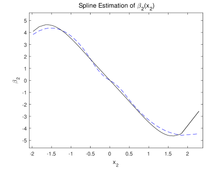
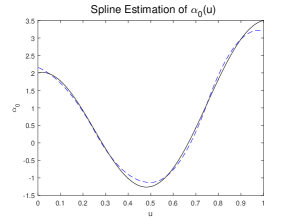
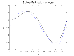
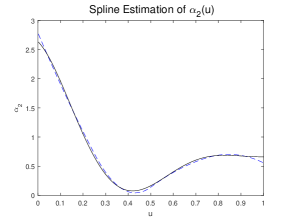
To visualize the performance of three-step estimation method, we consider T=500,K=3andI=25,formulae-sequence𝑇500𝐾3and𝐼25T=500,K=3\ \text{and}\ I=25, and approximate the unknown functions using three order B-spline functions. Figures 1 and 2 presents the estimated additive component function βk(),k=1,2,formulae-sequencesubscript𝛽𝑘𝑘12\beta_{k}\left(\cdot\right),k=1,2, and the estimated varying-coefficient functions αk(),subscript𝛼𝑘\alpha_{k}\left(\cdot\right), k=0,1,2𝑘012k=0,1,2, respectively. They both show that the proposed three-step estimation method can approximate the true function well even for a moderate sample size.

Refer to caption Refer to caption
(a) (b)
Figure 1: Estimation of additive component functions. (a) - (b) Additive component functions βk(),k=1,2formulae-sequencesubscript𝛽𝑘𝑘12\beta_{k}\left(\cdot\right),k=1,2 (solid black curve) and its estimation β^k()subscript^𝛽𝑘\hat{\beta}_{k}\left(\cdot\right) (dashed blue curve).
Refer to caption Refer to caption Refer to caption
(c) (d) (e)
Figure 2: Estimation of varying-coefficient component functions. (c) - (e)Varying-coefficient component functions αk(),k=0,1,2formulae-sequencesubscript𝛼𝑘𝑘012\alpha_{k}\left(\cdot\right),k=0,1,2 (solid black curve) and their spline estimators α^ksubscript^𝛼𝑘\hat{\alpha}_{k} (dashed blue curve).
Example 2.

We consider a varying-coefficient additive model with additive term and varying-coefficient term.

Yt,T=subscript𝑌𝑡𝑇absent\displaystyle Y_{t,T}= α0(t/T)+k=14αk(t/T)βk(Xt,T(k))+εtsubscript𝛼0𝑡𝑇superscriptsubscript𝑘14subscript𝛼𝑘𝑡𝑇subscript𝛽𝑘superscriptsubscript𝑋𝑡𝑇𝑘subscript𝜀𝑡\displaystyle\alpha_{0}\left(t/T\right)+\sum_{k=1}^{4}\alpha_{k}\left(t/T\right)\beta_{k}(X_{t,T}^{\left(k\right)})+\varepsilon_{t}
Xt,T(1)=superscriptsubscript𝑋𝑡𝑇1absent\displaystyle X_{t,T}^{\left(1\right)}= 0.7(t/T)Xt1,T(1)0.5(t/T)2Xt2,T(1)+0.5ξ1,t,0.7𝑡𝑇superscriptsubscript𝑋𝑡1𝑇10.5superscript𝑡𝑇2superscriptsubscript𝑋𝑡2𝑇10.5subscript𝜉1𝑡\displaystyle 0.7\left(t/T\right)X_{t-1,T}^{\left(1\right)}-0.5\left(t/T\right)^{2}X_{t-2,T}^{\left(1\right)}+0.5\xi_{1,t},
Xt,T(2)=superscriptsubscript𝑋𝑡𝑇2absent\displaystyle X_{t,T}^{\left(2\right)}= 0.8(t/T)Xt1,T(2)0.2(t/T)2Xt2,T(2)+0.5ξ2,t,0.8𝑡𝑇superscriptsubscript𝑋𝑡1𝑇20.2superscript𝑡𝑇2superscriptsubscript𝑋𝑡2𝑇20.5subscript𝜉2𝑡\displaystyle 0.8\left(t/T\right)X_{t-1,T}^{\left(2\right)}-0.2\left(t/T\right)^{2}X_{t-2,T}^{\left(2\right)}+0.5\xi_{2,t},
Xt,T(3)=superscriptsubscript𝑋𝑡𝑇3absent\displaystyle X_{t,T}^{\left(3\right)}= 0.6(t/T)Xt1,T(3)0.3(t/T)2Xt2,T(3)+0.5ξ3,t,0.6𝑡𝑇superscriptsubscript𝑋𝑡1𝑇30.3superscript𝑡𝑇2superscriptsubscript𝑋𝑡2𝑇30.5subscript𝜉3𝑡\displaystyle 0.6\left(t/T\right)X_{t-1,T}^{\left(3\right)}-0.3\left(t/T\right)^{2}X_{t-2,T}^{\left(3\right)}+0.5\xi_{3,t},
Xt,T(4)=superscriptsubscript𝑋𝑡𝑇4absent\displaystyle X_{t,T}^{\left(4\right)}= 0.6(t/T)Xt1,T(4)+0.5ξ4,t,0.6𝑡𝑇superscriptsubscript𝑋𝑡1𝑇40.5subscript𝜉4𝑡\displaystyle 0.6\left(t/T\right)X_{t-1,T}^{\left(4\right)}+0.5\xi_{4,t},

where {εt},subscript𝜀𝑡\{\varepsilon_{t}\}, {ξk,t},k=1,2,3,4,formulae-sequencesubscript𝜉𝑘𝑡𝑘1234\{\xi_{k,t}\},k=1,2,3,4, are iid standard normal variables and ak(u),k=0,1,2,formulae-sequencesubscript𝑎𝑘𝑢𝑘012a_{k}\left(u\right),k=0,1,2, are given in Example 1, α3(u)=1,subscript𝛼3𝑢1\alpha_{3}\left(u\right)=1,

α4(u)=subscript𝛼4𝑢absent\displaystyle\alpha_{4}\left(u\right)= {3u(1u)2+1}/3u(1u)2+1L2,3𝑢superscript1𝑢21subscriptnorm3𝑢superscript1𝑢21subscript𝐿2\displaystyle\{3u\left(1-u\right)^{2}+1\}/\parallel 3u\left(1-u\right)^{2}+1\parallel_{L_{2}},
β1(x1)=subscript𝛽1subscript𝑥1absent\displaystyle\beta_{1}\left(x_{1}\right)= 0.7sin(π2x1)0.5x1(2x1)2,0.7𝑠𝑖𝑛𝜋2subscript𝑥10.5subscript𝑥1superscript2subscript𝑥12\displaystyle 0.7sin\left(\frac{\pi}{2}x_{1}\right)-0.5x_{1}\left(2-x_{1}\right)^{2},
β2(x2)=subscript𝛽2subscript𝑥2absent\displaystyle\beta_{2}\left(x_{2}\right)= 3x2cos(π2x2)0.8sin(π2x2),3subscript𝑥2𝜋2subscript𝑥20.8𝜋2subscript𝑥2\displaystyle 3x_{2}\cos{\left(\frac{\pi}{2}x_{2}\right)}-0.8\sin{\left(\frac{\pi}{2}x_{2}\right)},

β3(x3)=2x3(1+x3)subscript𝛽3subscript𝑥32subscript𝑥31subscript𝑥3\beta_{3}\left(x_{3}\right)=2x_{3}\left(1+x_{3}\right) and β4(x4)=x4.subscript𝛽4subscript𝑥4subscript𝑥4\beta_{4}\left(x_{4}\right)=x_{4}.

To investigate the performance of the proposed two-stage model selection procedure, we take the sample size T=300,600,900,𝑇300600900T=300,600,900, segment length I=30𝐼30I=30, and the same interior knots K=3𝐾3K=3 for all univariate functions. Based on 100 replications, Table 2 lists the MISE of three-step spline estimators (UMISE), the SCAD penalized spline estimators (PMISE) and oracle estimators (OMISE) which are obtained by assuming the true model structure is known. The smoothing parameter (λT,μT)subscript𝜆𝑇subscript𝜇𝑇\left(\lambda_{T},\mu_{T}\right) is chosen according to the BIC criterion described in Section 4 and the number in parenthesis is the standard deviation of corresponding MISE.

Table 3 compares the performance of correct-fitting(C-F), over-fitting(O-F) and under-fitting(U-F) the pure varying-coefficient terms (i.e., the additive component function is linear), the pure additive terms (i.e., the varying-coefficient component function is constant) and the true model. The results show the numbers of correctly identifying additive terms, varying-coefficient terms and true model become larger as the sample size increases.

Table 2: Comparison of MISE in Example 2
T𝑇T (λT,μT)subscript𝜆𝑇subscript𝜇𝑇\left(\lambda_{T},\mu_{T}\right) Function𝐹𝑢𝑛𝑐𝑡𝑖𝑜𝑛Function UMISE PMISE OMISE
300 (0.0686,0.15)0.06860.15\left(0.0686,0.15\right) α0subscript𝛼0\alpha_{0} 0.2284 (0.1954) 0.0900(0.0615) 0.0351(0.0206)
α1subscript𝛼1\alpha_{1} 0.0378(0.0231) 0.0260(0.0166) 0.0239(0.0151)
α2subscript𝛼2\alpha_{2} 0.1419(0.0967) 0.0571(0.0406) 0.0387(0.0269)
α3subscript𝛼3\alpha_{3} 0.0104(0.0074) 0.0044(0.0081)
α4subscript𝛼4\alpha_{4} 0.1142(0.1160) 0.0729(0.0589) 0.0550(0.0358)
β1subscript𝛽1\beta_{1} 0.0340(0.0235) 0.0310(0.0224) 0.0269(0.0189)
β2subscript𝛽2\beta_{2} 0.0698(0.0455) 0.0492(0.0369) 0.0313(0.0288)
β3subscript𝛽3\beta_{3} 0.0288(0.0226) 0.0288(0.0244) 0.0265(0.0222)
β4subscript𝛽4\beta_{4} 0.0303(0.0241) 0.0167(0.0258)
600 (0.053,0.1286)0.0530.1286\left(0.053,0.1286\right) α0subscript𝛼0\alpha_{0} 0.1635 (0.1666) 0.0307(0.0201) 0.0160(0.0074)
α1subscript𝛼1\alpha_{1} 0.0114(0.0064) 0.0087(0.0054) 0.0083(0.0057)
α2subscript𝛼2\alpha_{2} 0.0769(0.0679) 0.0295(0.0199) 0.0171(0.0111)
α3subscript𝛼3\alpha_{3} 0.0074(0.0045) 0.0019(0.0039)
α4subscript𝛼4\alpha_{4} 0.0381(0.0287) 0.0312(0.0214) 0.0285(0.0207)
β1subscript𝛽1\beta_{1} 0.0195(0.0142) 0.0181(0.0127) 0.0175(0.0126)
β2subscript𝛽2\beta_{2} 0.0536(0.0365) 0.0321(0.0276) 0.0183(0.0097)
β3subscript𝛽3\beta_{3} 0.0134(0.0092) 0.0124(0.0092) 0.0121(0.0090)
β4subscript𝛽4\beta_{4} 0.0119(0.0096) 0.0049(0.0104)
900 (0.06,0.15)0.060.15\left(0.06,0.15\right) α0subscript𝛼0\alpha_{0} 0.0993 (0.1047) 0.0220(0.0177) 0.0114(0.0054)
α1subscript𝛼1\alpha_{1} 0.0111(0.0053) 0.0066(0.0034) 0.0063(0.0032)
α2subscript𝛼2\alpha_{2} 0.0409(0.0235) 0.0144(0.0108) 0.0113(0.0073)
α3subscript𝛼3\alpha_{3} 0.0046(0.0031) 0.0002(0.0012)
α4subscript𝛼4\alpha_{4} 0.0215(0.0139) 0.0205(0.0110) 0.0182(0.0113)
β1subscript𝛽1\beta_{1} 0.0150(0.0089) 0.0108(0.0068) 0.0098(0.0062)
β2subscript𝛽2\beta_{2} 0.0215(0.0118) 0.0205(0.0125) 0.0178(0.0094)
β3subscript𝛽3\beta_{3} 0.0081(0.0054) 0.0078(0.0052) 0.0075(0.0047)
β4subscript𝛽4\beta_{4} 0.0079(0.0054) 0.0015(0.0025)
Table 3: Performance of Model identification in Example 2
T𝑇T Additive terms Varying-coefficient terms True model
C-F O-F U-F C-F O-F U-F C-F O-F U-F
300 71 12 17 75 0 25 54 38 8
600 80 7 13 88 0 12 70 24 6
900 92 6 2 94 0 6 86 8 6

Appendix A Appendix

A.1 Assumption Sets

Let |𝐚|𝐚|\mathbf{a}| be the Euclidean norm of a real valued vector 𝐚.𝐚\mathbf{a}. Denote the space of l𝑙l-order smooth functions defined on [0,1]01[0,1] as C(l)[0,1]={m|m(l)C[0,1]}superscript𝐶𝑙01conditional-set𝑚superscript𝑚𝑙𝐶01C^{\left(l\right)}[0,1]=\{m|m^{\left(l\right)}\in C[0,1]\} and the class of Lipschitz continuous functions for some fixed constant C>0𝐶0C>0 as Lip([0,1],C)={m||m(x)m(x)|C|xx|,x,x[0,1]}.𝐿𝑖𝑝01𝐶conditional-set𝑚formulae-sequence𝑚𝑥𝑚superscript𝑥𝐶𝑥superscript𝑥for-all𝑥superscript𝑥01Lip\left([0,1],C\right)=\{m||m\left(x\right)-m\left(x^{\prime}\right)|\leq C|x-x^{\prime}|,\forall x,x^{\prime}\in[0,1]\}.

The necessary conditions to prove asymptotic properties are listed as below.

  • (A1)

    The process {𝐗t,T}subscript𝐗𝑡𝑇\{\mathbf{X}_{t,T}\} is stationary locally in time, that is, for each rescaled time point u[0,1],𝑢01u\in[0,1], there exists a strictly stationary process {𝐗t(u)}subscript𝐗𝑡𝑢\{\mathbf{X}_{t}\left(u\right)\} such that |𝐗t,T𝐗t(u)|{|tTu|+1T}Ut,T(u)subscript𝐗𝑡𝑇subscript𝐗𝑡𝑢𝑡𝑇𝑢1𝑇subscript𝑈𝑡𝑇𝑢|\mathbf{X}_{t,T}-\mathbf{X}_{t}\left(u\right)|\leq\{|\frac{t}{T}-u|+\frac{1}{T}\}U_{t,T}\left(u\right) a.s. with E[Ut,T(u)ρ]C𝐸delimited-[]subscript𝑈𝑡𝑇superscript𝑢𝜌𝐶E[U_{t,T}\left(u\right)^{\rho}]\leq C for some ρ2𝜌2\rho\geq 2 and C<𝐶C<\infty independent of u,t,𝑢𝑡u,t, and T.𝑇T.

  • (A2)

    At each rescaled time point u[0,1],𝑢01u\in[0,1], the joint density function fu(𝐱)subscript𝑓𝑢𝐱f_{u}\left(\mathbf{x}\right) of the stationary approximation process 𝐗t(u)subscript𝐗𝑡𝑢\mathbf{X}_{t}\left(u\right) is bounded below and above uniformly on u[0,1]::𝑢01absentu\in[0,1]:

    0<cfinf𝐱[0,1]pfu(𝐱)sup𝐱[0,1]pfu(𝐱)Cfuniformly onu[0,1].0subscript𝑐𝑓subscriptinfimum𝐱superscript01𝑝subscript𝑓𝑢𝐱subscriptsupremum𝐱superscript01𝑝subscript𝑓𝑢𝐱subscript𝐶𝑓uniformly on𝑢010<c_{f}\leq\inf_{\mathbf{x}\in[0,1]^{p}}f_{u}\left(\mathbf{x}\right)\leq\sup_{\mathbf{x}\in[0,1]^{p}}f_{u}\left(\mathbf{x}\right)\leq C_{f}\ \text{uniformly on}\ u\in[0,1].

    Meantime, 𝐗t,Tsubscript𝐗𝑡𝑇\mathbf{X}_{t,T} has density function with respective to certain measure.

  • (A3)

    εtsubscript𝜀𝑡\varepsilon_{t} iid, and Eεt=0,𝐸subscript𝜀𝑡0E\varepsilon_{t}=0, Eεt2=1.𝐸superscriptsubscript𝜀𝑡21E\varepsilon_{t}^{2}=1. Given 𝐗t,T,subscript𝐗𝑡𝑇\mathbf{X}_{t,T}, εtWN(0,1).similar-tosubscript𝜀𝑡𝑊𝑁01\varepsilon_{t}\sim WN\left(0,1\right).

  • (A4)

    There exists positive constants K0subscript𝐾0K_{0} and λ𝜆\lambda such that α(k)K0expλk𝛼𝑘subscript𝐾0superscript𝜆𝑘\alpha\left(k\right)\leq K_{0}\exp^{-\lambda k} for all k1,𝑘1k\geq 1, where α()𝛼\alpha\left(\cdot\right) is the α𝛼\alpha-mixing coefficients for process {𝒵t:=(𝐗t,Tτ,εt)τ,t=1,,T},formulae-sequenceassignsubscript𝒵𝑡superscriptsuperscriptsubscript𝐗𝑡𝑇𝜏subscript𝜀𝑡𝜏𝑡1𝑇\big{\{}\mathcal{Z}_{t}:=\left(\mathbf{X}_{t,T}^{\tau},\varepsilon_{t}\right)^{\tau},t=1,\cdots,T\big{\}}, and defined as

    α(k)=supBσ{𝒵s,st},Cσ{𝒵s,st+k}|P(BC)P(B)P(C)|,k1.formulae-sequence𝛼𝑘subscriptsupremumformulae-sequence𝐵𝜎subscript𝒵𝑠𝑠𝑡𝐶𝜎subscript𝒵𝑠𝑠𝑡𝑘𝑃𝐵𝐶𝑃𝐵𝑃𝐶𝑘1\alpha\left(k\right)=\sup_{B\in\sigma\{\mathcal{Z}_{s},s\leq t\},C\in\sigma\{\mathcal{Z}_{s},s\geq t+k\}}|P\left(B\cap C\right)-P\left(B\right)P\left(C\right)|,\ k\geq 1.
  • (A5)

    The conditional standard deviation function σ𝜎\sigma is bounded below and above uniformly on u[0,1],𝑢01u\in[0,1], i.e.,

    cσinf𝐱[0,1]pσ(u,𝐱)sup𝐱[0,1]pσ(u,𝐱)Cσuniformly onu[0,1]subscript𝑐𝜎subscriptinfimum𝐱superscript01𝑝𝜎𝑢𝐱subscriptsupremum𝐱superscript01𝑝𝜎𝑢𝐱subscript𝐶𝜎uniformly on𝑢01c_{\sigma}\leq\inf_{\mathbf{x}\in[0,1]^{p}}\sigma\left(u,\mathbf{x}\right)\leq\sup_{\mathbf{x}\in[0,1]^{p}}\sigma\left(u,\mathbf{x}\right)\leq C_{\sigma}\ \text{uniformly on}\ u\in[0,1]

    for some positive constants cσsubscript𝑐𝜎c_{\sigma} and Cσ.subscript𝐶𝜎C_{\sigma}.

  • (A6)

    αkC(dk1)[0,1]subscript𝛼𝑘superscript𝐶subscript𝑑𝑘101\alpha_{k}\in C^{\left(d_{k}-1\right)}[0,1] and αk(dk1)Lip([0,1],C1,k)superscriptsubscript𝛼𝑘subscript𝑑𝑘1𝐿𝑖𝑝01subscript𝐶1𝑘\alpha_{k}^{\left(d_{k}-1\right)}\in Lip([0,1],C_{1,k}) where dksubscript𝑑𝑘d_{k} is an integer such that 1dkqk.1subscript𝑑𝑘subscript𝑞𝑘1\leq d_{k}\leq q_{k}.

  • (A7)

    βkC(rk1)[0,1]subscript𝛽𝑘superscript𝐶subscript𝑟𝑘101\beta_{k}\in C^{\left(r_{k}-1\right)}[0,1] and βk(rk1)Lip([0,1],C2,k)superscriptsubscript𝛽𝑘subscript𝑟𝑘1𝐿𝑖𝑝01subscript𝐶2𝑘\beta_{k}^{\left(r_{k}-1\right)}\in Lip([0,1],C_{2,k}) where rksubscript𝑟𝑘r_{k} is an integer such that 1rkpk.1subscript𝑟𝑘subscript𝑝𝑘1\leq r_{k}\leq p_{k}.

  • (A8)

    The knots for αk(),k=0,,p,formulae-sequencesubscript𝛼𝑘𝑘0𝑝\alpha_{k}\left(\cdot\right),k=0,\cdots,p,

    0=ηk,1qk=0subscript𝜂𝑘1subscript𝑞𝑘absent\displaystyle 0=\eta_{k,1-q_{k}}= =ηk,0<ηk,1<<ηk,Kk,C<ηk,Kk,C+1subscript𝜂𝑘0subscript𝜂𝑘1subscript𝜂𝑘subscript𝐾𝑘𝐶subscript𝜂𝑘subscript𝐾𝑘𝐶1\displaystyle\cdots=\eta_{k,0}<\eta_{k,1}<\cdots<\eta_{k,K_{k,C}}<\eta_{k,K_{k,C}+1}
    =\displaystyle= =ηk,Kk,C+qk=1subscript𝜂𝑘subscript𝐾𝑘𝐶subscript𝑞𝑘1\displaystyle\cdots=\eta_{k,K_{k,C}+q_{k}}=1

    and the knots for βk(),k=1,,p,formulae-sequencesubscript𝛽𝑘𝑘1𝑝\beta_{k}\left(\cdot\right),k=1,\cdots,p,

    0=τk,1pk=0subscript𝜏𝑘1subscript𝑝𝑘absent\displaystyle 0=\tau_{k,1-p_{k}}= =τk,0<τk,1<<τk,Kk,A<τk,Kk,A+1subscript𝜏𝑘0subscript𝜏𝑘1subscript𝜏𝑘subscript𝐾𝑘𝐴subscript𝜏𝑘subscript𝐾𝑘𝐴1\displaystyle\cdots=\tau_{k,0}<\tau_{k,1}<\cdots<\tau_{k,K_{k,A}}<\tau_{k,K_{k,A}+1}
    =\displaystyle= =τk,Kk,A+pk=1subscript𝜏𝑘subscript𝐾𝑘𝐴subscript𝑝𝑘1\displaystyle\cdots=\tau_{k,K_{k,A}+p_{k}}=1

    has bounded mesh ratio:

    lim supTmax0kpmax1lKk,C+1{ηk,lηk,l1}min1lKk,C+1{ηk,lηk,l1}<.subscriptlimit-supremum𝑇subscript0𝑘𝑝subscript1𝑙subscript𝐾𝑘𝐶1subscript𝜂𝑘𝑙subscript𝜂𝑘𝑙1subscript1𝑙subscript𝐾𝑘𝐶1subscript𝜂𝑘𝑙subscript𝜂𝑘𝑙1\limsup_{T\to\infty}\max_{0\leq k\leq p}\frac{\max_{1\leq l\leq K_{k,C}+1}\{\eta_{k,l}-\eta_{k,l-1}\}}{\min_{1\leq l\leq K_{k,C}+1}\{\eta_{k,l}-\eta_{k,l-1}\}}<\infty.
    lim supTmax1kpmax1lKk,A+1{τk,lτk,l1}min1lKk,A+1{τk,lτk,l1}<,subscriptlimit-supremum𝑇subscript1𝑘𝑝subscript1𝑙subscript𝐾𝑘𝐴1subscript𝜏𝑘𝑙subscript𝜏𝑘𝑙1subscript1𝑙subscript𝐾𝑘𝐴1subscript𝜏𝑘𝑙subscript𝜏𝑘𝑙1\limsup_{T\to\infty}\max_{1\leq k\leq p}\frac{\max_{1\leq l\leq K_{k,A}+1}\{\tau_{k,l}-\tau_{k,l-1}\}}{\min_{1\leq l\leq K_{k,A}+1}\{\tau_{k,l}-\tau_{k,l-1}\}}<\infty,
  • (A9)

    lim supT(KA/min1kpKk,A)<subscriptlimit-supremum𝑇subscript𝐾𝐴subscript1𝑘𝑝subscript𝐾𝑘𝐴\limsup_{T\to\infty}\left(K_{A}/\min_{1\leq k\leq p}K_{k,A}\right)<\infty, KA/T0,subscript𝐾𝐴𝑇0K_{A}/T\to 0, KAlogT/T0subscript𝐾𝐴𝑇𝑇0K_{A}\log{T}/\sqrt{T}\to 0 and TKA.𝑇subscript𝐾𝐴\sqrt{T}K_{A}\to\infty.

  • (A10)

    lim supT(KC/min0kpKk,C)<subscriptlimit-supremum𝑇subscript𝐾𝐶subscript0𝑘𝑝subscript𝐾𝑘𝐶\limsup_{T\to\infty}\left(K_{C}/\min_{0\leq k\leq p}K_{k,C}\right)<\infty and KC/T0.subscript𝐾𝐶𝑇0K_{C}/T\to 0.

Remark 7: Assumption (A1) specifies a data generating process (GDP). Assumptions (A2) - (A5) are standard in time-series context, see [39, 40]. Assumptions (A6) - (A8) are common in typical spline approximation literature, for instance, [48].

A.2 Proofs for Main Theorems

Firstly, we need some lemmas before proving main theorems. Let 𝐠=(g1,,gp)τ𝐠superscriptsubscript𝑔1subscript𝑔𝑝𝜏\mathbf{g}=\left(g_{1},\cdots,g_{p}\right)^{\tau} and 𝐡=(h1,,hp)τ𝐡superscriptsubscript1subscript𝑝𝜏\mathbf{h}=\left(h_{1},\cdots,h_{p}\right)^{\tau} be any two-vector valued function. Define empirical inner product

𝐠,𝐡T=1Tt=1Tk=1pgk(Xt,T(k))hk(Xt,T(k)),subscript𝐠𝐡𝑇1𝑇superscriptsubscript𝑡1𝑇superscriptsubscript𝑘1𝑝subscript𝑔𝑘superscriptsubscript𝑋𝑡𝑇𝑘subscript𝑘superscriptsubscript𝑋𝑡𝑇𝑘\langle\mathbf{g},\mathbf{h}\rangle_{T}=\frac{1}{T}\sum_{t=1}^{T}\sum_{k=1}^{p}g_{k}\left(X_{t,T}^{\left(k\right)}\right)h_{k}\left(X_{t,T}^{\left(k\right)}\right),

and theoretical inner product

𝐠,𝐡=k=1p01E[gk(Xt(k)(u))hk(Xt(k)(u))]du,𝐠𝐡superscriptsubscript𝑘1𝑝superscriptsubscript01𝐸delimited-[]subscript𝑔𝑘superscriptsubscript𝑋𝑡𝑘𝑢subscript𝑘superscriptsubscript𝑋𝑡𝑘𝑢differential-d𝑢\langle\mathbf{g},\mathbf{h}\rangle=\sum_{k=1}^{p}\int_{0}^{1}E\big{[}g_{k}\left(X_{t}^{\left(k\right)}\left(u\right)\right)h_{k}\left(X_{t}^{\left(k\right)}\left(u\right)\right)\big{]}\mathrm{d}u,

Denote the induced norm by 𝐠,𝐡Tsubscript𝐠𝐡𝑇\langle\mathbf{g},\mathbf{h}\rangle_{T} and 𝐠,𝐡𝐠𝐡\langle\mathbf{g},\mathbf{h}\rangle as T\parallel\cdot\parallel_{T} and ,\parallel\cdot\parallel, respectively. In addition to, 𝐠L22=k=1pgkL22.superscriptsubscriptnorm𝐠subscript𝐿22superscriptsubscript𝑘1𝑝superscriptsubscriptnormsubscript𝑔𝑘subscript𝐿22\parallel\mathbf{g}\parallel_{L_{2}}^{2}=\sum_{k=1}^{p}\parallel g_{k}\parallel_{L_{2}}^{2}. Given sequences of positive numbers ansubscript𝑎𝑛a_{n} and bn,subscript𝑏𝑛b_{n}, anbnprecedes-or-equalssubscript𝑎𝑛subscript𝑏𝑛a_{n}\preceq b_{n} means an/bnsubscript𝑎𝑛subscript𝑏𝑛a_{n}/b_{n} is bounded and anbnasymptotically-equalssubscript𝑎𝑛subscript𝑏𝑛a_{n}\asymp b_{n} means anbnprecedes-or-equalssubscript𝑎𝑛subscript𝑏𝑛a_{n}\preceq b_{n} and bnanprecedes-or-equalssubscript𝑏𝑛subscript𝑎𝑛b_{n}\preceq a_{n} hold.

Lemma 1.

Let gk(zk)=l=1Jk,Aγklψkl(zk)subscript𝑔𝑘subscript𝑧𝑘superscriptsubscript𝑙1subscript𝐽𝑘𝐴subscript𝛾𝑘𝑙subscript𝜓𝑘𝑙subscript𝑧𝑘g_{k}\left(z_{k}\right)=\sum_{l=1}^{J_{k,A}}\gamma_{kl}\psi_{kl}\left(z_{k}\right) and γk=(γk1,,γkJk,A)τsubscript𝛾𝑘superscriptsubscript𝛾𝑘1subscript𝛾𝑘subscript𝐽𝑘𝐴𝜏\gamma_{k}=\left(\gamma_{k1},\cdots,\gamma_{kJ_{k,A}}\right)^{\tau} for k=1,,p.𝑘1𝑝k=1,\cdots,p. Denote γ=(γ1τ,,γpτ)τ𝛾superscriptsuperscriptsubscript𝛾1𝜏superscriptsubscript𝛾𝑝𝜏𝜏\mathbf{\gamma}=\left(\gamma_{1}^{\tau},\cdots,\gamma_{p}^{\tau}\right)^{\tau} and 𝐠(𝐳)=(g1(z1),,gp(zp))τ.𝐠𝐳superscriptsubscript𝑔1subscript𝑧1subscript𝑔𝑝subscript𝑧𝑝𝜏\mathbf{g}\left(\mathbf{z}\right)=\left(g_{1}\left(z_{1}\right),\cdots,g_{p}\left(z_{p}\right)\right)^{\tau}. Then 𝐠2𝐠L22|γ|2asymptotically-equalssuperscriptnorm𝐠2superscriptsubscriptnorm𝐠subscript𝐿22asymptotically-equalssuperscript𝛾2\parallel\mathbf{g}\parallel^{2}\asymp\parallel\mathbf{g}\parallel_{L_{2}}^{2}\asymp|\mathbf{\gamma}|^{2} holds under Assumption (A2).

Proof.

In combination with Assumption (A2) and the property (iv) of {ψkl},subscript𝜓𝑘𝑙\{\psi_{kl}\}, we have

𝐠2=superscriptnorm𝐠2absent\displaystyle\parallel\mathbf{g}\parallel^{2}= k=1p01E[gk2(Xt(k)(u))]du=k=1p01E[l=1Jk,Aγklψkl(Xt(k)(u))]2dusuperscriptsubscript𝑘1𝑝superscriptsubscript01𝐸delimited-[]superscriptsubscript𝑔𝑘2superscriptsubscript𝑋𝑡𝑘𝑢differential-d𝑢superscriptsubscript𝑘1𝑝superscriptsubscript01𝐸superscriptdelimited-[]superscriptsubscript𝑙1subscript𝐽𝑘𝐴subscript𝛾𝑘𝑙subscript𝜓𝑘𝑙superscriptsubscript𝑋𝑡𝑘𝑢2differential-d𝑢\displaystyle\sum_{k=1}^{p}\int_{0}^{1}E\big{[}g_{k}^{2}(X_{t}^{\left(k\right)}\left(u\right))\big{]}\mathrm{d}u=\sum_{k=1}^{p}\int_{0}^{1}E\big{[}\sum_{l=1}^{J_{k,A}}\gamma_{kl}\psi_{kl}(X_{t}^{\left(k\right)}\left(u\right))\big{]}^{2}\mathrm{d}u
asymptotically-equals\displaystyle\asymp k=1p01gkL22du=𝐠L22k=1p|γk|2=|γ|2superscriptsubscript𝑘1𝑝superscriptsubscript01subscriptsuperscriptnormsubscript𝑔𝑘2subscript𝐿2differential-d𝑢superscriptsubscriptnorm𝐠subscript𝐿22asymptotically-equalssuperscriptsubscript𝑘1𝑝superscriptsubscript𝛾𝑘2superscript𝛾2\displaystyle\sum_{k=1}^{p}\int_{0}^{1}\parallel g_{k}\parallel^{2}_{L_{2}}\mathrm{d}u=\parallel\mathbf{g}\parallel_{L_{2}}^{2}\asymp\sum_{k=1}^{p}|\gamma_{k}|^{2}=|\mathbf{\gamma}|^{2}

Lemma 2.

Let 𝒢𝒢\mathcal{G} be the collection of vector valued functions 𝐠=(g1,,gp)τ𝐠superscriptsubscript𝑔1subscript𝑔𝑝𝜏\mathbf{g}=\left(g_{1},\cdots,g_{p}\right)^{\tau} with gkGksubscript𝑔𝑘subscript𝐺𝑘g_{k}\in G_{k} such that gkL2<subscriptnormsubscript𝑔𝑘subscript𝐿2\parallel g_{k}\parallel_{L_{2}}<\infty for k=1,,p,𝑘1𝑝k=1,\cdots,p, where Gksubscript𝐺𝑘G_{k} is defined in Section 5.1. Then under Assumption (A1), (A2), (A4) and (A9), as T,𝑇T\to\infty,

sup𝐠1,𝐠2𝒢|𝐠1,𝐠2T𝐠2,𝐠2|𝐠1𝐠2=Op(KAlogTT)=op(1).subscriptsupremumsubscript𝐠1subscript𝐠2𝒢subscriptsubscript𝐠1subscript𝐠2𝑇subscript𝐠2subscript𝐠2normsubscript𝐠1normsubscript𝐠2subscript𝑂𝑝subscript𝐾𝐴𝑇𝑇subscript𝑜𝑝1\sup_{\mathbf{g}_{1},\mathbf{g}_{2}\in\mathcal{G}}\frac{|\langle\mathbf{g}_{1},\mathbf{g}_{2}\rangle_{T}-\langle\mathbf{g}_{2},\mathbf{g}_{2}\rangle|}{\parallel\mathbf{g}_{1}\parallel\cdot\parallel\mathbf{g}_{2}\parallel}=O_{p}\left(\frac{K_{A}\log{T}}{T}\right)=o_{p}\left(1\right).
Proof.

For any 𝐠(i)=(g1(i),,gp(i))τ𝒢,i=1,2,formulae-sequencesuperscript𝐠𝑖superscriptsuperscriptsubscript𝑔1𝑖superscriptsubscript𝑔𝑝𝑖𝜏𝒢𝑖12\mathbf{g}^{\left(i\right)}=(g_{1}^{\left(i\right)},\cdots,g_{p}^{\left(i\right)})^{\tau}\in\mathcal{G},i=1,2, there exists coefficients γkl(1)superscriptsubscript𝛾𝑘𝑙1\gamma_{kl}^{\left(1\right)} and γkl(2),superscriptsubscript𝛾𝑘𝑙2\gamma_{kl}^{\left(2\right)}, l=1,,Jk,A,k=1,,p,formulae-sequence𝑙1subscript𝐽𝑘𝐴𝑘1𝑝l=1,\cdots,J_{k,A},k=1,\cdots,p, such that

𝐠k(1)(zk)=l=1Jk,Aγkl(1)ψkl(zk)and𝐠k(2)(zk)=l=1Jk,Aγkl(2)ψkl(zk)formulae-sequencesubscriptsuperscript𝐠1𝑘subscript𝑧𝑘superscriptsubscript𝑙1subscript𝐽𝑘𝐴superscriptsubscript𝛾𝑘𝑙1subscript𝜓𝑘𝑙subscript𝑧𝑘andsubscriptsuperscript𝐠2𝑘subscript𝑧𝑘superscriptsubscript𝑙1subscript𝐽𝑘𝐴superscriptsubscript𝛾𝑘𝑙2subscript𝜓𝑘𝑙subscript𝑧𝑘\mathbf{g}^{\left(1\right)}_{k}\left(z_{k}\right)=\sum_{l=1}^{J_{k,A}}\gamma_{kl}^{\left(1\right)}\psi_{kl}\left(z_{k}\right)\ \ \text{and}\ \ \mathbf{g}^{\left(2\right)}_{k}\left(z_{k}\right)=\sum_{l=1}^{J_{k,A}}\gamma_{kl}^{\left(2\right)}\psi_{kl}\left(z_{k}\right)

for k=1,,p.𝑘1𝑝k=1,\cdots,p. It is not difficult to see that

|𝐠1,𝐠2T𝐠1,𝐠2|k=1pl,l=1Jk,A|γkl(1)γkl(2)||ψkl,ψklTψkl,ψkl|.subscriptsubscript𝐠1subscript𝐠2𝑇subscript𝐠1subscript𝐠2superscriptsubscript𝑘1𝑝superscriptsubscript𝑙superscript𝑙1subscript𝐽𝑘𝐴superscriptsubscript𝛾𝑘𝑙1superscriptsubscript𝛾𝑘superscript𝑙2subscriptsubscript𝜓𝑘𝑙subscript𝜓𝑘superscript𝑙𝑇subscript𝜓𝑘𝑙subscript𝜓𝑘superscript𝑙|\langle\mathbf{g}_{1},\mathbf{g}_{2}\rangle_{T}-\langle\mathbf{g}_{1},\mathbf{g}_{2}\rangle|\leq\sum_{k=1}^{p}\sum_{l,l^{\prime}=1}^{J_{k,A}}|\gamma_{kl}^{\left(1\right)}\gamma_{kl^{\prime}}^{\left(2\right)}|\cdot|\langle\psi_{kl},\psi_{kl^{\prime}}\rangle_{T}-\langle\psi_{kl},\psi_{kl^{\prime}}\rangle|.

For any given k=1,,p,𝑘1𝑝k=1,\cdots,p, let lAk(l)superscript𝑙subscript𝐴𝑘𝑙l^{\prime}\in A_{k}\left(l\right) if the intersection of the supports of ψklsubscript𝜓𝑘𝑙\psi_{kl} and ψklsubscript𝜓𝑘superscript𝑙\psi_{kl^{\prime}} contains an open interval. That is, ψkl,ψklT=ψkl,ψkl=0subscriptsubscript𝜓𝑘𝑙subscript𝜓𝑘superscript𝑙𝑇subscript𝜓𝑘𝑙subscript𝜓𝑘superscript𝑙0\langle\psi_{kl},\psi_{kl^{\prime}}\rangle_{T}=\langle\psi_{kl},\psi_{kl^{\prime}}\rangle=0 if lAk(l).superscript𝑙subscript𝐴𝑘𝑙l^{\prime}\notin A_{k}\left(l\right). Moreover, it is known #{Ak(l)}C#subscript𝐴𝑘𝑙𝐶\#\{A_{k}\left(l\right)\}\leq C for some constant C𝐶C and all l,k.𝑙𝑘l,k. Moveover, for any given k,l𝑘𝑙k,l and lAk(l),superscript𝑙subscript𝐴𝑘𝑙l^{\prime}\in A_{k}\left(l\right), we have

|ψkl,ψklTψkl,ψkl|subscriptsubscript𝜓𝑘𝑙subscript𝜓𝑘superscript𝑙𝑇subscript𝜓𝑘𝑙subscript𝜓𝑘superscript𝑙\displaystyle|\langle\psi_{kl},\psi_{kl^{\prime}}\rangle_{T}-\langle\psi_{kl},\psi_{kl^{\prime}}\rangle|
=\displaystyle= |T1t=1Tψkl(Xt,T(k))ψkl(Xt,T(k))01E[ψkl(Xt(k)(u))ψkl(Xt(k)(u))]du|superscript𝑇1superscriptsubscript𝑡1𝑇subscript𝜓𝑘𝑙superscriptsubscript𝑋𝑡𝑇𝑘subscript𝜓𝑘superscript𝑙superscriptsubscript𝑋𝑡𝑇𝑘superscriptsubscript01𝐸delimited-[]subscript𝜓𝑘𝑙superscriptsubscript𝑋𝑡𝑘𝑢subscript𝜓𝑘superscript𝑙superscriptsubscript𝑋𝑡𝑘𝑢differential-d𝑢\displaystyle|T^{-1}\sum_{t=1}^{T}\psi_{kl}(X_{t,T}^{\left(k\right)})\psi_{kl^{\prime}}(X_{t,T}^{\left(k\right)})-\int_{0}^{1}E[\psi_{kl}(X_{t}^{\left(k\right)}\left(u\right))\psi_{kl^{\prime}}(X_{t}^{\left(k\right)}\left(u\right))]\mathrm{d}u|
\displaystyle\leq T1t=1T|ψkl(Xt,T(k))ψkl(Xt,T(k))ψkl(Xt(k)(t/T))ψkl(Xt(k)(t/T))|superscript𝑇1superscriptsubscript𝑡1𝑇subscript𝜓𝑘𝑙superscriptsubscript𝑋𝑡𝑇𝑘subscript𝜓𝑘superscript𝑙superscriptsubscript𝑋𝑡𝑇𝑘subscript𝜓𝑘𝑙superscriptsubscript𝑋𝑡𝑘𝑡𝑇subscript𝜓𝑘superscript𝑙superscriptsubscript𝑋𝑡𝑘𝑡𝑇\displaystyle T^{-1}\sum_{t=1}^{T}|\psi_{kl}(X_{t,T}^{\left(k\right)})\psi_{kl^{\prime}}(X_{t,T}^{\left(k\right)})-\psi_{kl}(X_{t}^{\left(k\right)}(t/T))\psi_{kl^{\prime}}(X_{t}^{\left(k\right)}(t/T))|
+\displaystyle+ T1t=1T|ψkl(Xt(k)(t/T))ψkl(Xt(k)(t/T))E[ψkl(Xt(k)(t/T))ψkl(Xt(k)(t/T))]|superscript𝑇1superscriptsubscript𝑡1𝑇subscript𝜓𝑘𝑙superscriptsubscript𝑋𝑡𝑘𝑡𝑇subscript𝜓𝑘superscript𝑙superscriptsubscript𝑋𝑡𝑘𝑡𝑇𝐸delimited-[]subscript𝜓𝑘𝑙superscriptsubscript𝑋𝑡𝑘𝑡𝑇subscript𝜓𝑘superscript𝑙superscriptsubscript𝑋𝑡𝑘𝑡𝑇\displaystyle T^{-1}\sum_{t=1}^{T}|\psi_{kl}(X_{t}^{\left(k\right)}(t/T))\psi_{kl^{\prime}}(X_{t}^{\left(k\right)}(t/T))-E[\psi_{kl}(X_{t}^{\left(k\right)}(t/T))\psi_{kl^{\prime}}(X_{t}^{\left(k\right)}(t/T))]|
+\displaystyle+ |T1t=1TE[ψkl(Xt(k)(t/T))ψkl(Xt(k)(t/T))]01E[ψkl(Xt(k)(u))ψkl(Xt(k)(u))]du|.superscript𝑇1superscriptsubscript𝑡1𝑇𝐸delimited-[]subscript𝜓𝑘𝑙superscriptsubscript𝑋𝑡𝑘𝑡𝑇subscript𝜓𝑘superscript𝑙superscriptsubscript𝑋𝑡𝑘𝑡𝑇superscriptsubscript01𝐸delimited-[]subscript𝜓𝑘𝑙superscriptsubscript𝑋𝑡𝑘𝑢subscript𝜓𝑘superscript𝑙superscriptsubscript𝑋𝑡𝑘𝑢differential-d𝑢\displaystyle|T^{-1}\sum_{t=1}^{T}E[\psi_{kl}(X_{t}^{\left(k\right)}\left(t/T\right))\psi_{kl^{\prime}}(X_{t}^{\left(k\right)}\left(t/T\right))]-\int_{0}^{1}E[\psi_{kl}(X_{t}^{\left(k\right)}\left(u\right))\psi_{kl^{\prime}}(X_{t}^{\left(k\right)}\left(u\right))]\mathrm{d}u|.

By Assumption (A1) and the boundness of B-spline, the first term above is bounded by Op(KA/T).subscript𝑂𝑝subscript𝐾𝐴𝑇O_{p}\left(K_{A}/T\right). Employing Berstein’s inequality, the second term is bounded by Op(KAlogT/T).subscript𝑂𝑝subscript𝐾𝐴𝑇𝑇O_{p}(K_{A}\log{T}/\sqrt{T}). The last term is bounded by O(1/T)𝑂1𝑇O\left(1/T\right) from the integral theory. Therefore, using Cauchy-Schwartz inequality and Assumption (A9), we obtain that

|𝐠1,𝐠2T𝐠1,𝐠2|=subscriptsubscript𝐠1subscript𝐠2𝑇subscript𝐠1subscript𝐠2absent\displaystyle|\langle\mathbf{g}_{1},\mathbf{g}_{2}\rangle_{T}-\langle\mathbf{g}_{1},\mathbf{g}_{2}\rangle|= Op(KAlogT/T)k=1pl,l|γkl(1)||γkl(2)|I(lAk(l))subscript𝑂𝑝subscript𝐾𝐴𝑇𝑇superscriptsubscript𝑘1𝑝subscript𝑙superscript𝑙superscriptsubscript𝛾𝑘𝑙1superscriptsubscript𝛾𝑘superscript𝑙2𝐼superscript𝑙subscript𝐴𝑘𝑙\displaystyle O_{p}\left(K_{A}\log{T}/\sqrt{T}\right)\sum_{k=1}^{p}\sum_{l,l^{\prime}}|\gamma_{kl}^{\left(1\right)}|\cdot|\gamma_{kl^{\prime}}^{\left(2\right)}|I\left(l^{\prime}\in A_{k}\left(l\right)\right)
=\displaystyle= Op(KAlogT/T)|γ(1)||γ(2)|,subscript𝑂𝑝subscript𝐾𝐴𝑇𝑇superscript𝛾1superscript𝛾2\displaystyle O_{p}\left(K_{A}\log{T}/\sqrt{T}\right)|\mathbf{\gamma}^{\left(1\right)}|\cdot|\mathbf{\gamma}^{\left(2\right)}|,

where γ(1)superscript𝛾1\mathbf{\gamma}^{\left(1\right)} and γ(2)superscript𝛾2\mathbf{\gamma}^{\left(2\right)} denote the vectors with entries γkl(1)superscriptsubscript𝛾𝑘𝑙1\gamma_{kl}^{\left(1\right)} and γkl(2),superscriptsubscript𝛾𝑘𝑙2\gamma_{kl}^{\left(2\right)}, respectively. By Lemma 1, we see |γ(i)|𝐠i,i=1,2formulae-sequenceasymptotically-equalssuperscript𝛾𝑖normsubscript𝐠𝑖𝑖12|\mathbf{\gamma}^{\left(i\right)}|\asymp\parallel\mathbf{g}_{i}\parallel,i=1,2 which completes the proof. ∎

Lemma 3.

Under Assumption (A1), (A2) (A4) and (A9), as T,𝑇T\to\infty,

  • (i)

    For each s=1,,NT,𝑠1subscript𝑁𝑇s=1,\cdots,N_{T}, IT1t=1ITVstVstτsuperscriptsubscript𝐼𝑇1superscriptsubscript𝑡1subscript𝐼𝑇subscript𝑉𝑠𝑡superscriptsubscript𝑉𝑠𝑡𝜏I_{T}^{-1}\sum_{t=1}^{I_{T}}V_{st}V_{st}^{\tau} has eigenvalues bounded away from 0 and \infty with probability tending to one;

  • (ii)

    T1t=1TΨk(Xt,T(k))Ψkτ(Xt,T(k))superscript𝑇1superscriptsubscript𝑡1𝑇subscriptΨ𝑘superscriptsubscript𝑋𝑡𝑇𝑘superscriptsubscriptΨ𝑘𝜏superscriptsubscript𝑋𝑡𝑇𝑘T^{-1}\sum_{t=1}^{T}\Psi_{k}(X_{t,T}^{\left(k\right)})\Psi_{k}^{\tau}(X_{t,T}^{\left(k\right)}) has eigenvalues bounded away from 0 and ,\infty, with probability tending to one.

Proof.

We only show (ii), the proof of (i) is similar. For any given vector γ=(γ1τ,,γpτ)τ𝛾superscriptsuperscriptsubscript𝛾1𝜏superscriptsubscript𝛾𝑝𝜏𝜏\mathbf{\gamma}=\left(\gamma_{1}^{\tau},\cdots,\gamma_{p}^{\tau}\right)^{\tau} with γk=(γk1,,γkJk,A)τ,subscript𝛾𝑘superscriptsubscript𝛾𝑘1subscript𝛾𝑘subscript𝐽𝑘𝐴𝜏\gamma_{k}=\left(\gamma_{k1},\cdots,\gamma_{kJ_{k,A}}\right)^{\tau}, k=1,,p,𝑘1𝑝k=1,\cdots,p, let gk(zk)=l=1Jk,Aγklψkl(zk)subscript𝑔𝑘subscript𝑧𝑘superscriptsubscript𝑙1subscript𝐽𝑘𝐴subscript𝛾𝑘𝑙subscript𝜓𝑘𝑙subscript𝑧𝑘g_{k}\left(z_{k}\right)=\sum_{l=1}^{J_{k,A}}\gamma_{kl}\psi_{kl}\left(z_{k}\right) and 𝐠(𝐳)=(g1(z1),,gp(zp))τ,𝐠𝐳superscriptsubscript𝑔1subscript𝑧1subscript𝑔𝑝subscript𝑧𝑝𝜏\mathbf{g}\left(\mathbf{z}\right)=\left(g_{1}\left(z_{1}\right),\cdots,g_{p}\left(z_{p}\right)\right)^{\tau}, where 𝐳=(z1,,zp).𝐳subscript𝑧1subscript𝑧𝑝\mathbf{z}=\left(z_{1},\cdots,z_{p}\right). Denote Ψ~(𝐳)=(Ψ1τ(z1),,Ψpτ(zp))τ,~Ψ𝐳superscriptsuperscriptsubscriptΨ1𝜏subscript𝑧1superscriptsubscriptΨ𝑝𝜏subscript𝑧𝑝𝜏\tilde{\Psi}\left(\mathbf{z}\right)=\left(\Psi_{1}^{\tau}\left(z_{1}\right),\cdots,\Psi_{p}^{\tau}\left(z_{p}\right)\right)^{\tau}, then by Lemma 1 and 2,

T1γτΨ~{𝐗t,T}Ψ~τ{𝐗t,T}γ=𝐠T2𝐠2|γ|2,superscript𝑇1superscript𝛾𝜏~Ψsubscript𝐗𝑡𝑇superscript~Ψ𝜏subscript𝐗𝑡𝑇𝛾superscriptsubscriptnorm𝐠𝑇2asymptotically-equalssuperscriptnorm𝐠2asymptotically-equalssuperscript𝛾2T^{-1}\mathbf{\gamma}^{\tau}\tilde{\Psi}\{\mathbf{X}_{t,T}\}\tilde{\Psi}^{\tau}\{\mathbf{X}_{t,T}\}\mathbf{\gamma}=\parallel\mathbf{g}\parallel_{T}^{2}\asymp\parallel\mathbf{g}\parallel^{2}\asymp|\mathbf{\gamma}|^{2},

which implies T1t=1TΨ~{𝐗t,T}Ψ~τ{𝐗t,T}superscript𝑇1superscriptsubscript𝑡1𝑇~Ψsubscript𝐗𝑡𝑇superscript~Ψ𝜏subscript𝐗𝑡𝑇T^{-1}\sum_{t=1}^{T}\tilde{\Psi}\{\mathbf{X}_{t,T}\}\tilde{\Psi}^{\tau}\{\mathbf{X}_{t,T}\} has eigenvalues bounded away from 0 and .\infty. Therefore, T1t=1TΨk{Xt,T(k)}Ψkτ{Xt,T(k)}superscript𝑇1superscriptsubscript𝑡1𝑇subscriptΨ𝑘superscriptsubscript𝑋𝑡𝑇𝑘subscriptsuperscriptΨ𝜏𝑘superscriptsubscript𝑋𝑡𝑇𝑘T^{-1}\sum_{t=1}^{T}\Psi_{k}\{X_{t,T}^{\left(k\right)}\}\Psi^{\tau}_{k}\{X_{t,T}^{\left(k\right)}\} also has eigenvalues bounded away from 0 and .\infty.

Proof for Proposition 1.
Let Vsj={1,ψ11(Xtsj,T(1)),,ψ1J1,A(Xtsj,T(1)),,ψpJp,A(Xtsj,T(p))}τ,subscript𝑉𝑠𝑗superscript1subscript𝜓11superscriptsubscript𝑋subscript𝑡𝑠𝑗𝑇1subscript𝜓1subscript𝐽1𝐴superscriptsubscript𝑋subscript𝑡𝑠𝑗𝑇1subscript𝜓𝑝subscript𝐽𝑝𝐴superscriptsubscript𝑋subscript𝑡𝑠𝑗𝑇𝑝𝜏V_{sj}=\big{\{}1,\psi_{11}(X_{t_{sj},T}^{\left(1\right)}),\cdots,\psi_{1J_{1,A}}(X_{t_{sj},T}^{\left(1\right)}),\cdots,\psi_{pJ_{p,A}}(X_{t_{sj},T}^{\left(p\right)})\big{\}}^{\tau}, then

α^s=(C^0s,h^1(s)τ,,h^p(s)τ)τ={j=1ITVsjVsjτ}1j=1ITVsjYtsj.subscript^𝛼𝑠superscriptsubscript^𝐶0𝑠superscriptsubscript^1𝑠𝜏superscriptsubscript^𝑝𝑠𝜏𝜏superscriptsuperscriptsubscript𝑗1subscript𝐼𝑇subscript𝑉𝑠𝑗superscriptsubscript𝑉𝑠𝑗𝜏1superscriptsubscript𝑗1subscript𝐼𝑇subscript𝑉𝑠𝑗subscript𝑌subscript𝑡𝑠𝑗\mathbf{\hat{\alpha}}_{s}=\left(\hat{C}_{0s},\hat{h}_{1}^{\left(s\right)\tau},\cdots,\hat{h}_{p}^{\left(s\right)\tau}\right)^{\tau}=\Big{\{}\sum_{j=1}^{I_{T}}V_{sj}V_{sj}^{\tau}\Big{\}}^{-1}\sum_{j=1}^{I_{T}}V_{sj}Y_{t_{sj}}.

Define ωs(𝐱)=C0s+k=1pβk(s)(xk),subscript𝜔𝑠𝐱subscript𝐶0𝑠superscriptsubscript𝑘1𝑝superscriptsubscript𝛽𝑘𝑠subscript𝑥𝑘\omega_{s}\left(\mathbf{x}\right)=C_{0s}+\sum_{k=1}^{p}\beta_{k}^{\left(s\right)}\left(x_{k}\right), ωs,j=ωs(𝐗tsj)subscript𝜔𝑠𝑗subscript𝜔𝑠subscript𝐗subscript𝑡𝑠𝑗\omega_{s,j}=\omega_{s}(\mathbf{X}_{t_{sj}}) and

α~s={C~0s,h~1(s)τ,,h~p(s)τ}τ={j=1ITVsjVsjτ}1j=1ITVsjωs,j.subscript~𝛼𝑠superscriptsubscript~𝐶0𝑠superscriptsubscript~1𝑠𝜏superscriptsubscript~𝑝𝑠𝜏𝜏superscriptsuperscriptsubscript𝑗1subscript𝐼𝑇subscript𝑉𝑠𝑗superscriptsubscript𝑉𝑠𝑗𝜏1superscriptsubscript𝑗1subscript𝐼𝑇subscript𝑉𝑠𝑗subscript𝜔𝑠𝑗\mathbf{\tilde{\alpha}}_{s}=\{\tilde{C}_{0s},\tilde{h}_{1}^{\left(s\right)\tau},\cdots,\tilde{h}_{p}^{\left(s\right)\tau}\}^{\tau}=\Big{\{}\sum\limits_{j=1}^{I_{T}}V_{sj}V_{sj}^{\tau}\Big{\}}^{-1}\sum\limits_{j=1}^{I_{T}}V_{sj}\omega_{s,j}.

Denote

β~k(s)(xk)=Ψk(xk)τh~k(s),βˇk(s)(xk)=Ψk(xk)τh^k(s),formulae-sequencesuperscriptsubscript~𝛽𝑘𝑠subscript𝑥𝑘subscriptΨ𝑘superscriptsubscript𝑥𝑘𝜏superscriptsubscript~𝑘𝑠subscriptsuperscriptˇ𝛽𝑠𝑘subscript𝑥𝑘subscriptΨ𝑘superscriptsubscript𝑥𝑘𝜏superscriptsubscript^𝑘𝑠\tilde{\beta}_{k}^{\left(s\right)}\left(x_{k}\right)=\Psi_{k}\left(x_{k}\right)^{\tau}\tilde{h}_{k}^{\left(s\right)},\ \ \ \ \check{\beta}^{\left(s\right)}_{k}\left(x_{k}\right)=\Psi_{k}\left(x_{k}\right)^{\tau}\hat{h}_{k}^{\left(s\right)},

and γ~k(xk)=1NTt=1NTβ~k(s)(xk),subscript~𝛾𝑘subscript𝑥𝑘1subscript𝑁𝑇superscriptsubscript𝑡1subscript𝑁𝑇superscriptsubscript~𝛽𝑘𝑠subscript𝑥𝑘\tilde{\gamma}_{k}\left(x_{k}\right)=\frac{1}{N_{T}}\sum_{t=1}^{N_{T}}\tilde{\beta}_{k}^{\left(s\right)}\left(x_{k}\right), γˇk(xk)=1NTs=1NTβˇk(s)(xk).subscriptˇ𝛾𝑘subscript𝑥𝑘1subscript𝑁𝑇superscriptsubscript𝑠1subscript𝑁𝑇subscriptsuperscriptˇ𝛽𝑠𝑘subscript𝑥𝑘\check{\gamma}_{k}\left(x_{k}\right)=\frac{1}{N_{T}}\sum_{s=1}^{N_{T}}\check{\beta}^{\left(s\right)}_{k}\left(x_{k}\right). Note that γ^k(xk)=γˇk(xk)γˇk(0),subscript^𝛾𝑘subscript𝑥𝑘subscriptˇ𝛾𝑘subscript𝑥𝑘subscriptˇ𝛾𝑘0\hat{\gamma}_{k}\left(x_{k}\right)=\check{\gamma}_{k}\left(x_{k}\right)-\check{\gamma}_{k}\left(0\right), by Cauchy-Schwartz inequality, we have

γ^kγkL22subscriptsuperscriptnormsubscript^𝛾𝑘subscript𝛾𝑘2subscript𝐿2absent\displaystyle\parallel\hat{\gamma}_{k}-\gamma_{k}\parallel^{2}_{L_{2}}\leq 4γˇkγ~kL22+4γ~kγkL224subscriptsuperscriptnormsubscriptˇ𝛾𝑘subscript~𝛾𝑘2subscript𝐿24subscriptsuperscriptnormsubscript~𝛾𝑘subscript𝛾𝑘2subscript𝐿2\displaystyle 4\parallel\check{\gamma}_{k}-\tilde{\gamma}_{k}\parallel^{2}_{L_{2}}+4\parallel\tilde{\gamma}_{k}-\gamma_{k}\parallel^{2}_{L_{2}}
+4|γˇk(0)γ~k(0)|2+4|γk(0)γ~k(0)|2.4superscriptsubscriptˇ𝛾𝑘0subscript~𝛾𝑘024superscriptsubscript𝛾𝑘0subscript~𝛾𝑘02\displaystyle+4|{\check{\gamma}}_{k}\left(0\right)-\tilde{\gamma}_{k}\left(0\right)|^{2}+4|\gamma_{k}\left(0\right)-\tilde{\gamma}_{k}\left(0\right)|^{2}.

It suffices to deal with the approximation error terms γ~kγkL22subscriptsuperscriptnormsubscript~𝛾𝑘subscript𝛾𝑘2subscript𝐿2\parallel\tilde{\gamma}_{k}-\gamma_{k}\parallel^{2}_{L_{2}} and stochastic error terms γˇkγ~kL22.subscriptsuperscriptnormsubscriptˇ𝛾𝑘subscript~𝛾𝑘2subscript𝐿2\parallel\check{\gamma}_{k}-\tilde{\gamma}_{k}\parallel^{2}_{L_{2}}.

Approximate error terms: We will show the rate of approximation error

(A.12) γ~kγkL22=O(ρA2/NT),|γ~k(0)γk(0)|2=O(ρA2/NT).formulae-sequencesubscriptsuperscriptnormsubscript~𝛾𝑘subscript𝛾𝑘2subscript𝐿2𝑂superscriptsubscript𝜌𝐴2subscript𝑁𝑇superscriptsubscript~𝛾𝑘0subscript𝛾𝑘02𝑂superscriptsubscript𝜌𝐴2subscript𝑁𝑇\parallel\tilde{\gamma}_{k}-\gamma_{k}\parallel^{2}_{L_{2}}=O\left(\rho_{A}^{2}/N_{T}\right),\ \ \ |\tilde{\gamma}_{k}\left(0\right)-\gamma_{k}\left(0\right)|^{2}=O\left(\rho_{A}^{2}/N_{T}\right).

Note that γk(xk)=s=1NTβk(s)(xk)/NT,subscript𝛾𝑘subscript𝑥𝑘superscriptsubscript𝑠1subscript𝑁𝑇superscriptsubscript𝛽𝑘𝑠subscript𝑥𝑘subscript𝑁𝑇\gamma_{k}\left(x_{k}\right)=\sum_{s=1}^{N_{T}}\beta_{k}^{\left(s\right)}\left(x_{k}\right)/N_{T}, we have

γ~kγkL22=subscriptsuperscriptnormsubscript~𝛾𝑘subscript𝛾𝑘2subscript𝐿2absent\displaystyle\parallel\tilde{\gamma}_{k}-\gamma_{k}\parallel^{2}_{L_{2}}= NT1s=1NT[β~k(s)(xk)βk(s)(xk)]L22subscriptsuperscriptnormsuperscriptsubscript𝑁𝑇1superscriptsubscript𝑠1subscript𝑁𝑇delimited-[]superscriptsubscript~𝛽𝑘𝑠subscript𝑥𝑘superscriptsubscript𝛽𝑘𝑠subscript𝑥𝑘2subscript𝐿2\displaystyle\parallel N_{T}^{-1}\sum_{s=1}^{N_{T}}[\tilde{\beta}_{k}^{\left(s\right)}\left(x_{k}\right)-\beta_{k}^{\left(s\right)}\left(x_{k}\right)]\parallel^{2}_{L_{2}}
1NT2s=1NTβ~k(s)(xk)βk(s)(xk)L22.precedes-or-equalsabsent1superscriptsubscript𝑁𝑇2superscriptsubscript𝑠1subscript𝑁𝑇subscriptsuperscriptnormsuperscriptsubscript~𝛽𝑘𝑠subscript𝑥𝑘superscriptsubscript𝛽𝑘𝑠subscript𝑥𝑘2subscript𝐿2\displaystyle\preceq\frac{1}{N_{T}^{2}}\sum_{s=1}^{N_{T}}\parallel\tilde{\beta}_{k}^{\left(s\right)}\left(x_{k}\right)-\beta_{k}^{\left(s\right)}\left(x_{k}\right)\parallel^{2}_{L_{2}}.

By the definition of ρA,subscript𝜌𝐴\rho_{A}, there exists h˘k(s)=(h˘kl(s),l=1,,Jk,A)τ\breve{h}_{k}^{\left(s\right)}=(\breve{h}_{kl}^{\left(s\right)},l=1,\cdots,J_{k,A})^{\tau} and β˘k(s)(xk)=Ψk(xk)τh˘k(s)superscriptsubscript˘𝛽𝑘𝑠subscript𝑥𝑘subscriptΨ𝑘superscriptsubscript𝑥𝑘𝜏superscriptsubscript˘𝑘𝑠\breve{\beta}_{k}^{\left(s\right)}\left(x_{k}\right)=\Psi_{k}\left(x_{k}\right)^{\tau}\breve{h}_{k}^{\left(s\right)} such that supxk[0,1]|β˘k(s)(xk)βk(s)(xk)|=O(ρA).subscriptsupremumsubscript𝑥𝑘01superscriptsubscript˘𝛽𝑘𝑠subscript𝑥𝑘superscriptsubscript𝛽𝑘𝑠subscript𝑥𝑘𝑂subscript𝜌𝐴\sup_{x_{k}\in[0,1]}\big{|}\breve{\beta}_{k}^{\left(s\right)}\left(x_{k}\right)-\beta_{k}^{\left(s\right)}\left(x_{k}\right)\big{|}=O\left(\rho_{A}\right). Therefore,

γ~kγkL22subscriptsuperscriptnormsubscript~𝛾𝑘subscript𝛾𝑘2subscript𝐿2\displaystyle\parallel\tilde{\gamma}_{k}-\gamma_{k}\parallel^{2}_{L_{2}}
precedes-or-equals\displaystyle\preceq 1NT2s=1NTβ~k(s)(xk)β˘k(s)(xk)L22+1NT2s=1NTβ˘k(s)(xk)βk(s)(xk)L221superscriptsubscript𝑁𝑇2superscriptsubscript𝑠1subscript𝑁𝑇subscriptsuperscriptnormsuperscriptsubscript~𝛽𝑘𝑠subscript𝑥𝑘superscriptsubscript˘𝛽𝑘𝑠subscript𝑥𝑘2subscript𝐿21superscriptsubscript𝑁𝑇2superscriptsubscript𝑠1subscript𝑁𝑇subscriptsuperscriptnormsuperscriptsubscript˘𝛽𝑘𝑠subscript𝑥𝑘superscriptsubscript𝛽𝑘𝑠subscript𝑥𝑘2subscript𝐿2\displaystyle\frac{1}{N_{T}^{2}}\sum_{s=1}^{N_{T}}\parallel\tilde{\beta}_{k}^{\left(s\right)}\left(x_{k}\right)-\breve{\beta}_{k}^{\left(s\right)}\left(x_{k}\right)\parallel^{2}_{L_{2}}+\frac{1}{N_{T}^{2}}\sum_{s=1}^{N_{T}}\parallel\breve{\beta}_{k}^{\left(s\right)}\left(x_{k}\right)-\beta_{k}^{\left(s\right)}\left(x_{k}\right)\parallel^{2}_{L_{2}}
=\displaystyle= 1NT2s=1NTβ~k(s)(xk)β˘k(s)(xk)L22+O(ρA2NT).1superscriptsubscript𝑁𝑇2superscriptsubscript𝑠1subscript𝑁𝑇subscriptsuperscriptnormsuperscriptsubscript~𝛽𝑘𝑠subscript𝑥𝑘superscriptsubscript˘𝛽𝑘𝑠subscript𝑥𝑘2subscript𝐿2𝑂superscriptsubscript𝜌𝐴2subscript𝑁𝑇\displaystyle\frac{1}{N_{T}^{2}}\sum_{s=1}^{N_{T}}\parallel\tilde{\beta}_{k}^{\left(s\right)}\left(x_{k}\right)-\breve{\beta}_{k}^{\left(s\right)}\left(x_{k}\right)\parallel^{2}_{L_{2}}+O\left(\frac{\rho_{A}^{2}}{N_{T}}\right).

Let α˘(s)=(C0s,h˘1(s),,h˘p(s))τ,superscript˘𝛼𝑠superscriptsubscript𝐶0𝑠superscriptsubscript˘1𝑠superscriptsubscript˘𝑝𝑠𝜏\mathbf{\breve{\alpha}}^{\left(s\right)}=(C_{0s},\breve{h}_{1}^{\left(s\right)},\cdots,\breve{h}_{p}^{\left(s\right)})^{\tau}, then

β~k(s)(xk)β˘k(s)(xk)L22=Ψk(xk)T(h~k(s)h˘k(s))L22|h~k(s)h˘k(s)|2|α~(s)α˘(s)|2.subscriptsuperscriptnormsuperscriptsubscript~𝛽𝑘𝑠subscript𝑥𝑘superscriptsubscript˘𝛽𝑘𝑠subscript𝑥𝑘2subscript𝐿2subscriptsuperscriptnormsubscriptΨ𝑘superscriptsubscript𝑥𝑘𝑇superscriptsubscript~𝑘𝑠superscriptsubscript˘𝑘𝑠2subscript𝐿2asymptotically-equalssuperscriptsuperscriptsubscript~𝑘𝑠superscriptsubscript˘𝑘𝑠2superscriptsuperscript~𝛼𝑠superscript˘𝛼𝑠2\parallel\tilde{\beta}_{k}^{\left(s\right)}\left(x_{k}\right)-\breve{\beta}_{k}^{\left(s\right)}\left(x_{k}\right)\parallel^{2}_{L_{2}}=\parallel\Psi_{k}\left(x_{k}\right)^{T}(\tilde{h}_{k}^{\left(s\right)}-\breve{h}_{k}^{\left(s\right)})\parallel^{2}_{L_{2}}\asymp|\tilde{h}_{k}^{\left(s\right)}-\breve{h}_{k}^{\left(s\right)}|^{2}\leq|\mathbf{\tilde{\alpha}}^{\left(s\right)}-\mathbf{\breve{\alpha}}^{\left(s\right)}|^{2}.

On the one hand, IT1j=1IT[Vsjτ(α~(s)α˘(s))]2|α~(s)α˘(s)|2asymptotically-equalssuperscriptsubscript𝐼𝑇1superscriptsubscript𝑗1subscript𝐼𝑇superscriptdelimited-[]superscriptsubscript𝑉𝑠𝑗𝜏superscript~𝛼𝑠superscript˘𝛼𝑠2superscriptsuperscript~𝛼𝑠superscript˘𝛼𝑠2I_{T}^{-1}\sum_{j=1}^{I_{T}}[V_{sj}^{\tau}(\mathbf{\tilde{\alpha}}^{\left(s\right)}-\mathbf{\breve{\alpha}}^{\left(s\right)})]^{2}\asymp|\mathbf{\tilde{\alpha}}^{\left(s\right)}-\mathbf{\breve{\alpha}}^{\left(s\right)}|^{2} by Lemma 3. On the other hand, j=1ITVsj(ωs,jVsjτα~(s))=0superscriptsubscript𝑗1subscript𝐼𝑇subscript𝑉𝑠𝑗subscript𝜔𝑠𝑗superscriptsubscript𝑉𝑠𝑗𝜏superscript~𝛼𝑠0\sum_{j=1}^{I_{T}}V_{sj}\left(\omega_{s,j}-V_{sj}^{\tau}\mathbf{\tilde{\alpha}}^{\left(s\right)}\right)=0 ensures that

1ITj=1IT[Vsjτ(α~(s)α˘(s))]21ITj=1IT(ωs,jVsjτα˘(s))21subscript𝐼𝑇superscriptsubscript𝑗1subscript𝐼𝑇superscriptdelimited-[]superscriptsubscript𝑉𝑠𝑗𝜏superscript~𝛼𝑠superscript˘𝛼𝑠21subscript𝐼𝑇superscriptsubscript𝑗1subscript𝐼𝑇superscriptsubscript𝜔𝑠𝑗superscriptsubscript𝑉𝑠𝑗𝜏superscript˘𝛼𝑠2\displaystyle\frac{1}{I_{T}}\sum_{j=1}^{I_{T}}[V_{sj}^{\tau}(\mathbf{\tilde{\alpha}}^{\left(s\right)}-\breve{\alpha}^{\left(s\right)})]^{2}\leq\frac{1}{I_{T}}\sum_{j=1}^{I_{T}}(\omega_{s,j}-V_{sj}^{\tau}\mathbf{\breve{\alpha}}^{\left(s\right)})^{2}
=\displaystyle= 1ITj=1IT{k=1p[βk(s)(Xtsj,T(k))β˘k(s)(Xtsj,T(k))]}2=O(ρA2).1subscript𝐼𝑇superscriptsubscript𝑗1subscript𝐼𝑇superscriptsuperscriptsubscript𝑘1𝑝delimited-[]superscriptsubscript𝛽𝑘𝑠superscriptsubscript𝑋subscript𝑡𝑠𝑗𝑇𝑘superscriptsubscript˘𝛽𝑘𝑠superscriptsubscript𝑋subscript𝑡𝑠𝑗𝑇𝑘2𝑂superscriptsubscript𝜌𝐴2\displaystyle\frac{1}{I_{T}}\sum_{j=1}^{I_{T}}\big{\{}\sum_{k=1}^{p}\big{[}\beta_{k}^{\left(s\right)}(X_{t_{sj},T}^{\left(k\right)})-\breve{\beta}_{k}^{\left(s\right)}(X_{t_{sj},T}^{\left(k\right)})\big{]}\big{\}}^{2}=O\left(\rho_{A}^{2}\right).

Thus, |α~(s)α˘(s)|2=O(ρA2),superscriptsuperscript~𝛼𝑠superscript˘𝛼𝑠2𝑂superscriptsubscript𝜌𝐴2|\mathbf{\tilde{\alpha}}^{\left(s\right)}-\mathbf{\breve{\alpha}}^{\left(s\right)}|^{2}=O\left(\rho_{A}^{2}\right), which means

1NT2s=1NTβ~k(s)(xk)β˘(s)(xk)L22=O(ρA2/NT).1superscriptsubscript𝑁𝑇2superscriptsubscript𝑠1subscript𝑁𝑇subscriptsuperscriptnormsuperscriptsubscript~𝛽𝑘𝑠subscript𝑥𝑘superscript˘𝛽𝑠subscript𝑥𝑘2subscript𝐿2𝑂superscriptsubscript𝜌𝐴2subscript𝑁𝑇\frac{1}{N_{T}^{2}}\sum_{s=1}^{N_{T}}\parallel\tilde{\beta}_{k}^{\left(s\right)}\left(x_{k}\right)-\breve{\beta}^{\left(s\right)}\left(x_{k}\right)\parallel^{2}_{L_{2}}=O\left(\rho_{A}^{2}/N_{T}\right).

Stochastic error terms: We next show the rate of stochastic errors:

(A.13) γˇkγ~kL22=Op(KA/T),|γˇk(0)γ~k(0)|2=Op(KA/T).formulae-sequencesubscriptsuperscriptnormsubscriptˇ𝛾𝑘subscript~𝛾𝑘2subscript𝐿2subscript𝑂𝑝subscript𝐾𝐴𝑇superscriptsubscriptˇ𝛾𝑘0subscript~𝛾𝑘02subscript𝑂𝑝subscript𝐾𝐴𝑇\parallel\check{\gamma}_{k}-\tilde{\gamma}_{k}\parallel^{2}_{L_{2}}=O_{p}\left(K_{A}/T\right),\ \ \ |\check{\gamma}_{k}\left(0\right)-\tilde{\gamma}_{k}\left(0\right)|^{2}=O_{p}\left(K_{A}/T\right).

It is easy to see that

γˇk(xk)γ~k(xk)L22precedes-or-equalssubscriptsuperscriptnormsubscriptˇ𝛾𝑘subscript𝑥𝑘subscript~𝛾𝑘subscript𝑥𝑘2subscript𝐿2absent\displaystyle\parallel\check{\gamma}_{k}\left(x_{k}\right)-\tilde{\gamma}_{k}\left(x_{k}\right)\parallel^{2}_{L_{2}}\preceq 1NT2s=1NTβˇk(s)(xk)β~k(s)(xk)L221superscriptsubscript𝑁𝑇2superscriptsubscript𝑠1subscript𝑁𝑇subscriptsuperscriptnormsuperscriptsubscriptˇ𝛽𝑘𝑠subscript𝑥𝑘superscriptsubscript~𝛽𝑘𝑠subscript𝑥𝑘2subscript𝐿2\displaystyle\frac{1}{N_{T}^{2}}\sum_{s=1}^{N_{T}}\parallel\check{\beta}_{k}^{\left(s\right)}\left(x_{k}\right)-\tilde{\beta}_{k}^{\left(s\right)}\left(x_{k}\right)\parallel^{2}_{L_{2}}
\displaystyle\leq 1NT2s=1NT|α^(s)α~(s)|21superscriptsubscript𝑁𝑇2superscriptsubscript𝑠1subscript𝑁𝑇superscriptsuperscript^𝛼𝑠superscript~𝛼𝑠2\displaystyle\frac{1}{N_{T}^{2}}\sum_{s=1}^{N_{T}}|\hat{\alpha}^{\left(s\right)}-\tilde{\alpha}^{\left(s\right)}|^{2}
=\displaystyle= 1NT2s=1NT|{j=1ITVsjVsjτ}1j=1ITVsj(Ytsj,Tωs,j)|21superscriptsubscript𝑁𝑇2superscriptsubscript𝑠1subscript𝑁𝑇superscriptsuperscriptsuperscriptsubscript𝑗1subscript𝐼𝑇subscript𝑉𝑠𝑗superscriptsubscript𝑉𝑠𝑗𝜏1superscriptsubscript𝑗1subscript𝐼𝑇subscript𝑉𝑠𝑗subscript𝑌subscript𝑡𝑠𝑗𝑇subscript𝜔𝑠𝑗2\displaystyle\frac{1}{N_{T}^{2}}\sum_{s=1}^{N_{T}}\big{|}\big{\{}\sum_{j=1}^{I_{T}}V_{sj}V_{sj}^{\tau}\big{\}}^{-1}\sum_{j=1}^{I_{T}}V_{sj}(Y_{t_{sj},T}-\omega_{s,j})\big{|}^{2}
precedes-or-equals\displaystyle\preceq 1NT2IT2s=1NT|j=1ITVsjσtsjεtsj|2.1superscriptsubscript𝑁𝑇2superscriptsubscript𝐼𝑇2superscriptsubscript𝑠1subscript𝑁𝑇superscriptsuperscriptsubscript𝑗1subscript𝐼𝑇subscript𝑉𝑠𝑗subscript𝜎subscript𝑡𝑠𝑗subscript𝜀subscript𝑡𝑠𝑗2\displaystyle\frac{1}{N_{T}^{2}I_{T}^{2}}\sum_{s=1}^{N_{T}}\big{|}\sum_{j=1}^{I_{T}}V_{sj}\sigma_{t_{sj}}\varepsilon_{t_{sj}}\big{|}^{2}.

Note that VsjτVsj=1+k=1pl=1Jk,AΨkl{Xtsj,T(k)}Ψkl{Xtsj,T(k)}.superscriptsubscript𝑉𝑠𝑗𝜏subscript𝑉𝑠superscript𝑗1superscriptsubscript𝑘1𝑝superscriptsubscript𝑙1subscript𝐽𝑘𝐴subscriptΨ𝑘𝑙superscriptsubscript𝑋subscript𝑡𝑠𝑗𝑇𝑘subscriptΨ𝑘𝑙superscriptsubscript𝑋subscript𝑡𝑠superscript𝑗𝑇𝑘V_{sj}^{\tau}V_{sj^{\prime}}=1+\sum_{k=1}^{p}\sum_{l=1}^{J_{k,A}}\Psi_{kl}\big{\{}X_{t_{sj},T}^{\left(k\right)}\big{\}}\Psi_{kl}\big{\{}X_{t_{sj^{\prime}},T}^{\left(k\right)}\big{\}}. Under Assumption (A5), we obtain that

E|j=1ITVsjσtsjεtsj|2𝐸superscriptsuperscriptsubscript𝑗1subscript𝐼𝑇subscript𝑉𝑠𝑗subscript𝜎subscript𝑡𝑠𝑗subscript𝜀subscript𝑡𝑠𝑗2absent\displaystyle E\Big{|}\sum_{j=1}^{I_{T}}V_{sj}\sigma_{t_{sj}}\varepsilon_{t_{sj}}\Big{|}^{2}\leq CσE{j=1ITVsjτVsjεtsj2+j=1jjITVsjτVsjεtsjεtsj}subscript𝐶𝜎𝐸superscriptsubscript𝑗1subscript𝐼𝑇superscriptsubscript𝑉𝑠𝑗𝜏subscript𝑉𝑠𝑗superscriptsubscript𝜀subscript𝑡𝑠𝑗2superscriptsubscript𝑗1𝑗superscript𝑗subscript𝐼𝑇superscriptsubscript𝑉𝑠𝑗𝜏subscript𝑉𝑠superscript𝑗subscript𝜀subscript𝑡𝑠𝑗subscript𝜀subscript𝑡𝑠superscript𝑗\displaystyle C_{\sigma}E\Big{\{}\sum_{j=1}^{I_{T}}V_{sj}^{\tau}V_{sj}\varepsilon_{t_{sj}}^{2}+\sum_{\begin{subarray}{c}j=1\\ j\neq j^{\prime}\end{subarray}}^{I_{T}}V_{sj}^{\tau}V_{sj^{\prime}}\varepsilon_{t_{sj}}\varepsilon_{t_{sj^{\prime}}}\Big{\}}
=\displaystyle= CσE{j=1IT[1+k=1pl=1Jk,Aψkl2(Xtsj,T(k))]εtsj2}subscript𝐶𝜎𝐸superscriptsubscript𝑗1subscript𝐼𝑇delimited-[]1superscriptsubscript𝑘1𝑝superscriptsubscript𝑙1subscript𝐽𝑘𝐴superscriptsubscript𝜓𝑘𝑙2superscriptsubscript𝑋subscript𝑡𝑠𝑗𝑇𝑘superscriptsubscript𝜀subscript𝑡𝑠𝑗2\displaystyle C_{\sigma}E\Big{\{}\sum_{j=1}^{I_{T}}\big{[}1+\sum_{k=1}^{p}\sum_{l=1}^{J_{k,A}}\psi_{kl}^{2}(X_{t_{sj},T}^{\left(k\right)})\big{]}\varepsilon_{t_{sj}}^{2}\Big{\}}
+CσE{j=1jjIT[1+k=1pl=1Jk,Aψkl(Xtsj,T(k))ψkl(Xtsj,T(k))]εtsjεtsj}.subscript𝐶𝜎𝐸superscriptsubscript𝑗1𝑗superscript𝑗subscript𝐼𝑇delimited-[]1superscriptsubscript𝑘1𝑝superscriptsubscript𝑙1subscript𝐽𝑘𝐴subscript𝜓𝑘𝑙superscriptsubscript𝑋subscript𝑡𝑠𝑗𝑇𝑘subscript𝜓𝑘𝑙superscriptsubscript𝑋subscript𝑡𝑠superscript𝑗𝑇𝑘subscript𝜀subscript𝑡𝑠𝑗subscript𝜀subscript𝑡𝑠superscript𝑗\displaystyle+C_{\sigma}E\Big{\{}\sum_{\begin{subarray}{c}j=1\\ j\neq j^{\prime}\end{subarray}}^{I_{T}}\big{[}1+\sum_{k=1}^{p}\sum_{l=1}^{J_{k,A}}\psi_{kl}(X_{t_{sj},T}^{\left(k\right)})\psi_{kl}(X_{t_{sj^{\prime}},T}^{\left(k\right)})\big{]}\varepsilon_{t_{sj}}\varepsilon_{t_{sj^{\prime}}}\Big{\}}.

Assumption (A3) makes the second term be zero, and the first term is bounded by IT+j=1ITk=1pl=1Jk,AE[ψkl(Xtsj,T(k))]2.subscript𝐼𝑇superscriptsubscript𝑗1subscript𝐼𝑇superscriptsubscript𝑘1𝑝superscriptsubscript𝑙1subscript𝐽𝑘𝐴𝐸superscriptdelimited-[]subscript𝜓𝑘𝑙superscriptsubscript𝑋subscript𝑡𝑠𝑗𝑇𝑘2I_{T}+\sum_{j=1}^{I_{T}}\sum_{k=1}^{p}\sum_{l=1}^{J_{k,A}}E[\psi_{kl}(X_{t_{sj},T}^{\left(k\right)})]^{2}. However,

k=1pl=1Jk,AE[ψkl(Xtsj,T(k))]2precedes-or-equalssuperscriptsubscript𝑘1𝑝superscriptsubscript𝑙1subscript𝐽𝑘𝐴𝐸superscriptdelimited-[]subscript𝜓𝑘𝑙superscriptsubscript𝑋subscript𝑡𝑠𝑗𝑇𝑘2absent\displaystyle\sum_{k=1}^{p}\sum_{l=1}^{J_{k,A}}E[\psi_{kl}(X_{t_{sj},T}^{\left(k\right)})]^{2}\preceq k=1pl=1Jk,AE[ψkl(Xtsj,T(k))ψkl(Xtsj(k)(tsj/T))]2superscriptsubscript𝑘1𝑝superscriptsubscript𝑙1subscript𝐽𝑘𝐴𝐸superscriptdelimited-[]subscript𝜓𝑘𝑙superscriptsubscript𝑋subscript𝑡𝑠𝑗𝑇𝑘subscript𝜓𝑘𝑙superscriptsubscript𝑋subscript𝑡𝑠𝑗𝑘subscript𝑡𝑠𝑗𝑇2\displaystyle\sum_{k=1}^{p}\sum_{l=1}^{J_{k,A}}E\big{[}\psi_{kl}(X_{t_{sj},T}^{\left(k\right)})-\psi_{kl}(X_{t_{sj}}^{\left(k\right)}\left(t_{sj}/T\right))\big{]}^{2}
+k=1pl=1Jk,AE[ψkl(Xtsj(k)(tsj/T))]2.superscriptsubscript𝑘1𝑝superscriptsubscript𝑙1subscript𝐽𝑘𝐴𝐸superscriptdelimited-[]subscript𝜓𝑘𝑙superscriptsubscript𝑋subscript𝑡𝑠𝑗𝑘subscript𝑡𝑠𝑗𝑇2\displaystyle+\sum_{k=1}^{p}\sum_{l=1}^{J_{k,A}}E[\psi_{kl}(X_{t_{sj}}^{\left(k\right)}\left(t_{sj}/T\right))]^{2}.

By Assumption (A2) and the properties of B-spline,

k=1pl=1Jk,AE[ψkl(Xt(k)(t/T))]2k=1pJk,A=O(KA).asymptotically-equalssuperscriptsubscript𝑘1𝑝superscriptsubscript𝑙1subscript𝐽𝑘𝐴𝐸superscriptdelimited-[]subscript𝜓𝑘𝑙superscriptsubscript𝑋𝑡𝑘𝑡𝑇2superscriptsubscript𝑘1𝑝subscript𝐽𝑘𝐴𝑂subscript𝐾𝐴\sum_{k=1}^{p}\sum_{l=1}^{J_{k,A}}E[\psi_{kl}(X_{t}^{\left(k\right)}\left(t/T\right))]^{2}\asymp\sum_{k=1}^{p}J_{k,A}=O\left(K_{A}\right).

On the other hand,

E[ψkl(Xt,T(k))ψkl(Xt(k)(t/T))]2=Jk,AE[Bkl,A(Xt,T(k))Bkl,A(Xt(k)(t/T))]2𝐸superscriptdelimited-[]subscript𝜓𝑘𝑙superscriptsubscript𝑋𝑡𝑇𝑘subscript𝜓𝑘𝑙superscriptsubscript𝑋𝑡𝑘𝑡𝑇2subscript𝐽𝑘𝐴𝐸superscriptdelimited-[]subscript𝐵𝑘𝑙𝐴superscriptsubscript𝑋𝑡𝑇𝑘subscript𝐵𝑘𝑙𝐴superscriptsubscript𝑋𝑡𝑘𝑡𝑇2\displaystyle E[\psi_{kl}(X_{t,T}^{\left(k\right)})-\psi_{kl}(X_{t}^{\left(k\right)}\left(t/T\right))]^{2}=J_{k,A}E[B_{kl,A}(X_{t,T}^{\left(k\right)})-B_{kl,A}(X_{t}^{\left(k\right)}\left(t/T\right))]^{2}
\displaystyle\leq CJk,AE[|𝐗t,T𝐗t(t/T)|2]CJk,A1T2E[Ut,T2(t/T)].𝐶subscript𝐽𝑘𝐴𝐸delimited-[]superscriptsubscript𝐗𝑡𝑇subscript𝐗𝑡𝑡𝑇2𝐶subscript𝐽𝑘𝐴1superscript𝑇2𝐸delimited-[]superscriptsubscript𝑈𝑡𝑇2𝑡𝑇\displaystyle CJ_{k,A}E[|\mathbf{X}_{t,T}-\mathbf{X}_{t}\left(t/T\right)|^{2}]\leq CJ_{k,A}\frac{1}{T^{2}}E[U_{t,T}^{2}\left(t/T\right)].

Therefore,

j=1ITk=1pl=1Jk,AE[ψkl(Xtsj,T(k))]2=O(KAIT)+ITT2k=1pJk,A2.superscriptsubscript𝑗1subscript𝐼𝑇superscriptsubscript𝑘1𝑝superscriptsubscript𝑙1subscript𝐽𝑘𝐴𝐸superscriptdelimited-[]subscript𝜓𝑘𝑙superscriptsubscript𝑋subscript𝑡𝑠𝑗𝑇𝑘2𝑂subscript𝐾𝐴subscript𝐼𝑇subscript𝐼𝑇superscript𝑇2superscriptsubscript𝑘1𝑝superscriptsubscript𝐽𝑘𝐴2\displaystyle\sum_{j=1}^{I_{T}}\sum_{k=1}^{p}\sum_{l=1}^{J_{k,A}}E[\psi_{kl}(X_{t_{sj},T}^{\left(k\right)})]^{2}=O\left(K_{A}I_{T}\right)+\frac{I_{T}}{T^{2}}\sum_{k=1}^{p}J_{k,A}^{2}.

and in turn

1T2s=1NT|j=1ITVsjσtsjεtsj|2=Op(KAT+KA2T3)=Op(KAT),1superscript𝑇2superscriptsubscript𝑠1subscript𝑁𝑇superscriptsuperscriptsubscript𝑗1subscript𝐼𝑇subscript𝑉𝑠𝑗subscript𝜎subscript𝑡𝑠𝑗subscript𝜀subscript𝑡𝑠𝑗2subscript𝑂𝑝subscript𝐾𝐴𝑇superscriptsubscript𝐾𝐴2superscript𝑇3subscript𝑂𝑝subscript𝐾𝐴𝑇\displaystyle\frac{1}{T^{2}}\sum_{s=1}^{N_{T}}\big{|}\sum_{j=1}^{I_{T}}V_{sj}\sigma_{t_{sj}}\varepsilon_{t_{sj}}\big{|}^{2}=O_{p}\left(\frac{K_{A}}{T}+\frac{K_{A}^{2}}{T^{3}}\right)=O_{p}\left(\frac{K_{A}}{T}\right),

which completes the proof of (A.13) and hence the first half of Theorem 1. The rest is direct from Lemma 3. ∎

Proof for Theorem 1. Let m(u,𝐱)=α0(u)+k=1pδk(u)γk(xk),𝑚𝑢𝐱subscript𝛼0𝑢superscriptsubscript𝑘1𝑝subscript𝛿𝑘𝑢subscript𝛾𝑘subscript𝑥𝑘m\left(u,\mathbf{x}\right)=\alpha_{0}\left(u\right)+\sum_{k=1}^{p}\delta_{k}\left(u\right)\gamma_{k}\left(x_{k}\right), m^(u,𝐱)=α0(u)+k=1pδk(u)γ^k(xk),^𝑚𝑢𝐱subscript𝛼0𝑢superscriptsubscript𝑘1𝑝subscript𝛿𝑘𝑢subscript^𝛾𝑘subscript𝑥𝑘\hat{m}\left(u,\mathbf{x}\right)=\alpha_{0}\left(u\right)+\sum_{k=1}^{p}\delta_{k}\left(u\right)\hat{\gamma}_{k}\left(x_{k}\right), where 𝐱=(x1,,xp)τ.𝐱superscriptsubscript𝑥1subscript𝑥𝑝𝜏\mathbf{x}=\left(x_{1},\cdots,x_{p}\right)^{\tau}. Denote mt=m(tT,𝐗t,T),subscript𝑚𝑡𝑚𝑡𝑇subscript𝐗𝑡𝑇m_{t}=m\left(\frac{t}{T},\mathbf{X}_{t,T}\right), m^t=m^(tT,𝐗t,T).subscript^𝑚𝑡^𝑚𝑡𝑇subscript𝐗𝑡𝑇\hat{m}_{t}=\hat{m}\left(\frac{t}{T},\mathbf{X}_{t,T}\right).

Denote D~t={Γ^(𝐗t,T)τ𝚽(t/T)}τ,subscript~𝐷𝑡superscript^Γsuperscriptsubscript𝐗𝑡𝑇𝜏𝚽𝑡𝑇𝜏\widetilde{D}_{t}=\{\hat{\Gamma}\left(\mathbf{X}_{t,T}\right)^{\tau}\mathbf{\Phi}\left(t/T\right)\}^{\tau}, where 𝚽()=diag(Φ0()τ,,Φp()τ),𝚽𝑑𝑖𝑎𝑔subscriptΦ0superscript𝜏subscriptΦ𝑝superscript𝜏\mathbf{\Phi}\left(\cdot\right)=diag\left(\Phi_{0}\left(\cdot\right)^{\tau},\cdots,\Phi_{p}\left(\cdot\right)^{\tau}\right), Φk()={φk1(),,φkJk,C()}τ,subscriptΦ𝑘superscriptsubscript𝜑𝑘1subscript𝜑𝑘subscript𝐽𝑘𝐶𝜏\Phi_{k}(\cdot)=\{\varphi_{k1}(\cdot),\cdots,\varphi_{kJ_{k,C}}(\cdot)\}^{\tau}, and Γ^(𝐗t,T)={1,γ^1(Xt,T(1)),,γ^p(Xt,T(p))}τ.^Γsubscript𝐗𝑡𝑇superscript1subscript^𝛾1superscriptsubscript𝑋𝑡𝑇1subscript^𝛾𝑝superscriptsubscript𝑋𝑡𝑇𝑝𝜏\hat{\Gamma}(\mathbf{X}_{t,T})=\{1,\hat{\gamma}_{1}(X_{t,T}^{\left(1\right)}),\cdots,\hat{\gamma}_{p}(X_{t,T}^{\left(p\right)})\}^{\tau}. Then 𝐠^={t=1TD~tD~tτ}1t=1TD~tYt,T.^𝐠superscriptsuperscriptsubscript𝑡1𝑇subscript~𝐷𝑡superscriptsubscript~𝐷𝑡𝜏1superscriptsubscript𝑡1𝑇subscript~𝐷𝑡subscript𝑌𝑡𝑇\mathbf{\hat{g}}=\big{\{}\sum\limits_{t=1}^{T}\widetilde{D}_{t}\widetilde{D}_{t}^{\tau}\big{\}}^{-1}\sum\limits_{t=1}^{T}\widetilde{D}_{t}Y_{t,T}.

Furthermore, assuming that 𝐠~=(g~0τ,,g~pτ)τ~𝐠superscriptsuperscriptsubscript~𝑔0𝜏superscriptsubscript~𝑔𝑝𝜏𝜏\mathbf{\tilde{g}}=\left(\tilde{g}_{0}^{\tau},\cdots,\tilde{g}_{p}^{\tau}\right)^{\tau} with g~k=(gk1,,gkJk,A)τsubscript~𝑔𝑘superscriptsubscript𝑔𝑘1subscript𝑔𝑘subscript𝐽𝑘𝐴𝜏\tilde{g}_{k}=\left(g_{k1},\cdots,g_{kJ_{k,A}}\right)^{\tau} is given by

𝐠~={t=1TD~tD~tτ}1t=1TD~tmt~𝐠superscriptsuperscriptsubscript𝑡1𝑇subscript~𝐷𝑡superscriptsubscript~𝐷𝑡𝜏1superscriptsubscript𝑡1𝑇subscript~𝐷𝑡subscript𝑚𝑡\mathbf{\tilde{g}}=\big{\{}\sum_{t=1}^{T}\widetilde{D}_{t}\widetilde{D}_{t}^{\tau}\big{\}}^{-1}\sum_{t=1}^{T}\widetilde{D}_{t}m_{t}

and α~k(u)=Φk(u)τg~ksubscript~𝛼𝑘𝑢subscriptΦ𝑘superscript𝑢𝜏subscript~𝑔𝑘\tilde{\alpha}_{k}\left(u\right)=\Phi_{k}\left(u\right)^{\tau}\tilde{g}_{k} for k=0,,p.𝑘0𝑝k=0,\cdots,p.

By Cauchy-Schwartz inequality and identifiable condition αkL2=1,subscriptnormsubscript𝛼𝑘subscript𝐿21\parallel\alpha_{k}\parallel_{L_{2}}=1, we get

α^kαkL22=subscriptsuperscriptnormsubscript^𝛼𝑘subscript𝛼𝑘2subscript𝐿2absent\displaystyle\parallel\hat{\alpha}_{k}-\alpha_{k}\parallel^{2}_{L_{2}}= δ^k/δ^kL2αkL22subscriptsuperscriptnormsubscript^𝛿𝑘subscriptnormsubscript^𝛿𝑘subscript𝐿2subscript𝛼𝑘2subscript𝐿2\displaystyle\parallel\hat{\delta}_{k}/\parallel\hat{\delta}_{k}\parallel_{L_{2}}-\alpha_{k}\parallel^{2}_{L_{2}}
\displaystyle\leq 2(1δ^kL2)2+2δ^kαkL222superscript1subscriptnormsubscript^𝛿𝑘subscript𝐿222subscriptsuperscriptnormsubscript^𝛿𝑘subscript𝛼𝑘2subscript𝐿2\displaystyle 2(1-\parallel\hat{\delta}_{k}\parallel_{L_{2}})^{2}+2\parallel\hat{\delta}_{k}-\alpha_{k}\parallel^{2}_{L_{2}}
\displaystyle\leq 4δ^kαkL224subscriptsuperscriptnormsubscript^𝛿𝑘subscript𝛼𝑘2subscript𝐿2\displaystyle 4\parallel\hat{\delta}_{k}-\alpha_{k}\parallel^{2}_{L_{2}}
\displaystyle\leq 4δ^kα~kL22+4α~kαkL22.4subscriptsuperscriptnormsubscript^𝛿𝑘subscript~𝛼𝑘2subscript𝐿24subscriptsuperscriptnormsubscript~𝛼𝑘subscript𝛼𝑘2subscript𝐿2\displaystyle 4\parallel\hat{\delta}_{k}-\tilde{\alpha}_{k}\parallel^{2}_{L_{2}}+4\parallel\tilde{\alpha}_{k}-\alpha_{k}\parallel^{2}_{L_{2}}.

Approximate error term: We show the rate of approximate error term as follows

(A.14) α~kαkL22=O(ρA2NT+KAT+ρC2).subscriptsuperscriptnormsubscript~𝛼𝑘subscript𝛼𝑘2subscript𝐿2𝑂superscriptsubscript𝜌𝐴2subscript𝑁𝑇subscript𝐾𝐴𝑇superscriptsubscript𝜌𝐶2\parallel\tilde{\alpha}_{k}-\alpha_{k}\parallel^{2}_{L_{2}}=O\left(\frac{\rho_{A}^{2}}{N_{T}}+\frac{K_{A}}{T}+\rho_{C}^{2}\right).

By the definition of ρC,subscript𝜌𝐶\rho_{C}, there exists 𝐠˘=(g˘0,,g˘p)˘𝐠subscript˘𝑔0subscript˘𝑔𝑝\mathbf{\breve{g}}=\left(\breve{g}_{0},\cdots,\breve{g}_{p}\right) such that α˘k(u)=Φk(u)τg˘ksubscript˘𝛼𝑘𝑢subscriptΦ𝑘superscript𝑢𝜏subscript˘𝑔𝑘\breve{\alpha}_{k}\left(u\right)=\Phi_{k}\left(u\right)^{\tau}\breve{g}_{k} satisfying

supu[0,1]|α˘k(u)αk(u)|=O(ρC)subscriptsupremum𝑢01subscript˘𝛼𝑘𝑢subscript𝛼𝑘𝑢𝑂subscript𝜌𝐶\sup_{u\in[0,1]}|\breve{\alpha}_{k}\left(u\right)-\alpha_{k}\left(u\right)|=O\left(\rho_{C}\right)

for k=0,,p.𝑘0𝑝k=0,\cdots,p. Thus α˘kαkL22=O(ρC2).subscriptsuperscriptnormsubscript˘𝛼𝑘subscript𝛼𝑘2subscript𝐿2𝑂superscriptsubscript𝜌𝐶2\parallel\breve{\alpha}_{k}-\alpha_{k}\parallel^{2}_{L_{2}}=O\left(\rho_{C}^{2}\right).

Note that α~kα˘kL22|𝐠~𝐠˘|2asymptotically-equalssubscriptsuperscriptnormsubscript~𝛼𝑘subscript˘𝛼𝑘2subscript𝐿2superscript~𝐠˘𝐠2\parallel\tilde{\alpha}_{k}-\breve{\alpha}_{k}\parallel^{2}_{L_{2}}\asymp|\mathbf{\tilde{g}}-\mathbf{\breve{g}}|^{2} and the normal equation t=1TD~t{mtD~tτ𝐠~}=0superscriptsubscript𝑡1𝑇subscript~𝐷𝑡subscript𝑚𝑡superscriptsubscript~𝐷𝑡𝜏~𝐠0\sum_{t=1}^{T}\widetilde{D}_{t}\big{\{}m_{t}-\widetilde{D}_{t}^{\tau}\mathbf{\tilde{g}}\big{\}}=0 yields

|𝐠~𝐠˘|2asymptotically-equalssuperscript~𝐠˘𝐠2absent\displaystyle|\mathbf{\tilde{g}}-\mathbf{\breve{g}}|^{2}\asymp 1Tt=1T|D~tτ(𝐠~𝐠˘)|2asymptotically-equals1𝑇superscriptsubscript𝑡1𝑇superscriptsuperscriptsubscript~𝐷𝑡𝜏~𝐠˘𝐠2absent\displaystyle\frac{1}{T}\sum_{t=1}^{T}|\widetilde{D}_{t}^{\tau}\left(\mathbf{\tilde{g}}-\mathbf{\breve{g}}\right)|^{2}\asymp 1Tt=1T|mtm^t|2+1Tt=1T|m^tD~tτ𝐠˘|2.1𝑇superscriptsubscript𝑡1𝑇superscriptsubscript𝑚𝑡subscript^𝑚𝑡21𝑇superscriptsubscript𝑡1𝑇superscriptsubscript^𝑚𝑡superscriptsubscript~𝐷𝑡𝜏˘𝐠2\displaystyle\frac{1}{T}\sum_{t=1}^{T}|m_{t}-\hat{m}_{t}|^{2}+\frac{1}{T}\sum_{t=1}^{T}|\hat{m}_{t}-\widetilde{D}_{t}^{\tau}\mathbf{\breve{g}}|^{2}.

According to Proposition 1 and boundness of δk,subscript𝛿𝑘\delta_{k},

1Tt=1T|mtm^t|21Tt=1Tk=1p[γk(Xt,T(k))γ^k(Xt,T(k))]2=Op(ρA2NT+KAT).precedes-or-equals1𝑇superscriptsubscript𝑡1𝑇superscriptsubscript𝑚𝑡subscript^𝑚𝑡21𝑇superscriptsubscript𝑡1𝑇superscriptsubscript𝑘1𝑝superscriptdelimited-[]subscript𝛾𝑘superscriptsubscript𝑋𝑡𝑇𝑘subscript^𝛾𝑘superscriptsubscript𝑋𝑡𝑇𝑘2subscript𝑂𝑝superscriptsubscript𝜌𝐴2subscript𝑁𝑇subscript𝐾𝐴𝑇\displaystyle\frac{1}{T}\sum_{t=1}^{T}|m_{t}-\hat{m}_{t}|^{2}\preceq\frac{1}{T}\sum_{t=1}^{T}\sum_{k=1}^{p}[\gamma_{k}(X_{t,T}^{\left(k\right)})-\hat{\gamma}_{k}(X_{t,T}^{\left(k\right)})]^{2}=O_{p}\left(\frac{\rho_{A}^{2}}{N_{T}}+\frac{K_{A}}{T}\right).

On the other hand, from Assumption (A7)

1Tt=1T|m^tD~tτ𝐠˘|21𝑇superscriptsubscript𝑡1𝑇superscriptsubscript^𝑚𝑡superscriptsubscript~𝐷𝑡𝜏˘𝐠2\displaystyle\frac{1}{T}\sum_{t=1}^{T}|\hat{m}_{t}-\widetilde{D}_{t}^{\tau}\mathbf{\breve{g}}|^{2}
precedes-or-equals\displaystyle\preceq 1Tt=1T[α0(t/T)α˘0(t/T)]2+1Tt=1Tk=1pγ^k2(Xt,T(k))[δk(t/T)δ˘k(t/T)]21𝑇superscriptsubscript𝑡1𝑇superscriptdelimited-[]subscript𝛼0𝑡𝑇subscript˘𝛼0𝑡𝑇21𝑇superscriptsubscript𝑡1𝑇superscriptsubscript𝑘1𝑝superscriptsubscript^𝛾𝑘2superscriptsubscript𝑋𝑡𝑇𝑘superscriptdelimited-[]subscript𝛿𝑘𝑡𝑇subscript˘𝛿𝑘𝑡𝑇2\displaystyle\frac{1}{T}\sum_{t=1}^{T}[\alpha_{0}\left(t/T\right)-\breve{\alpha}_{0}\left(t/T\right)]^{2}+\frac{1}{T}\sum_{t=1}^{T}\sum_{k=1}^{p}\hat{\gamma}_{k}^{2}(X_{t,T}^{\left(k\right)})[\delta_{k}\left(t/T\right)-\breve{\delta}_{k}\left(t/T\right)]^{2}
precedes-or-equals\displaystyle\preceq ρC2+ρC21Tk=1pt=1Tγ^k2(Xt,T(k))superscriptsubscript𝜌𝐶2superscriptsubscript𝜌𝐶21𝑇superscriptsubscript𝑘1𝑝superscriptsubscript𝑡1𝑇superscriptsubscript^𝛾𝑘2superscriptsubscript𝑋𝑡𝑇𝑘\displaystyle\rho_{C}^{2}+\rho_{C}^{2}\frac{1}{T}\sum_{k=1}^{p}\sum_{t=1}^{T}\hat{\gamma}_{k}^{2}(X_{t,T}^{\left(k\right)})
=\displaystyle= O(ρC2).𝑂superscriptsubscript𝜌𝐶2\displaystyle O\left(\rho_{C}^{2}\right).

Stochastic Error terms: We next show the following rate of stochastic error term

(A.15) δ^kα~kL22=Op(KC/T).subscriptsuperscriptnormsubscript^𝛿𝑘subscript~𝛼𝑘2subscript𝐿2subscript𝑂𝑝subscript𝐾𝐶𝑇\parallel\hat{\delta}_{k}-\tilde{\alpha}_{k}\parallel^{2}_{L_{2}}=O_{p}\left(K_{C}/T\right).

It is easy to see

δ^kα~kL22=Φk(u)τ(g^kg~k)L22|g^kg~k|2|𝐠^𝐠~|2,subscriptsuperscriptnormsubscript^𝛿𝑘subscript~𝛼𝑘2subscript𝐿2subscriptsuperscriptnormsubscriptΦ𝑘superscript𝑢𝜏subscript^𝑔𝑘subscript~𝑔𝑘2subscript𝐿2asymptotically-equalssuperscriptsubscript^𝑔𝑘subscript~𝑔𝑘2superscript^𝐠~𝐠2\parallel\hat{\delta}_{k}-\tilde{\alpha}_{k}\parallel^{2}_{L_{2}}=\parallel\Phi_{k}\left(u\right)^{\tau}\left(\hat{g}_{k}-\tilde{g}_{k}\right)\parallel^{2}_{L_{2}}\asymp|\hat{g}_{k}-\tilde{g}_{k}|^{2}\leq|\mathbf{\hat{g}}-\mathbf{\tilde{g}}|^{2},

and

𝐠^𝐠~=^𝐠~𝐠absent\displaystyle\mathbf{\hat{g}}-\mathbf{\tilde{g}}= {t=1TD~tD~tτ}1t=1TD~t(Ytmt)superscriptsuperscriptsubscript𝑡1𝑇subscript~𝐷𝑡superscriptsubscript~𝐷𝑡𝜏1superscriptsubscript𝑡1𝑇subscript~𝐷𝑡subscript𝑌𝑡subscript𝑚𝑡\displaystyle\big{\{}\sum_{t=1}^{T}\widetilde{D}_{t}\widetilde{D}_{t}^{\tau}\big{\}}^{-1}\sum_{t=1}^{T}\widetilde{D}_{t}\left(Y_{t}-m_{t}\right)
=\displaystyle= {t=1TD~tD~tτ}1t=1TD~tσ(t/T,𝐗t,T)εt.superscriptsuperscriptsubscript𝑡1𝑇subscript~𝐷𝑡superscriptsubscript~𝐷𝑡𝜏1superscriptsubscript𝑡1𝑇subscript~𝐷𝑡𝜎𝑡𝑇subscript𝐗𝑡𝑇subscript𝜀𝑡\displaystyle\big{\{}\sum_{t=1}^{T}\widetilde{D}_{t}\widetilde{D}_{t}^{\tau}\big{\}}^{-1}\sum_{t=1}^{T}\widetilde{D}_{t}\sigma(t/T,\mathbf{X}_{t,T})\varepsilon_{t}.

Based on Assumption (A5), it is sufficient to bound E|T1t=1TD~tεt|2.𝐸superscriptsuperscript𝑇1superscriptsubscript𝑡1𝑇subscript~𝐷𝑡subscript𝜀𝑡2E|T^{-1}\sum_{t=1}^{T}\widetilde{D}_{t}\varepsilon_{t}|^{2}.

Let Γ(𝐗t,T)={1,γ1(X1t),,γp(Xpt)}τΓsubscript𝐗𝑡𝑇superscript1subscript𝛾1subscript𝑋1𝑡subscript𝛾𝑝subscript𝑋𝑝𝑡𝜏\Gamma\left(\mathbf{X}_{t,T}\right)=\{1,\gamma_{1}\left(X_{1t}\right),\cdots,\gamma_{p}\left(X_{pt}\right)\}^{\tau} and Dt={Γ(𝐗t,T)τ𝚽(t/T)}τ,subscript𝐷𝑡superscriptΓsuperscriptsubscript𝐗𝑡𝑇𝜏𝚽𝑡𝑇𝜏D_{t}=\{\Gamma\left(\mathbf{X}_{t,T}\right)^{\tau}\mathbf{\Phi}\left(t/T\right)\}^{\tau}, then

|T1t=1TD~tεt|22|T1t=1T(D~tDt)εt|2+2|T1t=1TDtεt|2.superscriptsuperscript𝑇1superscriptsubscript𝑡1𝑇subscript~𝐷𝑡subscript𝜀𝑡22superscriptsuperscript𝑇1superscriptsubscript𝑡1𝑇subscript~𝐷𝑡subscript𝐷𝑡subscript𝜀𝑡22superscriptsuperscript𝑇1superscriptsubscript𝑡1𝑇subscript𝐷𝑡subscript𝜀𝑡2|T^{-1}\sum_{t=1}^{T}\widetilde{D}_{t}\varepsilon_{t}|^{2}\leq 2|T^{-1}\sum_{t=1}^{T}(\widetilde{D}_{t}-D_{t})\varepsilon_{t}|^{2}+2|T^{-1}\sum_{t=1}^{T}D_{t}\varepsilon_{t}|^{2}.

Obviously, under Assumption (A3), E|T1t=1TDtεt|2=1T2t=1TE[DtτDt].𝐸superscriptsuperscript𝑇1superscriptsubscript𝑡1𝑇subscript𝐷𝑡subscript𝜀𝑡21superscript𝑇2superscriptsubscript𝑡1𝑇𝐸delimited-[]superscriptsubscript𝐷𝑡𝜏subscript𝐷𝑡E\big{|}T^{-1}\sum_{t=1}^{T}D_{t}\varepsilon_{t}\big{|}^{2}=\frac{1}{T^{2}}\sum_{t=1}^{T}E[D_{t}^{\tau}D_{t}]. From Assumption (A1) and Assumption (A7),

E[γk(Xt,T(k))]2precedes-or-equals𝐸superscriptdelimited-[]subscript𝛾𝑘superscriptsubscript𝑋𝑡𝑇𝑘2absent\displaystyle E[\gamma_{k}(X_{t,T}^{\left(k\right)})]^{2}\preceq E[γk(Xt,T(k))γk(Xt(k)(t/T))]2+E[γk(Xt(k)(t/T))]2𝐸superscriptdelimited-[]subscript𝛾𝑘superscriptsubscript𝑋𝑡𝑇𝑘subscript𝛾𝑘superscriptsubscript𝑋𝑡𝑘𝑡𝑇2𝐸superscriptdelimited-[]subscript𝛾𝑘superscriptsubscript𝑋𝑡𝑘𝑡𝑇2\displaystyle E[\gamma_{k}(X_{t,T}^{\left(k\right)})-\gamma_{k}(X_{t}^{\left(k\right)}(t/T))]^{2}+E[\gamma_{k}(X_{t}^{\left(k\right)}(t/T))]^{2}
precedes-or-equals\displaystyle\preceq E|𝐗t,T𝐗t(t/T)|2+O(1)𝐸superscriptsubscript𝐗𝑡𝑇subscript𝐗𝑡𝑡𝑇2𝑂1\displaystyle E|\mathbf{X}_{t,T}-\mathbf{X}_{t}\left(t/T\right)|^{2}+O\left(1\right)
=\displaystyle= O(T2)+O(1)=O(1),𝑂superscript𝑇2𝑂1𝑂1\displaystyle O\left(T^{-2}\right)+O\left(1\right)=O\left(1\right),

where Xt(k)(u)superscriptsubscript𝑋𝑡𝑘𝑢X_{t}^{\left(k\right)}\left(u\right) is the k𝑘k-th component of stationary approximation process {𝐗t(u)}subscript𝐗𝑡𝑢\{\mathbf{X}_{t}\left(u\right)\} of locally stationary process {𝐗t,T}subscript𝐗𝑡𝑇\{\mathbf{X}_{t,T}\} at rescaled time u.𝑢u. In combination with DtτDt=l=1J0,Cφ0l2(t/T)+k=1pl=1Jk,Cφkl2(t/T)γk2(Xt,T(k)),superscriptsubscript𝐷𝑡𝜏subscript𝐷𝑡superscriptsubscript𝑙1subscript𝐽0𝐶superscriptsubscript𝜑0𝑙2𝑡𝑇superscriptsubscript𝑘1𝑝superscriptsubscript𝑙1subscript𝐽𝑘𝐶superscriptsubscript𝜑𝑘𝑙2𝑡𝑇subscriptsuperscript𝛾2𝑘superscriptsubscript𝑋𝑡𝑇𝑘D_{t}^{\tau}D_{t}=\sum_{l=1}^{J_{0,C}}\varphi_{0l}^{2}(t/T)+\sum_{k=1}^{p}\sum_{l=1}^{J_{k,C}}\varphi_{kl}^{2}(t/T)\gamma^{2}_{k}(X_{t,T}^{\left(k\right)}), we have

E[DtτDt]precedes-or-equals𝐸delimited-[]superscriptsubscript𝐷𝑡𝜏subscript𝐷𝑡absent\displaystyle E[D_{t}^{\tau}D_{t}]\preceq l=1J0,Cφ0l2(t/T)+k=1pl=1Jk,Cφkl2(t/T)=O(KC),superscriptsubscript𝑙1subscript𝐽0𝐶superscriptsubscript𝜑0𝑙2𝑡𝑇superscriptsubscript𝑘1𝑝superscriptsubscript𝑙1subscript𝐽𝑘𝐶superscriptsubscript𝜑𝑘𝑙2𝑡𝑇𝑂subscript𝐾𝐶\displaystyle\sum_{l=1}^{J_{0,C}}\varphi_{0l}^{2}\left(t/T\right)+\sum_{k=1}^{p}\sum_{l=1}^{J_{k,C}}\varphi_{kl}^{2}\left(t/T\right)=O\left(K_{C}\right),

which means |T1t=1TDtεt|2=Op(KC/T).superscriptsuperscript𝑇1superscriptsubscript𝑡1𝑇subscript𝐷𝑡subscript𝜀𝑡2subscript𝑂𝑝subscript𝐾𝐶𝑇|T^{-1}\sum_{t=1}^{T}D_{t}\varepsilon_{t}|^{2}=O_{p}\left(K_{C}/T\right). Meantime,

E|T1(D~tDt)εt|2=𝐸superscriptsuperscript𝑇1subscript~𝐷𝑡subscript𝐷𝑡subscript𝜀𝑡2absent\displaystyle E|T^{-1}(\widetilde{D}_{t}-D_{t})\varepsilon_{t}|^{2}= 1T2t=1Tk=1pl=1Jk,Cφkl2(t/T)E[γ^k(Xt,T(k))γk(Xt,T(k))]2.1superscript𝑇2superscriptsubscript𝑡1𝑇superscriptsubscript𝑘1𝑝superscriptsubscript𝑙1subscript𝐽𝑘𝐶superscriptsubscript𝜑𝑘𝑙2𝑡𝑇𝐸superscriptdelimited-[]subscript^𝛾𝑘superscriptsubscript𝑋𝑡𝑇𝑘subscript𝛾𝑘superscriptsubscript𝑋𝑡𝑇𝑘2\displaystyle\frac{1}{T^{2}}\sum_{t=1}^{T}\sum_{k=1}^{p}\sum_{l=1}^{J_{k,C}}\varphi_{kl}^{2}\left(t/T\right)E[\hat{\gamma}_{k}(X_{t,T}^{\left(k\right)})-\gamma_{k}(X_{t,T}^{\left(k\right)})]^{2}.

By Cauchy-Schwartz inequality,

E[γ^k(Xt,T(k))γk(Xt,T(k))]23E[γ^k(Xt,T(k))γ^k(Xt(k)(t/T))]2𝐸superscriptdelimited-[]subscript^𝛾𝑘superscriptsubscript𝑋𝑡𝑇𝑘subscript𝛾𝑘superscriptsubscript𝑋𝑡𝑇𝑘23𝐸superscriptdelimited-[]subscript^𝛾𝑘superscriptsubscript𝑋𝑡𝑇𝑘subscript^𝛾𝑘superscriptsubscript𝑋𝑡𝑘𝑡𝑇2\displaystyle E[\hat{\gamma}_{k}(X_{t,T}^{\left(k\right)})-\gamma_{k}(X_{t,T}^{\left(k\right)})]^{2}\leq 3E[\hat{\gamma}_{k}(X_{t,T}^{\left(k\right)})-\hat{\gamma}_{k}(X_{t}^{\left(k\right)}\left(t/T\right))]^{2}
+3E[γ^k(Xt(k)(t/T))γk(Xt(k)(t/T))]2+3E[γk(Xt(k)(t/T))γk(Xt,T(k))]2.3𝐸superscriptdelimited-[]subscript^𝛾𝑘superscriptsubscript𝑋𝑡𝑘𝑡𝑇subscript𝛾𝑘superscriptsubscript𝑋𝑡𝑘𝑡𝑇23𝐸superscriptdelimited-[]subscript𝛾𝑘superscriptsubscript𝑋𝑡𝑘𝑡𝑇subscript𝛾𝑘superscriptsubscript𝑋𝑡𝑇𝑘2\displaystyle+3E[\hat{\gamma}_{k}(X_{t}^{\left(k\right)}\left(t/T\right))-\gamma_{k}(X_{t}^{\left(k\right)}\left(t/T\right))]^{2}+3E[\gamma_{k}(X_{t}^{\left(k\right)}\left(t/T\right))-\gamma_{k}\big{(}X_{t,T}^{\left(k\right)})]^{2}.

The third term is bounded by O(T2)𝑂superscript𝑇2O\left(T^{-2}\right) from Assumption (A1) and (A7). Assumption (A2) and Proposition 1 ensure that the second term is bounded by Op(ρA2/NT+KA/T).subscript𝑂𝑝superscriptsubscript𝜌𝐴2subscript𝑁𝑇subscript𝐾𝐴𝑇O_{p}\left(\rho_{A}^{2}/N_{T}+K_{A}/T\right). For the first term, we note that

E[γ^k(Xt,T(k))γ^k(Xt(k)(t/T))]2𝐸superscriptdelimited-[]subscript^𝛾𝑘superscriptsubscript𝑋𝑡𝑇𝑘subscript^𝛾𝑘superscriptsubscript𝑋𝑡𝑘𝑡𝑇2\displaystyle E[\hat{\gamma}_{k}(X_{t,T}^{\left(k\right)})-\hat{\gamma}_{k}(X_{t}^{\left(k\right)}\left(t/T\right))]^{2}
=\displaystyle= E[NT1s=1NTl=1Jk,Ah^kl(s)Jk,A1/2{Bkl,A(Xt,T(k))Bkl,A(Xt(k)(t/T))}]2𝐸superscriptdelimited-[]superscriptsubscript𝑁𝑇1superscriptsubscript𝑠1subscript𝑁𝑇superscriptsubscript𝑙1subscript𝐽𝑘𝐴subscriptsuperscript^𝑠𝑘𝑙superscriptsubscript𝐽𝑘𝐴12subscript𝐵𝑘𝑙𝐴superscriptsubscript𝑋𝑡𝑇𝑘subscript𝐵𝑘𝑙𝐴superscriptsubscript𝑋𝑡𝑘𝑡𝑇2\displaystyle E\big{[}N_{T}^{-1}\sum_{s=1}^{N_{T}}\sum_{l=1}^{J_{k,A}}\hat{h}^{\left(s\right)}_{kl}J_{k,A}^{1/2}\{B_{kl,A}(X_{t,T}^{\left(k\right)})-B_{kl,A}(X_{t}^{\left(k\right)}\left(t/T\right))\}\big{]}^{2}
precedes-or-equals\displaystyle\preceq Jk,ANT2s=1NTl=1Jk,A(h^kl(s))2|𝐗t,T𝐗t(t/T)|2subscript𝐽𝑘𝐴superscriptsubscript𝑁𝑇2superscriptsubscript𝑠1subscript𝑁𝑇superscriptsubscript𝑙1subscript𝐽𝑘𝐴superscriptsubscriptsuperscript^𝑠𝑘𝑙2superscriptsubscript𝐗𝑡𝑇subscript𝐗𝑡𝑡𝑇2\displaystyle J_{k,A}N_{T}^{-2}\sum_{s=1}^{N_{T}}\sum_{l=1}^{J_{k,A}}(\hat{h}^{\left(s\right)}_{kl})^{2}|\mathbf{X}_{t,T}-\mathbf{X}_{t}\left(t/T\right)|^{2}
=\displaystyle= Op(KA2T2NT),subscript𝑂𝑝superscriptsubscript𝐾𝐴2superscript𝑇2subscript𝑁𝑇\displaystyle O_{p}\left(\frac{K_{A}^{2}}{T^{2}N_{T}}\right),

and thus

E|T1t=1T(D~tDt)εt|2=1T2t=1Tk=1pl=1Jk,Cφkl2(t/T)Op(ρA2NT+KAT)𝐸superscriptsuperscript𝑇1superscriptsubscript𝑡1𝑇subscript~𝐷𝑡subscript𝐷𝑡subscript𝜀𝑡21superscript𝑇2superscriptsubscript𝑡1𝑇superscriptsubscript𝑘1𝑝superscriptsubscript𝑙1subscript𝐽𝑘𝐶superscriptsubscript𝜑𝑘𝑙2𝑡𝑇subscript𝑂𝑝superscriptsubscript𝜌𝐴2subscript𝑁𝑇subscript𝐾𝐴𝑇\displaystyle E|T^{-1}\sum_{t=1}^{T}(\widetilde{D}_{t}-D_{t})\varepsilon_{t}|^{2}=\frac{1}{T^{2}}\sum_{t=1}^{T}\sum_{k=1}^{p}\sum_{l=1}^{J_{k,C}}\varphi_{kl}^{2}\left(t/T\right)O_{p}\left(\frac{\rho_{A}^{2}}{N_{T}}+\frac{K_{A}}{T}\right)
\displaystyle\leq 1T2t=1Tk=1p[l=1Jk,Cφkl(t/T)]2Op(ρA2NT+KAT)=Op(KCT{ρA2NT+KAT}),1superscript𝑇2superscriptsubscript𝑡1𝑇superscriptsubscript𝑘1𝑝superscriptdelimited-[]superscriptsubscript𝑙1subscript𝐽𝑘𝐶subscript𝜑𝑘𝑙𝑡𝑇2subscript𝑂𝑝superscriptsubscript𝜌𝐴2subscript𝑁𝑇subscript𝐾𝐴𝑇subscript𝑂𝑝subscript𝐾𝐶𝑇superscriptsubscript𝜌𝐴2subscript𝑁𝑇subscript𝐾𝐴𝑇\displaystyle\frac{1}{T^{2}}\sum_{t=1}^{T}\sum_{k=1}^{p}\big{[}\sum_{l=1}^{J_{k,C}}\varphi_{kl}\left(t/T\right)\big{]}^{2}O_{p}\left(\frac{\rho_{A}^{2}}{N_{T}}+\frac{K_{A}}{T}\right)=O_{p}\left(\frac{K_{C}}{T}\Big{\{}\frac{\rho_{A}^{2}}{N_{T}}+\frac{K_{A}}{T}\Big{\}}\right),

which shows (A.15). ∎

Proof for Theorem 2. Let ω(u,𝐱)=α0(u)+k=1pαk(u)βk(xk),𝜔𝑢𝐱subscript𝛼0𝑢superscriptsubscript𝑘1𝑝subscript𝛼𝑘𝑢subscript𝛽𝑘subscript𝑥𝑘\omega\left(u,\mathbf{x}\right)=\alpha_{0}\left(u\right)+\sum_{k=1}^{p}\alpha_{k}\left(u\right)\beta_{k}\left(x_{k}\right), ωt=ω(t/T,𝐗t,T),subscript𝜔𝑡𝜔𝑡𝑇subscript𝐗𝑡𝑇\omega_{t}=\omega\left(t/T,\mathbf{X}_{t,T}\right), and ω^(u,𝐱)=α^0(u)+k=1pα^k(u)βk(xk),^𝜔𝑢𝐱subscript^𝛼0𝑢superscriptsubscript𝑘1𝑝subscript^𝛼𝑘𝑢subscript𝛽𝑘subscript𝑥𝑘\hat{\omega}\left(u,\mathbf{x}\right)=\hat{\alpha}_{0}\left(u\right)+\sum_{k=1}^{p}\hat{\alpha}_{k}\left(u\right)\beta_{k}\left(x_{k}\right), ω^t=ω^(t/T,𝐗t,T).subscript^𝜔𝑡^𝜔𝑡𝑇subscript𝐗𝑡𝑇\hat{\omega}_{t}=\hat{\omega}\left(t/T,\mathbf{X}_{t,T}\right). Define Z~t={Δ^(t/T)τ𝚿(𝐗t,T)}τ,subscript~𝑍𝑡superscript^Δsuperscript𝑡𝑇𝜏𝚿subscript𝐗𝑡𝑇𝜏\widetilde{Z}_{t}=\{\hat{\Delta}\left(t/T\right)^{\tau}\mathbf{\Psi}\left(\mathbf{X}_{t,T}\right)\}^{\tau}, where Δ^()={α^1(),,α^p()}τ,^Δsuperscriptsubscript^𝛼1subscript^𝛼𝑝𝜏\hat{\Delta}\left(\cdot\right)=\{\hat{\alpha}_{1}\left(\cdot\right),\cdots,\hat{\alpha}_{p}\left(\cdot\right)\}^{\tau}, 𝚿()=diag(Ψ1()τ,,Ψp()τ)𝚿𝑑𝑖𝑎𝑔subscriptΨ1superscript𝜏subscriptΨ𝑝superscript𝜏\mathbf{\Psi}\left(\cdot\right)=diag\left(\Psi_{1}\left(\cdot\right)^{\tau},\cdots,\Psi_{p}\left(\cdot\right)^{\tau}\right) and Ψk()={ψk1(),,ψkJk,A()}τsubscriptΨ𝑘superscriptsubscript𝜓𝑘1subscript𝜓𝑘subscript𝐽𝑘𝐴𝜏\Psi_{k}\left(\cdot\right)=\{\psi_{k1}\left(\cdot\right),\cdots,\psi_{kJ_{k,A}}\left(\cdot\right)\}^{\tau} for k=1,,p.𝑘1𝑝k=1,\cdots,p. Suppose 𝐟=(f1τ,,fpτ)τ𝐟superscriptsuperscriptsubscript𝑓1𝜏superscriptsubscript𝑓𝑝𝜏𝜏\mathbf{f}=\left(f_{1}^{\tau},\cdots,f_{p}^{\tau}\right)^{\tau} is given by

𝐟~={t=1TZ~tZ~tτ}1t=1TZ~tωt,~𝐟superscriptsuperscriptsubscript𝑡1𝑇subscript~𝑍𝑡superscriptsubscript~𝑍𝑡𝜏1superscriptsubscript𝑡1𝑇subscript~𝑍𝑡subscript𝜔𝑡\mathbf{\tilde{f}}=\big{\{}\sum_{t=1}^{T}\widetilde{Z}_{t}\widetilde{Z}_{t}^{\tau}\big{\}}^{-1}\sum_{t=1}^{T}\widetilde{Z}_{t}\omega_{t},

and β~k(xk)=Ψk(xk)τf~k.subscript~𝛽𝑘subscript𝑥𝑘subscriptΨ𝑘superscriptsubscript𝑥𝑘𝜏subscript~𝑓𝑘\tilde{\beta}_{k}\left(x_{k}\right)=\Psi_{k}\left(x_{k}\right)^{\tau}\tilde{f}_{k}. Analogously, represent Zt={Δ(t/T)τ𝚿(𝐗t,T)}τsubscript𝑍𝑡superscriptΔsuperscript𝑡𝑇𝜏𝚿subscript𝐗𝑡𝑇𝜏Z_{t}=\{\Delta\left(t/T\right)^{\tau}\mathbf{\Psi}\left(\mathbf{X}_{t,T}\right)\}^{\tau} with Δ()={α1(),,αp()}τ.Δsuperscriptsubscript𝛼1subscript𝛼𝑝𝜏\Delta\left(\cdot\right)=\{\alpha_{1}\left(\cdot\right),\cdots,\alpha_{p}\left(\cdot\right)\}^{\tau}. Obviously,

β^kβkL22subscriptsuperscriptnormsubscript^𝛽𝑘subscript𝛽𝑘2subscript𝐿2absent\displaystyle\parallel\hat{\beta}_{k}-\beta_{k}\parallel^{2}_{L_{2}}\leq 4βˇkβ~kL22+4β~kβkL22+4|βˇk(0)β~k(0)|24subscriptsuperscriptnormsubscriptˇ𝛽𝑘subscript~𝛽𝑘2subscript𝐿24subscriptsuperscriptnormsubscript~𝛽𝑘subscript𝛽𝑘2subscript𝐿24superscriptsubscriptˇ𝛽𝑘0subscript~𝛽𝑘02\displaystyle 4\parallel\check{\beta}_{k}-\tilde{\beta}_{k}\parallel^{2}_{L_{2}}+4\parallel\tilde{\beta}_{k}-\beta_{k}\parallel^{2}_{L_{2}}+4|\check{\beta}_{k}\left(0\right)-\tilde{\beta}_{k}\left(0\right)|^{2}
+4|β~k(0)βk(0)|2.4superscriptsubscript~𝛽𝑘0subscript𝛽𝑘02\displaystyle+4|\tilde{\beta}_{k}\left(0\right)-\beta_{k}\left(0\right)|^{2}.

Approximation Error Term: The rate of approximation error term is given by

(A.16) β~kβkL22=subscriptsuperscriptnormsubscript~𝛽𝑘subscript𝛽𝑘2subscript𝐿2absent\displaystyle\parallel\tilde{\beta}_{k}-\beta_{k}\parallel^{2}_{L_{2}}= Op(ρA2+ρC2+KAKCT),subscript𝑂𝑝superscriptsubscript𝜌𝐴2superscriptsubscript𝜌𝐶2subscript𝐾𝐴subscript𝐾𝐶𝑇\displaystyle O_{p}\left(\rho_{A}^{2}+\rho_{C}^{2}+\frac{K_{A}\vee K_{C}}{T}\right),
|β~k(0)βk(0)|2=superscriptsubscript~𝛽𝑘0subscript𝛽𝑘02absent\displaystyle|\tilde{\beta}_{k}\left(0\right)-\beta_{k}\left(0\right)|^{2}= Op(ρA2+ρC2+KAKCT).subscript𝑂𝑝superscriptsubscript𝜌𝐴2superscriptsubscript𝜌𝐶2subscript𝐾𝐴subscript𝐾𝐶𝑇\displaystyle O_{p}\left(\rho_{A}^{2}+\rho_{C}^{2}+\frac{K_{A}\vee K_{C}}{T}\right).

On the one hand, by the definition of ρA,subscript𝜌𝐴\rho_{A}, there exists 𝐟=(f1,,fp)τsuperscript𝐟superscriptsubscriptsuperscript𝑓1subscriptsuperscript𝑓𝑝𝜏\mathbf{f}^{*}=\left(f^{*}_{1},\cdots,f^{*}_{p}\right)^{\tau} and βk(xk)=Ψk(xk)τfksubscriptsuperscript𝛽𝑘subscript𝑥𝑘subscriptΨ𝑘superscriptsubscript𝑥𝑘𝜏subscriptsuperscript𝑓𝑘\beta^{*}_{k}\left(x_{k}\right)=\Psi_{k}\left(x_{k}\right)^{\tau}f^{*}_{k} such that

supxk[0,1]|β(xk)βk(xk)|=O(ρA),subscriptsupremumsubscript𝑥𝑘01superscript𝛽subscript𝑥𝑘subscript𝛽𝑘subscript𝑥𝑘𝑂subscript𝜌𝐴\sup_{x_{k}\in[0,1]}|\beta^{*}\left(x_{k}\right)-\beta_{k}\left(x_{k}\right)|=O\left(\rho_{A}\right),

which means βkβkL22=O(ρA2).subscriptsuperscriptnormsubscriptsuperscript𝛽𝑘subscript𝛽𝑘2subscript𝐿2𝑂superscriptsubscript𝜌𝐴2\parallel\beta^{*}_{k}-\beta_{k}\parallel^{2}_{L_{2}}=O\left(\rho_{A}^{2}\right). On the other hand,

β~kβkL22=Ψk(xk)τ(f~kfk)L22|f~kfk|2|𝐟~𝐟|2.superscriptsubscriptnormsubscript~𝛽𝑘subscriptsuperscript𝛽𝑘subscript𝐿22subscriptsuperscriptnormsubscriptΨ𝑘superscriptsubscript𝑥𝑘𝜏subscript~𝑓𝑘subscriptsuperscript𝑓𝑘2subscript𝐿2asymptotically-equalssuperscriptsubscript~𝑓𝑘subscriptsuperscript𝑓𝑘2precedes-or-equalssuperscript~𝐟superscript𝐟2\parallel\tilde{\beta}_{k}-\beta^{*}_{k}\parallel_{L_{2}}^{2}=\parallel\Psi_{k}\left(x_{k}\right)^{\tau}(\tilde{f}_{k}-f^{*}_{k})\parallel^{2}_{L_{2}}\asymp|\tilde{f}_{k}-f^{*}_{k}|^{2}\preceq|\mathbf{\tilde{f}}-\mathbf{f}^{*}|^{2}.

Furthermore,

|𝐟~𝐟|2asymptotically-equalssuperscript~𝐟superscript𝐟2absent\displaystyle|\mathbf{\tilde{f}}-\mathbf{f}^{*}|^{2}\asymp 1Tt=1T|Z~tτ(𝐟~𝐟)|21Tt=1T|ωtZ~tτ𝐟|21𝑇superscriptsubscript𝑡1𝑇superscriptsuperscriptsubscript~𝑍𝑡𝜏~𝐟superscript𝐟21𝑇superscriptsubscript𝑡1𝑇superscriptsubscript𝜔𝑡superscriptsubscript~𝑍𝑡𝜏superscript𝐟2\displaystyle\frac{1}{T}\sum_{t=1}^{T}|\widetilde{Z}_{t}^{\tau}(\mathbf{\tilde{f}}-\mathbf{f}^{*})|^{2}\leq\frac{1}{T}\sum_{t=1}^{T}|\omega_{t}-\widetilde{Z}_{t}^{\tau}\mathbf{f}^{*}|^{2}
\displaystyle\leq 2Tt=1T|ωtω^t|2+2Tt=1T|ω^tZ~tτ𝐟|22𝑇superscriptsubscript𝑡1𝑇superscriptsubscript𝜔𝑡subscript^𝜔𝑡22𝑇superscriptsubscript𝑡1𝑇superscriptsubscript^𝜔𝑡superscriptsubscript~𝑍𝑡𝜏superscript𝐟2\displaystyle\frac{2}{T}\sum_{t=1}^{T}|\omega_{t}-\hat{\omega}_{t}|^{2}+\frac{2}{T}\sum_{t=1}^{T}|\hat{\omega}_{t}-\widetilde{Z}_{t}^{\tau}\mathbf{f}^{*}|^{2}

since t=1TZ~t(ωtZ~tτf~)=0.superscriptsubscript𝑡1𝑇subscript~𝑍𝑡subscript𝜔𝑡superscriptsubscript~𝑍𝑡𝜏~𝑓0\sum_{t=1}^{T}\widetilde{Z}_{t}(\omega_{t}-\widetilde{Z}_{t}^{\tau}\tilde{f})=0. According to Theorem 1,

1Tt=1T|ωtω^t|21𝑇superscriptsubscript𝑡1𝑇superscriptsubscript𝜔𝑡subscript^𝜔𝑡2\displaystyle\frac{1}{T}\sum_{t=1}^{T}|\omega_{t}-\hat{\omega}_{t}|^{2}
precedes-or-equals\displaystyle\preceq 1Tt=1T[α0(t/T)α^0(t/T)]2+1Tk=1p[αk(t/T)α^k(t/T)]2βk2(Xt,T(k))1𝑇superscriptsubscript𝑡1𝑇superscriptdelimited-[]subscript𝛼0𝑡𝑇subscript^𝛼0𝑡𝑇21𝑇superscriptsubscript𝑘1𝑝superscriptdelimited-[]subscript𝛼𝑘𝑡𝑇subscript^𝛼𝑘𝑡𝑇2superscriptsubscript𝛽𝑘2superscriptsubscript𝑋𝑡𝑇𝑘\displaystyle\frac{1}{T}\sum_{t=1}^{T}[\alpha_{0}\left(t/T\right)-\hat{\alpha}_{0}\left(t/T\right)]^{2}+\frac{1}{T}\sum_{k=1}^{p}[\alpha_{k}\left(t/T\right)-\hat{\alpha}_{k}\left(t/T\right)]^{2}\beta_{k}^{2}(X_{t,T}^{\left(k\right)})
=\displaystyle= Op(ρA2NT+ρC2+KAKCT).subscript𝑂𝑝superscriptsubscript𝜌𝐴2subscript𝑁𝑇superscriptsubscript𝜌𝐶2subscript𝐾𝐴subscript𝐾𝐶𝑇\displaystyle O_{p}\left(\frac{\rho_{A}^{2}}{N_{T}}+\rho_{C}^{2}+\frac{K_{A}\vee K_{C}}{T}\right).

Finally, we note that

1Tt=1T|ω^tZ~tτ𝐟|2=1Tt=1T|k=1pα^k(t/T)[βk(Xt,T(k))βk(Xt,T(k))]|21𝑇superscriptsubscript𝑡1𝑇superscriptsubscript^𝜔𝑡superscriptsubscript~𝑍𝑡𝜏superscript𝐟21𝑇superscriptsubscript𝑡1𝑇superscriptsuperscriptsubscript𝑘1𝑝subscript^𝛼𝑘𝑡𝑇delimited-[]subscript𝛽𝑘superscriptsubscript𝑋𝑡𝑇𝑘subscriptsuperscript𝛽𝑘superscriptsubscript𝑋𝑡𝑇𝑘2\displaystyle\frac{1}{T}\sum_{t=1}^{T}|\hat{\omega}_{t}-\widetilde{Z}_{t}^{\tau}\mathbf{f}^{*}|^{2}=\frac{1}{T}\sum_{t=1}^{T}\big{|}\sum_{k=1}^{p}\hat{\alpha}_{k}\left(t/T\right)[\beta_{k}(X_{t,T}^{\left(k\right)})-\beta^{*}_{k}(X_{t,T}^{\left(k\right)})]\big{|}^{2}
precedes-or-equals\displaystyle\preceq 1Tt=1Tk=1pα^k2(t/T)[βk(Xt,T(k))βk(Xt,T(k))]2=O(ρA2)1𝑇superscriptsubscript𝑡1𝑇superscriptsubscript𝑘1𝑝superscriptsubscript^𝛼𝑘2𝑡𝑇superscriptdelimited-[]subscript𝛽𝑘superscriptsubscript𝑋𝑡𝑇𝑘subscriptsuperscript𝛽𝑘superscriptsubscript𝑋𝑡𝑇𝑘2𝑂superscriptsubscript𝜌𝐴2\displaystyle\frac{1}{T}\sum_{t=1}^{T}\sum_{k=1}^{p}\hat{\alpha}_{k}^{2}\left(t/T\right)[\beta_{k}(X_{t,T}^{\left(k\right)})-\beta^{*}_{k}(X_{t,T}^{\left(k\right)})]^{2}=O\left(\rho_{A}^{2}\right)

since for each k=1,,p,𝑘1𝑝k=1,\cdots,p,

1Tt=1Tα^k2(t/T)precedes-or-equals1𝑇superscriptsubscript𝑡1𝑇superscriptsubscript^𝛼𝑘2𝑡𝑇absent\displaystyle\frac{1}{T}\sum_{t=1}^{T}\hat{\alpha}_{k}^{2}\left(t/T\right)\preceq 1Tt=1T[α^k(t/T)αk(t/T)]2+1Tt=1Tαk2(t/T)1𝑇superscriptsubscript𝑡1𝑇superscriptdelimited-[]subscript^𝛼𝑘𝑡𝑇subscript𝛼𝑘𝑡𝑇21𝑇superscriptsubscript𝑡1𝑇superscriptsubscript𝛼𝑘2𝑡𝑇\displaystyle\frac{1}{T}\sum_{t=1}^{T}[\hat{\alpha}_{k}\left(t/T\right)-\alpha_{k}\left(t/T\right)]^{2}+\frac{1}{T}\sum_{t=1}^{T}\alpha_{k}^{2}\left(t/T\right)
=\displaystyle= 01αk2(u)du+o(1)=O(1).superscriptsubscript01superscriptsubscript𝛼𝑘2𝑢differential-d𝑢𝑜1𝑂1\displaystyle\int_{0}^{1}\alpha_{k}^{2}\left(u\right)\mathrm{d}u+o\left(1\right)=O\left(1\right).

Therefore, (A.16) holds.

Stochastic Error Term: We will show the rate of stochastic error term:

(A.17) βˇkβ~kL2=subscriptnormsubscriptˇ𝛽𝑘subscript~𝛽𝑘subscript𝐿2absent\displaystyle\parallel\check{\beta}_{k}-\tilde{\beta}_{k}\parallel_{L_{2}}= Op(KAT+KAρA2TNT+KAρC2T+(KAKC)2T2),subscript𝑂𝑝subscript𝐾𝐴𝑇subscript𝐾𝐴superscriptsubscript𝜌𝐴2𝑇subscript𝑁𝑇subscript𝐾𝐴superscriptsubscript𝜌𝐶2𝑇superscriptsubscript𝐾𝐴subscript𝐾𝐶2superscript𝑇2\displaystyle O_{p}\left(\frac{K_{A}}{T}+\frac{K_{A}\rho_{A}^{2}}{TN_{T}}+\frac{K_{A}\rho_{C}^{2}}{T}+\frac{\left(K_{A}\vee K_{C}\right)^{2}}{T^{2}}\right),
|βˇk(0)β~k(0)|2=superscriptsubscriptˇ𝛽𝑘0subscript~𝛽𝑘02absent\displaystyle|\check{\beta}_{k}\left(0\right)-\tilde{\beta}_{k}\left(0\right)|^{2}= Op(KAT+KAρA2TNT+KAρC2T+(KAKC)2T2).subscript𝑂𝑝subscript𝐾𝐴𝑇subscript𝐾𝐴superscriptsubscript𝜌𝐴2𝑇subscript𝑁𝑇subscript𝐾𝐴superscriptsubscript𝜌𝐶2𝑇superscriptsubscript𝐾𝐴subscript𝐾𝐶2superscript𝑇2\displaystyle O_{p}\left(\frac{K_{A}}{T}+\frac{K_{A}\rho_{A}^{2}}{TN_{T}}+\frac{K_{A}\rho_{C}^{2}}{T}+\frac{\left(K_{A}\vee K_{C}\right)^{2}}{T^{2}}\right).

Firstly,

βˇkβ~kL22=Ψk(xk)τ(f^kf~k)L22|f^kf~k|2|𝐟^𝐟~|2.subscriptsuperscriptnormsubscriptˇ𝛽𝑘subscript~𝛽𝑘2subscript𝐿2subscriptsuperscriptnormsubscriptΨ𝑘superscriptsubscript𝑥𝑘𝜏subscript^𝑓𝑘subscript~𝑓𝑘2subscript𝐿2asymptotically-equalssuperscriptsubscript^𝑓𝑘subscript~𝑓𝑘2precedes-or-equalssuperscript^𝐟~𝐟2\parallel\check{\beta}_{k}-\tilde{\beta}_{k}\parallel^{2}_{L_{2}}=\parallel\Psi_{k}\left(x_{k}\right)^{\tau}(\hat{f}_{k}-\tilde{f}_{k})\parallel^{2}_{L_{2}}\asymp|\hat{f}_{k}-\tilde{f}_{k}|^{2}\preceq|\mathbf{\hat{f}}-\mathbf{\tilde{f}}|^{2}.

However,

𝐟^𝐟~=^𝐟~𝐟absent\displaystyle\mathbf{\hat{f}}-\mathbf{\tilde{f}}= {t=1TZ~tZ~tτ}1t=1TZ~t(Yt,Tωt)={t=1TZ~tZ~tτ}1t=1TZ~tσ(t/T,𝐗t,T)εt,superscriptsuperscriptsubscript𝑡1𝑇subscript~𝑍𝑡superscriptsubscript~𝑍𝑡𝜏1superscriptsubscript𝑡1𝑇subscript~𝑍𝑡subscript𝑌𝑡𝑇subscript𝜔𝑡superscriptsuperscriptsubscript𝑡1𝑇subscript~𝑍𝑡superscriptsubscript~𝑍𝑡𝜏1superscriptsubscript𝑡1𝑇subscript~𝑍𝑡𝜎𝑡𝑇subscript𝐗𝑡𝑇subscript𝜀𝑡\displaystyle\big{\{}\sum_{t=1}^{T}\widetilde{Z}_{t}\widetilde{Z}_{t}^{\tau}\big{\}}^{-1}\sum_{t=1}^{T}\widetilde{Z}_{t}\left(Y_{t,T}-\omega_{t}\right)=\big{\{}\sum_{t=1}^{T}\widetilde{Z}_{t}\widetilde{Z}_{t}^{\tau}\big{\}}^{-1}\sum_{t=1}^{T}\widetilde{Z}_{t}\sigma\left(t/T,\mathbf{X}_{t,T}\right)\varepsilon_{t},

which implies

|𝐟^𝐟~|2|T1t=1TZ~tεt|21T2t=1T|(Z~tZt)εt|2+1T2t=1T|Ztεt|2asymptotically-equalssuperscript^𝐟~𝐟2superscriptsuperscript𝑇1superscriptsubscript𝑡1𝑇subscript~𝑍𝑡subscript𝜀𝑡2precedes-or-equals1superscript𝑇2superscriptsubscript𝑡1𝑇superscriptsubscript~𝑍𝑡subscript𝑍𝑡subscript𝜀𝑡21superscript𝑇2superscriptsubscript𝑡1𝑇superscriptsubscript𝑍𝑡subscript𝜀𝑡2|\mathbf{\hat{f}}-\mathbf{\tilde{f}}|^{2}\asymp|T^{-1}\sum_{t=1}^{T}\widetilde{Z}_{t}\varepsilon_{t}|^{2}\preceq\frac{1}{T^{2}}\sum_{t=1}^{T}|(\widetilde{Z}_{t}-Z_{t})\varepsilon_{t}|^{2}+\frac{1}{T^{2}}\sum_{t=1}^{T}|Z_{t}\varepsilon_{t}|^{2}

because of Assumption (A5). Similar the counterpart in the proof of Theorem 1, we have

E|(Z~tZt)εt|2=𝐸superscriptsubscript~𝑍𝑡subscript𝑍𝑡subscript𝜀𝑡2absent\displaystyle E|(\widetilde{Z}_{t}-Z_{t})\varepsilon_{t}|^{2}= E[(Z~tZt)τ(Z~tZt)]𝐸delimited-[]superscriptsubscript~𝑍𝑡subscript𝑍𝑡𝜏subscript~𝑍𝑡subscript𝑍𝑡\displaystyle E[(\widetilde{Z}_{t}-Z_{t})^{\tau}(\widetilde{Z}_{t}-Z_{t})]
=\displaystyle= k=1p[α^k(t/T)αk(t/T)]2l=1Jk,AE[ψkl(Xt,T(k))]2.superscriptsubscript𝑘1𝑝superscriptdelimited-[]subscript^𝛼𝑘𝑡𝑇subscript𝛼𝑘𝑡𝑇2superscriptsubscript𝑙1subscript𝐽𝑘𝐴𝐸superscriptdelimited-[]subscript𝜓𝑘𝑙superscriptsubscript𝑋𝑡𝑇𝑘2\displaystyle\sum_{k=1}^{p}[\hat{\alpha}_{k}\left(t/T\right)-\alpha_{k}\left(t/T\right)]^{2}\sum_{l=1}^{J_{k,A}}E[\psi_{kl}(X_{t,T}^{\left(k\right)})]^{2}.

Furthermore,

l=1Jk,AE[ψkl(Xt,T(k))]2l=1Jk,AE[ψkl(Xt,T(k))ψkl(Xt(k)(t/T))]2+l=1Jk,AE[ψkl(Xt(k)(t/T))]2.precedes-or-equalssuperscriptsubscript𝑙1subscript𝐽𝑘𝐴𝐸superscriptdelimited-[]subscript𝜓𝑘𝑙superscriptsubscript𝑋𝑡𝑇𝑘2superscriptsubscript𝑙1subscript𝐽𝑘𝐴𝐸superscriptdelimited-[]subscript𝜓𝑘𝑙superscriptsubscript𝑋𝑡𝑇𝑘subscript𝜓𝑘𝑙superscriptsubscript𝑋𝑡𝑘𝑡𝑇2superscriptsubscript𝑙1subscript𝐽𝑘𝐴𝐸superscriptdelimited-[]subscript𝜓𝑘𝑙superscriptsubscript𝑋𝑡𝑘𝑡𝑇2\displaystyle\sum_{l=1}^{J_{k,A}}E[\psi_{kl}(X_{t,T}^{\left(k\right)})]^{2}\preceq\sum_{l=1}^{J_{k,A}}E[\psi_{kl}(X_{t,T}^{\left(k\right)})-\psi_{kl}(X_{t}^{\left(k\right)}\left(t/T\right))]^{2}+\sum_{l=1}^{J_{k,A}}E[\psi_{kl}(X_{t}^{\left(k\right)}\left(t/T\right))]^{2}.

By Assumption (A1),

E[ψkl(Xt,T(k))ψkl(Xt(k)(t/T))]2=𝐸superscriptdelimited-[]subscript𝜓𝑘𝑙superscriptsubscript𝑋𝑡𝑇𝑘subscript𝜓𝑘𝑙superscriptsubscript𝑋𝑡𝑘𝑡𝑇2absent\displaystyle E[\psi_{kl}(X_{t,T}^{\left(k\right)})-\psi_{kl}(X_{t}^{\left(k\right)}\left(t/T\right))]^{2}= Jk,AE[Bkl,A(Xt,T(k))Bkl,A(Xt(k)(t/T))]2subscript𝐽𝑘𝐴𝐸superscriptdelimited-[]subscript𝐵𝑘𝑙𝐴superscriptsubscript𝑋𝑡𝑇𝑘subscript𝐵𝑘𝑙𝐴superscriptsubscript𝑋𝑡𝑘𝑡𝑇2\displaystyle J_{k,A}E[B_{kl,A}(X_{t,T}^{\left(k\right)})-B_{kl,A}(X_{t}^{\left(k\right)}\left(t/T\right))]^{2}
precedes-or-equals\displaystyle\preceq Jk,AE|Xt,T(k)Xt(k)(t/T)|2=O(Jk,A/T2)subscript𝐽𝑘𝐴𝐸superscriptsuperscriptsubscript𝑋𝑡𝑇𝑘superscriptsubscript𝑋𝑡𝑘𝑡𝑇2𝑂subscript𝐽𝑘𝐴superscript𝑇2\displaystyle J_{k,A}E|X_{t,T}^{\left(k\right)}-X_{t}^{\left(k\right)}\left(t/T\right)|^{2}=O\left(J_{k,A}/T^{2}\right)

Assumption (A2) leads to

l=1Jk,AE[ψkl(Xt(k)(t/T))]2l=1Jk,Aψkl2(z)dz[l=1Jk,Aψkl(z)]2dz=Jk,A.asymptotically-equalssuperscriptsubscript𝑙1subscript𝐽𝑘𝐴𝐸superscriptdelimited-[]subscript𝜓𝑘𝑙superscriptsubscript𝑋𝑡𝑘𝑡𝑇2superscriptsubscript𝑙1subscript𝐽𝑘𝐴superscriptsubscript𝜓𝑘𝑙2𝑧differential-d𝑧superscriptdelimited-[]superscriptsubscript𝑙1subscript𝐽𝑘𝐴subscript𝜓𝑘𝑙𝑧2differential-d𝑧subscript𝐽𝑘𝐴\displaystyle\sum_{l=1}^{J_{k,A}}E[\psi_{kl}(X_{t}^{\left(k\right)}\left(t/T\right))]^{2}\asymp\sum_{l=1}^{J_{k,A}}\int\psi_{kl}^{2}\left(z\right)\mathrm{d}z\leq\int\big{[}\sum_{l=1}^{J_{k,A}}\psi_{kl}\left(z\right)\big{]}^{2}\mathrm{d}z=J_{k,A}.

Therefore, l=1Jk,AE[ψkl(Xt,T(k))]2=O(Jk,A+Jk,A2/T2)=O(KA+KA2/T2),superscriptsubscript𝑙1subscript𝐽𝑘𝐴𝐸superscriptdelimited-[]subscript𝜓𝑘𝑙superscriptsubscript𝑋𝑡𝑇𝑘2𝑂subscript𝐽𝑘𝐴superscriptsubscript𝐽𝑘𝐴2superscript𝑇2𝑂subscript𝐾𝐴superscriptsubscript𝐾𝐴2superscript𝑇2\sum_{l=1}^{J_{k,A}}E[\psi_{kl}(X_{t,T}^{\left(k\right)})]^{2}=O\left(J_{k,A}+J_{k,A}^{2}/T^{2}\right)=O\left(K_{A}+K_{A}^{2}/T^{2}\right), which yields

1T2t=1TE|(Z~tZt)εt|2=O(KAT{ρA2NT+ρC2+KAKCT}).1superscript𝑇2superscriptsubscript𝑡1𝑇𝐸superscriptsubscript~𝑍𝑡subscript𝑍𝑡subscript𝜀𝑡2𝑂subscript𝐾𝐴𝑇superscriptsubscript𝜌𝐴2subscript𝑁𝑇superscriptsubscript𝜌𝐶2subscript𝐾𝐴subscript𝐾𝐶𝑇\frac{1}{T^{2}}\sum_{t=1}^{T}E|(\widetilde{Z}_{t}-Z_{t})\varepsilon_{t}|^{2}=O\left(\frac{K_{A}}{T}\Big{\{}\frac{\rho_{A}^{2}}{N_{T}}+\rho_{C}^{2}+\frac{K_{A}\vee K_{C}}{T}\Big{\}}\right).

Similarly,

1T2t=1TE|Ztεt|2=1superscript𝑇2superscriptsubscript𝑡1𝑇𝐸superscriptsubscript𝑍𝑡subscript𝜀𝑡2absent\displaystyle\frac{1}{T^{2}}\sum_{t=1}^{T}E|Z_{t}\varepsilon_{t}|^{2}= 1T2t=1TE[ZtτZt]1superscript𝑇2superscriptsubscript𝑡1𝑇𝐸delimited-[]superscriptsubscript𝑍𝑡𝜏subscript𝑍𝑡\displaystyle\frac{1}{T^{2}}\sum_{t=1}^{T}E[Z_{t}^{\tau}Z_{t}]
=\displaystyle= 1T2t=1TΔ(t/T)τE[𝚿(𝐗t,T)𝚿(𝐗t,T)τ]Δ(t/T).1superscript𝑇2superscriptsubscript𝑡1𝑇Δsuperscript𝑡𝑇𝜏𝐸delimited-[]𝚿subscript𝐗𝑡𝑇𝚿superscriptsubscript𝐗𝑡𝑇𝜏Δ𝑡𝑇\displaystyle\frac{1}{T^{2}}\sum_{t=1}^{T}\Delta\left(t/T\right)^{\tau}E[\mathbf{\Psi}\left(\mathbf{X}_{t,T}\right)\mathbf{\Psi}\left(\mathbf{X}_{t,T}\right)^{\tau}]\Delta\left(t/T\right).

Note that

E[Ψk(𝐗t,T)τΨk(𝐗t,T)]=𝐸delimited-[]subscriptΨ𝑘superscriptsubscript𝐗𝑡𝑇𝜏subscriptΨ𝑘subscript𝐗𝑡𝑇absent\displaystyle E[\Psi_{k}\left(\mathbf{X}_{t,T}\right)^{\tau}\Psi_{k}\left(\mathbf{X}_{t,T}\right)]= E[l=1Jk,Aψkl2(Xt,T(k))]{l=1Jk,Aψkl(z)}2fXt,T(k)(z)dz𝐸delimited-[]superscriptsubscript𝑙1subscript𝐽𝑘𝐴superscriptsubscript𝜓𝑘𝑙2superscriptsubscript𝑋𝑡𝑇𝑘superscriptsuperscriptsubscript𝑙1subscript𝐽𝑘𝐴subscript𝜓𝑘𝑙𝑧2superscriptsubscript𝑓subscript𝑋𝑡𝑇𝑘𝑧differential-d𝑧\displaystyle E\big{[}\sum_{l=1}^{J_{k,A}}\psi_{kl}^{2}(X_{t,T}^{\left(k\right)})\big{]}\leq\int\big{\{}\sum_{l=1}^{J_{k,A}}\psi_{kl}\left(z\right)\big{\}}^{2}f_{X_{t,T}}^{\left(k\right)}\left(z\right)\mathrm{d}z
=\displaystyle= Jk,A,subscript𝐽𝑘𝐴\displaystyle J_{k,A},

where fXt,T(k)superscriptsubscript𝑓subscript𝑋𝑡𝑇𝑘f_{X_{t,T}}^{\left(k\right)} is the marginal density of k𝑘k-th component of 𝐗t,T.subscript𝐗𝑡𝑇\mathbf{X}_{t,T}. So,

E[𝚿(𝐗t,T)𝚿(𝐗t,T)τ]=diag(Jk,A)k=1p=KAIp𝐸delimited-[]𝚿subscript𝐗𝑡𝑇𝚿superscriptsubscript𝐗𝑡𝑇𝜏𝑑𝑖𝑎𝑔superscriptsubscriptsubscript𝐽𝑘𝐴𝑘1𝑝subscript𝐾𝐴subscript𝐼𝑝E[\mathbf{\Psi}\left(\mathbf{X}_{t,T}\right)\mathbf{\Psi}\left(\mathbf{X}_{t,T}\right)^{\tau}]=diag\left(J_{k,A}\right)_{k=1}^{p}=K_{A}I_{p}

and

1T2t=1TE|Ztεt|2=KA1T2t=1Tk=1pαk2(tT)=O(KA/T),1superscript𝑇2superscriptsubscript𝑡1𝑇𝐸superscriptsubscript𝑍𝑡subscript𝜀𝑡2subscript𝐾𝐴1superscript𝑇2superscriptsubscript𝑡1𝑇superscriptsubscript𝑘1𝑝superscriptsubscript𝛼𝑘2𝑡𝑇𝑂subscript𝐾𝐴𝑇\displaystyle\frac{1}{T^{2}}\sum_{t=1}^{T}E|Z_{t}\varepsilon_{t}|^{2}=K_{A}\frac{1}{T^{2}}\sum_{t=1}^{T}\sum_{k=1}^{p}\alpha_{k}^{2}\left(\frac{t}{T}\right)=O\left(K_{A}/T\right),

which completes the proof of (A.17).∎

Proof for Theorem 3:

  • (i)

    Without loss of generality, we assume the true model is

    Yt,T=subscript𝑌𝑡𝑇absent\displaystyle Y_{t,T}= α0(t/T)+k=1p1+p2αk(t/T)βk(Xt,T(k))+k=p1+p2+1pckβk(Xt,T(k))subscript𝛼0𝑡𝑇superscriptsubscript𝑘1subscript𝑝1subscript𝑝2subscript𝛼𝑘𝑡𝑇subscript𝛽𝑘superscriptsubscript𝑋𝑡𝑇𝑘superscriptsubscript𝑘subscript𝑝1subscript𝑝21𝑝subscript𝑐𝑘subscript𝛽𝑘superscriptsubscript𝑋𝑡𝑇𝑘\displaystyle\alpha_{0}(t/T)+\sum_{k=1}^{p_{1}+p_{2}}\alpha_{k}(t/T)\beta_{k}(X_{t,T}^{\left(k\right)})+\sum_{k=p_{1}+p_{2}+1}^{p}c_{k}\beta_{k}(X_{t,T}^{\left(k\right)})
    +σ(t/T,𝐗t,T)εt.𝜎𝑡𝑇subscript𝐗𝑡𝑇subscript𝜀𝑡\displaystyle+\sigma(t/T,\mathbf{X}_{t,T})\varepsilon_{t}.

    Let

    m0(u)=subscript𝑚0𝑢absent\displaystyle m_{0}\left(u\right)= α0(u)+k=1p1+p2αk(u)β^k(Xt,T(k))+k=p1+p2+1pckβ^k(Xt,T(k)),subscript𝛼0𝑢superscriptsubscript𝑘1subscript𝑝1subscript𝑝2subscript𝛼𝑘𝑢subscript^𝛽𝑘superscriptsubscript𝑋𝑡𝑇𝑘superscriptsubscript𝑘subscript𝑝1subscript𝑝21𝑝subscript𝑐𝑘subscript^𝛽𝑘superscriptsubscript𝑋𝑡𝑇𝑘\displaystyle\alpha_{0}\left(u\right)+\sum_{k=1}^{p_{1}+p_{2}}\alpha_{k}\left(u\right)\hat{\beta}_{k}(X_{t,T}^{\left(k\right)})+\sum_{k=p_{1}+p_{2}+1}^{p}c_{k}\hat{\beta}_{k}(X_{t,T}^{\left(k\right)}),

    and T,0subscript𝑇0\mathcal{M}_{T,0} as the collection of all functions having form

    π0τΦ0(u)+k=1p1+p2πkτΦk(u)β^k(Xt,T(k))+k=p1+p2+1pckβ^k(Xt,T(k)).superscriptsubscript𝜋0𝜏subscriptΦ0𝑢superscriptsubscript𝑘1subscript𝑝1subscript𝑝2superscriptsubscript𝜋𝑘𝜏subscriptΦ𝑘𝑢subscript^𝛽𝑘superscriptsubscript𝑋𝑡𝑇𝑘superscriptsubscript𝑘subscript𝑝1subscript𝑝21𝑝subscript𝑐𝑘subscript^𝛽𝑘superscriptsubscript𝑋𝑡𝑇𝑘\pi_{0}^{\tau}\Phi_{0}\left(u\right)+\sum_{k=1}^{p_{1}+p_{2}}\pi_{k}^{\tau}\Phi_{k}\left(u\right)\hat{\beta}_{k}(X_{t,T}^{\left(k\right)})+\sum_{k=p_{1}+p_{2}+1}^{p}c_{k}\hat{\beta}_{k}(X_{t,T}^{\left(k\right)}).

    It is sufficient to show Q1(mT,0)Q1(mT,0+gT,1)subscript𝑄1subscript𝑚𝑇0subscript𝑄1subscript𝑚𝑇0subscript𝑔𝑇1Q_{1}\left(m_{T,0}\right)\leq Q_{1}\left(m_{T,0}+g_{T,1}\right) for any mT,0T,0subscript𝑚𝑇0subscript𝑇0m_{T,0}\in\mathcal{M}_{T,0} such that mT,0m0L2=O(θT)subscriptnormsubscript𝑚𝑇0subscript𝑚0subscript𝐿2𝑂subscript𝜃𝑇\parallel m_{T,0}-m_{0}\parallel_{L_{2}}=O\left(\theta_{T}\right) and for any

    gT,1(u)=g(u)β^p1+p2+1(Xt,T(p1+p2+1))subscript𝑔𝑇1𝑢𝑔𝑢subscript^𝛽subscript𝑝1subscript𝑝21superscriptsubscript𝑋𝑡𝑇subscript𝑝1subscript𝑝21g_{T,1}\left(u\right)=g\left(u\right)\hat{\beta}_{p_{1}+p_{2}+1}(X_{t,T}^{\left(p_{1}+p_{2}+1\right)})

    where g(u)span{Φp1+p2+1(u)}𝑔𝑢𝑠𝑝𝑎𝑛subscriptΦsubscript𝑝1subscript𝑝21𝑢g\left(u\right)\in span\{\Phi_{p_{1}+p_{2}+1}\left(u\right)\} such that gL2CθT.subscriptnorm𝑔subscript𝐿2𝐶subscript𝜃𝑇\parallel g\parallel_{L_{2}}\leq C\theta_{T}.

    For the sake of convenient presentation, we also denote Q1(π)subscript𝑄1𝜋Q_{1}\left(\mathbf{\pi}\right) as Q1(𝐦)subscript𝑄1𝐦Q_{1}\left(\mathbf{m}\right) if 𝐦=𝐃Sπ.𝐦subscript𝐃𝑆𝜋\mathbf{m}=\mathbf{D}_{S}\mathbf{\pi}. Let

    𝐦T={mT,0(1/T),,mT,0(T/T)}τsubscript𝐦𝑇superscriptsubscript𝑚𝑇01𝑇subscript𝑚𝑇0𝑇𝑇𝜏\mathbf{m}_{T}=\{m_{T,0}\left(1/T\right),\cdots,m_{T,0}\left(T/T\right)\}^{\tau}

    and

    𝐠T={gT,1(1/T),,gT,1(T/T)}τ,subscript𝐠𝑇superscriptsubscript𝑔𝑇11𝑇subscript𝑔𝑇1𝑇𝑇𝜏\mathbf{g}_{T}=\{g_{T,1}\left(1/T\right),\cdots,g_{T,1}\left(T/T\right)\}^{\tau},

    then

    Q1(𝐦T)Q1(𝐦T+𝐠T)subscript𝑄1subscript𝐦𝑇subscript𝑄1subscript𝐦𝑇subscript𝐠𝑇\displaystyle Q_{1}\left(\mathbf{m}_{T}\right)-Q_{1}\left(\mathbf{m}_{T}+\mathbf{g}_{T}\right)
    =\displaystyle= 12(𝐘𝐦T)τ(𝐘𝐦T)12(𝐘𝐦T𝐠T)τ(𝐘𝐦T𝐠T)12superscript𝐘subscript𝐦𝑇𝜏𝐘subscript𝐦𝑇12superscript𝐘subscript𝐦𝑇subscript𝐠𝑇𝜏𝐘subscript𝐦𝑇subscript𝐠𝑇\displaystyle\frac{1}{2}\left(\mathbf{Y}-\mathbf{m}_{T}\right)^{\tau}\left(\mathbf{Y}-\mathbf{m}_{T}\right)-\frac{1}{2}\left(\mathbf{Y}-\mathbf{m}_{T}-\mathbf{g}_{T}\right)^{\tau}\left(\mathbf{Y}-\mathbf{m}_{T}-\mathbf{g}_{T}\right)
    TpλT(KC3/2gL2).𝑇subscript𝑝subscript𝜆𝑇superscriptsubscript𝐾𝐶32subscriptnormsuperscript𝑔subscript𝐿2\displaystyle-Tp_{\lambda_{T}}(K_{C}^{-3/2}\parallel g^{\prime}\parallel_{L_{2}}).

    Furthermore,

    (𝐘𝐦T)τ(𝐘𝐦T)(𝐘𝐦T𝐠T)τ(𝐘𝐦T𝐠T)superscript𝐘subscript𝐦𝑇𝜏𝐘subscript𝐦𝑇superscript𝐘subscript𝐦𝑇subscript𝐠𝑇𝜏𝐘subscript𝐦𝑇subscript𝐠𝑇\displaystyle\left(\mathbf{Y}-\mathbf{m}_{T}\right)^{\tau}\left(\mathbf{Y}-\mathbf{m}_{T}\right)-\left(\mathbf{Y}-\mathbf{m}_{T}-\mathbf{g}_{T}\right)^{\tau}\left(\mathbf{Y}-\mathbf{m}_{T}-\mathbf{g}_{T}\right)
    =\displaystyle= 𝐠T,2𝐘2𝐦T𝐠Tsubscript𝐠𝑇2𝐘2subscript𝐦𝑇subscript𝐠𝑇\displaystyle\langle\mathbf{g}_{T},2\mathbf{Y}-2\mathbf{m}_{T}-\mathbf{g}_{T}\rangle
    \displaystyle\leq |𝐠T||2𝐘2𝐦T𝐠T|,subscript𝐠𝑇2𝐘2subscript𝐦𝑇subscript𝐠𝑇\displaystyle|\mathbf{g}_{T}|\cdot|2\mathbf{Y}-2\mathbf{m}_{T}-\mathbf{g}_{T}|,

    where a,b𝑎𝑏\langle a,b\rangle is the inner product of vector a𝑎a and b.𝑏b.

    Let 𝐦0=(m0(1/T),,m0(T/T))τ,subscript𝐦0superscriptsubscript𝑚01𝑇subscript𝑚0𝑇𝑇𝜏\mathbf{m}_{0}=\left(m_{0}\left(1/T\right),\cdots,m_{0}\left(T/T\right)\right)^{\tau}, we have

    T1|2𝐘2𝐦T𝐠T|2precedes-or-equalssuperscript𝑇1superscript2𝐘2subscript𝐦𝑇subscript𝐠𝑇2absent\displaystyle T^{-1}|2\mathbf{Y}-2\mathbf{m}_{T}-\mathbf{g}_{T}|^{2}\preceq T1|𝐘𝐦0|2+T1|𝐦0𝐦T|2+T1|𝐠T|2superscript𝑇1superscript𝐘subscript𝐦02superscript𝑇1superscriptsubscript𝐦0subscript𝐦𝑇2superscript𝑇1superscriptsubscript𝐠𝑇2\displaystyle T^{-1}|\mathbf{Y}-\mathbf{m}_{0}|^{2}+T^{-1}|\mathbf{m}_{0}-\mathbf{m}_{T}|^{2}+T^{-1}|\mathbf{g}_{T}|^{2}

    and

    T1|𝐠T|2=superscript𝑇1superscriptsubscript𝐠𝑇2absent\displaystyle T^{-1}|\mathbf{g}_{T}|^{2}= 1Tt=1Tg2(t/T)β^p1+p2+12(Xt,T(p1+p2+1))gL22+o(1),precedes-or-equals1𝑇superscriptsubscript𝑡1𝑇superscript𝑔2𝑡𝑇subscriptsuperscript^𝛽2subscript𝑝1subscript𝑝21superscriptsubscript𝑋𝑡𝑇subscript𝑝1subscript𝑝21superscriptsubscriptnorm𝑔subscript𝐿22𝑜1\displaystyle\frac{1}{T}\sum_{t=1}^{T}g^{2}\left(t/T\right)\hat{\beta}^{2}_{p_{1}+p_{2}+1}(X_{t,T}^{\left(p_{1}+p_{2}+1\right)})\preceq\parallel g\parallel_{L_{2}}^{2}+o\left(1\right),

    where the last step holds since Assumption (A7) and Theorem 2.

    Therefore,

    Q1(𝐦T)Q1(𝐦T+𝐠T)subscript𝑄1subscript𝐦𝑇subscript𝑄1subscript𝐦𝑇subscript𝐠𝑇\displaystyle Q_{1}\left(\mathbf{m}_{T}\right)-Q_{1}\left(\mathbf{m}_{T}+\mathbf{g}_{T}\right)
    precedes-or-equals\displaystyle\preceq 12T2λTgL2{gL2λTgL2(1+o(1))2KC3/2pλT(z)λTT},12superscript𝑇2subscript𝜆𝑇subscriptnormsuperscript𝑔subscript𝐿2subscriptnorm𝑔subscript𝐿2subscript𝜆𝑇subscriptnormsuperscript𝑔subscript𝐿21𝑜12superscriptsubscript𝐾𝐶32subscriptsuperscript𝑝subscript𝜆𝑇𝑧subscript𝜆𝑇𝑇\displaystyle\frac{1}{2}T^{2}\lambda_{T}\parallel g^{\prime}\parallel_{L_{2}}\Big{\{}\frac{\parallel g\parallel_{L_{2}}}{\lambda_{T}\parallel g^{\prime}\parallel_{L_{2}}}\left(1+o\left(1\right)\right)-2K_{C}^{-3/2}\frac{p^{\prime}_{\lambda_{T}}\left(z\right)}{\lambda_{T}T}\Big{\}},

    in which z𝑧z lies between 0 and KC3/2gL2superscriptsubscript𝐾𝐶32subscriptnormsuperscript𝑔subscript𝐿2K_{C}^{-3/2}\parallel g^{\prime}\parallel_{L_{2}} and gL2=O(θT).subscriptnorm𝑔subscript𝐿2𝑂subscript𝜃𝑇\parallel g\parallel_{L_{2}}=O\left(\theta_{T}\right). The proof of part(i) is completed since dp1+p2+12,subscript𝑑subscript𝑝1subscript𝑝212d_{p_{1}+p_{2}+1}\geq 2, θT/λT=op(1)subscript𝜃𝑇subscript𝜆𝑇subscript𝑜𝑝1\theta_{T}/\lambda_{T}=o_{p}\left(1\right) and lim infTlim infθ0+pλT(θ)/λT>0.subscriptlimit-infimum𝑇subscriptlimit-infimum𝜃limit-from0subscriptsuperscript𝑝subscript𝜆𝑇𝜃subscript𝜆𝑇0\liminf_{T\to\infty}\liminf_{\theta\to 0+}p^{\prime}_{\lambda_{T}}\left(\theta\right)/\lambda_{T}>0.

  • (ii)

    According to Theorem 6 (p149) of [9], under Assumption (A6), there exists π~k=(π~k1,,π~kJk,C)τsubscript~𝜋𝑘superscriptsubscript~𝜋𝑘1subscript~𝜋𝑘subscript𝐽𝑘𝐶𝜏\tilde{\pi}_{k}=\left(\tilde{\pi}_{k1},\cdots,\tilde{\pi}_{kJ_{k,C}}\right)^{\tau} and α~k=π~kτΦksubscript~𝛼𝑘superscriptsubscript~𝜋𝑘𝜏subscriptΦ𝑘\tilde{\alpha}_{k}=\tilde{\pi}_{k}^{\tau}\Phi_{k} such that αkα~kL2=O(Kk,Cdk).subscriptnormsubscript𝛼𝑘subscript~𝛼𝑘subscript𝐿2𝑂superscriptsubscript𝐾𝑘𝐶subscript𝑑𝑘\parallel\alpha_{k}-\tilde{\alpha}_{k}\parallel_{L_{2}}=O\left(K_{k,C}^{-d_{k}}\right). Let π~=(π~0τ,,π~pτ)τ~𝜋superscriptsuperscriptsubscript~𝜋0𝜏superscriptsubscript~𝜋𝑝𝜏𝜏\mathbf{\tilde{\pi}}=\left(\tilde{\pi}_{0}^{\tau},\cdots,\tilde{\pi}_{p}^{\tau}\right)^{\tau} and 𝐮=(u0τ,,upτ)τNp𝐮superscriptsuperscriptsubscript𝑢0𝜏superscriptsubscript𝑢𝑝𝜏𝜏superscriptsubscript𝑁𝑝\mathbf{u}=\left(u_{0}^{\tau},\cdots,u_{p}^{\tau}\right)^{\tau}\in\mathbb{R}^{N_{p}} with Np=k=0pJk,C.subscript𝑁𝑝superscriptsubscript𝑘0𝑝subscript𝐽𝑘𝐶N_{p}=\sum_{k=0}^{p}J_{k,C}. Next, we will show that for any given ε>0,𝜀0\varepsilon>0, there is a sufficiently large C𝐶C such that

    (A.18) P(inf|𝐮|=CQ1(π~+θT𝐮)>Q1(π~))1ε.𝑃subscriptinfimum𝐮𝐶subscript𝑄1~𝜋subscript𝜃𝑇𝐮subscript𝑄1~𝜋1𝜀P\left(\inf_{|\mathbf{u}|=C}Q_{1}\left(\tilde{\mathbf{\pi}}+\theta_{T}\mathbf{u}\right)>Q_{1}\left(\tilde{\mathbf{\pi}}\right)\right)\geq 1-\varepsilon.

    According to Lemma 3 of [26], Wksubscript𝑊𝑘W_{k} has eigenvalues bounded away from 0 and \infty with probability tending to one as T.𝑇T\to\infty. Therefore,

    DT(𝐮)=Q1(π~+θT𝐮)Q1(π~)subscript𝐷𝑇𝐮subscript𝑄1~𝜋subscript𝜃𝑇𝐮subscript𝑄1~𝜋\displaystyle D_{T}\left(\mathbf{u}\right)=Q_{1}\left(\mathbf{\tilde{\pi}}+\theta_{T}\mathbf{u}\right)-Q_{1}\left(\mathbf{\tilde{\pi}}\right)
    \displaystyle\geq 12θT2𝐮τ𝐃Sτ𝐃S𝐮θT𝐮τ𝐃Sτ(Y𝐃Sπ~)cTλTk=1p|θTuk|,12superscriptsubscript𝜃𝑇2superscript𝐮𝜏superscriptsubscript𝐃𝑆𝜏subscript𝐃𝑆𝐮subscript𝜃𝑇superscript𝐮𝜏superscriptsubscript𝐃𝑆𝜏𝑌subscript𝐃𝑆~𝜋𝑐𝑇subscript𝜆𝑇superscriptsubscript𝑘1𝑝subscript𝜃𝑇subscript𝑢𝑘\displaystyle\frac{1}{2}\theta_{T}^{2}\mathbf{u}^{\tau}\mathbf{D}_{S}^{\tau}\mathbf{D}_{S}\mathbf{u}-\theta_{T}\mathbf{u}^{\tau}\mathbf{D}_{S}^{\tau}\left(Y-\mathbf{D}_{S}\tilde{\mathbf{\pi}}\right)-cT\lambda_{T}\sum_{k=1}^{p}|\theta_{T}u_{k}|,
    \displaystyle\geq 12θT2𝐮τ𝐃Sτ𝐃S𝐮θT𝐮τ𝐃Sτ(Y𝐃Sπ~)cTλTθTp|𝐮|,12superscriptsubscript𝜃𝑇2superscript𝐮𝜏superscriptsubscript𝐃𝑆𝜏subscript𝐃𝑆𝐮subscript𝜃𝑇superscript𝐮𝜏superscriptsubscript𝐃𝑆𝜏𝑌subscript𝐃𝑆~𝜋𝑐𝑇subscript𝜆𝑇subscript𝜃𝑇𝑝𝐮\displaystyle\frac{1}{2}\theta_{T}^{2}\mathbf{u}^{\tau}\mathbf{D}_{S}^{\tau}\mathbf{D}_{S}\mathbf{u}-\theta_{T}\mathbf{u}^{\tau}\mathbf{D}_{S}^{\tau}\left(Y-\mathbf{D}_{S}\tilde{\mathbf{\pi}}\right)-cT\lambda_{T}\theta_{T}\sqrt{p}|\mathbf{u}|,

    where we use the fact that pλ(0)=0subscript𝑝𝜆00p_{\lambda}\left(0\right)=0 and |pλ(s)pλ(t)|λ(st)subscript𝑝𝜆𝑠subscript𝑝𝜆𝑡𝜆𝑠𝑡|p_{\lambda}\left(s\right)-p_{\lambda}\left(t\right)|\leq\lambda\left(s-t\right) for s,t>0.𝑠𝑡0s,t>0. Notice that the first term 12θT2𝐮τ𝐃Sτ𝐃S𝐮=Op(TθT2|𝐮|2).12superscriptsubscript𝜃𝑇2superscript𝐮𝜏superscriptsubscript𝐃𝑆𝜏subscript𝐃𝑆𝐮subscript𝑂𝑝𝑇superscriptsubscript𝜃𝑇2superscript𝐮2\frac{1}{2}\theta_{T}^{2}\mathbf{u}^{\tau}\mathbf{D}_{S}^{\tau}\mathbf{D}_{S}\mathbf{u}=O_{p}\left(T\theta_{T}^{2}|\mathbf{u}|^{2}\right). We also may choose the sufficiently large C𝐶C such that the third term can be dominated by the first term uniformly on |𝐮|=C.𝐮𝐶|\mathbf{u}|=C. Finally, we observe that the t𝑡t-th element of 𝐘𝐃Sπ~𝐘subscript𝐃𝑆~𝜋\mathbf{Y}-\mathbf{D}_{S}\tilde{\mathbf{\pi}} is given by

    (𝐘𝐃Sπ~)t=subscript𝐘subscript𝐃𝑆~𝜋𝑡absent\displaystyle\left(\mathbf{Y}-\mathbf{D}_{S}\mathbf{\tilde{\pi}}\right)_{t}= α0(t/T)α~0(t/T)+k=1pαk(t/T)βk(Xt,T(k))subscript𝛼0𝑡𝑇subscript~𝛼0𝑡𝑇superscriptsubscript𝑘1𝑝subscript𝛼𝑘𝑡𝑇subscript𝛽𝑘superscriptsubscript𝑋𝑡𝑇𝑘\displaystyle\alpha_{0}\left(t/T\right)-\tilde{\alpha}_{0}\left(t/T\right)+\sum_{k=1}^{p}\alpha_{k}\left(t/T\right)\beta_{k}(X_{t,T}^{\left(k\right)})
    k=1pα~k(t/T)β^k(Xt,T(k))+σ(t/T,𝐗t,T)εt,superscriptsubscript𝑘1𝑝subscript~𝛼𝑘𝑡𝑇subscript^𝛽𝑘superscriptsubscript𝑋𝑡𝑇𝑘𝜎𝑡𝑇subscript𝐗𝑡𝑇subscript𝜀𝑡\displaystyle-\sum_{k=1}^{p}\tilde{\alpha}_{k}\left(t/T\right)\hat{\beta}_{k}(X_{t,T}^{\left(k\right)})+\sigma\left(t/T,\mathbf{X}_{t,T}\right)\varepsilon_{t},

    which is bounded by Op(1).subscript𝑂𝑝1O_{p}\left(1\right). Thus, the second is bounded by TθT|𝐮|,𝑇subscript𝜃𝑇𝐮T\theta_{T}|\mathbf{u}|, which is also dominated by the first term. In combination with the nonnegativity of the first term, we show (A.18), which implies with probability at least 1ε1𝜀1-\varepsilon that there exists a local minimizer in the ball {π~+θT𝐮:|𝐮|C},conditional-set~𝜋subscript𝜃𝑇𝐮𝐮𝐶\{\tilde{\mathbf{\pi}}+\theta_{T}\mathbf{u}:|\mathbf{u}|\leq C\}, i.e., |π^π~|2=Op(θT2).superscript^𝜋~𝜋2subscript𝑂𝑝superscriptsubscript𝜃𝑇2|\hat{\mathbf{\pi}}-\tilde{\pi}|^{2}=O_{p}\left(\theta_{T}^{2}\right). Again by the property of B-spline, we have that π^τΦkπ~τΦkL22=O(|π^π~|2)=Op(θT2).superscriptsubscriptnormsuperscript^𝜋𝜏subscriptΦ𝑘superscript~𝜋𝜏subscriptΦ𝑘subscript𝐿22𝑂superscript^𝜋~𝜋2subscript𝑂𝑝superscriptsubscript𝜃𝑇2\parallel\hat{\mathbf{\pi}}^{\tau}\Phi_{k}-\tilde{\mathbf{\pi}}^{\tau}\Phi_{k}\parallel_{L_{2}}^{2}=O\left(|\hat{\mathbf{\pi}}-\tilde{\mathbf{\pi}}|^{2}\right)=O_{p}\left(\theta_{T}^{2}\right). The proof is finished in combination with αkα~kL2=O(Kk,Cdk).subscriptnormsubscript𝛼𝑘subscript~𝛼𝑘subscript𝐿2𝑂superscriptsubscript𝐾𝑘𝐶subscript𝑑𝑘\parallel\alpha_{k}-\tilde{\alpha}_{k}\parallel_{L_{2}}=O\left(K_{k,C}^{-d_{k}}\right).

The proofs for Theorem 4 is very similar to Theorem 3, and thus omitted here.
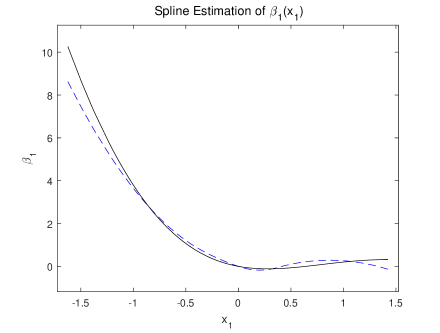
Reference

References

  • Cai et al. [2000] Cai, Z., Fan, J. and Yao, Q. (2000). Functional-coefficient regression models for nonlinear time series. J. Amer. Statist. Assoc. 95, 941–956.
  • Cai et al. [2008] Cai, Z. and Xu, X. (2008). Nonparametric quantile estimations for dynamic smooth coefficient models. J. Amer. Statist. Assoc. 103, 1595–1607.
  • Chiang et al. [2001] Chiang, C.-T., Rice, J. A. andWu, C. O. (2001). Smoothing spline estimation for varying coefficient models with repeatedly measured dependent variables. J. Amer. Statist. Assoc. 96, 605–619. MR1946428
  • Dahlhaus [1996a] Dahlhaus, R. (1996a). Asymptotic statistical inference for nonstationary processes with evolutionary spectra, in: Athens conference on applied probability and time series analysis, Springer. 145–259.
  • Dahlhaus [1996b] Dahlhaus, R. (1996b). On the kullback-leibler information divergence of locally stationary processes. Stochastic Process. Appl. 62, 139–168.
  • Dahlhaus [1997] Dahlhaus, R. (1997). Fitting time series models to nonstationary processes. Ann. Statist. 25, 1–37.
  • Dahlhaus [1999] Dahlhaus, R., Neumann, M. H., and Von Sachs. (1999). Nonlinear wavelet estimation of time-varying autoregressive processes. Bernoulli. 5, 873–906.
  • Dahlhaus [2006] Dahlhaus, R. and Rao, S. S. (2006). Statistical inference for time-varying arch processes. Ann. Statist. 34, 1075–1114.
  • De Boor [1978] De Boor, C. (1978). A Practical Guide to Splines. Springer-Verlag, New York.
  • Fan et al. [1998] Fan, J., Härdle, W. and Mammen, E. (1998). Direct estimation of low dimensional components in additive models. Ann. Statist. 26, 943–971.
  • Fan and Li [2001] Fan, J. and Li, R. (2001). Variable selection via nonconcave penalized likelihood and its oracle properties. J. Amer. Statist. Assoc. 96, 1348–1360.
  • Fan et al. [2002] Fan, J., Yao, Q., and Cai, Z. (2002). Adaptive varying-coefficient linear models. J. R. Stat. Soc. Ser. B. Stat. Methodol. 65, 57–80.
  • Fan and Zhang [1999] Fan, J. and Zhang, W. (1999). Statistical estimation in varying coefficient models. Ann. Statist. 27 1491–1518. MR1742497
  • Fryzlewicz et al. [2008] Fryzlewicz, P., Sapatinas, T. and Rao, S. S. (2008). Normalized least-squares estimation in time-varying arch models.Ann. Statist. 36, 742–786.
  • Fu [1998] Fu, W. (1998). Penalized regression: the bridge versus the lasso. J. Comput. Graph. Statist. 7, 397–416.
  • Hafner and Linton [2010] Hafner, C. M. and Linton, O. (2010). Efficient estimation of a multivariate multiplicative volatility model. J. Econometrics. 159, 55–73.
  • Hastie and Tibshirani [1990] Hastie, T. J. and Tibshirani, R. J. (1990). Generalized additive models. CRC Press.
  • Hastie and Tibshirani [1993] Hastie, T. J. and Tibshirani, R. J. (1993) Varying-coefficient models. J. Roy. Statist. Soc. B. 55 ,757–796. MR1229881
  • Hoover and Rice [1998] Hoover, D. R., Rice, J. A., Wu, C. O. and Yang, L.-P. (1998). Nonparametric smoothing estimates of time-varying coefficient models with longitudinal data. Biometrika. 85, 809–822. MR1666699
  • Horowitz et al. [2006] Horowitz, J., Klemelä, J. and Mammen, E. (2006). Optimal estimation in additive regression models. Bernoulli. 12, 271–298.
  • Huang [1998] Huang, J. Z. (1998). Projection estimation in multiple regression with application to functional anova models. Ann. Statist. 26 , 242–272.
  • Huang et al. [2002] Huang, J. Z., Wu, C. O. and Zhou, L. (2002). Varying-coefficient models and basis function approximations for the analysis of repeated measurements. Biometrika. 89, 111–128. MR1888349
  • Huang and Shen [2004] Huang, J. Z. and Shen, H. (2004). Functional coefficient regression models for nonlinear time series: A polynomial spline approach. Scand. J. Stat. 31, 515–534. MR2101537
  • Huang and Yang [2004] Huang, J. Z. and Yang, L. (2004). Identification of non-linear additive autoregressive models. J. R. Stat. Soc. Ser. B. Stat. Methodol. 66, 463–477.
  • Huang et al. [2004] Huang, J. Z.,Wu, C. O. and Zhou, L. (2004). Polynomial spline estimation and inference for varying coefficient models with longitudinal data. Statist. Sinica. 14 763–788. MR2087972
  • Huang et al. [2010] Huang, J., Horowitz, J. L. and Wei F. (2010) . Variable selection in nonparametric additive models. Ann. Statist. 38 , 2282–2313.
  • Kim et al. [1999] Kim, W., Linton, O. B., and Hengartner, N. W. (1999). A computationally efficient oracle estimator for additive nonparametric regression with bootstrap confidence intervals. J. Comput. Graph. Statist. 8, 278–297.
  • Linton and Nielsen [1995] Linton, O. and Nielsen, J. P. (1995). A kernel method of estimating structured nonparametric regression based on marginal integration. Biometrika. 93–100.
  • Linton [1997] Linton, O. (1997). Efficient estimation of additive nonparametric regression models. Biometrika. 84, 469–473.
  • Liu et al. [2013] Liu. R., Yang. L. and Härdle, W. K. (2013). Oraclly efficient two-step estimation of generalized aditive model. J. Amer. Statist. Assoc. 108, 619–631.
  • Koo and Linton [2012] Koo, B. and Linton, O. (2012). Semiparametric estimation of locally stationary diffusion models. J. Econometrics. 170, 210–233.
  • Mammen et al. [1999] Mammen, E., Linton, O. and Nielsen, J. (1999). The existence and asymptotic properties of a backfitting projection algorithm under weak conditions. Ann. Statist. 27, 1443–1490.
  • Priestley [1965] Priestley, M. B. (1965). Evolutionary spectra and non-stationary process. J. R. Stat. Soc. Ser. B. Stat. Methodol. 27, 204–237.
  • Stone [1982] Stone, C. J. (1982). Optimal global rates of convergence for nonparametric regression. Ann. Statist. 10, 1040–1053. MR0673642
  • Stone [1985] Stone, C. J. (1985). Additive regression and other nonparametric models. Ann. Statist. 13, 689–705.
  • Stone [1994] Stone, C. J. (1994). The use of polynomial splines and their tensor products in multivariate function estimation. Ann. Statist. 22, 118–171.
  • Tibshirani, R [1996] Tibshirani, R. (1996). Regression shrinkage and selection vis the Lasso. J. R. Stat. Soc. Ser. B. Stat. Methodol. 58, 267–288.
  • Tjøstheim and Auestad [1994] Tjøstheim, D. and Auestad, B. H. (1994). Nonparametric identification of nonlinear time series: projections.
  • Vogt [2012] Vogt, M. (2012). Nonparametric regression for locally stationary time series. Ann. Statist. 40, 2601–2633.
  • Wang and Yang [2007] Wang, L. and Yang, L. (2007). Spline-backfitted kernel smoothing of nonlinear additive autoregression model. Ann. Statist. 35, 2474–2503.
  • Wang and Yang [2009] Wang, J. and Yang, L. (2009). Efficient and fast spline-backfitted kernel smoothing of additive regression model. Ann. Inst. Statist. Math. 61, 663–690.
  • Wu et al. [1998] Wu, C. O., Chiang, C. T. and Hoover, D. R. (1998). Asymptotic confidence regions for kernel smoothing of a varying-coefficient model with longitudinal data. J. Amer. Statist. Assoc. 93 1388–1402. MR1666635
  • Xue and Yang [2006] Xue, L. and Yang, L.(2006). Estimation of semi-parametric additive coefficient model. J. Statist. Plann. Inference. 136, 2506–2534.
  • Xue and Yang [2009] Xue, Lan. (2009). Consistent variable selection in additive models. Statist. Sinica.19, 1281–1296.
  • Yang et al. [1999] Yang, L., Hardle, W. and Nielsen, J. (1999). Nonparametric autoregression with multiplicative volatility and additive mean. J. Time Series. Anal. 20, 579–604.
  • Yuan and Lin [2006] Yuan, M. and Lin, Y. (2006). Model selection and estimation in regression with grouped variables. J. R. Stat. Soc. Ser. B. Stat. Methodol. 68, 49–67.
  • Zhang [2013] Zhang, X. K., Park, B.U. and Wang, J. L. Time-Varying additive models for longitudinal data. J. Amer. Statist. Assoc. 108, 983–998.
  • Zhang and Wang [2015] Zhang, X. K, and Wang, J. L. (2013). Varying-coefficient additive models for functional data. Biometrika. 102, 15–32.
  • Zou [2006] Zou, H. (2006). The adaptive lasso and its oracle properties. J. Amer. Statist. Assoc. 101, 1418–1429.