CDVAE: Co-embedding Deep Variational Auto Encoder
for Conditional Variational Generation
Abstract
Problems such as predicting a new shading field () for an image () are ambiguous: many very distinct solutions are good. Representing this ambiguity requires building a conditional model of the prediction, conditioned on the image. Such a model is difficult to train, because we do not usually have training data containing many different shadings for the same image. As a result, we need different training examples to share data to produce good models. This presents a danger we call “code space collapse” — the training procedure produces a model that has a very good loss score, but which represents the conditional distribution poorly. We demonstrate an improved method for building conditional models by exploiting a metric constraint on training data that prevents code space collapse. We demonstrate our model on two example tasks using real data: image saturation adjustment, image relighting. We describe quantitative metrics to evaluate ambiguous generation results. Our results quantitatively and qualitatively outperform different strong baselines.
1 Introduction
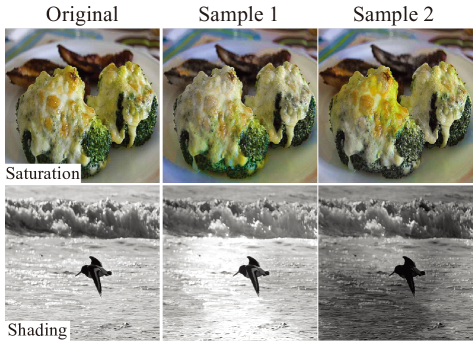
Many vision problems have ambiguous solutions. There are many motion fields consistent with an image [19, 25, 26]. Similarly, there are many shading fields consistent with the layout of an image (Figure 1); many good ways to colorize an image [3, 27, 29]; many possible ways to adjust the saturation of an image (Figure 1); many possible long term futures for an image frame [30]; and so on. For each of these problems, one must output a spatial field for an input image ; but is not uniquely determined by . Worse, has complex spatial structure (for example, saturation at a pixel is typically similar to the saturation at the next pixel, except over boundaries). It is natural to build a generative model of , conditioned on , and draw samples from that model. Towards this end, recent work has modified a strong generative model for images that uses latent variables, the variational auto-encoder (VAE) of [7], to produce a conditional VAE (CVAE) [19, 25, 26]. The very high dimension and complex spatial covariances of are managed by the underlying latent variable model in the CVAE.
However, building a good conditional model still poses some challenges. In most practical vision problems, the training dataset we can access is “scattered”, and the model is multimodal. Scattered training data consists of pairs of , but we never see multiple different values of for one particular . Practical vision models compute some intermediate representation (which we call the “code”), and predict from that intermediate representation and a random (or latent) variable . Write . The hope is that different choices of the random variable will produce different values of , and we can therefore predict the entire gamut of outputs (shading, motion field, saturation etc.). This implies that the method can represent a multimodal .
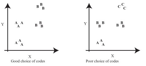
This setting presents a difficulty. To build a plausible conditional model, we must smooth. The model smooths by allowing examples with similar codes to “share” values. In turn, the choice of code is crucial, and a poor choice of code can result in a method that appears to work well, but does not. Figure 2 illustrates this point. The figure shows two possible choices of code for a particular dataset. In the good choice of code, is forced to use the random variable to produce distinct values of for similar , because similar result in similar codes. In the poor choice of code, similar can have different codes (viz. different codes A and B for similar in the right side of Figure 2) and vice versa. Then, can largely ignore the random variable, but simulates a multimodal process by producing very different for quite similar using the different . This means the network we have trained will (a) not be effective at making diverse predictions and (b) may change its prediction very significantly for a small change in , in a manner that is uncontrolled by the code. This is not desirable behavior.
We call the effect “code collapse”, because the network is encouraged to produce similar codes for different inputs. The result is a model with imperfect diversity and generalization, but good loss on scattered training data. The absence of variance, in what should be a diverse pool of output predictions, is a strong diagnostic indicator of code collapse. We exploit this indicator and show that our baselines, particularly the CVAE, generate low variance and therefore suffer from code collapse (Section 5.2, Figure 5).
The key problem, resulting in code collapse, is that the current training procedures have no term to force a good choice of codes. For example, VAE loss requires the code distribution to look like a standard normal distribution. This loss does not force it to preserve the similarity, dissimilar input images can be closer and similar inputs further apart in the code space. Recent work shows that better generative models are obtained by conditioning on text-embeddings [15] or pre-trained features from visual recognition network [12]. This suggests that using an embedding with some structure is better than conditioning on raw pixels (with high-capacity networks).
In our approach, instead of using a fixed embedding as input, we use raw pixels but guide the codes (or intermediate representation) with a metric constraint. Our metric term encourages codes for distinct to be different and codes for similar to be similar. This prevents code collapse. To ensure that will vary for similar , we use a Mixture Density Network (MDN) [2]. MDN explicitly models a multimodal conditional distribution. We call our model CDVAE (Co-Embedding Deep Variational Auto Encoder).
We apply CDVAE to two novel (from the point of view of automated editing) problems: (a) Photo Relighting,
(b) Image Resaturation (Section 4). In relighting (or reshading), we decompose the image into shading and albedo, then produce a new shading
field consistent with the albedo field. In resaturation, we produce a new saturation field and
apply it to the image. In each case, the resulting image should look “natural” – like
a real image, but differently illuminated (reshading) or with differently color saturated objects
(resaturation). In all cases, our model outperforms strong baselines
(including the CVAE).
Contributions:
- •
- •
- •
- •
2 Related Work
Generating a spatial field with complex spatial structure from an image is an established problem. Important application examples, where the prediction is naturally ambiguous, include colorization [4, 9, 29], style transfer [5], temporal transformations prediction [30], predicting motion fields [19, 25, 26], and predicting future frames [24]. This is usually treated as a regression problem; current state of the art methods use deep networks to learn features. However, predicting the expected value of a conditional distribution, through regression, works poorly, because the expected value of a multimodal distribution may have low probability. While one might temper the distribution (eg [29]), the ideal is to obtain multiple different solutions.
One strategy is to draw samples from a generative model. Generative models of images present problems of dimension; these can be addressed with latent variable models, leading to the variational autoencoder (VAE) of [7]. As the topic attracts jargon, we review the standard VAE briefly here. This approach learns an encoder that maps data into a continuous latent variable (the codes), and a decoder that maps to an image . Learning ensures that (a) and are close; (b) if is close to , then is close to ; and (c) is distributed like a standard normal random variable. Images can then be generated by sampling a standard normal distribution to get , and forming . This is a latent variable model, modelling as . is represented by the decoder, we use an auxiliary distribution for , where is now the encoder. Learning is by maximizing a lower-bound on log-likelihood (Equation 1)
| (1) |
where are the parameters of encoder and decoder networks of the VAE.
Current generative models are reliable in simple domains (handwritten digits [7, 18]; faces [7, 8, 16]; and CIFAR images [6]) but less so for general images. Improvements are available using multiple layers of latent variables (a DVAE) [16]. Models can be trained with adversarial loss [14]. However, these deep models are still hard to train. The ladder VAE imposes both top-down and bottom up variational distributions for more efficient training [20].
The generative model needs to be conditioned on an image, and needs to be multimodal. Tang et al. give a multimodal conditional model [21], but the conditioning variables are binary. A conditional variational autoencoder (CVAE) [19] conditions the decoder model on a continuous representation produced by a network applied to . This approach has been demonstrated on motion prediction problems [25, 30].
We use the mixture density network (MDN) in our models to capture the underlying multimodal distribution [2]. MDN predicts the parameters of a mixture of gaussians from real-valued input features. MDNs have been successfully applied to articulatory-acoustic inversion mapping [17, 22] and speech synthesis [28].
3 Method
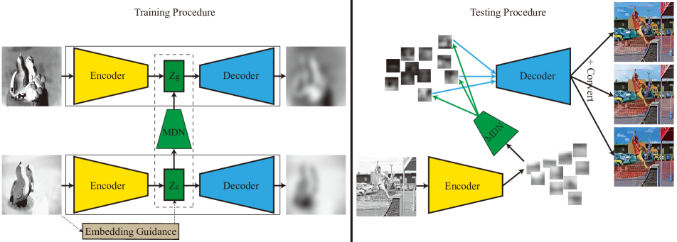
Our CDVAE consists of two deep variational auto encoders (DVAE) [16] and a mixture density network (MDN) [2]. An overview of the CDVAE model is shown in Figure 3.
Our architecture is, we use two DVAEs to embed the conditioning image (or from Section 1) and the generated image (or from Section 1) into two low-dimensional latent variables (or code spaces) and . The generated image corresponds to output spatial field viz. saturation or shading etc. and the conditioning image is the input image viz. intensity or albedo etc. Next, we regularize the latent variables with embedding guidance (or metric constraints) such that the similarity in input space is maintained (Section 3.2). Since our problem is ambiguous, the conditional distribution between and is multimodal. MDN allows us to fit a multimodal gaussian mixture model (GMM) between the conditioning code and the generated code (Section 3.1). At test time, we sample from this multimodal GMM () and use the decoder of the generated image DVAE () to predict different shading, saturation for a single input image.
In Figure 3, we simplify and show a single layer of latent variables. In practice, our DVAE utilizes multiple layers of gaussian latent variables. This hierarchical variational auto encoder architecture captures complex structure in the data, and provides good practical performance.
We jointly train the two DVAEs and the MDN, allowing them to adapt and mutually benefit each other. Joint training also enables CDVAE to model a joint probability distribution of and , instead of a conditional probability distribution (viz. like a CVAE). The joint probability model allows for more smoothing between data points. In CDVAE, we optimize the joint probability model during training (Refer Equation 25). At test time, we remove the decoder for the conditioning layer and the encoder for the generated layer. This converts the joint model of CDVAE into a conditional model . We can then sample this conditional model to generate diverse outputs. Similar to VAE probability model, we write the joint probability by marginalizing over the joint distribution
| (2) |
In Section 3.1, we derive the loss terms corresponding to this joint probability model of CDVAE.
3.1 CDVAE Loss
In CDVAE, we use two multi-layer variational auto encoders (DVAE), one for and one for . Additionally, we have an MDN that models the relationship between the embeddings and . The loss function corresponding to the CDVAE joint model is a combination of the two DVAE models and the conditional probability model of MDN. In Equations 1 and 25, assume it is possible to encode without seeing , then we can use the auxiliary sampling distribution for our CDVAE. If in Equation 25, we can separate out the product terms of joint probability model. Taking negative log-likelihood, we obtain separate additive loss terms for each DVAE. Write for the loss function of a DVAE with weights (or parameters) , which has the standard form of a VAE loss (Equation 1). Write the loss of the DVAE for the generated image as (similarly for ). Write loss for the MDN as . We can then derive the loss function for CDVAE (Equation 3),
| (3) |
Our MDN estimates the conditional probability model . For each input code , our MDN estimates the parameters of a component gaussian mixture distribution with mixture coefficients , means and fixed diagonal covariance . The loss is obtained by taking the negative log-likelihood of this conditional distribution,
| (4) |
We use an inference method [20] that co-relates the latent variables of the encoder and the decoder. This speeds up the training. Refer to the supplementary materials for the detailed derivations.
3.2 Embedding Guidance: Preventing code collapse
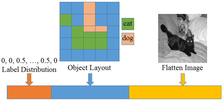
Vanilla DVAEs have difficulty in learning a code space which encodes the complex spatial structure of the output. The code space learned by a DVAE appears to be underdetermined, especially for large and complex datasets. This is a common failure mode of VAEs. For our conditional models, it is desirable that codes for “similar” inputs are nearby, and codes for “very different” inputs are further apart. This discourages the method from grouping together very different inputs. It also prevents similar images from having different codes, and therefore avoids incorrect smoothing of the model (See Figure 2). We guide the codes (at multiple layers) to be similar to a pre-computed embedding. Our pre-computed embedding is such that it preserves the similarity observed in input domain. Refer to Figure 4 and supplementary material for the details of our pre-computed embedding. Write for the pre-computed embedding and for the gaussian latent variables of the network. We use the L2-norm between and as a loss term
| (5) |
Write for the final loss function with the additional regularization in the form of embedding guidance
| (6) |
We use a large value of when training starts and gradually reduce it during the training process.
3.3 Post Processing
Current deep generative models only handle small images, for our case , and they generate results without high spatial frequencies. We post process generated images for viewing at high resolution (not used in any quantitative evaluation). Our post processing upsamples results to a resolution of , with more details. We aggressively upsample the generated fields with the approach in [10], which preserves edges during upsampling. In particular, the method represents a high resolution field by a weight and an orientation value at each sample point; these parameters control a basis function placed at each sample, and the field at any test point is a sum of the values of the basis functions at that point. The sum of basis functions includes only those basis functions in the same image segment. Write for the high resolution field produced by interpolating a weight vector and a vector of orientations , assuming a segment mask obtained from the high resolution grey level image. Write for a low resolution field produced by the decoder, and for a process that smooths and downsamples. We solve
for , , regularizing with the magnitude of . This produces a high resolution field that (a) is compatible with the high resolution edges of the grey level image (unlike the learned upsampling in common use) and (b) produces the decoder sample when smoothed.
For relighting and saturation adjustment tasks, we polish images for display by using detail maps to recover fine scale details. The detail map is calculated by taking the conditioning image and subtracting the output produced by the conditioning image decoder with the code . This captures the high frequency details lost during the neural network process. We get our result as
| (7) |
4 Applications
We apply our methods to two different ambiguous tasks, each of which admits both quantitative and qualitative evaluations.

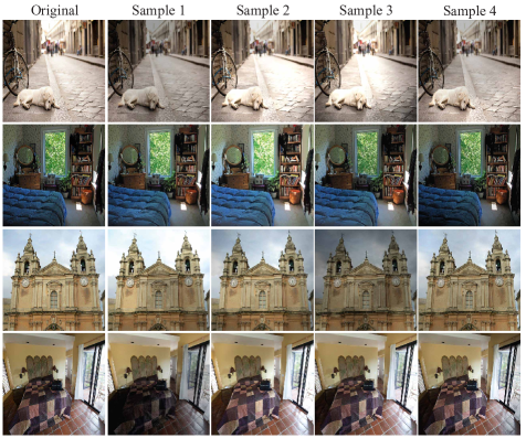
Photo Relighting (or Reshading): In this application, we predict new shading fields for images which are consistent with a relit version of the scene. We decompose the image into albedo (the conditioning image ), and shading (the generated image ). In real images, shading is quite strongly conditioned by albedo because the albedo image contains semantic information such as the scene categories, object layout and potential light sources. A scene can be lighted in multiple ways, so relighting is a multimodal problem. We use the MS-COCO dataset for relighting (Section 5.1).
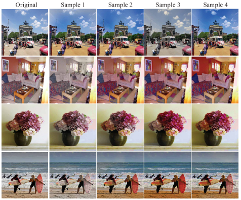
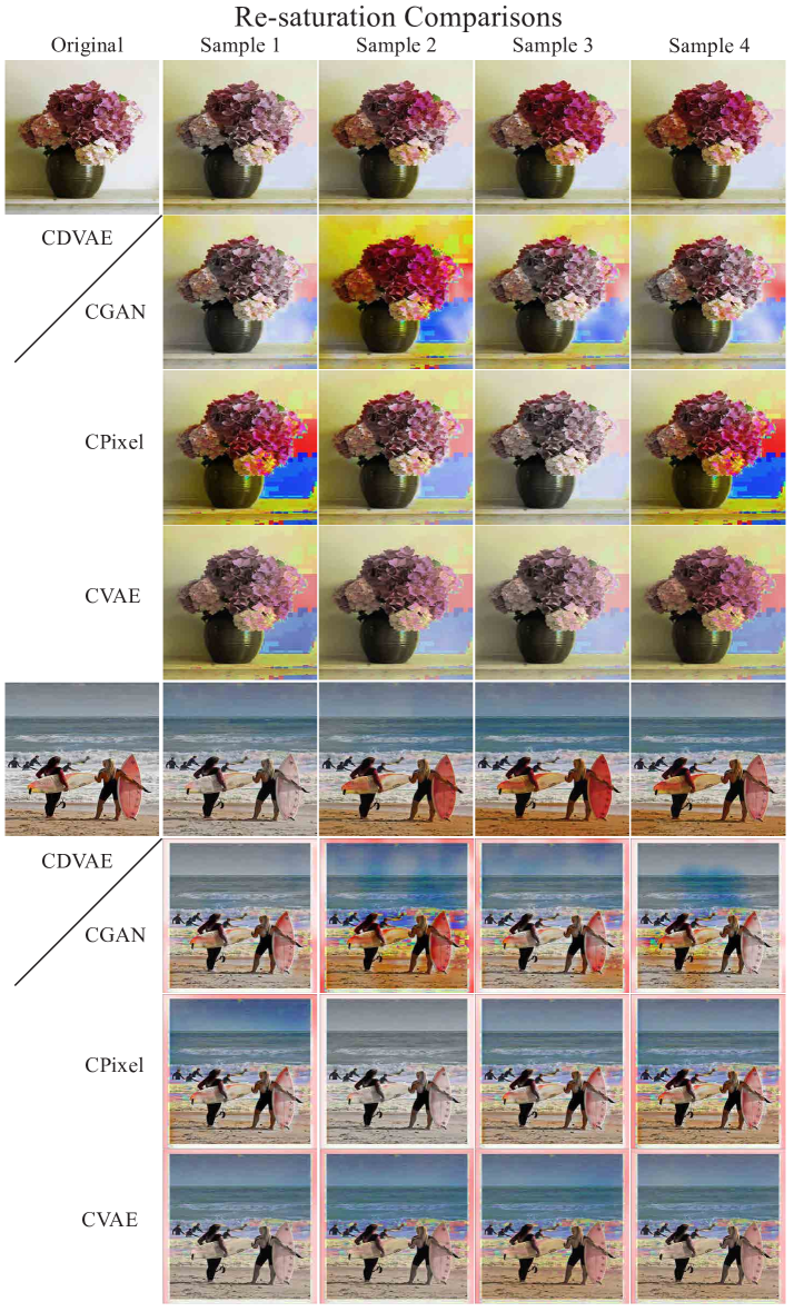
Image Resaturation: Here, we predict new saturation fields for color images, i.e. we modify color saturation for some or all objects in the image. We transform the input RGB color image into HSV color space, and use the value channel as our conditioning image and the saturation channel as our generated image. We use CDVAE to generate new saturation fields consistent with the input value image. Combining the new saturation fields with H and V channels leads to new versions of an image, with edited saturation. See the grilled cheese on the broccoli in Figure 1 which demonstrates that we obtain natural edits. Again, we use the MS-COCO dataset for this application (Section 5.1).
5 Results
To evaluate the effectiveness of our method, we compare with recent strong methods (Section 5.3). We also evaluate different variants of our method. We perform quantitative and qualitative comparison on applications of photo relighting, image resaturation. Quantitative results (Section 5.2, Figure 5) are computed on the network output, without any post processing. Images shown for qualitative evaluation of resaturation and reshading (Section 5.4, Figures 1, 6, 8 and 7) are post processed using the steps described in Section 3.3. We downsample all the input images to dimensions, and all neural network operations before post processing are performed on this image size. After our CDVAE model generates samples, our post processing upsamples it to a resolution of .
5.1 Datasets
MS-COCO: We use MS-COCO dataset for our both the tasks, photo relighting and image resaturation. It is a wild dataset (unlike the structured face data commonly used by generative models), and has complex spatial structure. Typically, such data is challenging for VAE-based methods. We use train2014 (80K images) for model training, and sample 6400 images from val2014 (40K images) for testing. For photo relighting, intrinsic image decomposition method from [1] is used to obtain albedo and shading images. For image resaturation, we transform the image from RGB space to HSV space.
5.2 Quantitative Metrics and Evaluation
Error-of-Best to ground truth: We follow the motion prediction work [25] to use error-of-best to ground truth as an evaluation metric. We draw 100 samples for each conditional model and calculate the minimum per pixel error to ground truth fields. A better model will produce smaller values, because it should produce some samples closer to the ground truth.
Variance: A key goal of our paper is to generate diverse solutions. However, no current evaluation regime can tell whether a pool of diverse solutions is right. We opt for the strictly weaker proxy of measuring variance in the pool, on the reasonable assumption that diverse predictions for our problems must have high variance. Thus, procedures that produce low variance predictions are clearly unacceptable. Clearly, it is not enough just to produce variance – we want the pool to contain appealing diverse predictions. To assess this, we rely on qualitative evaluations (Figures 6, 7, 8). The supplementary materials contain many additional qualitative results.
To compute variance, we obtain the values for 16 () equally spaced grid (since distant pixels are de-correlated to some extent) of pixels in our prediction. We collect these values across 100 samples, and compute the variance at each grid point across samples. We report this average variance vs. minimum error (See Figure 5). In particular, a method with more diverse output predictions should result in higher variances and one of them should also be close to the ground-truth (therefore, low minimum error). Specifically, we need to be in the bottom-right part of Figure 5, which our CDVAE achieves.
Therefore, our CDVAE model creates results with desirable properties: lower error-of-best to ground truth and large variance. Our CDVAE model produces better results with more gaussian kernels (CDVAE12 vs. CDVAE4) and performance drops (higher minimum error and low variance) when no embedding guidance is used (CDVAE4 noemb).
5.3 Baseline Methods
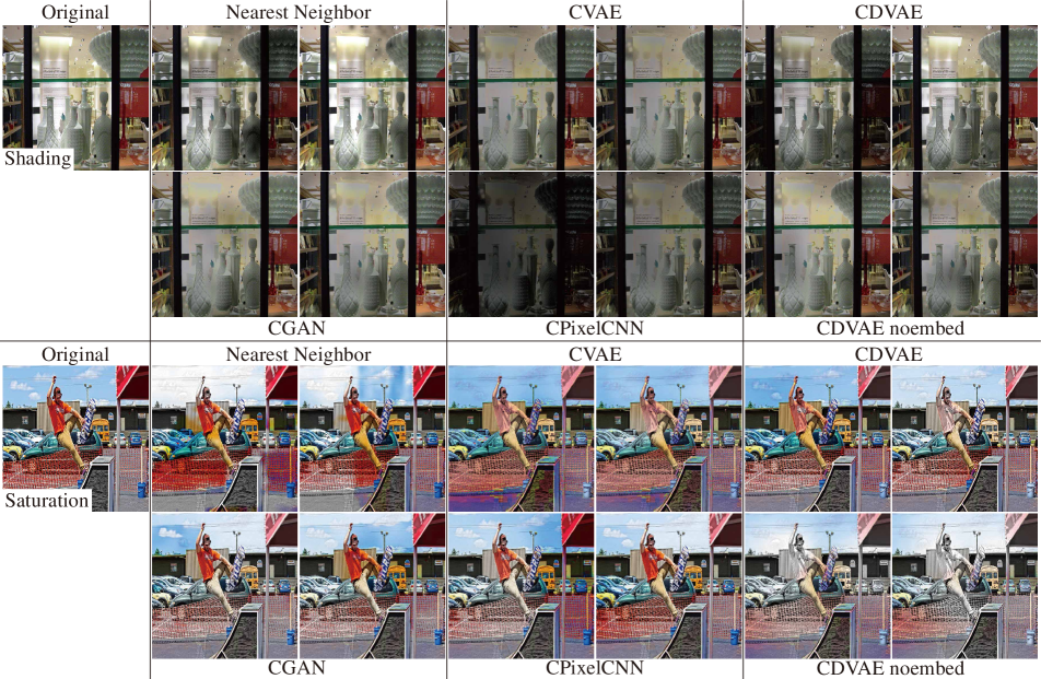
Nearest neighbor (NN): We perform top nearest neighbor (NN) search in space, and return the corresponding as multiple outputs. Gaussian smoothing is applied to returned to remove inconsistent high frequency signal. Since our training data does not have explicit one-to-many correspondences, NN is a natural strong baseline. It is a non-parametric method to model multimodal distribution by borrowing output spatial fields (we also smooth these) from nearby input images.
Conditional variational autoencoder: We implement a CVAE similar to [25]. We cannot use [25] since their architecture is specific to prediction of coarse motion trajectories. Our decoder is modelled on the DCGAN architecture of Radford et al. [14] with 5 deconvolution layers, and we use codes of dimension (to be consistent with CDVAE). Our image tower and encoder tower use 5 convolutional layers (mirror image of the decoder). We use the same strategy as [25], i.e. we spatially replicate code from encoder and multiply it to the output of image tower. The decoder takes as input the result of this. We train our CVAE with the standard pixel-wise L2 loss on output and KL-divergence loss on the code space. At test time, codes are randomly sampled from the normal distribution.
Conditional GAN: CGAN [11] is another conditional image generation model. It uses a regularized code (drawn from a uniform distribution) along with a fixed embedding of the conditioning image as input. We observe that CGAN achieves higher minimum error (or error-of-best) and lower variance as compared to CDVAE (See Figure 5). Therefore, we generate better (lower minimum error) and more diverse (higher variance) predictions that CGAN. These metrics are explained in detail in Section 5.2.
Conditional PixelCNN (CPixel): Conditional PixelCNN [23] uses masked and gated convolutions (sigmoid and tanh activations layers multiplied). The receptive field of masked convolutions mimics the causal dependency and gated convolutions approximate the behavior of LSTM gates in recurrent architectures. Therefore, PixelCNN (CPixel) feasibly approximates the compute intensive recurrent architectures [6] for image generation. However, their receptive field grows linearly and handling long-scale effects is difficult. Our results are qualitatively better than PixelCNN, we believe our DVAE with fully-connected layers is better at capturing the global structure given the coarse resolution used. Note, our CDVAE has lower minimum error than PixelCNN (Figure 5).
5.4 Qualitative Evaluation
In addition to outperforming baselines on quantitative results, our method generates better qualitative results. Samples from our jointly trained conditional model smooth information across “similar” images, allowing us to produce aligned, semantically sensible and reasonable diverse predictions. Our qualitative comparisons with other methods for the two tasks is shown in Figure 6. In both examples, we generate plausible and diverse relighted scenes and resaturated image.
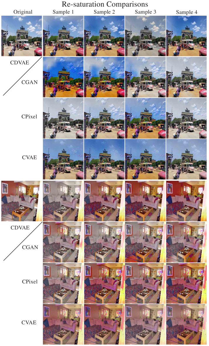
Image Resaturation: More results for image resaturation with our CDVAE (12 gaussian kernels) and embedding guidance are shown in Figure 7. For each input image, we draw four samples for saturation fields from our conditional model. The diverse saturation adjustment results show that our model learns multimodal saturation distributions effectively. Our automatic saturation adjustment creates appealing photos. We demonstrate artistic stylization/editing by using our automated method.
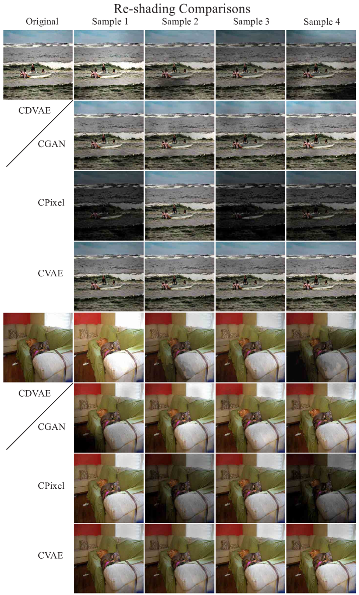
Photo Relighting: In Figure 8, we show additional photo relighting results from our method. For each input image, we again draw four samples from the distribution. The photo relighting results show that our CDVAE model learns the light source distributions as well as important objects. Our model creates light fields coming from reasonable light sources and the lighting looks natural, especially on important objects.
6 Discussion
Our CDVAE generates good results qualitatively and quantitatively. However, there are still some limitations. Some of them are due to the limitations of VAE based generative models. For example, variational auto-encoders and its variants oversmooth their outputs, which leads to loss of spatial structure. Our multilayer gaussian latent variable architecture can capture more complex structures, but we do miss out on the finer details compared to ground truth. Second, our model – like all current generative models – is applied to low resolution images, meaning that much of the structural and semantic information important to obtaining good results is lost. Last, our model has no spatial hierarchy. Coarse to fine multiscale hierarchy on both generative side and conditional side would likely enable us to produce results with more details.
7 Conclusion
We described an approach that simplifies building conditional models by building a joint model. Our joint model yields a conditional model that can be easily sampled. This allows us to train on scattered data using a joint model. We have demonstrated our approach on the task of generating photo-realistic relighted and resaturated images. We propose a metric regularization of code space which prevents code collapse. In future, this regularization can be investigated in the context of other generative models.
8 Appendix
8.1 Architecture Details
Our CDVAE has a different architecture compared to a CVAE. The detailed architecture of our CDVAE is in Table 1. Write for the input layer and for the output layer, stands for a fully connected layer, is the mean of the gaussian distribution of the code space, and is the variance of the gaussian distribution of the code space. is the process of sampling the gaussian distribution with and . is sampled from and . We use regularization (or weight decay) for the parameters for MDN model. The learning rate is set to and we use the ADAM optimizer. We initially set the reconstruction cost high, LPP embedding guidance cost high, and MDN cost low. We keep this setting and train for 100 epochs. For the next 200 epochs, we gradually decrease the embedding cost, and increase the MDN cost. Finally, we keep the relative cost fixed and train another 200 epochs.
| Layers | Conditional DVAE | ( is GMM num) | Generative DVAE | ||||||||
|---|---|---|---|---|---|---|---|---|---|---|---|
| (None, 1024) | (None, 1024) | ||||||||||
| (1024, 512) | (1024, 512) | ||||||||||
| Leaky Rectify | Leaky Rectify | ||||||||||
| (512, 512) | (512, 512) | ||||||||||
| Leaky Rectify | Leaky Rectify | ||||||||||
| (512, 64) | (512, 64) | (512, 64) | (512, 64) | ||||||||
| Identity | SoftPlus | Identity | SoftPlus | ||||||||
| (None, 64) | (None, 64) | (None, 64) | (None, 64) | ||||||||
| (None, 64) | (None, 64) | ||||||||||
| (64, 256) | (64, 256) | ||||||||||
| Leaky Rectify | Leaky Rectify | ||||||||||
| (256, 256) | (256, 256) | ||||||||||
| Leaky Rectify | Leaky Rectify | ||||||||||
| (256, 32) | (256, 32) | (256, 32) | (256, 32) | ||||||||
| Identity | SoftPlus | Identity | SoftPlus | ||||||||
| (None, 32) | (None, 32) | (None, 32) | (None, 32) | ||||||||
| (None, 32) |
|
(None, 32) | |||||||||
| (32, 256) | (32, 256) | ||||||||||
| Leaky Rectify | Leaky Rectify | ||||||||||
| (256, 256) | (256, 256) | ||||||||||
| Leaky Rectify | Leaky Rectify | ||||||||||
| (256, 64) | (256, 64) | (256, 64) | (256, 64) | ||||||||
| Identity | SoftPlus | Identity | SoftPlus | ||||||||
| (None, 64) | (None, 64) | (None, 64) | (None, 64) | ||||||||
| (None, 64) | (None, 64) | ||||||||||
| (64, 512) | (64, 512) | ||||||||||
| Leaky Rectify | Leaky Rectify | ||||||||||
| (512, 512) | (512, 512) | ||||||||||
| Leaky Rectify | Leaky Rectify | ||||||||||
| (512,1024) | (512,1024) | (512,1024) | (512,1024) | ||||||||
| Identity | SoftPlus | Identity | SoftPlus | ||||||||
| (None, 1024) | (None, 1024) | (None, 1024) | (None, 1024) | ||||||||
| (None, 1024) | (None, 1024) | ||||||||||
8.2 DVAE
The difference between DVAE [16] and VAE [7] is multiple layers of gaussian latent variables. DVAE for (same for ) consists of layers of latent variables. To generate a sample from the model, we begin at the top-most layer () by drawing from a Gaussian distribution to get .
| (8) |
The mean and variance for the Gaussian distributions at any lower layer is formed by a non-linear transformation of the sample from above layer.
| (9) |
| (10) |
where represents multi-layer perceptrons. We descend through the hierarchy by one hot vector sample process.
| (11) |
where are mutually independent Gaussian variables. is generated by sampling from the Gaussian distribution at the lowest layer.
| (12) |
The joint probability distribution of this model is formulated as
| (13) |
where . Other details of the DVAE model are similar to VAE.
8.2.1 Inference
DVAE with several layers of dependent stochastic variables are difficult to train which limits the improvements obtained using these highly expressive models. LVAE [20] recursively corrects the generative distribution by a data dependent approximate likelihood in a process resembling the recent Ladder Network. It utilizes a deeper more distributed hierarchy of latent variables and captures more complex structures. We follow this work and for , write and for the mean and variance on the ’s level of generative side, write and for the mean and variance on the ’s level of inference side.
This changes the notation in the previous part on the generative side.
| (14) |
| (15) |
| (16) |
| (17) |
On the inference side, the notation also changes.
| (18) |
| (19) |
| (20) |
During inference, first a deterministic upward pass computes the approximate distribution and . This is followed by a stochastic downward pass recursively computing both the approximate posterior and generative distributions.
| (21) |
| (22) |
| (23) |
| (24) |
where and .
8.3 Joint Models
First, we prove that if the joint probability is independent, we will get two separate DVAEs. Then, we prove the derivations for joint model with non-independent joint probability.
8.3.1 Separate DVAEs
From Section 3 in the paper, the joint probability in CDVAE model is
| (25) |
If and are independent, so , and Equation 25 can be transformed
| (26) |
where is DVAE model for and is DVAE model for .
8.3.2 Joint Model Derivation
From Section 2 in the paper, we have objective function for VAE as
| (27) |
where . Applying the same derivations, the objective function for our CDVAE model can be written as
|
|
(28) |
where . Assume it is possible to encode without seeing , then the variational distribution applies. It is also possible to decode without seeing , so we have . With these formulas, Equation 28 can be transformed
| (29) |
where and . The joint distribution can be written as , so we have the following equations for the second part.
| (30) |
In our CDVAE model, we have and because and are Gaussian distributions. Our CDVAE objective function turns into
|
|
(31) |
8.4 Embedding Influence
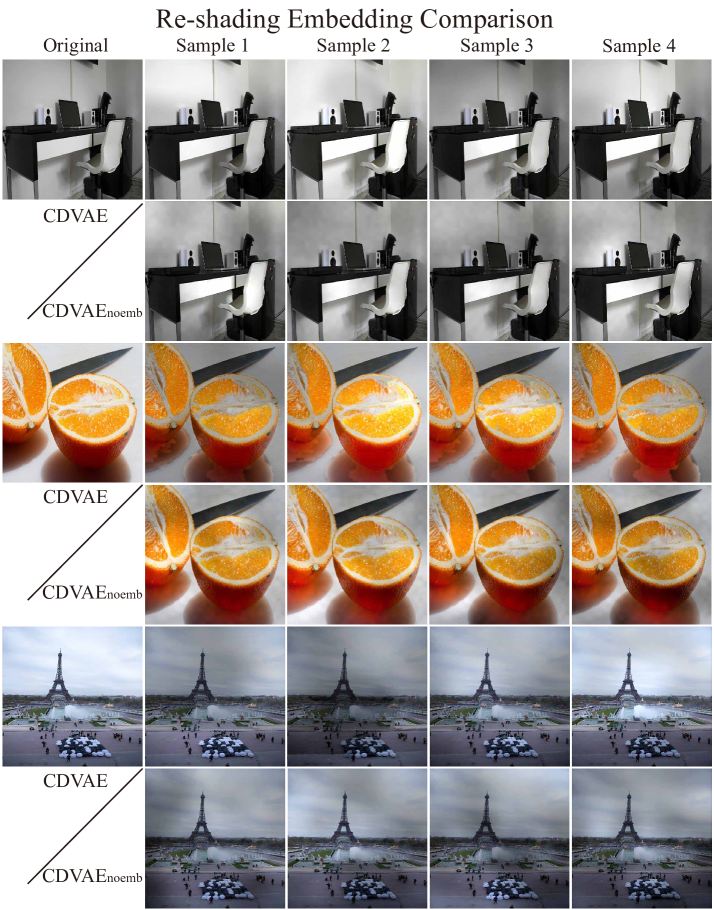
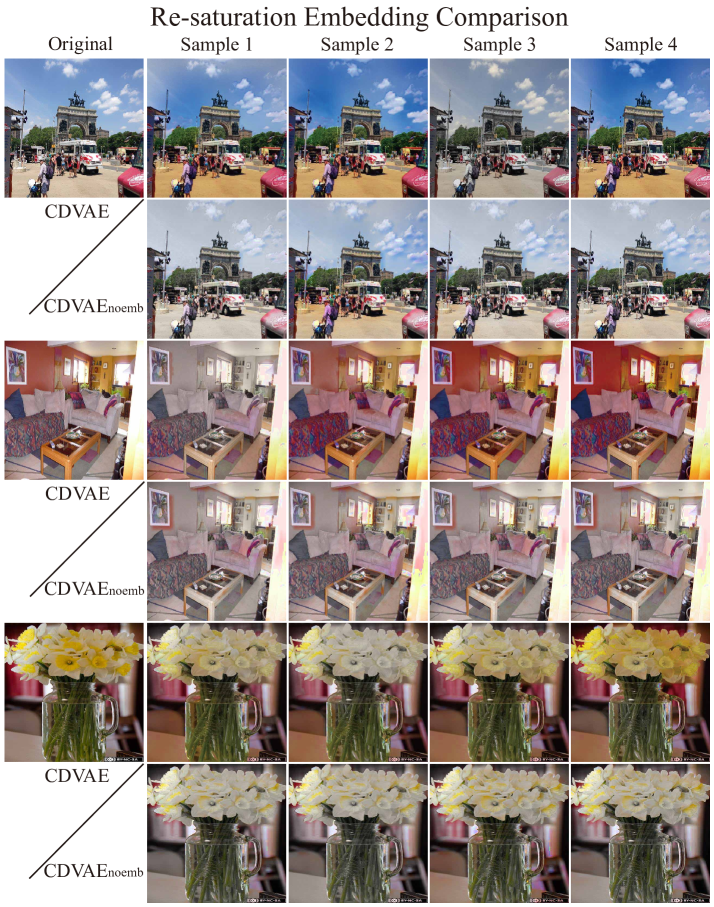
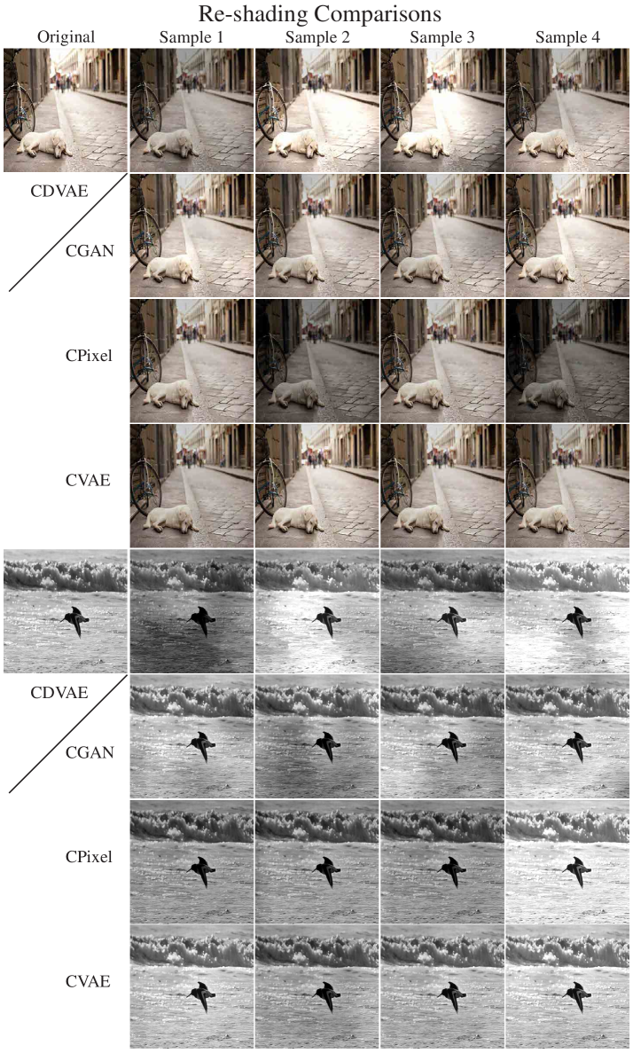
We compare the results with embedding guidance and without embedding guidance. The comparisons for re-shading can be found in Figures 9. The re-shading results without embedding guidance tend to have less variety, more flaws and artifacts. The comparisons for re-saturation can be found in Figures 10. The re-saturation results without embedding guidance tend to have limited variety and produce less vivid results.
8.5 Quantitative Results
The detailed quantitative evaluation results for photo relighting are in Table 2 and image resaturation are in Table 3. The tables contain best error to ground-truth with different sample numbers. As the sample number increases, the error drops fast at beginning, and then becomes stable. Our CDVAEs are consistently better than other methods. The second parts of both tables are average variances across 100 samples. We only report the final variance, since it almost does not change with the sample number. The variance we report comes from 100 samples.
| Best Error to Ground Truth | Variance | |||||
| Sample# 3 | Sample# 10 | Sample# 30 | Sample# 60 | Sample# 100 | Sample# | |
| NN | 3.04 | 2.30 | 1.93 | 1.76 | 1.66 | 1.61 |
| CVAE | 2.07 | 1.83 | 1.68 | 1.60 | 1.56 | 0.19 |
| CGAN | 3.07 | 2.49 | 2.16 | 2.02 | 1.94 | 1.19 |
| CPixel | 3.06 | 2.32 | 1.91 | 1.74 | 1.59 | 1.92 |
| 2.78 | 2.19 | 1.82 | 1.66 | 1.57 | 1.39 | |
| CDVAE4 | 2.44 | 1.66 | 1.33 | 1.20 | 1.11 | 1.77 |
| CDVAE12 | 2.49 | 1.69 | 1.33 | 1.20 | 1.12 | 1.74 |
| Best Error to Ground Truth | Variance | |||||
| Sample# 3 | Sample# 10 | Sample# 30 | Sample# 60 | Sample# 100 | Sample# | |
| NN | 10.12 | 8.40 | 7.09 | 6.52 | 6.20 | 4.58 |
| CVAE | 6.73 | 5.59 | 4.93 | 4.53 | 4.25 | 1.20 |
| CGAN | 8.06 | 6.20 | 5.37 | 5.03 | 4.83 | 4.79 |
| CPixel | 7.94 | 6.43 | 5.94 | 5.51 | 5.29 | 4.34 |
| 7.08 | 5.74 | 4.95 | 4.57 | 4.32 | 1.53 | |
| MDN4 | 6.62 | 5.11 | 4.37 | 4.05 | 3.86 | 3.48 |
| MDN12 | 6.40 | 5.04 | 4.33 | 4.02 | 3.82 | 3.55 |
8.6 Qualitative Results
We include more qualitative results and comparisons in this section. Photo relighting results and comparisons can be found in Figure 11, 12. Photo relighting results with CGAN tend to have less variety and be less reasonable; results with CPixel tend to be extreme and random, and they also have less spatial structures; results with CVAE suffers from mode collapsion and have limited variety. Image re-saturation results and comparisons can be found in Figure 13, 14. Image re-saturation results with CGAN tend to ignore the image content and like random, and creates various of artifacts; results with CPixel tend to be extreme, and either like random or go into mode collapsion; results with CVAE have limited variety and creates more artifacts.
References
- [1] S. Bell, K. Bala, and N. Snavely. Intrinsic images in the wild. ACM Trans. Graph., 33(4):159:1–159:12, July 2014.
- [2] C. M. Bishop. Mixture density networks. 1994.
- [3] A. Deshpande, J. Lu, M. Yeh, and D. A. Forsyth. Learning diverse image colorization. CoRR, abs/1612.01958, 2016.
- [4] A. Deshpande, J. Rock, and D. Forsyth. Learning large-scale automatic image colorization. In Proceedings of the IEEE International Conference on Computer Vision, pages 567–575, 2015.
- [5] L. A. Gatys, A. S. Ecker, and M. Bethge. Image style transfer using convolutional neural networks. In Proceedings of the IEEE Conference on Computer Vision and Pattern Recognition, Jun 2016.
- [6] K. Gregor, I. Danihelka, A. Graves, D. J. Rezende, and D. Wierstra. DRAW: A recurrent neural network for image generation. In Proceedings of the 32nd International Conference on Machine Learning, ICML 2015, Lille, France, 6-11 July 2015, pages 1462–1471, 2015.
- [7] D. P. Kingma and M. Welling. Auto-encoding variational bayes. International Conference on Learning Representations (ICLR), 2014.
- [8] T. D. Kulkarni, W. F. Whitney, P. Kohli, and J. Tenenbaum. Deep convolutional inverse graphics network. In Advances in Neural Information Processing Systems, pages 2539–2547, 2015.
- [9] G. Larsson, M. Maire, and G. Shakhnarovich. Learning representations for automatic colorization. In European Conference on Computer Vision (ECCV), 2016.
- [10] J. Lu and D. Forsyth. Sparse depth super resolution. In 2015 IEEE Conference on Computer Vision and Pattern Recognition (CVPR), pages 2245–2253. IEEE, 2015.
- [11] M. Mirza and S. Osindero. Conditional generative adversarial nets. arXiv preprint arXiv:1411.1784, 2014.
- [12] A. Nguyen, J. Yosinski, Y. Bengio, A. Dosovitskiy, and J. Clune. Plug & play generative networks: Conditional iterative generation of images in latent space. CVPR, 2017.
- [13] X. Niyogi. Locality preserving projections. 2004.
- [14] A. Radford, L. Metz, and S. Chintala. Unsupervised representation learning with deep convolutional generative adversarial networks. arXiv preprint arXiv:1511.06434, 2015.
- [15] S. E. Reed, Z. Akata, S. Mohan, S. Tenka, B. Schiele, and H. Lee. Learning what and where to draw. In Advances in Neural Information Processing Systems 29, pages 217–225. 2016.
- [16] D. J. Rezende, S. Mohamed, and D. Wierstra. Stochastic backpropagation and approximate inference in deep generative models. ICML’14, pages II–1278–II–1286. JMLR.org, 2014.
- [17] K. Richmond. Trajectory mixture density networks with multiple mixtures for acoustic-articulatory inversion. In International Conference on Nonlinear Speech Processing, pages 263–272. Springer, 2007.
- [18] T. Salimans et al. Markov chain monte carlo and variational inference: Bridging the gap.
- [19] K. Sohn, H. Lee, and X. Yan. Learning structured output representation using deep conditional generative models. In Advances in Neural Information Processing Systems, pages 3483–3491, 2015.
- [20] C. K. Sønderby, T. Raiko, L. Maaløe, S. K. Sønderby, and O. Winther. Ladder variational autoencoders. In Advances in Neural Information Processing Systems 29: Annual Conference on Neural Information Processing Systems 2016, December 5-10, 2016, Barcelona, Spain, pages 3738–3746, 2016.
- [21] Y. Tang and R. R. Salakhutdinov. Learning stochastic feedforward neural networks. In Advances in Neural Information Processing Systems, pages 530–538, 2013.
- [22] B. Uria, I. Murray, S. Renals, and K. Richmond. Deep architectures for articulatory inversion. In Proceedings of Interspeech, pages 866–870. Curran Associates, 2012.
- [23] A. van den Oord, N. Kalchbrenner, O. Vinyals, L. Espeholt, A. Graves, and K. Kavukcuoglu. Conditional image generation with pixelcnn decoders. CoRR, abs/1606.05328, 2016.
- [24] C. Vondrick, H. Pirsiavash, and A. Torralba. Anticipating visual representations from unlabeled video. In 2016 IEEE Conference on Computer Vision and Pattern Recognition, CVPR 2016, Las Vegas, NV, USA, June 27-30, 2016, pages 98–106, 2016.
- [25] J. Walker, C. Doersch, A. Gupta, and M. Hebert. An uncertain future: Forecasting from static images using variational autoencoders. In European Conference on Computer Vision, pages 835–851. Springer, 2016.
- [26] T. Xue, J. Wu, K. Bouman, and B. Freeman. Visual dynamics: Probabilistic future frame synthesis via cross convolutional networks. In Advances in Neural Information Processing Systems 29, pages 91–99. 2016.
- [27] W. Z. Yun Cao, Zhiming Zhou and Y. Yu. Unsupervised diverse colorization via generative adversarial networks. CoRR, abs/1702.06674, 2017.
- [28] H. Zen and A. Senior. Deep mixture density networks for acoustic modeling in statistical parametric speech synthesis. In 2014 IEEE International Conference on Acoustics, Speech and Signal Processing (ICASSP), pages 3844–3848. IEEE, 2014.
- [29] R. Zhang, P. Isola, and A. A. Efros. Colorful image colorization. ECCV, 2016.
- [30] Y. Zhou and T. L. Berg. Learning temporal transformations from time-lapse videos. In European Conference on Computer Vision, pages 262–277. Springer, 2016.