Video Scene Parsing with Predictive Feature Learning
Abstract
In this work, we address the challenging video scene parsing problem by developing effective representation learning methods given limited parsing annotations. In particular, we contribute two novel methods that constitute a unified parsing framework. (1) Predictive feature learning from nearly unlimited unlabeled video data. Different from existing methods learning features from single frame parsing, we learn spatiotemporal discriminative features by enforcing a parsing network to predict future frames and their parsing maps (if available) given only historical frames. In this way, the network can effectively learn to capture video dynamics and temporal context, which are critical clues for video scene parsing, without requiring extra manual annotations. (2) Prediction steering parsing architecture that effectively adapts the learned spatiotemporal features to scene parsing tasks and provides strong guidance for any off-the-shelf parsing model to achieve better video scene parsing performance. Extensive experiments over two challenging datasets, Cityscapes and Camvid, have demonstrated the effectiveness of our methods by showing significant improvement over well-established baselines.
1 Introduction
Video scene parsing (VSP) aims to predict per-pixel semantic labels for every frame in scene videos recorded in unconstrained environments. It has drawn increasing attention as it benefits many important applications like drones navigation, autonomous driving and virtual reality.
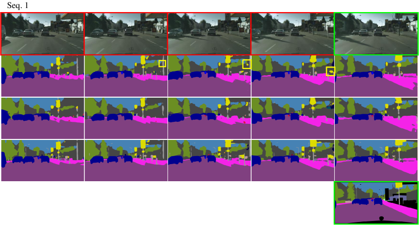
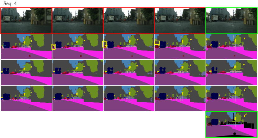
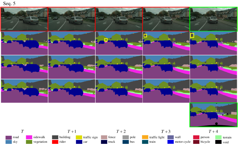
In recent years, remarkable success has been made by deep convolutional neural network (CNN) models in image parsing tasks [3, 5, 21, 28, 29, 34, 43, 44]. Some of those CNN models are thus proposed to be used for parsing scene videos frame by frame. However, as illustrated in Figure 1, naively applying those methods suffers from noisy and inconsistent labeling results across frames, since the important temporal context cues are ignored. For example, in the second row of Figure 1, the top-left region of class building in the frame +4 is incorrectly classified as car, which is temporally inconsistent with the parsing result of its preceding frames. Besides, for current data-hungry CNN models, finely annotated video data are rather limited as collecting pixel-level annotation for long videos is very labor-intensive. Even in the very recent scene parsing dataset Cityscapes [4], there are only 2,975 finely annotated training samples vs. overall 180K video frames. Deep CNN models are prone to over-fitting the small training data and thus generalize badly in real applications.
To tackle these two problems, we propose a novel Parsing with prEdictive feAtuRe Learning (PEARL) approach which is both annotation-efficient and effective for VSP. By enforcing them to predict future frames based on historical ones, our approach guides CNNs to learn powerful spatiotemporal features that implicitly capture video dynamics as well as high-level context like structures and motions of objects. Attractively, such a learning process is nearly annotation-free as it can be performed using any unlabeled videos. After this, our approach further adaptively integrates the obtained temporal-aware CNN to steer any image scene paring models to learn more spatial-temporally discriminative frame representations and thus enhance video scene parsing performance substantially.
Concretely, there are two novel components in our proposed approach: predictive feature learning and prediction steering parsing. As shown in Figure 1, given frames to , predictive feature learning aims to learn discriminative spatiotemporal features by enforcing a CNN model to predict the future frame as well as the parsing map of if available. Such predictive learning enables the CNN model to learn features capturing the cross-frame object structures, motions and other temporal cues, and provide better video parsing results, as demonstrated in the third row of Figure 1. To further adapt the obtained CNN along with its learned features to the parsing task, our approach introduces a prediction steering parsing architecture. Within this architecture, the temporal-aware CNN (trained by frame prediction) is utilized to guide an image-parsing CNN model to parse the current frame by providing temporal cues implicitly. The two parsing networks are jointly trained end-to-end and provide parsing results with strong cross-frame consistency and richer local details (as shown in the bottom row of Figure 1).
We conduct extensive experiments over two challenging datasets and compare our approach with strong baselines, i.e., state-of-the-art VGG16 [33] and Res101 [10] based parsing models. Our approach achieves the best results on both datasets. In the comparative study, we demonstrate its superiority to other methods that model temporal context, e.g., using optical flow [27].
To summarize, we make the following contributions to video scene parsing:
-
•
A novel predictive feature learning method is proposed to learn the spatiotemporal features and high-level context from a large amount of unlabeled video data.
-
•
An effective prediction steering parsing architecture is presented which utilizes the temporal consistent features to produce temporally smooth and structure preserving parsing maps.
-
•
Our approach achieves state-of-the-art performance on two challenging datasets, i.e., Cityscapes and Camvid.
2 Related Work
Recent image scene parsing progress is mostly stimulated by various new CNN architectures, including the fully convolutional architecture (FCN) with multi-scale or larger receptive fields [5, 21, 34] and the combination of CNN with graphical models [3, 28, 43, 44, 29]. There are also some recurrent neural networks based models [12, 17, 26, 32, 39]. However, without incorporating the temporal information when directly applying them to every frame of videos, the parsing results commonly lack cross-frame consistency and the quality is not good.
To utilize temporal consistency across frames, the motion and structure features in 3D data are employed by [6, 35, 42]. In addition, [9, 14, 16, 23] use CRF to model spatiotemporal context. However, those methods suffer from high computation cost as they need to perform expensive inference of CRF. Some other methods employ optical flow to capture the temporal consistency explored in [11, 30]. Different from above works that heavily depend on labeled data for supervised learning, our proposed approach takes advantage of both the labeled and unlabeled video sequences to learn richer temporal context information.
Generative adversarial networks were firstly introduced in [8] to generate natural images from random noises, and have been widely used in many fields including image synthesis [8], frame prediction [22, 24] and semantic inpainting [25]. Our approach also uses adversarial loss to learn more robust spatiotemporal features in frame predictions. Our approach is more related to [22, 24] by using adversarial training for frame prediction. However, different from [22, 24], PEARL tackles the VSP problem by utilizing spatiotemporal features learned in frame prediction.
3 Predictive Feature Learning for VSP
3.1 Motivation and Notations
The proposed approach is motivated by two challenging problems of video scene parsing: first, how to leverage the temporal context information to enforce cross-frame smoothness and produce structure preserving parsing results; second, how to build effective parsing models even in presence of insufficient training data.
Our approach solves these two problems through a novel predictive feature learning strategy. We consider the partially-labeled video collection used for predictive feature learning, denoted as , where denotes the raw video frames and denotes the provided dense annotations for a subset of . Here as collecting large-scale annotation is not easy. denotes the ground truth category at location in which is the number of semantic categories. Correspondingly, let and denote predicted frames and predicted parsing maps, respectively. We use to denote the preceding frames ahead of . For the first several frames in a video, we define their preceding set as if .
Video scene parsing can be formulated as seeking a parsing function that maps any frame sequence to the parsing map of the most recent frame:
| (1) |
The above definition reveals the difference between static scene image parsing and video scene parsing — the video scene parsing model has access to historical/temporal information for parsing the current target. We also want to highlight an important difference between our problem setting and some existing works [9, 23]: instead of using the whole video (including both past and future frames w.r.t. ) to parse the frame , we aim to perform parsing based on causal inference (or online inference) where only past frames are observable. This setting aligns better with real-time applications like autonomous driving where future frames cannot be seen in advance.
3.2 Predictive Feature Learning
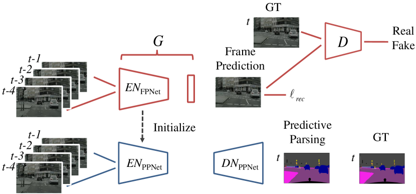
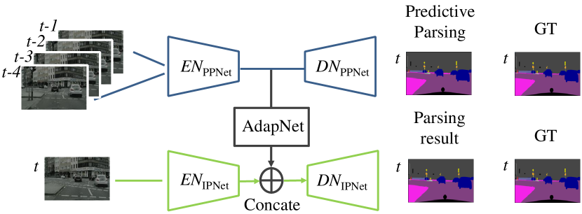
Predictive feature learning aims to learn spatiotemporal features capturing high-level context like object motions and structures from two consecutive predictive learning tasks, i.e., the frame prediction and the predictive parsing. Figure 2 gives an overview. In the first task, we train an FPNet for future frame prediction given several past frames by a new generative adversarial learning framework developed upon GANs [8, 24]. Utilizing a large amount of unlabeled video sequence data, the FPNet is capable of learning rich spatiotemporal features to model the variability of content and dynamics of videos. Then we further augment FPNet through Predictive Parsing, i.e. predicting parsing results of the future frame given previous frames. This adapts FPNet to another model (called PPNet) suitable for parsing.
Frame Prediction
The architecture of FPNet is illustrated in Figure 2a. It consists of two components, i.e., the generator (denoted as ) which generates future frame based on its preceding frames , and the discriminator (denoted as ) which plays against by trying to identify predicted frame and the real one . There is an Encoder (EN in Figure 2a) which maps the input video sequence to spatiotemporal features and a followed output layer to produce the RGB values of the predicted frame using the learned features. Note that Encoder can choose any deep networks with various architectures, e.g. VGG16 and Res101. We adapt them to be compatible with video inputs by using group convolution [13] for the first convolutional layer, where the group number is equal to the number of input past frames.
FPNet alternatively trains and for predicting frames with progressively improved quality. Denote learnable parameters of and as and respectively. The objective for training is to minimize the following binary cross-entropy loss where is fixed:
| (2) |
Minimizing the above loss gives a stronger discriminative ability to distinguish the predicted frames from real ones , enforcing to predict future frames with higher quality. Towards this target, learns to predict future frames more like real ones through
| (3) |
where
Minimizing the combination of reconstruction loss and adversarial loss supervises to predict the frame that looks both similar to its corresponding real frame and sufficiently authentic to fool the strong competitor . Our proposed frame prediction model is substantially different from vanilla GAN and more tailored for VSP problems. The key difference lies in the generator that takes past frame sequence as input to predict the future frame, instead of crafting new samples completely from random noise as vanilla GANs. Therefore, the future frames coming from such “temporally conditioned” FPNet should present certain temporal consistency with past frames. On the other hand, FPNet can learn representations containing implicit temporal cues desired for solving VSP problems.
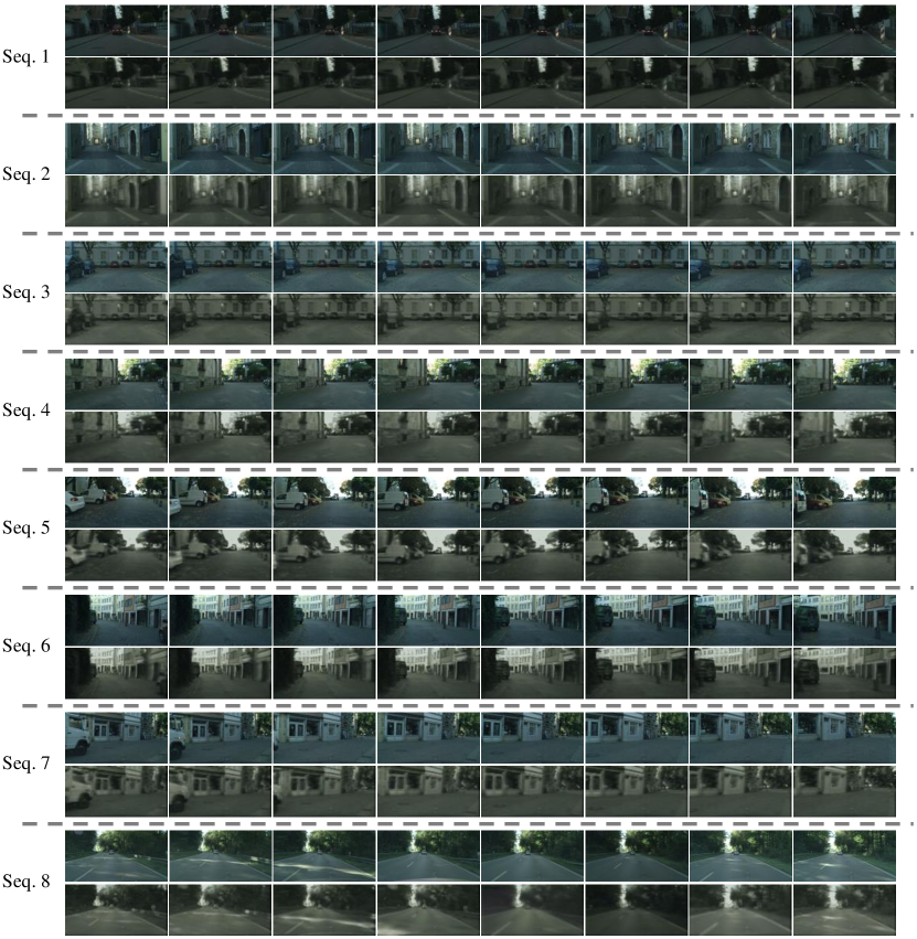
As illustrated by Figure 3, FPNet produces real-looking frame predictions by learning both the content and dynamics in videos. By comparing with the ground truth frame, the prediction frame resembles both the structures of objects/stuff like building/vegetation and the motion trajectories of cars, demonstrating that FPNet learns robust and generalized spatiotemporal features from video data.
In our experiments, we use a GoogLeNet [36] as and we try both Res101 and VGGNet for . More details are given in Section 4.1.

Predictive Parsing
The features learned by FPNet so far are trained for video frame generation. To adapt these spatiotemporal features to VSP problems, FPNet performs the second predictive learning task, i.e., predicting the parsing map of one frame given only its preceding frames (without seeing the frame to parse). This predictive parsing task is very challenging as we do not have any information of the current video frame.
Also, directly training FPNet for this predictive parsing task from scratch will not succeed. There are no enough data with annotations for training a good model free of over-fitting. Thus, training FPNet for frame prediction at first gives a good starting model for accomplishing the second task. In this perspective, frame prediction training is important for both spatiotemporal feature learning and feature adaption.
Details on how FPNet performs the predictive parsing task are given in Figure 2a. For predicting parsing maps, we modify the architecture of FPNet as follows. We remove the component from FPNet as well as the output layer in . Then we add a deconvNet (i.e. DN in the figure) on top of modified , which produces the parsing map sharing the same size with frames. We call this new FPNet as PPNet, short for Predictive Parsing Net.
More details about the structure of PPNet are given in Section 4.1. Based on the notations given in Section 3.1, the objective function for training PPNet is defined as
| (4) |
where denotes the per-pixel logarithmic probability predicted by PPNet for the category label . We introduce the weight vector to balance scene classes with different frequency in the training set. We will further discuss its role in the experiments.
Examples of predicted parsing maps from PPNet are shown in Figure 1 (the third row). Compared with parsing results from a traditional CNN parsing model on the single frame, the parsing maps of PPNet present two distinct properties. First, the parsing maps are temporally smooth which are reflected in the temporally consistent parsing results of regions like building where CNN models produce noisy and inconsistent parsing results. This demonstrates the PPNet indeed learns the temporally continuous dynamics from the video data. Secondly, PPNet tends to miss objects of small sizes, e.g., transport signs and poles. One reason is the inevitable blurry prediction [24] since the high frequency spectrum is prone to being smoothed. This problem can be mitigated by parsing at multiple scales [2] and we will investigate in the future.
In contrast, the conventional image parsing network relies on locally discriminative features such that it can capture small objects. However, due to lacking temporal information, its produced parsing maps are noisy and lack temporal consistency with past frames. Above observations motivate us to combine the strengths of PPNet and the CNN-based image parsing model to improve the overall VSP performance. Therefore, we develop the following prediction steering parsing architecture.
3.3 Prediction Steering Parsing
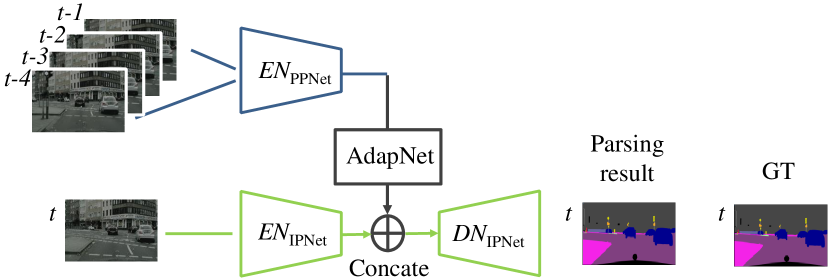
To take advantage of the temporally consistent spatiotemporal features learned by PPNet, we propose a novel architecture to integrate PPNet and the traditional image parsing network (short for IPNet) into a unified framework, called PSPNet, short for Prediction Steering Parsing Net.
As illustrated in Figure 2b, PSPNet has two inter-connected branches: one is the PPNet for predictive feature learning and the other is IPNet for frame-by-frame parsing. Similar to FPNet, the IPNet can also be chosen freely from any existed image parsing networks, e.g. FCN [21] and DeepLab [2]. As a high-level description, IPNet consists of two components, a feature encoder Encoder (EN) which transforms the input frame to dense pixel features and a deconvNet (DN) that produces per-pixel parsing map. Through an AdapNet (a shallow CNN), PPNet communicates its features to IPNet and steers the overall parsing process. In this way, the integrated features within IPNet gain two complementary properties, i.e., descriptiveness for the temporal context and discriminability for different pixels within a single frame. Therefore the overall PSPNet model is capable of producing more accurate video scene parsing results than both PPNet and IPNet. Formally, the objective function of training PSPNet end-to-end is defined as
| (5) |
where denotes the per-pixel logarithmic probability produced by the DN and balances the effect of PPNet and IPNet. We start training PSPNet by taking the trained PPNet in predictive parsing as initialization. We find this benefits the convergence of PSPNet training. In Section 4.2.1, we give more empirical studies.
Now we proceed to explain the role of AdapNet. There are two disadvantages by naively combining the intermediate features of PPNet and IPNet. Firstly, since the output features from those two feature encoders generally have different distributions, naively concatenating features harms the final performance as the “large” features dominate the “smaller” ones. Although during training, the followed weights in deconvNet may adjust accordingly, it requires careful tuning of parameters thus is subject to trial and error to find the best settings. Similar observations have been made in previous literature [19]. However, different from [19] which uses a normalization layer to tackle the scale problem, we use a more powerful AdapNet to transform the features of PPNet to be with proper norm and scale. Secondly, the intermediate features of PPNet and IPNet are with different semantic meanings, which means they reside in different manifold spaces. Therefore naively combining them increases the difficulty of learning the transformation from feature space to parsing map in the followed DN. By adding the AdapNet to convert the feature space in advance, it eases the training of DN. Detailed explorations of the architecture of AdapNet follows in Section 4.2.1.
3.4 Discussion
Unsupervised Feature Learning
Currently we train FPNet in a pseudo semi-supervised way, i.e. initialize and with ImageNet pre-trained models for faster training. Without using the pre-trained models, our approach becomes an unsupervised feature learning one. We also investigate the fully unsupervised learning strategy of FPNet in the experiments. The resulting FPNet is denoted as FPNet. As shown in Table LABEL:table:step123_cmp, FPNet performs similarly well as FPNet using the pre-trained VGG16 model. In the future, we will perform unsupervised learning on FPNet using deeper architectures and further improve its ability.
Proactive Parsing
Our predictive learning approach recalls another challenging but attractive task, i.e., to predict the future parsing maps for a few seconds without seeing them, only based on past frames. Achieving this allows autonomous vehicles or other parsing-demanded devices to receive parsing information ahead and get increased buffer time for decision making. Our approach indeed has the potential to accomplish this proactive parsing task. As one can observe from Figure 1, the predicted parsing maps capture the temporal information across frames, such as motions of cars, and the predicted parsing map reflects such dynamics and shows roughly correct prediction. In the future, we will investigate how to enhance the performance of our approach on predictive parsing to get higher-quality and longer-term future results.
4 Experiments
4.1 Settings and Implementation Details
Datasets
Since PEARL tackles the scene parsing problem with temporal context, we choose Cityscapes [4] and Camvid [1] for evaluation. Both datasets provide annotated frames as well as adjacent frames, suitable for testing the temporal modeling ability. Cityscapes is a large-scale dataset containing finely pixel-wise annotations on 2,975/500/1,525 train/val/test frames with 19 semantic classes and another 20,000 coarsely annotated frames. Each finely annotated frame is sampled from the 20th frame of a 30-frame video clip in the dataset, giving in total 180K frames. Since there are no video data provided for the coarsely annotated frames, we only use finely annotated ones for training PEARL. Every frame in Cityscapes has a resolution of 10242048 pixels.
The Camvid dataset contains 701 color images with annotations on 11 semantic classes. These images are extracted from driving videos captured at daytime and dusk. Each video contains 5,000 frames on average, with a resolution of 720960 pixels, giving in total 40K frames.
Baselines
We conduct experiments to compare PEARL with two baselines which use different deep network architectures.
-
•
VGG16-baseline Our VGG16-baseline is built upon DeepLab [3]. We make the following modifications. We add three deconvolutional layers after fc7 to learn better transformations to label maps. The architectures of three added deconvolutional layers in VGG16-baseline are , and respectively. Here denotes output feature maps, denotes the kernel size of , denotes a stride of length and denotes the padding size of . The layers before fc7 (included) constitute the encoder network (EN in Figure 2) and the other layers form the decoder network (DN in Figure 2).
-
•
Res101-baseline Our Res101-baseline is modified from [10] by adapting it to a fully convolutional network following [21]. Specifically, we replace the average pooling layer and the 1000-way classification layer with a fully convolutional layer to produce dense label maps. Also, we modify conv5_1, conv5_2 and conv5_3 to be dilated convolutional layers by setting their dilation size to be 2 to enlarge the receptive fields. As a result, the output feature maps of conv5_3 have a stride of 16. Following [21], we utilize high-frequency features learned in bottom layers by adding skip connections from conv1, pool1, conv3_3 to corresponding up-sampling layers to produce label maps with the same size as input frames. The layers from conv1 to conv5_3 belong to EN while the other layers belong to DN. Following [40], we also use hard training sample mining to reduce over-fitting.
Note that IPNets in PEARL share the same network architectures as baseline models. The encoder networks in FPNet/PPNet and the decoder network in PPNet share the same network architectures of the encoder network and the decoder network in baseline models, respectively.
Evaluation Metrics
Following previous practice, we use the mean IoU (mIoU) for Cityscapes, and per-pixel accuracy (PA) and average per-class accuracy (CA) for Camvid. In particular, mIoU is defined as the pixel intersection-over-union (IOU) averaged across all categories; PA is defined as the percentage of all correctly classified pixels; and CA is the average of all category-wise accuracies.
Implementation Details
Throughout the experiments, we set the number of preceding frames of each frame as 4, i.e., in (ref. Section 3.1 in the main text). When training FPNet, we randomly select frame sequences from those with a length of 4 and also enough movement (the distance between the raw frames is larger than a threshold ). In this way, we finally obtain 35K/8.8K sequences from Cityscapes and Camvid respectively. The input frames for training FPNet are all normalized such that values of their pixels lie between -1 and 1. For training PPNet and PSPNet, we only perform mean value subtraction on the frames. For training PPNet, we select the 4 frames before the annotated images to form the training sequences, where the frames are required to have sufficient motion, consistent with FPNet.
We perform random cropping and horizontal flipping to augment the training frames for FPNet, PPNet and PSPNet. In addition, for training FPNet, the temporal order of a sequence (including the to-predict frame and 4 preceding frames) is randomly reversed to model various dynamics in videos. The hyperparameters in PEARL are fixed as in Eq. (3) and in Eq. (3.3) and the probability threshold of hard training sample mining in Res101-baseline as 0.9. The values are chosen through cross-validation.
Since the class distribution is extremely unbalanced, we increase the weight of rare classes during training, similar to [5, 12, 32]. In particular, we adopt the re-weighting strategy in [32]. The weight for the class is set as where is the frequency of class and is a dataset-dependent scalar, which is defined according to the 85%/15% frequent/rare classes rule.
All of our experiments are carried out on NVIDIA Titan X and Tesla M40 GPUs using Caffe library.
Computational Efficiency
Since no post-processing is required in PEARL, the running time of PEARL for obtaining the parsing map of a frame with resolution 1,0242,048 is only 0.8 seconds on a modern GPU, among the fastest methods in existing works.

4.2 Results
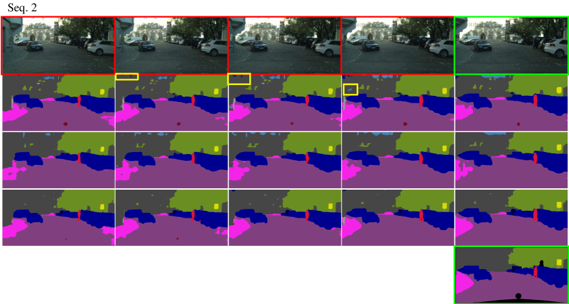
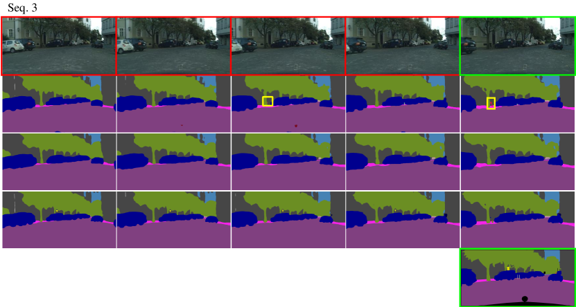
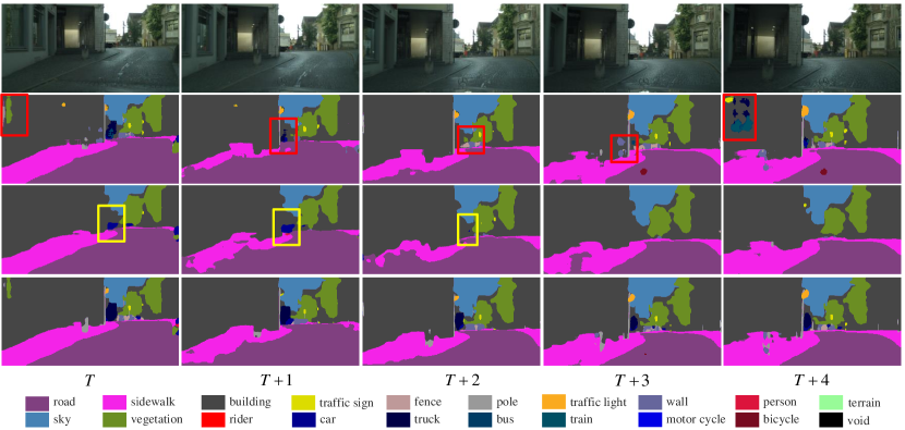
Examples of parsing maps produced by PEARL are illustrated in Figure 4, where VGG16 is used in both the baseline model and PEARL. As can be seen from Figure 4, compared with the baseline model, PEARL produces smoother parsing maps, e.g. for the class vegetation, and stronger discriminability for small objects, e.g. for the classes pole, pedestrian, traffic sign as highlighted in red boxes. Such improvements are attributed to the capability of PEARL to learn the temporally consistent features and discriminative features for local pixel variance simultaneously.
4.2.1 Cityscapes
Ablation Analysis
We investigate contribution of each component of our approach.
(1) Predictive Feature Learning. To investigate the contribution of the two predictive feature learning networks, FPNet and PPNet, we conduct three experiments. The comparison results are listed in Table LABEL:table:step123_cmp, where the front-CNN of FPNet and PPNet both use the VGG16 architecture.
First, we would like to verify the effectiveness of the features learned by
FPNet for VSP. We concatenate the output features (denoted as
feat) of Encoder with the
output features of Encoder in IPNet, as shown in
Figure 2c, and fix the
Encoder during training. In this way, the FPNet only
extracts spatiotemporal features for the IPNet. As can be seen from
Table LABEL:table:step123_cmp, by combining feat, the
mIoU increases from 63.4 (of the VGG16-baseline) to 68.6, demonstrating FPNet
indeed learns useful spatiotemporal features through frame prediction.
Similarly, we replace Encoder in the above experiment
with Encoder to investigate the influence of PPNet on
final performance. In the experiment, the per-pixel cross-entropy loss layer of
PPNet is removed and the weights of Encoder are
fixed. As illustrated in Table LABEL:table:step123_cmp, combining IPNet with
feat further increases the mIoU by 0.5 compared to
combining feat, demonstrating features learned by PPNet
from predictive parsing are useful for VSP.
Finally, we look into the effectiveness of joint training of PPNet and IPNet. It is observed from Table LABEL:table:step123_cmp that the resulting model, i.e. PEARL achieves the best performance, benefiting from the joint end-to-end training strategy.
| Methods | mIoU |
| VGG16-baseline | 63.4 |
feat + IPNet
|
68.6 |
feat + IPNet
|
68.4 |
feat + IPNet
|
69.1 |
| PEARL | 69.8 |
| Methods | mIoU |
|---|---|
| VGG16-baseline | 63.4 |
feat + IPNet
|
64.5 |
| PEARL | 69.8 |
| Res101-baseline | 72.5 |
feat + IPNet
|
72.7 |
| PEARL | 74.9 |
| Methods |
road |
sidewalk |
building |
wall |
fence |
pole |
traffic light |
traffic sign |
vegetation |
terrain |
sky |
person |
rider |
car |
truck |
bus |
train |
motorcycle |
bicycle |
mIoU |
|---|---|---|---|---|---|---|---|---|---|---|---|---|---|---|---|---|---|---|---|---|
| FCN_8s [21] | 97.4 | 78.4 | 89.2 | 34.9 | 44.2 | 47.4 | 60.1 | 65.0 | 91.4 | 69.3 | 93.9 | 77.1 | 51.4 | 92.6 | 35.3 | 48.6 | 46.5 | 51.6 | 66.8 | 65.3 |
| DPN [20] | 97.5 | 78.5 | 89.5 | 40.4 | 45.9 | 51.1 | 56.8 | 65.3 | 91.5 | 69.4 | 94.5 | 77.5 | 54.2 | 92.5 | 44.5 | 53.4 | 49.9 | 52.1 | 64.8 | 66.8 |
| Dilation10 [41] | 97.6 | 79.2 | 89.9 | 37.3 | 47.6 | 53.2 | 58.6 | 65.2 | 91.8 | 69.4 | 93.7 | 78.9 | 55.0 | 93.3 | 45.5 | 53.4 | 47.7 | 52.2 | 66.0 | 67.1 |
| DeepLab [2] | 97.9 | 81.3 | 90.3 | 48.8 | 47.4 | 49.6 | 57.9 | 67.3 | 91.9 | 69.4 | 94.2 | 79.8 | 59.8 | 93.7 | 56.5 | 67.5 | 57.5 | 57.7 | 68.8 | 70.4 |
| Adelaide [18] | 98.0 | 82.6 | 90.6 | 44.0 | 50.7 | 51.1 | 65.0 | 71.7 | 92.0 | 72.0 | 94.1 | 81.5 | 61.1 | 94.3 | 61.1 | 65.1 | 53.8 | 61.6 | 70.6 | 71.6 |
| LRR-4X [7] | 97.9 | 81.5 | 91.4 | 50.5 | 52.7 | 59.4 | 66.8 | 72.7 | 92.5 | 70.1 | 95.0 | 81.3 | 60.1 | 94.3 | 51.2 | 67.7 | 54.6 | 55.6 | 69.6 | 71.8 |
| PEARL111https://www.cityscapes-dataset.com/method-details/?submissionID=328(ours) | 98.3 | 83.9 | 91.6 | 47.6 | 53.4 | 59.5 | 66.8 | 72.5 | 92.7 | 70.9 | 95.2 | 82.4 | 63.5 | 94.7 | 57.4 | 68.8 | 62.2 | 62.6 | 71.5 | 73.4 |
(2) Comparison with Optical Flow Methods. To verify the superiority of PEARL on learning the temporal information specific for VSP, we compare PEARL with other temporal context modeling methods. First, we naively pass each frame in and through baseline models (both VGG16-baseline and Res101-baseline) and merge their probability maps to obtain the final label map of . It is verified by experiments that such methods achieve worse performance than baseline models due to their weakness of utilizing temporal information and the noisy probability map produced for each frame. Since optical flow is naturally capable of modeling the temporal information in videos, we use it as a strong baseline to compete with PEARL. We employ the epic flow [27] for computing all optical flows. Then we warp the parsing map of the frame and merge it with that of the frame , according to the optical flow calculated between these two frames. In this way, the temporal context is modeled explicitly via optical flow. This method performs better than the last method but its performance is still inferior to baseline models. It is because the CNN models produce the parsing map without knowing the temporal information during training.
Then we conduct the third experiment by concatenating the optical flows
calculated from to with the frame , which forms 5-channel
raw data (RGB plus X/Y channels of optical flow). Based on optical flow
augmented data, we re-train baseline models. During training, each kernel in the
first convolutional layer of baseline models is randomly initialized for the
weights corresponding to the X/Y channels of optical flow. This method is
referred to as “feat + IPNet”. The comparative results of
“feat + IPNet” and PEARL using VGG16 and Res101 are
displayed in Table 2. From the results, one can observe
“feat + IPNet” achieves higher performance than baselines
models as it uses temporal context during training. Notably, PEARL significantly
beats “feat + IPNet” on both network architectures, proving
its superior ability to model temporal information for VSP problems.
(3) Ablation Study of AdapNet As introduced in Section 3.3, AdapNet improves the performance of PEARL by learning the latent transformations from Encoder to Encoder. In our experiments, the AdapNet contains one convolutional layer followed by ReLU. The kernel size of the convolutional layer is 1 and the number of kernels is equal to that of output channels of Encoder. Compared to the PEARL w/o AdapNet, adding AdapNet brings 1.1/0.3 mIoU improvements for PEARL and PEARL, respectively. We also conduct experiments by increasing convolutional layers of AdapNet, but only observe marginal improvements. Since deeper AdapNet brings more computation cost, we use AdapNet with one convolutional layer.
Comparison with State-of-the-arts
The comparison of PEARL with other state-of-the-arts on Cityscapes val set is listed in Table 4, from which one can observe PEARL achieves the best performance among all compared methods on both network architectures. Note loss re-weighting is not used on this dataset.
Specifically, PEARL and PEARL significantly improve the corresponding baseline models by 6.4/2.4 mIoU, respectively. Notably, compared with [31] which proposed a temporal skip network based on VGG16 for video scene parsing, PEARL beats it by 5.4 in terms of mIoU. We also note that different from other methods which extensively modify VGG16 networks to enhance its discriminative power for image parsing, e.g. [2, 18], our PEARL is built on vanilla VGG16 architecture. Thus it is reasonable to expect further improvement on the VSP performance by using more powerful base network architectures. Furthermore, we submit PEARL to the online evaluation server of Cityscapes to compare with other state-of-the-arts on Cityscapes test set. As shown in Table 3, our method achieves the best performance among all top methods which have been published till the time of submission. Note in inference, PEARL only uses single-scale testing without CRF post-processing for the sake of fast inference.
4.2.2 Camvid
We further investigate the effectiveness of PEARL on Camvid. Its result and the best results ever reported on this dataset are listed in Table 5. Following [12, 32], loss re-weighting is used on this dataset. One can observe that PEARL performs much better than all competing methods — significantly improving the PA/CA of the baseline model (Res101-basline) by 1.6%/2.5% respectively, once again demonstrating its strong capability of improving VSP performance. Notably, compared to the optical flow based methods [16] and [20] which utilize CRF to model temporal information, PEARL shows great advantages in performance, verifying its superiority in modeling the spatiotemporal context for VSP problems.
5 Conclusion
We proposed a predictive feature learning method for effective video scene parsing. It contains two novel components: predictive feature learning and prediction steering parsing. The first component learns spatiotemporal features by predicting future frames and their parsing maps without requiring extra annotations. The prediction steering parsing architecture then guides the single frame parsing network to produce temporally smooth and structure preserving results by using the predictive feature learning outputs. Extensive experiments on Cityscapes and Camvid fully demonstrated the effectiveness of our approach.
References
- [1] G. J. Brostow, J. Shotton, J. Fauqueur, and R. Cipolla. Segmentation and recognition using structure from motion point clouds. In ECCV. 2008.
- [2] L. Chen, G. Papandreou, I. Kokkinos, K. Murphy, and A. L. Yuille. Deeplab: Semantic image segmentation with deep convolutional nets, atrous convolution, and fully connected crfs. CoRR, abs/1606.00915, 2016.
- [3] L.-C. Chen, G. Papandreou, I. Kokkinos, K. Murphy, and A. L. Yuille. Semantic image segmentation with deep convolutional nets and fully connected crfs. In ICLR, 2015.
- [4] M. Cordts, M. Omran, S. Ramos, T. Rehfeld, M. Enzweiler, R. Benenson, U. Franke, S. Roth, and B. Schiele. The cityscapes dataset for semantic urban scene understanding. arXiv preprint arXiv:1604.01685, 2016.
- [5] C. Farabet, C. Couprie, L. Najman, and Y. LeCun. Learning hierarchical features for scene labeling. Pattern Analysis and Machine Intelligence, IEEE Transactions on, 35(8):1915–1929, 2013.
- [6] G. Floros and B. Leibe. Joint 2d-3d temporally consistent semantic segmentation of street scenes. In CVPR, pages 2823–2830. IEEE, 2012.
- [7] G. Ghiasi and C. C. Fowlkes. Laplacian reconstruction and refinement for semantic segmentation. CoRR, abs/1605.02264, 2016.
- [8] I. Goodfellow, J. Pouget-Abadie, M. Mirza, B. Xu, D. Warde-Farley, S. Ozair, A. Courville, and Y. Bengio. Generative adversarial nets. In NIPS, pages 2672–2680, 2014.
- [9] B. L. . X. H. . S. Gould. Multi-class semantic video segmentation with exemplar-based object reasoning. In WACV, 2016.
- [10] K. He, X. Zhang, S. Ren, and J. Sun. Deep residual learning for image recognition. arXiv preprint arXiv:1512.03385, 2015.
- [11] J. Hur and S. Roth. Joint optical flow and temporally consistent semantic segmentation. In ECCV, pages 163–177. Springer, 2016.
- [12] X. Jin, Y. Chen, J. Feng, Z. Jie, and S. Yan. Multi-path feedback recurrent neural network for scene parsing. CoRR, abs/1608.07706, 2016.
- [13] A. Krizhevsky, I. Sutskever, and G. E. Hinton. Imagenet classification with deep convolutional neural networks. In NIPS, pages 1097–1105, 2012.
- [14] A. Kundu, V. Vineet, and V. Koltun. Feature space optimization for semantic video segmentation. In CVPR, 2016.
- [15] L. Ladickỳ, P. Sturgess, K. Alahari, C. Russell, and P. H. Torr. What, where and how many? combining object detectors and crfs. In ECCV. 2010.
- [16] P. Lei and S. Todorovic. Recurrent temporal deep field for semantic video labeling. In ECCV, pages 302–317. Springer, 2016.
- [17] M. Liang, X. Hu, and B. Zhang. Convolutional neural networks with intra-layer recurrent connections for scene labeling. In NIPS, 2015.
- [18] G. Lin, C. Shen, A. v. d. Hengel, and I. Reid. Exploring context with deep structured models for semantic segmentation. arXiv preprint arXiv:1603.03183, 2016.
- [19] W. Liu, A. Rabinovich, and A. C. Berg. Parsenet: Looking wider to see better. arXiv preprint arXiv:1506.04579, 2015.
- [20] Z. Liu, X. Li, P. Luo, C.-C. Loy, and X. Tang. Semantic image segmentation via deep parsing network. In ECCV, pages 1377–1385, 2015.
- [21] J. Long, E. Shelhamer, and T. Darrell. Fully convolutional networks for semantic segmentation. In CVPR, 2015.
- [22] W. Lotter, G. Kreiman, and D. Cox. Unsupervised learning of visual structure using predictive generative networks. arXiv preprint arXiv:1511.06380, 2015.
- [23] B. Mahasseni, S. Todorovic, and A. Fern. Approximate policy iteration for budgeted semantic video segmentation. CoRR, abs/1607.07770, 2016.
- [24] M. Mathieu, C. Couprie, and Y. LeCun. Deep multi-scale video prediction beyond mean square error. arXiv preprint arXiv:1511.05440, 2015.
- [25] D. Pathak, P. Krahenbuhl, J. Donahue, T. Darrell, and A. A. Efros. Context encoders: Feature learning by inpainting. arXiv preprint arXiv:1604.07379, 2016.
- [26] P. H. Pinheiro and R. Collobert. Recurrent convolutional neural networks for scene parsing. arXiv preprint arXiv:1306.2795, 2013.
- [27] J. Revaud, P. Weinzaepfel, Z. Harchaoui, and C. Schmid. Epicflow: Edge-preserving interpolation of correspondences for optical flow. In CVPR, pages 1164–1172, 2015.
- [28] A. Roy and S. Todorovic. Scene labeling using beam search under mutex constraints. In CVPR, 2014.
- [29] A. G. Schwing and R. Urtasun. Fully connected deep structured networks. arXiv preprint arXiv:1503.02351, 2015.
- [30] L. Sevilla-Lara, D. Sun, V. Jampani, and M. J. Black. Optical flow with semantic segmentation and localized layers. arXiv preprint arXiv:1603.03911, 2016.
- [31] E. Shelhamer, K. Rakelly, J. Hoffman, and T. Darrell. Clockwork convnets for video semantic segmentation. arXiv preprint arXiv:1608.03609, 2016.
- [32] B. Shuai, Z. Zuo, G. Wang, and B. Wang. Dag-recurrent neural networks for scene labeling. arXiv preprint arXiv:1509.00552, 2015.
- [33] K. Simonyan and A. Zisserman. Very deep convolutional networks for large-scale image recognition. arXiv preprint arXiv:1409.1556, 2014.
- [34] R. Socher, C. C. Lin, C. Manning, and A. Y. Ng. Parsing natural scenes and natural language with recursive neural networks. In ICML, 2011.
- [35] P. Sturgess, K. Alahari, L. Ladicky, and P. H. Torr. Combining appearance and structure from motion features for road scene understanding. In BMVC, 2009.
- [36] C. Szegedy, W. Liu, Y. Jia, P. Sermanet, S. Reed, D. Anguelov, D. Erhan, V. Vanhoucke, and A. Rabinovich. Going deeper with convolutions. arXiv preprint arXiv:1409.4842, 2014.
- [37] J. Tighe and S. Lazebnik. Superparsing: scalable nonparametric image parsing with superpixels. In ECCV. 2010.
- [38] J. Uhrig, M. Cordts, U. Franke, and T. Brox. Pixel-level encoding and depth layering for instance-level semantic labeling. arXiv preprint arXiv:1604.05096, 2016.
- [39] F. Visin, K. Kastner, A. C. Courville, Y. Bengio, M. Matteucci, and K. Cho. Reseg: A recurrent neural network for object segmentation. CoRR, abs/1511.07053, 2015.
- [40] Z. Wu, C. Shen, and A. van den Hengel. High-performance semantic segmentation using very deep fully convolutional networks. CoRR, abs/1604.04339, 2016.
- [41] F. Yu and V. Koltun. Multi-scale context aggregation by dilated convolutions. arXiv preprint arXiv:1511.07122, 2015.
- [42] C. Zhang, L. Wang, and R. Yang. Semantic segmentation of urban scenes using dense depth maps. In ECCV, pages 708–721. Springer, 2010.
- [43] Y. Zhang and T. Chen. Efficient inference for fully-connected crfs with stationarity. In CVPR, 2012.
- [44] S. Zheng, S. Jayasumana, B. Romera-Paredes, V. Vineet, Z. Su, D. Du, C. Huang, and P. H. Torr. Conditional random fields as recurrent neural networks. In ICCV, 2015.
Appendix A Qualitative Evaluation of PEARL
A.1 More Results of Frame Prediction from FPNet in PEARL
Please refer to Figure 5;
A.2 More Results of Video Scene Parsing
Please refer to Figure 4.
