Flow polytopes with Catalan volumes

Abstract.

The Chan-Robbins-Yuen polytope can be thought of as the flow polytope of the complete graph with netflow vector $(1,0,\ldots,0,-1)$. The normalized volume of the Chan-Robbins-Yuen polytope equals the product of consecutive Catalan numbers, yet there is no combinatorial proof of this fact. We consider a natural generalization of this polytope, namely, the flow polytope of the complete graph with netflow vector $(1,1,0,\ldots,0,-2)$. We show that the volume of this polytope is a certain power of $2$ times the product of consecutive Catalan numbers. Our proof uses constant term identities and further deepens the combinatorial mystery of why these numbers appear. In addition we introduce two more families of flow polytopes whose volumes are given by product formulas.

1. Introduction

We underscore the wealth of flow polytopes with product formulas for volumes. The natural question arising from our study and previous work [13, 14, 2, 3, 10, 1, 8, 11] is: is there a unified (combinatorial?) explanation for these beautiful product formulas? All current results relating to these volumes show these formulas as a result of various computations that surprisingly yield products. Our hope is that by identifying three more distinguished families of flow polytopes with beautiful product formulas for their volumes we inch closer to uncovering an illuminating explanation for these formulas.

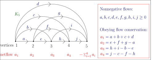
The flow polytope $\mathcal{F}_{G}({\bf a})$ is associated to a graph $G$ on the vertex set $\{1,\ldots,n\}$ with edges directed from smaller to larger vertices and netflow vector ${{\bf a}}=(a_{1},\ldots,a_{n})\in\mathbb{Z}^{n}$. The points of $\mathcal{F}_{G}({\bf a})$ are nonnegative flows on the edges of $G$ so that flow is conserved at each vertex; see Figure 1 (Section 2 has precise definition). Flow polytopes are closely related to Kostant partition functions [1, 10], Grothendieck polynomials [9, 4, 5], and the space of diagonal harmonics [11, 7], among others.

Figure 1. The flow polytope $\mathcal{F}_{K_{5}}(a_{1},a_{2},a_{3},a_{4},-\sum_{i=1}^{4}a_{i})$ consists of all points $(a,b,c,d,e,f,g,h,i,j)\in\mathbb{R}^{10}$ satisfying the inequalities and equations displayed to the right of  $K_{5}$.

Perhaps the most famous flow polytope is $\mathcal{F}_{K_{n+1}}(1,0,\ldots,0,-1)$, the flow polytope of the complete graph, also referred to as the Chan–Robbins–Yuen polytope ($CRY_{n}$) [3]. Chan, Robbins and Yuen defined $CRY_{n}$ as the convex hull of the set of $n\times n$ permutation matrices $\pi$ with $\pi_{ij}=0$ if $j\geq i+2$, which can be shown to be integrally equivalent to $\mathcal{F}_{K_{n+1}}(1,0,\ldots,0,-1)$. (Thus, $CRY_{n}$ and $\mathcal{F}_{K_{n+1}}(1,0,\ldots,0,-1)$ are combinatorially equivalent, and have the same volume and Ehrhart polynomial.) The polytope $CRY_{n}$ is a face of the Birkhoff polytope, the polytope of all doubly stochastic matrices, prominent in combinatorial optimization. Remarkably, the volume of the $CRY_{n}$ polytope is the product of the first $n-2$ Catalan numbers, as conjectured by Chan, Robbins and Yuen in [3] and proved by Zeilberger analytically in [13]. Under volume in this paper we mean the normalized volume of a polytope. The normalized volume of a $d$-dimensional polytope $P\subset\mathbb{R}^{n}$, denoted by ${\rm vol}\hskip 1.4457ptP$, is the volume form which assigns a volume of one to the smallest $d$-dimensional integer simplex in the affine span of $P$.

Several generalizations of $CRY_{n}$ are introduced and studied in [8, 10, 11]. The volume formulas of the aforementioned polytopes are akin that of $CRY_{n}$. In this paper we identify three new families of flow polytopes generalizing $CRY_{n}$. In particular, we study the flow polytope of the complete graph with netflow vector $(1,1,0,\ldots,0,-2)$ and show that its volume is a power of $2$ times the product of consecutive Catalan numbers. Furthermore, if we take the complete graph with various multiple edges and consider the corresponding flow polytope with netflow vectors $(1,0,\ldots,0,-1)$ or $(1,\ldots,1,-n)$ we still obtain product formulas for their volumes, as a result of the generalized Lidskii formulas [1] and the Morris (and the like) constant term identity [12]. Combinatorial proofs remain elusive, but all the more enticing.

Now we state our results regarding the three new families of polytopes we study in this paper. For definitions and background see Section 2.

Theorem 1.1.

The normalized volume of the flow polytope $\mathcal{F}_{K_{n+1}}(1,1,0,\ldots,0,-2)$ is

$${\rm vol}\mathcal{F}_{K_{n+1}}(1,1,0,\ldots,0,-2)=2^{{n\choose 2}-1}\prod_{i=1}^{n-2}\operatorname{Cat}(i),$$

where $\operatorname{Cat}(i)=\frac{1}{i+1}{2i\choose i}$ is the $i$th Catalan number.

Let $\Gamma(\cdot)$ denote the Gamma function. In particular, $\Gamma(j)=(j-1)!$ when $j\in\mathbb{N}$.

Theorem 1.2.

Denote by $K_{n+1}^{a,b,m}$ the graph on the vertex set $[n+1]$ with each edge $(1,i)$, $i\in[2,n]$, appearing $a$ times, edge $(i,n+1)$, $i\in[2,n]$, appearing $b$ times, and $(i,j)$, $1<i<j<n+1$ appearing $m$ times. Then we have that

$${\rm vol}\mathcal{F}_{K_{n+1}^{a,b,m}}(1,0,\ldots,0,-1)=\frac{1}{(n-1)!}\prod_{j=0}^{n-2}\frac{\Gamma(a-1+b+(n-2+j)\frac{m}{2})\Gamma(\frac{m}{2})}{\Gamma(a+j\frac{m}{2})\Gamma(b+j\frac{m}{2})\Gamma(\frac{m}{2}+j\frac{m}{2})}.$$

Theorem 1.3.

Denote by $K_{n+1}^{a,b}$ the graph on the vertex set $[n+1]$ with edges $(i,j)$, $1\leq i<j\leq n$, appearing with multiplicity $a$ and the edges $(i,n+1)$, $i\in[n]$, appearing with multiplicity $b$. For $n\geq 2$ and nonnegative integers $a,b$ we have that

$${\rm vol}\mathcal{F}_{K_{n+1}^{a,b}}(1,1,\ldots,1,-n)=\big{(}(b-1)n+a{\textstyle\binom{n}{2}}\big{)}!\prod_{i=0}^{n-1}\frac{\Gamma(1+a/2)}{\Gamma(1+(i+1)a/2)\Gamma(b+ia/2)}.$$

The polytope $\mathcal{F}_{K_{n+1}}(1,0,\ldots,0,-1)$ (integrally equivalent to $CRY_{n}$) belongs to the polytope family in Theorem 1.2. Indeed, Zeilberger [13] proved the $CRY_{n}$ volume formula by specializing Morris identity (stated in Lemma 4.1), while Theorem 1.2 uses the whole strength of Morris identity. Similarly, we make use of a Morris-type identity proved in [11] to prove Theorem 1.3. It is Theorem 1.1 that makes us work significantly: neither the Morris, nor the Morris-type identities mentioned above work, rather we prove a new constant term identity to tackle it.

The outline of the paper is as follows. In Section 2 we give the necessary definitions on flow polytopes. In Section 3 we prove Theorem 1.1. In Section 4 we prove Theorems 1.2 and in Section 5 we prove Theorem 1.3. Finally, in Section 6 we enumerate the vertices of the polytopes $\mathcal{F}_{K_{n+1}}(1,1,0,\ldots,0,-2)$ appearing in Theorem 1.1.

2. Flow polytopes $\mathcal{F}_{G}({\bf a})$ and Kostant partition functions

The exposition of this section follows that of [10]; see [10] for more details.

Let $G$ be a (loopless) graph on the vertex set $[n+1]$ with $N$ edges. To each edge $(i,j)$, $i<j$, of $G$, associate the positive type $A_{n}$ root ${\rm v}(i,j)={\bf e}_{i}-{\bf e}_{j}$, where ${\bf e}_{i}$ is the $i$th standard basis vector in $\mathbb{R}^{n+1}$. Let $S_{G}:=\{\{{\bf v}_{1},\ldots,{\bf v}_{N}\}\}$ be the multiset of roots corresponding to the multiset of edges of $G$. Let $M_{G}$ be the $(n+1)\times N$ matrix whose columns are the vectors in $S_{G}$. Fix an integer vector ${\bf a}=(a_{1},\ldots,a_{n+1})\in\mathbb{Z}^{n+1}$ which we call the netflow and for which we require that $a_{n+1}=-\sum_{i=1}^{n}a_{i}$. An ${\bf a}$-flow ${\bf f}_{G}$ on $G$ is a vector ${\bf f}_{G}=(b_{k})_{k\in[N]}$, $b_{k}\in\mathbb{R}_{\geq 0}$ such that $M_{G}{\bf f}_{G}={\bf a}$. That is, for all $1\leq i\leq n+1$, we have

(1) $$\sum_{e=(g<i)\in E(G)}b(e)+a_{i}=\sum_{e=(i<j)\in E(G)}b(e)$$

Define the flow polytope $\mathcal{F}_{G}({\bf a})$ associated to a graph $G$ on the vertex set $[n+1]$ and the integer vector ${\bf a}=(a_{1},\ldots,a_{n+1})$ as the set of all ${\bf a}$-flows ${\bf f}_{G}$ on $G$, i.e., $\mathcal{F}_{G}=\{{\bf f}_{G}\in\mathbb{R}^{N}_{\geq 0}\mid M_{G}{\bf f}_{G}={\bf a}\}$. The flow polytope $\mathcal{F}_{G}({\bf a})$ then naturally lives in $\mathbb{R}^{N}$, where $N$ is the number of edges of $G$. The vertices of the flow polytope $\mathcal{F}_{G}({\bf a})$ are the ${\bf a}$-flows whose supports are acyclic subgraphs of $G$ [6, Lemma 2.1].

Recall that the Kostant partition function $K_{G}$ evaluated at the vector ${\bf b}\in\mathbb{Z}^{n+1}$ is defined as

(2) $$K_{G}({\bf b})=\#\Big{\{}(c_{k})_{k\in[N]}\Bigm{|}\sum_{k\in[N]}c_{k}{\bf v}_{k}={\bf b}\textrm{ and }c_{k}\in\mathbb{Z}_{\geq 0}\Big{\}},$$

where $[N]=\{1,2,\ldots,N\}$.

The generating series of the Kostant partition function is

(3) $$\sum_{{\bf b}\in\mathbb{Z}^{n+1}}K_{G}({\bf b}){\bf x}^{\bf b}={\prod_{(i,j)\in E(G)}}(1-x_{i}x_{j}^{-1})^{-1},$$

where ${\bf x}^{\bf b}=x_{1}^{b_{1}}x_{2}^{b_{2}}\cdots x_{n+1}^{b_{n+1}}$. In particular,

(4) $$K_{K_{n+1}}({\bf b})=[{\bf x}^{\bf b}]\prod_{1\leq i<j\leq n+1}(1-x_{i}x_{j}^{-1})^{-1}.$$

Assume that ${\bf a}=(a_{1},a_{2},\ldots,a_{n})$ satisfies $a_{i}\geq 0$ for $i=1,\ldots,n$. Let ${\bf a}^{\prime}=(a_{1},a_{2},\ldots,a_{n},-\sum_{i=1}^{n}a_{i})$. The generalized Lidskii formulas of Baldoni and Vergne state that for a graph $G$ on the vertex set $[n+1]$ with $N$ edges we have

Theorem 2.1.

[1, Theorem 38]

(5) $${\rm vol}\mathcal{F}_{G}({\bf a^{\prime}})=\sum_{{\bf i}}\binom{N-n}{i_{1},i_{2},\ldots,i_{n}}a_{1}^{i_{1}}\cdots a_{n}^{i_{n}}\cdot K_{G^{\prime}}(i_{1}-t_{1}^{G},i_{2}-t_{2}^{G},\ldots,i_{n}-t_{n}^{G}),$$

and

(6) $$K_{G}({\bf a^{\prime}})=\sum_{{{\bf i}}}\binom{a_{1}+t_{1}^{G}}{i_{1}}\binom{a_{2}+t_{2}^{G}}{i_{2}}\cdots\binom{a_{n}+t_{n}^{G}}{i_{n}}\cdot K_{G^{\prime}}(i_{1}-t_{1}^{G},i_{2}-t_{2}^{G},\ldots,i_{n}-t_{n}^{G}),$$

where both sums are over weak compositions ${\bf i}=(i_{1},i_{2},\ldots,i_{n})$ of $N-n$ with $n$ parts which we denote as ${\bf i}\models N-n$, $\ell({\bf i})=n$. The graph $G^{\prime}$ is the restriction of $G$ to the vertex set $[n]$. The notation $t_{i}^{G}$, $i\in[n]$, stands for the outdegree of vertex $i$ in $G$ minus $1$.

The next three sections utilize the generalized Lidskii formulas.

3. A new Catalan polytope

In this section we prove Theorem 1.1. Our methods rely on (5) and constant term identities.

For a Laurent series $f(x)$ in $x$, we denote the constant term by $CT_{x}f(x)$. We will also use the notation

$$CT_{x_{n},\ldots,x_{1}}=CT_{x_{n}}\cdots CT_{x_{1}}.$$

We refer to the polytope of Theorem 1.1 as the “Catalan polytope”, since its volume involves Catalan numbers. Our proof rests on the following two lemmas, whose proofs we provide after:

Lemma 3.1.

$${\rm vol}(\mathcal{F}_{K_{n+1}}(1,1,0,\dots,0,-2))=CT_{x_{n},\ldots,x_{1}}\frac{(x_{n}+x_{n-1})^{n\choose 2}}{\prod_{1\leq i<j\leq n}(x_{j}-x_{i})}.$$

Lemma 3.2.

$$CT_{x_{n},\ldots,x_{1}}\frac{(x_{n}+x_{n-1})^{n\choose 2}}{\prod_{1\leq i<j\leq n}(x_{j}-x_{i})}=2^{\binom{n}{2}-1}\prod_{k=1}^{n-2}\operatorname{Cat}(k).$$

Recall Theorem 1.1:

Theorem 1.1.

The normalized volume of the flow polytope $\mathcal{F}_{K_{n+1}}(1,1,0,\ldots,0,-2)$ is

$${\rm vol}\mathcal{F}_{K_{n+1}}(1,1,0,\ldots,0,-2)=2^{{n\choose 2}-1}\prod_{k=1}^{n-2}\operatorname{Cat}(k).$$

Proof.

Immediate from Lemmas 3.1 and 3.2. ∎

3.1. Proving Lemma 3.1.

Wenow show how to express the volume as a constant term identity.

Proof of Lemma 3.1. First note that

(7) $$K_{K_{n+1}}(a_{1},a_{2},\ldots,a_{n},-\sum_{i=1}^{n}a_{i})=K_{K_{n+1}}(\sum_{i=1}^{n}a_{i},-a_{n},\ldots,-a_{2},-a_{1}).$$

By (5) and (7) we have that

$${\rm vol}\mathcal{F}_{K_{n+1}}(1,1,0,\ldots,0,-2)$$

$$=\sum_{{\bf i}\models\binom{n}{2},{\bf i}=(i_{1},i_{2},0,\ldots,0)}\binom{\binom{n}{2}}{i_{1},i_{2}}\cdot K_{K_{n}}(i_{1}-n+1,i_{2}-n+2,-n+3,-n+4,\ldots,0)$$

$$=\sum_{i_{1}+i_{2}={n\choose 2}}\binom{\binom{n}{2}}{i_{1},i_{2}}\cdot K_{K_{n}}(0,1,2,\ldots,n-4,n-3,n-2-i_{2},n-1-i_{1}).$$

We use (4) to rewrite this as

$${\rm vol}\mathcal{F}_{K_{n+1}}(1,1,0,\ldots,0,-2)=\sum_{i_{1}+i_{2}=\binom{n}{2}}\binom{\binom{n}{2}}{i_{1},i_{2}}[{\bf x}^{\delta_{n}}x_{n-1}^{-i_{2}}x_{n}^{-i_{1}}]\prod_{1\leq i<j\leq n}(1-x_{i}x_{j}^{-1})^{-1},$$

where $\delta_{n}=(0,1,2,\ldots,n-1)$. Since $[{\bf x}^{\bf a}]f=CT_{x_{n},\ldots,x_{1}}{\bf x}^{-{\bf a}}f$, we have

$${\rm vol}\mathcal{F}_{K_{n+1}}(1,1,0,\ldots,0,-2)\\ =CT_{x_{n},\ldots,x_{1}}\sum_{i_{1}+i_{2}=\binom{n}{2}}{\bf x}^{-\delta_{n}}x_{n-1}^{i_{2}}x_{n}^{i_{1}}\binom{\binom{n}{2}}{i_{1},i_{2}}\prod_{1\leq i<j\leq n}(1-x_{i}x_{j}^{-1})^{-1}.$$

Using $\displaystyle\prod_{1\leq i<j\leq n}(1-x_{i}x_{j}^{-1})^{-1}={\bf x}^{\delta_{n}}\prod_{1\leq i<j\leq n}(x_{j}-x_{i})^{-1}$ we get

$${\rm vol}\mathcal{F}_{K_{n+1}}(1,1,0,\ldots,0,-2)=CT_{x_{n},\ldots,x_{1}}\prod_{1\leq i<j\leq n}(x_{j}-x_{i})^{-1}\sum_{i_{1}+i_{2}=\binom{n}{2}}\binom{\binom{n}{2}}{i_{1},i_{2}}x_{n-1}^{i_{2}}x_{n}^{i_{1}}.$$

An application of the binomial theorem yields the desired result. ∎

3.2. Proof of Lemma 3.2

We need a few results before the proof Lemma 3.2. The following identity was used in [13] to prove the volume formula for $CRY_{n}$:

(8) $$CT_{x_{n-2},\ldots,x_{1}}\prod_{j=1}^{n-2}(1-x_{j})^{-2}\prod_{1\leq j<k\leq n-2}(x_{k}-x_{j})^{-1}=\prod_{k=1}^{n-2}\operatorname{Cat}(k).$$

Equation (8) is a special case of the Morris identity stated in Lemma 4.1. We relate the constant term in Lemma 3.2 to that in (8). To this end we give a combinatorial meaning to the constant terms using matrices.

Let ${\mathrm{Mat}}_{n\times m}$ denote the set of $n\times m$ matrices with nonnegative integer entries. We say that $A\in{\mathrm{Mat}}_{n\times m}$ is upper triangular if $A_{i,j}=0$ whenever $i>j$. We denote by ${\mathrm{Mat}}_{n\times m}^{*}$ the set of upper triangular matrices $A\in{\mathrm{Mat}}_{n\times m}$ with diagonal entries given by $A_{i,i}=i-1$ for $i=1,2,\dots,\min(n,m)$.

For $A\in{\mathrm{Mat}}_{n\times m}$ and an integer $k\geq 1$, we define the $k$th row sum

$$r_{k}(A)=\sum_{i=1}^{m}A_{k,i}$$

and the $k$th hook sum

$$h_{k}(A)=\sum_{i=k+1}^{m}A_{k,i}-\sum_{j=1}^{k}A_{j,k}.$$

For example if $m=n=4$, let $A$ be the matrix

$$A=\left(\begin{matrix}4&2&5&7\\ 0&1&2&3\\ 0&0&1&8\\ 0&0&0&3\end{matrix}\right).$$

This gives $r_{2}(A)=0+1+2+3=6$, $h_{2}(A)=2+3-1-2=3$, $r_{3}(A)=9$ and $h_{3}(A)=0$.

For two variables $x_{i}$ and $x_{j}$ with $i<j$, we regard $1/(x_{j}-x_{i})$ as the Laurent series in $x_{i}$ and $x_{j}$ given by

$$\frac{1}{x_{j}-x_{i}}=\frac{1}{x_{j}(1-x_{i}/x_{j})}=x_{j}^{-1}\sum_{k=0}^{\infty}x_{i}^{k}x_{j}^{-k}.$$

Lemma 3.3.

For nonnegative integers $b$ and $m$, we have

$$\prod_{i=1}^{n}(1-x_{i})^{-b}\prod_{1\leq i<j\leq n}(x_{j}-x_{i})^{-m}=\sum_{\begin{subarray}{c}A^{(1)},\dots,A^{(m)}\in{\mathrm{Mat}}_{n\times n}^{*}\\ B\in{\mathrm{Mat}}_{n\times m}\end{subarray}}\prod_{i=1}^{n}x_{i}^{\sum_{j=1}^{m}h_{i}(A^{(i)})+r_{i}(B)}.$$

In particular, when $m=1$, we have

$$\prod_{i=1}^{n}(1-x_{i})^{-b}\prod_{1\leq i<j\leq n}(x_{j}-x_{i})^{-1}=\sum_{A\in{\mathrm{Mat}}_{n\times(n+m)}^{*}}x_{1}^{h_{1}(A)}\dots x_{n}^{h_{n}(A)}.$$

Proof.

This follows immediately from the expansions

$$\prod_{i=1}^{n}(1-x_{i})^{-b}=\sum_{A\in{\mathrm{Mat}}_{n\times b}}x_{1}^{r_{1}(A)}\dots x_{n}^{r_{n}(A)},$$

$$\prod_{1\leq i<j\leq n}\frac{1}{x_{j}-x_{i}}=\sum_{A\in{\mathrm{Mat}}_{n\times n}^{*}}x_{1}^{h_{1}(A)}\dots x_{n}^{h_{n}(A)}.$$

∎

The following is the main lemma in this subsection.

Lemma 3.4.

Suppose that $n$ is a nonnegative integer and $a,a_{1},\dots,a_{n}$ are any integers with $a_{1}+a_{2}+\dots+a_{n}=a$. Then

$$CT_{x_{n},\ldots,x_{1}}(x_{n-1}+x_{n})^{\binom{n}{2}-a}(x_{n-1}^{a_{n-1}}x_{n}^{a_{n}}+x_{n-1}^{a_{n}}x_{n}^{a_{n-1}})\prod_{i=1}^{n-2}x_{i}^{a_{i}}\prod_{1\leq i<j\leq n}(x_{j}-x_{i})^{-1}\\ =2^{\binom{n}{2}-a}CT_{x_{n-2},\ldots,x_{1}}\prod_{i=1}^{n-2}x_{i}^{a_{i}}(1-x_{i})^{-2}\prod_{1\leq i<j\leq n-2}(x_{j}-x_{i})^{-1}.$$

Proof.

Let $L$ be the left hand side. Then

$$L=CT_{x_{n}}CT_{x_{n-1}}(x_{n-1}+x_{n})^{\binom{n}{2}-a}(x_{n-1}^{a_{n-1}}x_{n}^{a_{n}}+x_{n-1}^{a_{n}}x_{n}^{a_{n-1}})\\ \times CT_{x_{n-2},\ldots,x_{1}}\prod_{i=1}^{n-2}x_{i}^{a_{i}}\prod_{1\leq i<j\leq n}(x_{j}-x_{i})^{-1}.$$

By Lemma 3.3,

$$CT_{x_{n-2},\ldots,x_{1}}\prod_{i=1}^{n-2}x_{i}^{a_{i}}\prod_{1\leq i<j\leq n}(x_{j}-x_{i})^{-1}=\sum_{A\in T}x_{n-1}^{h_{n-1}(A)}x_{n}^{h_{n}(A)},$$

where

$$T=\{A\in{\mathrm{Mat}}_{n\times n}^{*}:h_{i}(A)=-a_{i}\mbox{ for }i=1,2,\dots,n-2\}.$$

Thus

$$L=CT_{x_{n}}CT_{x_{n-1}}\sum_{t=0}^{\binom{n}{2}-a}\binom{\binom{n}{2}-a}{t}x_{n-1}^{t}x_{n}^{\binom{n}{2}-a-t}(x_{n-1}^{a_{n-1}}x_{n}^{a_{n}}+x_{n-1}^{a_{n}}x_{n}^{a_{n-1}})\\ \times\sum_{A\in T}x_{n-1}^{h_{n-1}(A)}x_{n}^{h_{n}(A)},$$

and we get

(9) $$L=\sum_{t=0}^{\binom{n}{2}-a}\binom{\binom{n}{2}-a}{t}(|X_{t}|+|X_{t}^{\prime}|),$$

where $X_{t}$ (respectively $X_{t}^{\prime}$) is the set of matrices $A\in{\mathrm{Mat}}_{n\times n}^{*}$ such that $h_{i}(A)=-a_{i}$ for $i=1,2,\dots,n-2$, and $t+a_{n-1}+h_{n-1}(A)=0$ and $\binom{n}{2}-a-t+a_{n}+h_{n}(A)=0$ (respectively $t+a_{n}+h_{n-1}(A)=0$ and $\binom{n}{2}-a-t+a_{n-1}+h_{n}(A)=0$). Since every matrix $A\in{\mathrm{Mat}}_{n\times n}^{*}$ satisfies $h_{1}(A)+\cdots+h_{n}(A)=-\binom{n}{2}$, we can omit the condition on $h_{n}(A)$. Therefore we can rewrite $X_{t}$ and $X_{t}^{\prime}$ as

$$X_{t} =\{A\in{\mathrm{Mat}}_{n\times n}^{*}:h_{i}(A)=-a_{i}\mbox{ for }i=1,2,\dots,n-2,h_{n-1}(A)=-a_{n-1}-t\},$$

$$X_{t}^{\prime} =\{A\in{\mathrm{Mat}}_{n\times n}^{*}:h_{i}(A)=-a_{i}\mbox{ for }i=1,2,\dots,n-2,h_{n-1}(A)=-a_{n}-t\}.$$

Putting

$$X=\bigcup_{t=0}^{\binom{n}{2}-a}X_{t},\quad X^{\prime}=\bigcup_{t=0}^{\binom{n}{2}-a}X_{t}^{\prime},$$

we can rewrite (9) as follows:

(10) $$2L=\sum_{A\in X}\binom{\binom{n}{2}-a}{-a_{n-1}-h_{n-1}(A)}+\sum_{A\in X^{\prime}}\binom{\binom{n}{2}-a}{-a_{n}-h_{n-1}(A)}$$

Let

$$Y=\{B\in{\mathrm{Mat}}_{(n-2)\times n}^{*}:h_{i}(A)=-a_{i}\mbox{ for }i=1,2,\dots,n-2\}.$$

Then

$$|Y|=CT_{x_{n-2},\dots,x_{1}}\prod_{i=1}^{n-2}x_{i}^{a_{i}}(1-x_{i})^{-2}\prod_{1\leq i<j\leq n-2}(x_{j}-x_{i})^{-1}.$$

We claim that there is a bijection $\phi:X\uplus X^{\prime}\to Y\times\{0,1,\dots,\binom{n}{2}-a\}$ such that if $\phi(A)=(B,t)$ for $A\in X$ then $-a_{n-1}-h_{n-1}(A)=t$ or $-a_{n-1}-h_{n-1}(A)=\binom{n}{2}-a-t$ and if $\phi(A)=(B,t)$ for $A\in X^{\prime}$ then $-a_{n}-h_{n-1}(A)=t$ or $-a_{n}-h_{n-1}(A)=\binom{n}{2}-a-t$. Applying this bijection to (10) we get

$$2L=\sum_{(B,t)\in Y\times\{0,1,\dots,\binom{n}{2}-a\}}\binom{\binom{n}{2}-a}{t},$$

which is equal to $2^{\binom{n}{2}-a}|Y|$. Thus it is now sufficient to find such a bijection.

We define the map $\phi:X\uplus X^{\prime}\to Y\times\{0,1,\dots,\binom{n}{2}-a\}$ by $\phi(A)=(B,t)$ for $A\in X$ and $\phi(A)=(B^{\prime},\binom{n}{2}-a-t)$ for $A\in X^{\prime}$, where $t=-a_{n-1}-h_{n-1}(A)$, $B$ is the matrix obtained from $A$ by removing the last two rows, and $B^{\prime}$ is the matrix obtained from $B$ by exchanging the last two columns.

Let $(B,t)\in Y\times\{0,1,\dots,\binom{n}{2}-a\}$. In order to show that $\phi$ is a bijection, we must show that there is a unique element $A\in X\uplus X^{\prime}$ such that $\phi(A)=(B,t)$. Let $c_{i}$ be the sum of entries in the $i$th column of $B$ for $i=n-1,n$. Then we have

$$h_{1}(B)+\cdots+h_{n-2}(B)=-0-1-\cdots-(n-3)+c_{n-1}+c_{n}=-\sum_{i=1}^{n-2}a_{i}.$$

Thus

(11) $$c_{n-1}+c_{n}=\binom{n-2}{2}-\sum_{i=1}^{n-2}a_{i}.$$

We now consider the following two cases.

Case 1: There is a matrix $A\in X$ such that $\phi(A)=(B,t)$. In this case, $h_{n-1}(A)=-c_{n-1}-(n-2)+A_{n-1,n}=-a_{n-1}-t$. Thus $A$ is uniquely determined by $A_{n-1,n}=c_{n-1}+(n-2)-a_{n-1}-t$ and such a matrix $A$ exists if and only if

(12) $$c_{n-1}+(n-2)-a_{n-1}-t\geq 0.$$

Case 2: There is a matrix $A\in X^{\prime}$ such that $\phi(A)=(B,t)$. In this case, $h_{n-1}(A)=-c_{n}-(n-2)+A_{n-1,n}=-a_{n-1}-(\binom{n}{2}-a-t)$. Thus $A$ is uniquely determined by $A_{n-1,n}=c_{n}+(n-2)-a_{n-1}-(\binom{n}{2}-a-t)$ and such a matrix $A$ exists if and only if

$$c_{n}+(n-2)-a_{n-1}-\left(\binom{n}{2}-a-t\right)\geq 0.$$

Using (11), one can check that the above inequality is equivalent to

(13) $$c_{n-1}+(n-1)-a_{n-1}-t\leq 0.$$

For any integers $n,a,t$, exactly one of (12) and (13) holds. Thus there is a unique element $A\in X\uplus X^{\prime}$ such that $\phi(A)=(B,t)$. This finishes the proof. ∎

We now have all ingredients to prove Lemma 3.2.

Proof of Lemma 3.2.

If $a_{i}=0$ for all $i=1,2,\dots,n$ in Lemma 3.4, we have

$$CT_{x_{n},\ldots,x_{1}}(x_{n-1}+x_{n})^{\binom{n}{2}}\cdot 2\cdot\prod_{i=1}^{n-2}\prod_{1\leq i<j\leq n}(x_{j}-x_{i})^{-1}\\ =2^{\binom{n}{2}}CT_{x_{n-2},\ldots,x_{1}}\prod_{i=1}^{n-2}(1-x_{i})^{-2}\prod_{1\leq i<j\leq n-2}(x_{j}-x_{i})^{-1}.$$

By (8) we obtain the desired identity. ∎

4. Morris polytopes

We refer to the polytopes of Theorem 1.2 as the “Morris polytopes”, as their volume formulas are byproducts of the Morris identity. This section is devoted to proving Theorem 1.2, which we achieve in a sequence of lemmas.

Lemma 4.1 (Morris Identity [13]).

For positive integers $n$, $a$, and $b$, and $m$, let

$$C(n,a,b,m)=CT_{x_{n},\ldots,x_{1}}\prod_{i=1}^{n}x_{i}^{-a}(1-x_{i})^{-b}\prod_{1\leq i<j\leq n}(x_{j}-x_{i})^{-m}.$$

Then

(14) $$C(n,a,b,m)=\frac{1}{n!}\prod_{j=0}^{n-1}\frac{\Gamma(a+b+(n-1+j)m/2)\Gamma(m/2)}{\Gamma(b+jm/2)\Gamma(m/2+jm/2)\Gamma(a+jm/2+1)}.$$

Recall that $K_{n+1}^{a,b,m}$ is the graph on the vertex set $[n+1]$ with each edge $(1,i)$, $i\in[2,n]$, appearing $a$ times, edge $(i,n+1)$, $i\in[2,n]$, appearing $b$ times, and $(i,j)$, $1<i<j<n+1$ appearing $m$ times. We apply the following unpublished result of Postnikov and Stanley to $\mathcal{F}_{K_{n+1}^{a,b,m}}(1,0,\ldots,0,-1)$. We note that their theorem can be seen as a special case of a version of the generalized Lidskii formulas.

Theorem 4.2.

[1, 10] For a graph $G$ on the vertex set $[n]$, with $d_{i}=(\text{indegree of }i)-1$, we have

$${\rm vol}\left(\mathcal{F}_{G}(1,0,\ldots,0,-1)\right)=K_{G}(0,d_{2},\ldots,d_{n-1},-\sum_{i=2}^{n-1}d_{i}).$$

Lemma 4.3.

For positive integers $n$, $a$, and $b$, and $m$, we have

$${\rm vol}\mathcal{F}_{K_{n+1}^{a,b,m}}(1,0,\ldots,0,-1)\\ =CT_{x_{n}}CT_{x_{n-1}}\cdots CT_{x_{1}}\prod_{i=1}^{n-1}x_{i}^{-a+1}(1-x_{i})^{-b}\prod_{1\leq i<j\leq n-1}(x_{j}-x_{i})^{-m}.$$

Proof.

Denote by $K_{n}^{m,b}$ the restriction of $K_{n+1}^{a,b,m}$ to the vertex set $[2,n+1]$. Let

$${\bf v}=\left(0,a-1,a-1+m,a-1+2m,\ldots,a-1+(n-2)m,\right.\\ \left.-(n-1)(a-1)-{{n-1}\choose 2}m\right)$$

and

$${\bf w}=\left(a-1,a-1+m,a-1+2m,\ldots,a-1+(n-2)m,\right.\\ \left.-(n-1)(a-1)-{{n-1}\choose 2}m\right).$$

Also let

$${\bf x}^{\bf w}=x_{1}^{a-1}x_{2}^{a-1+m}\cdots x_{n-1}^{a-1+(n-2)m}x_{n}^{-(n-1)(a-1)-{{n-1}\choose 2}m}$$

and

$${\bf\tilde{x}}^{\bf\tilde{w}}=x_{1}^{a-1}x_{2}^{a-1+m}\cdots x_{n-1}^{a-1+(n-2)m}$$

Then by Theorem 4.2 we have that

$${\rm vol}\mathcal{F}_{K_{n+1}^{a,b,m}}(1,0,\ldots,0,-1)=K_{K_{n+1}^{a,b,m}}({\bf v})=K_{K_{n}^{b,m}}({\bf w})$$

$$=[{\bf x}^{\bf w}]\prod_{i=1}^{n-1}(1-x_{i}{x_{n}}^{-1})^{-b}\prod_{1\leq i<j\leq n-1}(1-x_{i}{x_{j}}^{-1})^{-m}$$

$$=[{\bf\tilde{x}}^{\bf\tilde{w}}]\prod_{i=1}^{n-1}(1-x_{i})^{-b}x_{i}^{(i-1)m}\prod_{1\leq i<j\leq n-1}(x_{j}-x_{i})^{-m}$$

$$=CT_{x_{n-1}}\cdots CT_{x_{1}}\prod_{i=1}^{n-1}(1-x_{i})^{-b}x_{i}^{-a+1}\prod_{1\leq i<j\leq n-1}(x_{j}-x_{i})^{-m}.$$

∎

Theorem 1.2 states that

$${\rm vol}\mathcal{F}_{K_{n+1}^{a,b,m}}(1,0,\ldots,0,-1)=\frac{1}{(n-1)!}\prod_{j=0}^{n-2}\frac{\Gamma(a-1+b+(n-2+j)\frac{m}{2})\Gamma(\frac{m}{2})}{\Gamma(a+j\frac{m}{2})\Gamma(b+j\frac{m}{2})\Gamma(\frac{m}{2}+j\frac{m}{2})}.$$

Its proof is immediate from Lemmas 4.1 and 4.3.

5. Generalizations of the Tesler polytope

In this section we study generalizations of the Tesler polytope $\mathcal{F}_{K_{n+1}}(1,\ldots,1,-n)$ which was introduced and studied in [11]. It is proved in [11] that normalized volume of $\mathcal{F}_{K_{n+1}}(1,\ldots,1,-n)$ equals

(15) $${\rm vol}\mathcal{F}_{K_{n+1}}(1,\ldots,1,-n)=\frac{\binom{n}{2}!\cdot 2^{\binom{n}{2}}}{\prod_{i=1}^{n}i!}=|\operatorname{SYT}_{(n-1,n-2,\ldots,1)}|\cdot\prod_{i=0}^{n-1}\operatorname{Cat}(i),$$

where $\operatorname{Cat}(i)=\frac{1}{i+1}\binom{2i}{i}$ is the $i\textsuperscript{th}$ Catalan number and $|\operatorname{SYT}_{(n-1,n-2,\ldots,1)}|$ is the number of Standard Young Tableaux of staircase shape $(n-1,n-2,\ldots,1)$.

Denote by $K_{n+1}^{a,b}$ the graph on the vertex set $[n+1]$ with edges $(i,j)$, $1\leq i<j\leq n$, appearing with multiplicity $a$ and the edges $(i,n+1)$, $i\in[n]$, appearing with multiplicity $b$. Our objective in this section is to calculate the volumes of $\mathcal{F}_{K_{n+1}^{a,b}}(1,1,\ldots,1,-n)$. The Tesler polytope is a special case when we set $a=b=1$.

Lemma 5.1.

For $n\geq 2$, and nonnegative integers $a$, and $b$,

$${\rm vol}\mathcal{F}_{K_{n+1}^{a,b}}(1,1,\ldots,1,-n)\\ =CT_{x_{n},\ldots,x_{1}}(x_{1}+\cdots+x_{n})^{{{n}\choose 2}a+n(b-1)}\prod_{i=1}^{n}x_{i}^{-b+1}\prod_{1\leq i<j\leq n}(x_{j}-x_{i})^{-a}.$$

Proof.

We apply (5) to $\mathcal{F}_{K_{n+1}^{a,b}}(1,1,\ldots,1,-n)$. Denote by $K_{n}^{a}$ the restriction of $K_{n+1}^{a,b}$ to the vertex set $[n]$. Note that $K_{n}^{a}$ is the complete graph on the vertex set $[n]$ with each edge appearing with multiplicity $a$. For $K_{n+1}^{a,b}$ we have $N={{n}\choose 2}a+nb$ and $r=n$ in (5). Moreover, $t_{1}=(n-1)a+b-1,t_{2}=(n-2)a+b-1,t_{3}=(n-3)a+b-1,\ldots,t_{n-1}=a+b-1,t_{n}=b-1$. By (5) we obtain

$${\rm vol}\mathcal{F}_{K_{n+1}^{a,b}}(1,1,\ldots,1,-n)$$

$$=\sum_{{\bf i}\models N-n,\ell({\bf i})=n}\binom{N-n}{i_{1},i_{2},\ldots,i_{n}}K_{K_{n}^{a}}(i_{1}-t_{1},i_{2}-t_{2},\ldots,i_{n}-t_{n}),$$

$$=\sum_{{\bf i}\models N-n,\ell({\bf i})=n}\binom{N-n}{i_{1},i_{2},\ldots,i_{n}}K_{K_{n}^{a}}(t_{n}-i_{n},t_{n-1}-i_{n-1},\ldots,t_{1}-i_{1}).$$

We use (4) to rewrite this as

$${\rm vol}\mathcal{F}_{K_{n+1}^{a,b}}(1,1,\ldots,1,-n)=\sum_{{\bf i}\models N-n,\ell({\bf i})=n}\binom{N-n}{i_{1},i_{2},\ldots,i_{n}}[{\bf x}^{{\bf t}-{\bf i}}]\prod_{1\leq i<j\leq n}(1-x_{i}x_{j}^{-1})^{-a},$$

where ${\bf t}=(t_{n},\ldots,t_{1})$ and ${\bf i}=(i_{n},\ldots,i_{1})$. Since $[{\bf x}^{\bf a}]f=CT_{x_{n}}\cdots CT_{x_{1}}{\bf x}^{-{\bf a}}f$ then

$${\rm vol}\mathcal{F}_{K_{n+1}^{a,b}}(1,1,\ldots,1,-n)\\ =CT_{x_{n}}\cdots CT_{x_{1}}\sum_{{\bf i}\models N-n,\ell({\bf i})=n}\binom{N-n}{i_{1},i_{2},\ldots,i_{n}}{\bf x}^{{\bf i}-{\bf t}}\prod_{1\leq i<j\leq n}(1-x_{i}x_{j}^{-1})^{-a}.$$

Note that ${\bf t}=a\delta_{n}+(b-1,\ldots,b-1,b-1)$, where $\delta_{n}=(0,1,2\ldots,n-1)$.

Using $\displaystyle\prod_{1\leq i<j\leq n}(1-x_{i}x_{j}^{-1})^{-a}={\bf x}^{a\delta_{n}}\prod_{1\leq i<j\leq n}(x_{j}-x_{i})^{-a}$ we get

$${\rm vol}\mathcal{F}_{K_{n+1}^{a,b}}(1,1,\ldots,1,-n)\\ =CT_{x_{n}}\cdots CT_{x_{1}}\sum_{{\bf i}\models N-n,\ell({\bf i})=n}\binom{N-n}{i_{1},i_{2},\ldots,i_{n}}{\bf x}^{{\bf i}-{(b-1,\ldots,b-1)}}\prod_{1\leq i<j\leq n}(x_{j}-x_{i})^{-a}.$$

An application of the multinomial theorem yields the desired result.

∎

Lemma 5.2.

[11, Lemma 3.5] For $n\geq 2$ and nonnegative integers $a,b$ we have that

$$CT_{x_{n}}\cdots CT_{x_{1}}\,\,(x_{1}+\cdots+x_{n})^{(b-1)n+a\binom{n}{2}}\prod_{i=1}^{n}x_{i}^{-b+1}\prod_{1\leq i<j\leq n}(x_{i}-x_{j})^{-a}=$$

$$=\big{(}(b-1)n+a{\textstyle\binom{n}{2}}\big{)}!\prod_{i=0}^{n-1}\frac{\Gamma(1+a/2)}{\Gamma(1+(i+1)a/2)\Gamma(b+ia/2)}.$$

Now we are ready to prove Theorem 1.3.

Theorem 1.3.

For $n\geq 2$ and nonnegative integers $a,b$ we have that

$${\rm vol}\mathcal{F}_{K_{n+1}^{a,b}}(1,1,\ldots,1,-n)=\big{(}(b-1)n+a{\textstyle\binom{n}{2}}\big{)}!\prod_{i=0}^{n-1}\frac{\Gamma(1+a/2)}{\Gamma(1+(i+1)a/2)\Gamma(b+ia/2)}.$$

Proof.

Immediate from Lemmas 5.1 and 5.2.∎

6. The faces of the Catalan polytope

The face structure of all flow polytopes of the complete graph was studied in [11]. Here we specialize these results in order to enumerate the vertices of $\mathcal{F}_{K_{n+1}}(1,1,0,\ldots,0,-2)$. The first part of this section follows the exposition of [11, Section 2].

Let $\mathrm{rstc}_{n}$ denote the shifted staircase of size $n$. We use the matrix coordinates $\{(i,j)\,:\,1\leq i\leq j\leq n\}$ to describe the cells of $\mathrm{rstc}_{n}$. An ${\bf a}$-Tesler tableau $T$ (defined in [11]) is a $(0,1)$-filling of $\mathrm{rstc}_{n}$ which satisfies the following three conditions:

1. for $1\leq i\leq n$, if $a_{i}>0$, there is at least one $1$ in row $i$ of $T$,

2. for $1\leq i<j\leq n$, if $T(i,j)=1$, then there is at least one $1$ in row $j$ of $T$, and

3. for $1\leq j\leq n$, if $a_{j}=0$ and $T(i,j)=0$ for all $1\leq i<j$, then $T(j,k)=0$ for all $j\leq k\leq n$.

For example, if $n=4$ and ${\bf a}=(7,0,3,0)$, then three ${\bf a}$-Tesler tableaux are shown below. We write the entries of ${\bf a}$ in a column to the left of a given ${\bf a}$-Tesler tableau.

 7     0      1      1      1   ,0       0      0      1    ,3           1      1   , 0               1          7     1      0      1      0    ,0       0      0      0    ,3           0      1   ,0               1          7     1      1      1      0   ,0       1      1      0   ,3           1      0   ,0               0   

The dimension $\dim(T)$ of an ${\bf a}$-Tesler tableau $T$ is $\sum_{i=1}^{n}(r_{i}-1)$, where

$$r_{i}=\begin{cases}\text{the number of $1$'s in row $i$ of $T$}&\text{if row $i$ of $T$ is nonzero,}\\ 1&\text{if row $i$ of $T$ is zero.}\end{cases}$$

In other words, $\dim(T)$ is the number of $1$’s minus the number of nonzero rows. From left to right, the dimensions of the tableaux shown above are $3,1$, and $3$.

Given two ${\bf a}$-Tesler tableaux $T_{1}$ and $T_{2}$, we write $T_{1}\leq T_{2}$ to mean that for all $1\leq i\leq j\leq n$ we have $T_{1}(i,j)\leq T_{2}(i,j)$. It is shown in [11] that the ${\bf a}$-Tesler tableaux partially ordered by $\leq$ with a unique minimal element adjoint form a poset graded by dimension of the Tesler tableaux plus one. We refer to the poset as the ${\bf a}$-Tesler tableaux poset.

Theorem 6.1.

[11] Let ${\bf a}=(a_{1},\dots,a_{n})\in(\mathbb{Z}_{\geq 0})^{n}$ and ${\bf a}^{\prime}=(a_{1},\dots,a_{n},-\sum_{i=1}^{n}a_{i})$. The face poset of $\mathcal{F}_{K_{n+1}}({\bf a}^{\prime})$ is isomorphic to the ${\bf a}$-Tesler tableaux poset. In particular, the vertices of $\mathcal{F}_{K_{n+1}}({\bf a}^{\prime})$ are in bijection with the ${\bf a}$-Tesler tableaux of dimension 0.

We need some definitions in order to compute the number of vertices of $\mathcal{F}_{K_{n+1}}({\bf a})$.

A decreasing forest on a subset $V\subseteq[n]$ is a rooted forest such that if $u$ is a child of $v$, then $u<v$. For a decreasing forest $F$, a root is a vertex with no parent and a leaf is a vertex with no child. For example, the decreasing forest in Figure 2 has roots $9,2,10$ and leaves $1,3,8,2,5$. Note that an isolated vertex is both a root and a leaf. Note also that every connected component of $F$ has a unique root which is the largest vertex in that component.

Figure 2. A decreasing forest.

We introduce another definition which is essentially the same as decreasing forest. A directed decreasing forest is a directed graph obtained from a decreasing forest by orienting each edge $\{i,j\}$ with $i<j$ by $(i,j)$ and adding a loop $(r,r)$ for each root $r$. Note that there is a unique way to construct a directed decreasing forest from a decreasing forest and vice versa. For example, the directed decreasing forest in Figure 3 corresponds to the decreasing forest in Figure 2.

Figure 3. A directed decreasing forest.

Now we show that the number of ${\bf a}$-Tesler tableaux of dimension $0$ is equal to the number of certain decreasing forests.

Lemma 6.2.

Let ${\bf a}\in(\mathbb{Z}_{\geq 0})^{n}$ whose nonzero entries are exactly in positions $s_{1},s_{2},\dots,s_{k}$. Then the number of ${\bf a}$-Tesler tableaux of dimension $0$ is equal to the number of decreasing forests on $V$ with $\{s_{1},\dots,s_{k}\}\subseteq V\subseteq[n]$ in which the leaves are contained in $\{s_{1},s_{2},\dots,s_{k}\}$.

Proof.

It is sufficient to construct a bijection between the set $\mathcal{T}$ of ${\bf a}$-Tesler tableaux of dimension $0$ and the set $\mathcal{D}$ of directed decreasing forest on $V$ with $\{s_{1},\dots,s_{k}\}\subseteq V\subseteq[n]$ in which the leaves are contained in $\{s_{1},s_{2},\dots,s_{k}\}$.

For $T\in\mathcal{T}$, we construct the directed graph $D_{T}=(V_{T},E_{T})$ as follows. The vertex set $V_{T}$ is the set of integers $i$ such that row $i$ of $T$ is nonzero. There is a directed edge $(i,j)\in E_{T}$ if and only if $T(i,j)=1$. For example, if $T$ is the Tesler tableau in Figure 4, then $D_{T}$ is the directed decreasing forest in Figure 3.

     1    2    3    4    5    6    7    8    9    10   ,1   0      0      0      0      0      1      0      0      0      0    ,2       1      0      0      0      0      0      0      0      0    ,3           0      0      0      1      0      0      0      0    ,4               0      0      0      0      0      0      0    ,5                   0      0      0      0      0      1    ,6                       0      0      0      1      0    ,7                           0      0      0      0    ,8                               0      1      0    ,9                                   1      0    ,10                                       1   

Figure 4. The Tesler tableau corresponding to the directed decreasing forest in Figure 3. Here, for readability, the row numbers and column numbers are indicated.

We need to check $D_{T}\in\mathcal{D}$. Since $\dim(T)=0$, the number of 1’s equals the number of nonzero rows in $T$. This is equivalent to the condition that in $D_{T}$ the number of vertices equals the number of edges. Consider a connected component $C$ of $D_{T}$. Here, we assume that two vertices are connected if there is a path from one vertex to another ignoring the orientations of the edges in the path. By the second condition (2) of the definition of ${\bf a}$-Tesler tableau, for every vertex $i$ of $D_{T}$, there is an edge $(i,j)$ with $i\leq j$. Thus, the vertex with largest label in $C$ has a loop. Since $C$ is connected, if $C$ has $k$ vertices, then $C$ must have at least $k-1$ except loops. Together with the loop at the largest vertex, $C$ has at least $k$ edges. If $C$ has exactly $k$ edges, then $C$ must be a directed tree with a loop attached at the largest vertex. Moreover, $C$ is a directed decreasing tree for the following reason. If we follow a directed path, by the second condition (2) of the definition of ${\bf a}$-Tesler tableau, we can always find a loop at the end. If $C$ is not a directed decreasing tree then there is a vertex of out-degree at least $2$, which implies that there are at least two loops. This is a contradiction to the fact that $C$ has $k$ edges.

Thus we have $D_{T}\in\mathcal{D}$. It is easy to see that the map $T\mapsto D_{T}$ is a desired bijection. ∎

Using the previous lemma, we can compute the number of vertices of $\mathcal{F}_{K_{n+1}}({\bf a})$ when ${\bf a}$ has two nonzero elements.

Theorem 6.3.

Let $n=r+s+2$ and

$${\bf a}=(1,\overbrace{0,\dots,0}^{r},1,\overbrace{0,\dots,0}^{s},-2).$$

Then the number of vertices of $\mathcal{F}_{K_{n+1}}({\bf a})$ is $2^{r+1}3^{s}$.

Proof.

By Theorem 6.1 and Lemma 6.2, the number of vertices of $\mathcal{F}_{K_{n+1}}({\bf a})$ is equal to the number of decreasing forests on $V$ such that $\{1,r+2\}\subseteq V\subseteq[r+s+2]$ and the leaves are contained in $\{1,r+2\}$. Suppose that $F$ is such a decreasing forest. Since every tree in $F$ has at least one leaf, $F$ has at most $2$ trees. We will count how many ways to construct $F$ in the following two cases.

Case 1: $F$ has two trees $T_{1}$ and $T_{2}$, where $T_{1}$ has only one leaf $1$ and $T_{2}$ has only one leaf $r+2$. Since $F$ is a decreasing forest and each tree has only one leaf, each tree is determined by its vertices. For $2\leq i\leq r+1$, we have two possibilities: $i$ is a vertex of $T_{1}$ or not. For $r+3\leq j\leq s+r+2$, we have three possibilities: $j$ is a vertex of $T_{1}$, a vertex of $T_{2}$ or not a vertex of them. Thus there are $2^{r}3^{s}$ ways to construct such $F$.

Case 2: $F$ has only one tree. Then $F$ has two leaves which are $1$ and $r+2$ or only one leaf which is $1$. Note that $r+s+2$ is the unique root in $F$. Let $A$ (resp. $B$) be the set of vertices in the unique path from $1$ (resp. $r+2$) to $r+s+2$. Then $F$ is uniquely determined by $A$ and $B$. Let $m=\min(A\cap B)$. Observe that $r+2\leq m\leq r+s+2$ and we have $m=r+2$ if and only if $F$ has only one leaf. We define two sets $X$ and $Y$ as follows.

$$X=A-\{1,m\},\qquad Y=\{i\in B:r+2<i\leq m\}.$$

Then $X$ and $Y$ satisfy

1. $X\cap Y=\emptyset$,

2. $X\subseteq\{2,3,\dots,r+1,r+3,r+4,\dots,r+s+2\}$,

3. $Y\subseteq\{r+3,r+4,\dots,r+s+2\}.$

The two sets $A$ and $B$ can be reconstructed from $X$ and $Y$ by

$$A =X\cup\{1,\max(Y\cup\{r+2\})\},$$

$$B =(Y\cup\{r+2\})\cup\{i\in A:i>\max(Y\cup\{r+2\})\}.$$

Thus, $X$ and $Y$ determine $F$. Moreover, any two sets $X$ and $Y$ satisfying the above three conditions will make a decreasing forest $F$ considered in this case. Thus the number of $F$s in this case is equal to the number of two sets $X$ and $Y$, which is $2^{r}3^{s}$.

By the above two cases, we obtain that the theorem. ∎

As a corollary we obtain the number of vertices of our main flow polytopes.

Corollary 6.4.

The number of vertices of $\mathcal{F}_{K_{n+1}}(1,1,0,\ldots,0,-2)$ is equal to $2\cdot 3^{n-2}$.