Simultaneous bistability of qubit and resonator in circuit quantum electrodynamics

Abstract

We explore the joint activated dynamics exhibited by two quantum degrees of freedom: a cavity mode oscillator which is strongly coupled to a superconducting qubit in the strongly coherently driven dispersive regime. Dynamical simulations and complementary measurements show a range of parameters where both the cavity and the qubit exhibit sudden simultaneous switching between two metastable states. This manifests in ensemble averaged amplitudes of both the cavity and qubit exhibiting a partial coherent cancellation. Transmission measurements of driven microwave cavities coupled to transmon qubits show detailed features which agree with the theory in the regime of simultaneous switching.

I Introduction

The generalized Jaynes-Cummings (GJC) model provides a simple basis for describing the interactions between a quantized electromagnetic field and multilevel atoms. Its nonlinearity lies at the heart of cavity quantum electrodynamics (cavity QED), where natural atoms are coupled to cavity photons Haroche (2001), and circuit quantum electrodynamics (circuit QED), where artificial atoms are coupled to resonators of various dimensionalities Koch (2007); Chiorescu (2004); Wallraff (2004); Nakamura (1999); WallsBook (2010). The Jaynes-Cummings (JC) interaction also emerges in areas of current interest such as optomechanics in the linearized regime Aspelmeyer (2014) and in the Bose-Hubbard model Carmichael (2015). There is a large body of work on the resonant and strong-coupling regime of the driven-dissipative JC oscillator Rempe (1991); Kerckhoff (2011), where driving induces a dynamical Rabi splitting Tian (1992); Bishop (2009). The high excitation strong-dispersive regime is also of great interest, for example, in the context of amplifiers JBA (2009), squeezing associated with the parametric oscillator CarmichaelBook (2008) and the implementation of qubit readout schemes Murch (2012); Boissonneault (2010); Bishop (2010); Reed (2010). In this context, fluctuation-induced switching between metastable states in the driven-dissipative GJC system, which involves two quantum degrees of freedom, has not been directly studied but the theory of quantum activation motivates the interest in this scenario DykmanSmelyanskii (1988); DykmanBook (2012); Peano (2010); Kamenev (2011); Maier (1992); Dykman (1994); Graham (1984).

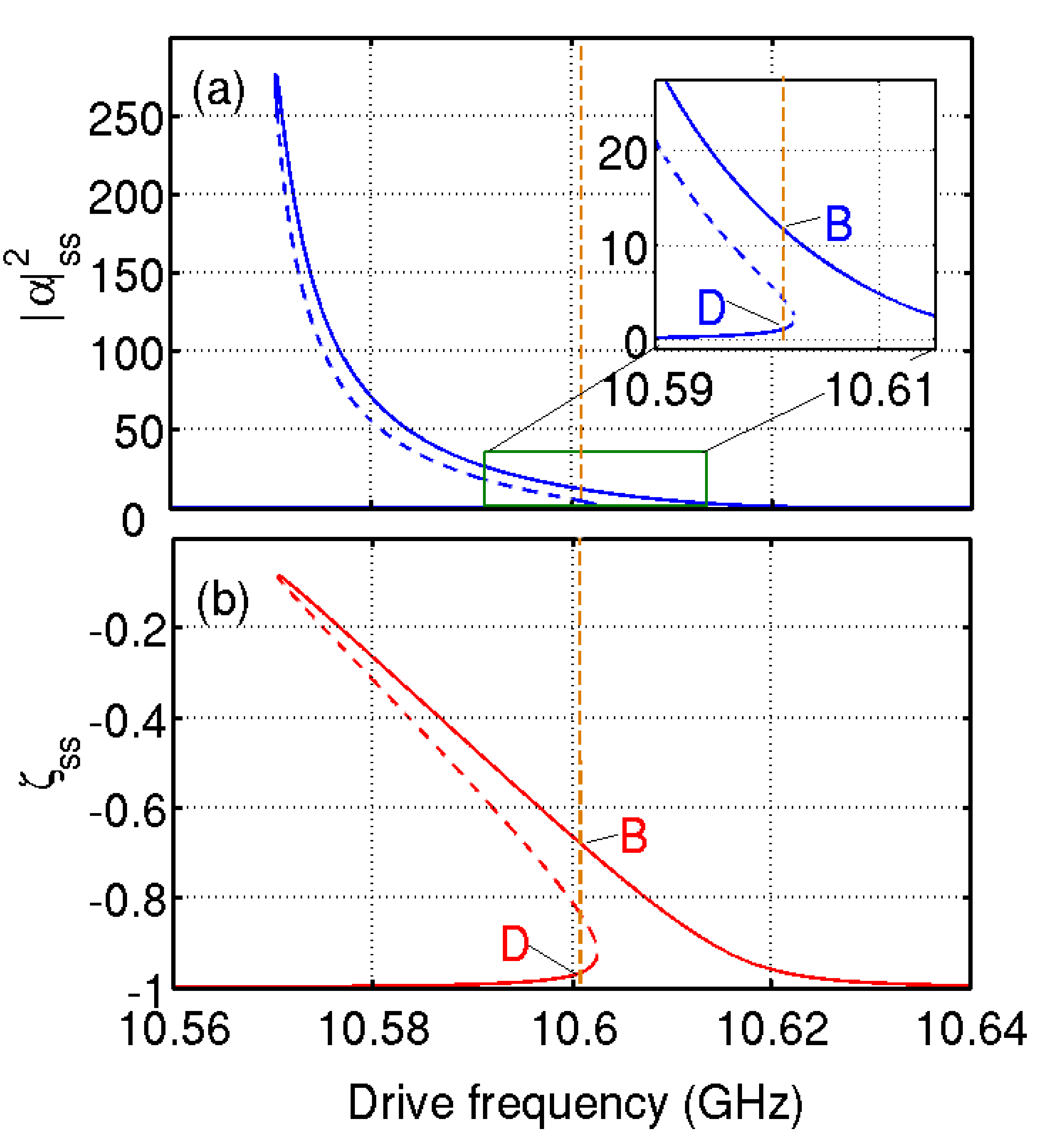
Figure 1: Maxwell-Bloch steady-state bistability of the JC oscillator in the dispersive regime WallsBook (2010) for the coupling strength to detuning ratio $g/\delta=0.14$, the drive amplitude to photon loss ratio $\varepsilon_{d}/(2\kappa)=25/3$ and the photon loss to spontaneous emission ratio $2\kappa/\gamma=12$. Here, ${\rm B(D)}$ denote the bright (dim) semiclassical states. (a) Intracavity field amplitude in the steady state (with the region of interest zoomed in the inset). (b) The corresponding atomic inversion $\zeta=\braket{\sigma_{z}}$. The broken orange line indicates the driving frequency at $10.6005\,$GHz, and the dashed lines in each curve depict the unstable branch.

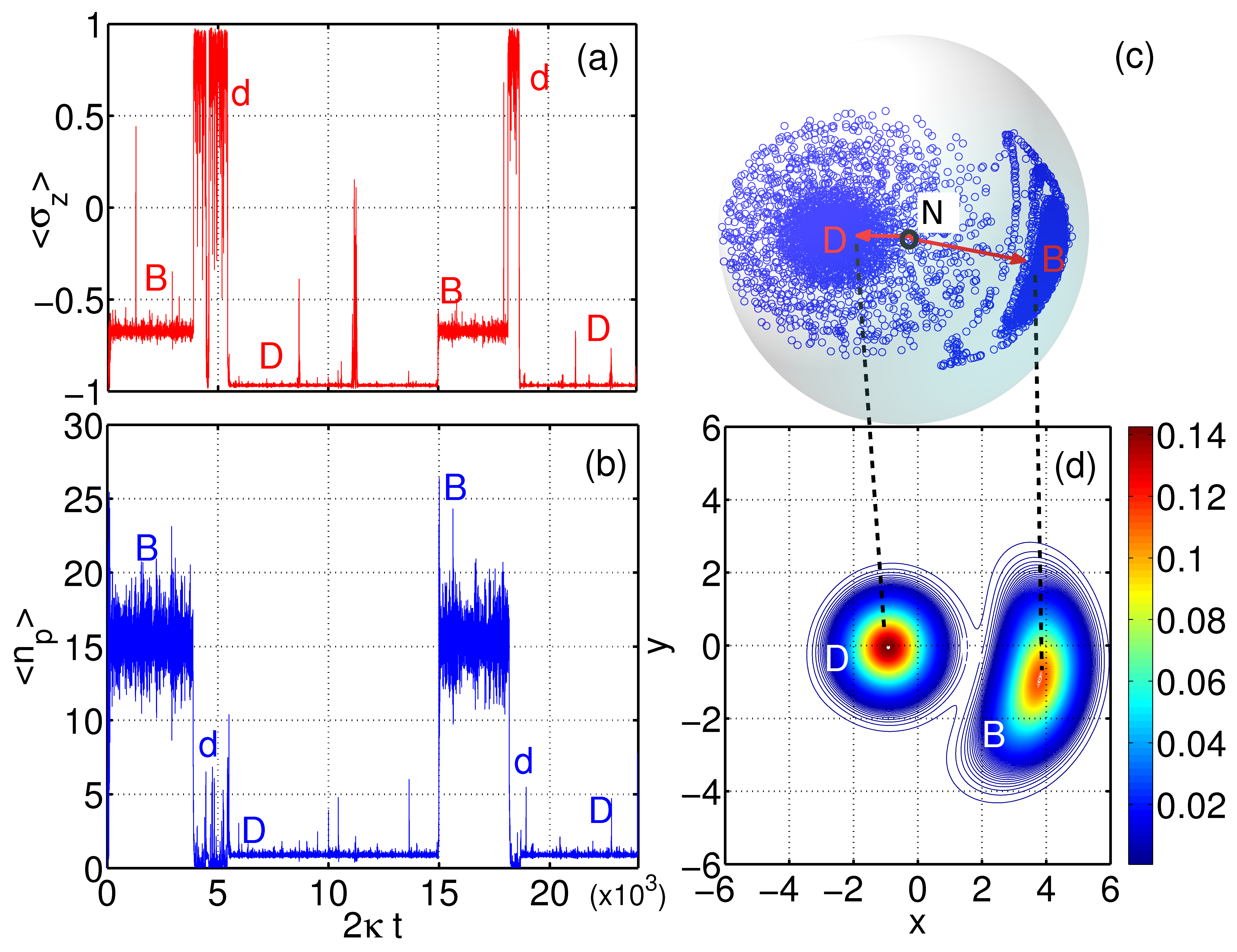
Figure 2: Quantum-activated simultaneous cavity and qubit switching illustrated using the JC model in the dispersive regime for $g/\delta=0.14$, $3\varepsilon_{d}/(2\kappa)=25$, $2\kappa/\gamma=12$ and $N_{\textrm{crit}}\simeq 13$. Here, ${\rm B(D)}$ denote the bright (dim) metastable states and ${\rm d}$ denotes the nonclassical dark state. (a) Atomic population inversion $\Braket{\sigma_{z}}$. (b) The accompanying intracavity photons $\Braket{n_{p}}=\Braket{a^{\dagger}a}$ as a function of the dimensionless time $2\kappa t$ for a single quantum trajectory. The trajectories in (a) and (b) depict simultaneous switching between the bright (B) and dim (D) states. (c) Illustration depicting the two metastable state distributions in the Bloch sphere (as viewed from the north pole indicated by the letter N). Data points corresponding to the dark state are omitted for clarity. The red arrows point to the two metastable states (B and D). (d) Contour plot of the joint quasidistribution function $Q(x+iy)$ for $f_{d}=\omega_{d}/2\pi=10.6005\,$ GHz, as indicated in Fig. 1, showing two peaks corresponding to two semicoherent states, indicating the presence of cavity bimodality.

In this paper, we demonstrate that in a nonlinear intermediate driving regime of circuit QED, the system dynamics exhibits a simultaneous bistability of the qubit and resonator. We support this claim both theoretically, with analytical and numerical results, as well as with experimental measurements obtained from a circuit QED device, consisting of a transmon qubit coupled to a 3D microwave cavity Paik (2011). In particular we report the following findings. (1) The switching process occurs simultaneously for the two coupled quantum oscillators. (2) The ensemble averaged amplitudes of both cavity and qubit exhibit a coherent partial cancellation. Such cancellation, predicted theoretically for a single nonlinear mode by Drummond and Walls in Drummond (1980), is here verified experimentally and shown to occur for both coupled oscillators. (3) The Duffing oscillator model with one quantum degree of freedom is not sufficient to account for the observed cavity nonlinearity when the two coupled quantum degrees of freedom are involved in the switching process. We also note that, the JC bistable semiclassical intracavity amplitude $|\alpha|_{\rm ss}^{2}$ (with $\alpha=\braket{a}$) in the steady state, plotted in Fig. 1(a), does not show any coherent cancellation feature, nor does the bistable average atomic inversion $\zeta_{\rm ss}=\braket{\sigma_{z}}_{\rm ss}$ shown in Fig. 1(b). Instead, both curves are skewed Lorentzians with the position of their peaks approaching the bare cavity frequency for increasing drive. By increasing the drive strength beyond what is shown in Fig. 1(a) one finds a critical point in the phase space between bistable and linear behavior, lying on the line where the frequency of the drive equals the bare cavity resonance frequency. Beyond that point, the system behaves as a linear oscillator, in contrast to the corresponding Duffing oscillator Bishop (2010), and exhibits no bistability.

II Theoretical models

In order to develop a comprehensive understanding of the system response, we will consider several different theoretical models: (i) multilevel transmon-cavity GJC model — the most complete in the context of superconducting devices; (ii) two-level ‘atom’-cavity JC model which is universal to many strong light-matter coupling scenarios, and (iii) a simplified dressed-cavity Duffing oscillator approximation. To complement the numerical simulations of the three models, we additionally compare the results for the cavity transmission with those coming from an analytical formula, obtained by modeling the transmon itself as a nonlinear oscillator.

We will now define the system Hamiltonians associated with models (i)-(iii). When one cavity field mode of frequency $\omega_{c}$ (with corresponding photon annihilation and creation operators $a$ and $a^{\dagger}$ respectively) is coupled to a multilevel system with unperturbed states $\Ket{n}$, the coherently-driven GJC Hamiltonian can be written as (setting $\hbar=1$) Koch (2007)

$$H_{\rm{GJC}}^{\text{(i)}}=\omega_{c}a^{\dagger}a+\sum_{n}\omega_{n}\Ket{n}\Bra{n}+\sum_{m,n}g_{mn}\Ket{m}\Bra{n}(a+a^{\dagger})\\ +i\varepsilon_{d}(a^{\dagger}e^{-i\omega_{d}t}-ae^{i\omega_{d}t}),$$ (1)

where $\varepsilon_{d}$ is the strength of a monochromatic external field with frequency $\omega_{d}$ driving the cavity mode. The sum in the third term describes the interaction and is customarily modified to $\sum_{m}g_{m,m+1}\left(\Ket{m}\Bra{m+1}a^{\dagger}+\textrm{h.c.}\right)$ in the rotating wave approximation (RWA). The interaction energies in the RWA have the approximate form $g_{mn}\approx g\sqrt{m+1}\,\,\delta_{m+1,n}$, with $g$ being the dipole coupling strength. Depending on the range of $n$ and the form of $\omega_{n}$ we can distinguish the two-level atom ($n=1$, $m=0$, $\omega_{n}=\omega_{q}$) – the JC model – from a transmon ($n=1,2,\ldots,N_{\textrm{max}}$, $\omega_{n}=\omega(n)$) – the GJC model. The JC model in the RWA reads

$$H_{\rm{JC}}^{\text{(ii)}}=\omega_{c}a^{\dagger}a+\frac{1}{2}\omega_{q}\sigma_{z}+g(a^{\dagger}\sigma_{-}+a\sigma_{+}),$$ (2)

with $\sigma_{\pm}$ the raising (lowering) pseudospin operators and $\sigma_{z}=2\sigma_{+}\sigma_{-}-1$ the inversion operator. In the presence of dissipation, the cavity mode is damped at a rate $2\kappa$ doublerate while spontaneous emission is present at a rate $\gamma$ for a qubit dephased at a rate $\gamma_{\phi}$.

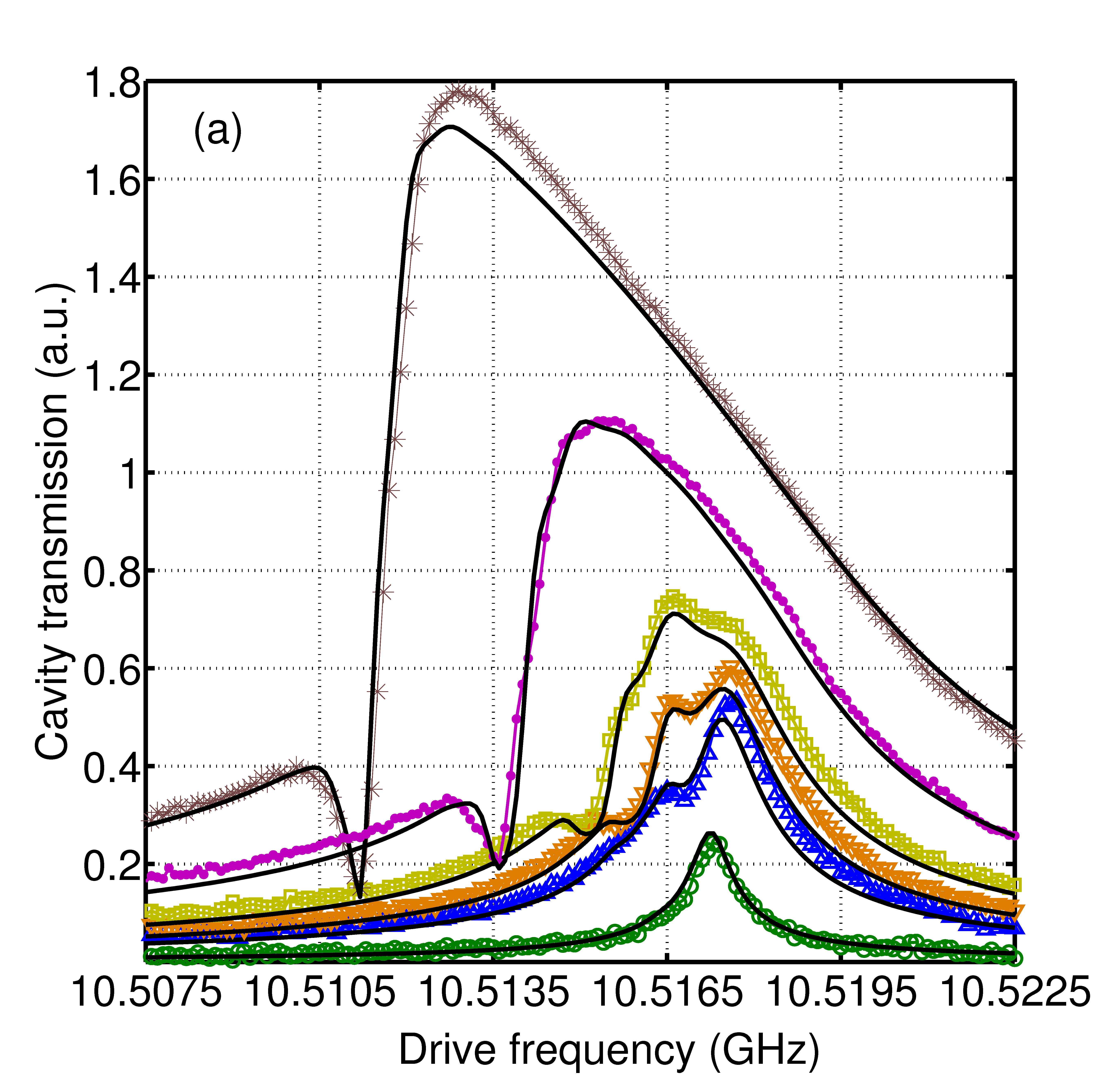
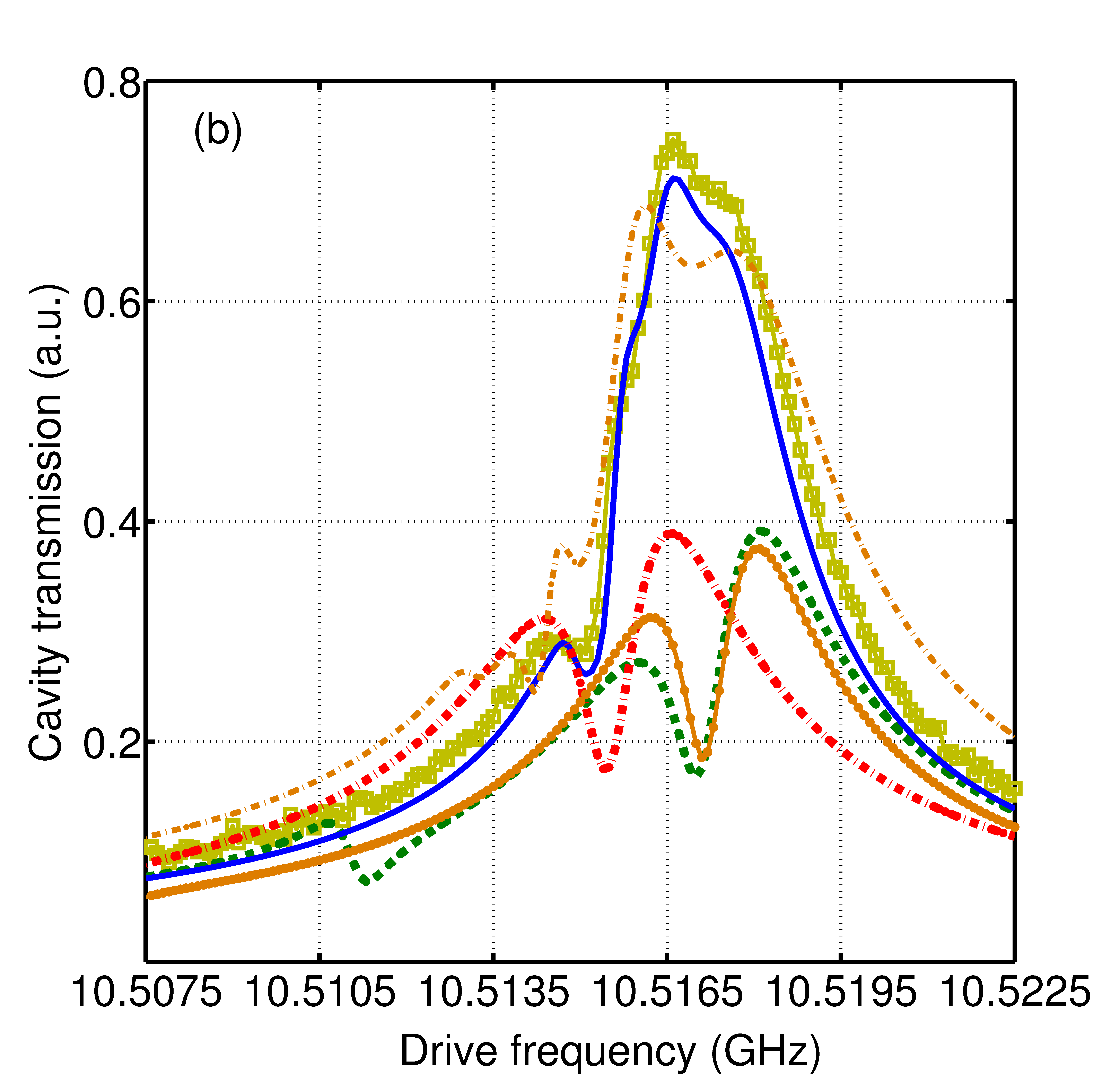
Figure 3: Theory and experiment showing the cavity nonlinearity for increasing drive strength. (a) The experimentally measured transmission amplitude (in patterned lines) of the device $D_{1}$, consisting of a cavity resonator with bare frequency $f_{c}=\omega_{c}/2\pi=10.426\,$GHz coupled to a transmon qubit with lower transition frequency $f_{q}=\omega_{q}/2\pi=9.442\,$GHz, for six increasing values of the driving strength ($-66\,$dBm: green $\circ$, $-52\,$dBm: blue $\triangle$, $-49\,$dBm: orange $\triangledown$, $-46\,$dBm: yellow $\square$, $-41\,$dBm: pink $\bullet$ and $-36\,$dBm: brown $\ast$) superimposed on top of the theoretical predictions of the GJC model with four levels (shown in solid black lines). (b) Cavity transmission as a function of the driving frequency for all the considered theoretical models: GJC in solid blue, JC in dashed green, its Duffing reduction in dot-dashed red and the effective Fokker-Planck model in orange with full circles for the experimental transmon anharmonicity coefficient $\chi/2\pi=-150\,$MHz, and a dot-dashed line for $\chi/2\pi=-20\,$MHz, alongside the experimental data in yellow $\square$ for the driving power of $-46\,$dBm. It is clear that (only) the GJC model shows excellent agreement with the experimental data.

It is possible to approximate the Hamiltonian of Eq. (2) further in the strongly dispersive regime, defined by the strong detuning $\delta=\left|\omega_{c}-\omega_{q}\right|\gg g$ between the two coupled oscillators. Under an appropriate decoupling transformation Carbonaro (1979); Peano (2010) $H_{\rm JC}$ can be recast in the form $H^{\prime}_{\rm JC}=\omega_{c}a^{\dagger}a+(1/2)(\omega_{c}-\Delta)\sigma_{z}$, involving the operator $\Delta=\sqrt{\delta^{2}+4g^{2}\mathcal{N}}$ where $\mathcal{N}=a^{\dagger}a+\sigma_{+}\sigma_{-}$ is the operator of the total number of excitations $N$. In the dispersive regime, provided that $N/N_{\rm crit}\ll 1$ ComparisonRD , we can expand up to the quartic order in the field variables. After normal ordering we obtain the following dressed-cavity Duffing oscillator Hamiltonian

$$H_{\text{D}}^{\text{(iii)}}=\left(\omega_{c}+\frac{g^{4}}{\delta^{3}}-\frac{g^{2}}{\delta}\sigma_{z}+2\frac{g^{4}}{\delta^{3}}\sigma_{z}\right)a^{\dagger}a+\frac{g^{4}}{\delta^{3}}\sigma_{z}{a^{\dagger}}^{2}a^{2},$$ (3)

where setting $\sigma_{z}=-1$ is a justifiable approximation for low enough driving amplitudes, yielding a bistable quantum Duffing oscillator driveterms . The third term in the parentheses is the leading-order term $\chi^{(0)}_{c}=(g^{2}/\delta)\sigma_{z}$ which is the familiar Stark shift Blais (2004) and provides a valuable tool for qubit readout (with $\left|\chi^{(0)}_{c}\right|\gg\kappa$). Here, in the bifurcating dispersive region we are studying, the following hierarchy of scales applies Bishop (2010): $\gamma,\gamma_{\phi}\ll 2\kappa\ll\varepsilon_{d}\lower 3.01385pt\hbox{$\;\stackrel{{\scriptstyle\textstyle<}}{{\sim}}\;$}g^{2}/\delta\ll g<\delta\ll\omega_{c}$. The intracavity excitation number is of the order of $N_{\rm crit}$, where this perturbation expansion is not strictly valid. However, as we will see later, it gives qualitatively meaningful results.

Having defined the different model Hamiltonians under consideration, we now evolve the corresponding master equations (MEs) in the finite Hilbert state basis numerically, starting from a Fock state of zero photons and the qubit in the ground state, until it reaches a steady state. Note that the steady state obtained is independent of the choice of the initial conditions.

III Activated dynamics in the dispersive regime

Driving the system beyond the low power regime has a profound effect on the response. We illustrate this fact in Fig. 2, where we depict the qubit inversion $\braket{\sigma_{z}}$ in Fig. 2(a), the photon cavity number $\braket{n_{p}}=\braket{a^{\dagger}a}$ in Fig. 2(b), alongside their associated cavity quasidistribution function in Fig. 2(d), employing the exact ME simulations [Fig. 2 (d)] and single quantum trajectories from the stochastic Schrödinger equations (SSE) using the second-order weak scheme in the diffusive approximation BreuerBook (2002); PlatenBook (1995) [Figs. 2(a) and 2(b)]. Single quantum trajectories, corresponding to the unravelling of the ME for the JC Hamiltonian, depict the switching between the two metastable semiclassical states as a result of quantum fluctuations. The switching occurs simultaneously for the qubit [Fig. 2(a)] and the cavity [Fig. 2(b)]. The corresponding photon histogram shows quasi-Poissonian statistics obeyed by the two metastable states, one with mean photon occupation of the order of $N_{\textrm{crit}}$ (called ‘bright’ state), one with mean occupation of about a photon (called ‘dim’ state) as well as the distribution of a nonclassical (called ‘dark’) state (for more details see the Supplementary Information). In Fig. 2(c) we draw a sketch illustrating the qubit distribution in the steady state, as viewed from the north pole of the Bloch sphere, for a single quantum trajectory. Red arrows point to the two semiclassical qubit states, corresponding to the two metastable quasicoherent cavity states [depicted by color contour plots in Fig. 2(d)] between which quantum-activated switching takes place. The $Q$ function plot in Fig 2(d) also shows the position in the phase space of the coherently cancelling states. The equal height of the $Q$ function peaks indicates the boundary of a first-order dissipative quantum phase transition Carmichael (2015); Protocol (2010). This transition is marked by the switching rates to the bright and to the dim state being of the same order of magnitude Carmichael (2015); DykmanSmelyanskii (1988). In our case, as well as in the exact photon statistics section of Drummond (1980), switching is induced by quantum fluctuations only, as the thermal bath to which the system is coupled is at zero temperature. The trajectories depicted for illustration in Fig. 2 evidence sudden simultaneous jumps. Bistability and synchronisation were studied for the two-level Rabi model in Zhirov (2008). Note that, in contrast to the cavity field and $\left|\Braket{\sigma_{-}}\right|$, the exact ME results for the photon number and $\Braket{\sigma_{z}}$ show no coherent cancellation in the steady-state response. The mean-field behavior, depicted in Fig. 1, shows further that the coherent cancellation is purely a quantum effect at zero temperature, occurring when forming the ensemble averaged quantities, and is already present in the most approximate dressed-cavity Duffing model, even if the qubit is unmonitored.

IV The nonlinear resonator transmission lineshape

In Fig. 3(a) we compare theoretical and experimental transmission amplitudes of a 3D cavity with embedded transmon (device $D_{1}$, details in the Supplementary Information) for different driving strengths. We observe that, as the driving power is increased, the experimental cavity lineshape develops nonlinear features and a coherent cancellation dip appears. We find perfect agreement with the GJC model. In Fig. 3(b) we show the cavity transmission for the intermediate drive power of $-46\,$ dBm for all the models discussed. We observe that the JC model predicts the split of the main peak at the correct position, as opposed to its Duffing reduction, yet fails to capture the position of the dip emerging at a lower frequency. The GJC model with four transmon levels can resolve all the details necessary for a quantitative comparison and provides indeed the most complete description of the cavity nonlinearity.

The behavior of the GJC oscillator depends strongly on the drive strength and frequency, and their relation to the coupling and dissipation rates CarmichaelBook (2008); Bishop (2010). We find theoretically that the coherent cancellation dip in transmission, discovered by Drummond and Walls for the Duffing oscillator Drummond (1980), appears in the dispersive response of both the cavity and the qubit within the full nonlinearity of the JC model, where the departure from the mean-field predictions is appreciable and the Duffing oscillator approximation is no longer valid. For the Duffing oscillator the dip is present in the first moment of the field operator, $\left|\braket{a}\right|$, calculated using the generalized $P$ representation Drummond (1980). It is purely a phase effect as the dip does not appear in the number of intracavity photons in the steady state $\Braket{n_{\textrm{p}}}=\Braket{a^{\dagger}a}$. The coherent cancellation dip appears as well in the qubit projection $\left|\braket{\sigma_{-}}\right|$ (see the Supplementary Information for more details). The presence of this dip in the cavity response has also been observed in our experimental measurements, which depict the development of nonlinearity for increasing drive strengths within the region of bistability. Similar cancellation effects appear also in classical dissipative systems out of equilibrium, in the presence of thermal fluctuations Drummond (1980). The observed dip, appearing progressively in a measurement of complex amplitude, is due to the phase differences between the two metastable states. In the experimental response we can also discern a split of the main peak, alluding to dynamical Rabi splitting Bishop (2009). The position of the dip shifts to the lower frequencies with increasing drive strength, while the split gradually fades away in favour of a Duffing-type profile.

In order to gain a further insight, we undertake an analytical approach by identifying an effective Hamiltonian to produce a (second-order) Fokker-Planck equation (FPE) for the transmon, following the adiabatic elimination of the cavity. FPEs in the generalized $P$ representation can be used to solve exactly for the steady state of quantum systems subject to the so-called ‘potential conditions’, and have been used to study single nonlinear resonator systems WallsBook (2010). For our two-oscillator model, these conditions are not satisfied, yet in the limit $2\kappa\gg\gamma,\gamma_{\phi}$ the cavity can be eliminated in a similar fashion to the method of Drummond (1981). This process leaves a FPE for an effective one-oscillator system, which resembles a driven, damped quantum Duffing oscillator with anharmonicity $\chi$ Drummond (1980) but with parameters that are nontrivial functions of those of the full system. Full details of this method can be found in Elliott (2016). The first moment of the cavity field in the steady state is

$$\langle a\rangle=\frac{2}{\tilde{\gamma}_{c}}\left[\varepsilon_{d}-\frac{\tilde{\varepsilon}g}{\chi c}\frac{~{}_{0}{F}{{}_{2}}\left(c+1,c^{*};2\left|\displaystyle\frac{\tilde{\varepsilon}}{\chi}\right|^{2}\right)}{~{}_{0}{F}{{}_{2}}\left(c,c^{*};2\left|\displaystyle\frac{\tilde{\varepsilon}}{\chi}\right|^{2}\right)}\right],$$ (4)

where $~{}_{0}{F}{{}_{2}}(x,y;z)$ is a generalized hypergeometric function, and we have defined effective decay constants for the cavity $\tilde{\gamma}_{c}=\kappa+2i\Delta\omega_{c}$ and transmon $\tilde{\gamma}_{q}=\gamma+2i\Delta\omega_{q}+2g^{2}/\tilde{\gamma}_{c}$ respectively (with $\Delta\omega_{c(q)}=\omega_{c(q)}-\omega_{d}$), effective drive strength $\tilde{\varepsilon}=-2ig\varepsilon_{d}/\tilde{\gamma}_{c}$ and also $c=\tilde{\gamma}_{q}/(2i\chi)$. The calculated transmission amplitude via Eq. 4 is plotted in Fig. 3(b) and compared to the exact ME results alongside the experimental data. The effective Fokker-Planck model exaggerates the actual nonlinearity in this regime, yet a lower value of $\chi$ allows us to capture the essential features of the full transmon-cavity-driven interaction (more details in the Supplementary Information).

V Discussion and concluding remarks

We have examined the dispersive interaction of a single qubit and a microwave cavity mode, tracking nonlinearity with increasing drive power. When the regime of bistability is reached, simultaneous switching events allow for both of the metastable states to participate even at zero temperature. Their different phases cause the ‘dip’ in coherent transmission, for which we have presented theoretical and experimental evidence. Interestingly, the dim quasicoherent state is preceded by a lower amplitude nonclassical state which is not predicted by the mean-field treatment. This state is characterized by very low photon numbers and intense fluctuations in the qubit inversion, which occupies now the north pole of the Bloch sphere. For high excitations, beyond the Duffing oscillator regime, both the cavity and the qubit participate in the switching, and the quantitative comparison with the experiment necessitates the inclusion of more than two levels of the transmon. The superconducting devices we have considered serve as examples of quantum activation with more than one quantum oscillator.

The data underlying this work is available without restriction SurreyDep .

Acknowledgements Th. K. M. wishes to thank H. J. Carmichael and L. Riches for instructive discussions. Th. K. M. and M. H. S. acknowledge support from the Engineering and Physical Sciences Research Council (EPSRC) under grants EP/I028900/2 and EP/K003623/2. E. G. acknowledges support from the EPSRC under grant EP/L026082/1. P. J. L. acknowledges support from the EPSRC under grants EP/J001821/1 and EP/M013243/1.

$\star\star\star\star\star$

SUPPLEMENTARY INFORMATION

VI Experimental setup

Our devices consist of single-junction transmon qubits embedded in aluminium 3D cavities thermally anchored at $10\,$mK in a dilution refrigerator. We have measured two different devices, referred to as $D_{1}$ and $D_{2}$, whose characteristic parameters can be found in Table 1. Fig. 4(a) shows the device $D_{1}$ consisting of a two-ports Al microwave cavity which holds a lithographically patterned Al transmon qubit [Fig. 4(b)] on a sapphire substrate. The Josephson junction was fabricated using a double-angle shadow evaporation technique. Fig. 4(c) shows the experimental setup used for measuring $D_{1}$, a similar setup was used for $D_{2}$. For the device $D_{1}$ $(D_{2})$ we measured the transmitted (reflected) signal over many experiments using a heterodyne detection scheme and computed the average signal.

Each cavity has a bare resonant frequency of $f_{c}=\omega_{c}/(2\pi)$ supporting a mode coupled to a transmon with the lowest transition frequency $f_{q}\equiv f_{01}=\omega_{01}/(2\pi)$. The interaction between the uncoupled qubit state $\Ket{n}$ and the cavity with coupling strength $g$ causes a dispersive shift of the cavity resonance $f_{c}$, depending on the state of the qubit.

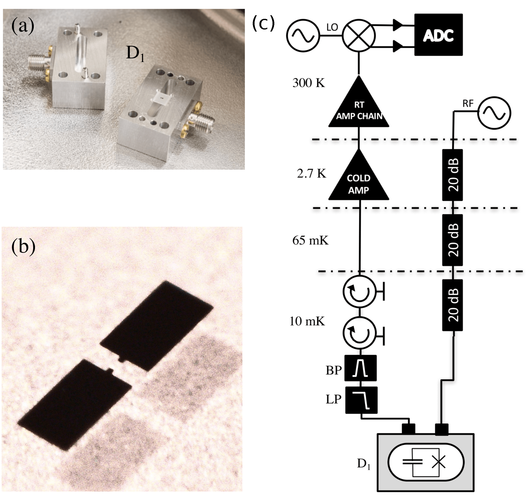
Figure 4: (a) The cross-section of device $D_{1}$: a two-ports Al microwave cavity, which holds a lithographically patterned Al transmon qubit on a sapphire substrate. The cavity is placed inside a magnetic shield at base temperature. (b) A picture of the transmon qubit consisting of two Al (a) pads of dimensions $350\,\mu$m by $450\,\mu$m connected by an Al/AlOx/Al Josephson junction. (c) The experimental setups used to measure the transmitted signal for the device $D_{1}$. An input microwave signal (RF) is sent to the sample through a highly attenuated microwave line. The output signal is first amplified by a cold amplifier and then by a series of room temperature amplifiers before being demodulated and recorded by an analog to digital converter (ADC). A bandpass filter (BP), a low pass filter (LP) and two circulators are used to prevent thermal and amplifier noise from reaching the sample.

Device	$f_{c}$ (GHz)	$\delta/2\pi$ (GHz)	$g/2\pi$ (GHz)	$E_{J}/E_{C}$	$T_{1}$ ($\mu$s)	$T_{2}$ ($\mu$s)
$D_{1}$	10.426	0.984	0.313	314	2.64	4.00
$D_{2}$	10.567	2.383	0.335	165	2.20	2.10

Table 1: Characteristic parameters of the experimental devices: $f_{c}$ is the bare cavity frequency, $\delta$ is the qubit-cavity detuning, $g$ is the coupling strength, $E_{J}/E_{C}$ is the ratio of the Josephson energy to the charging energy, $T_{1}$ is the relaxation and $T_{2}$ the dephasing time of the qubits.

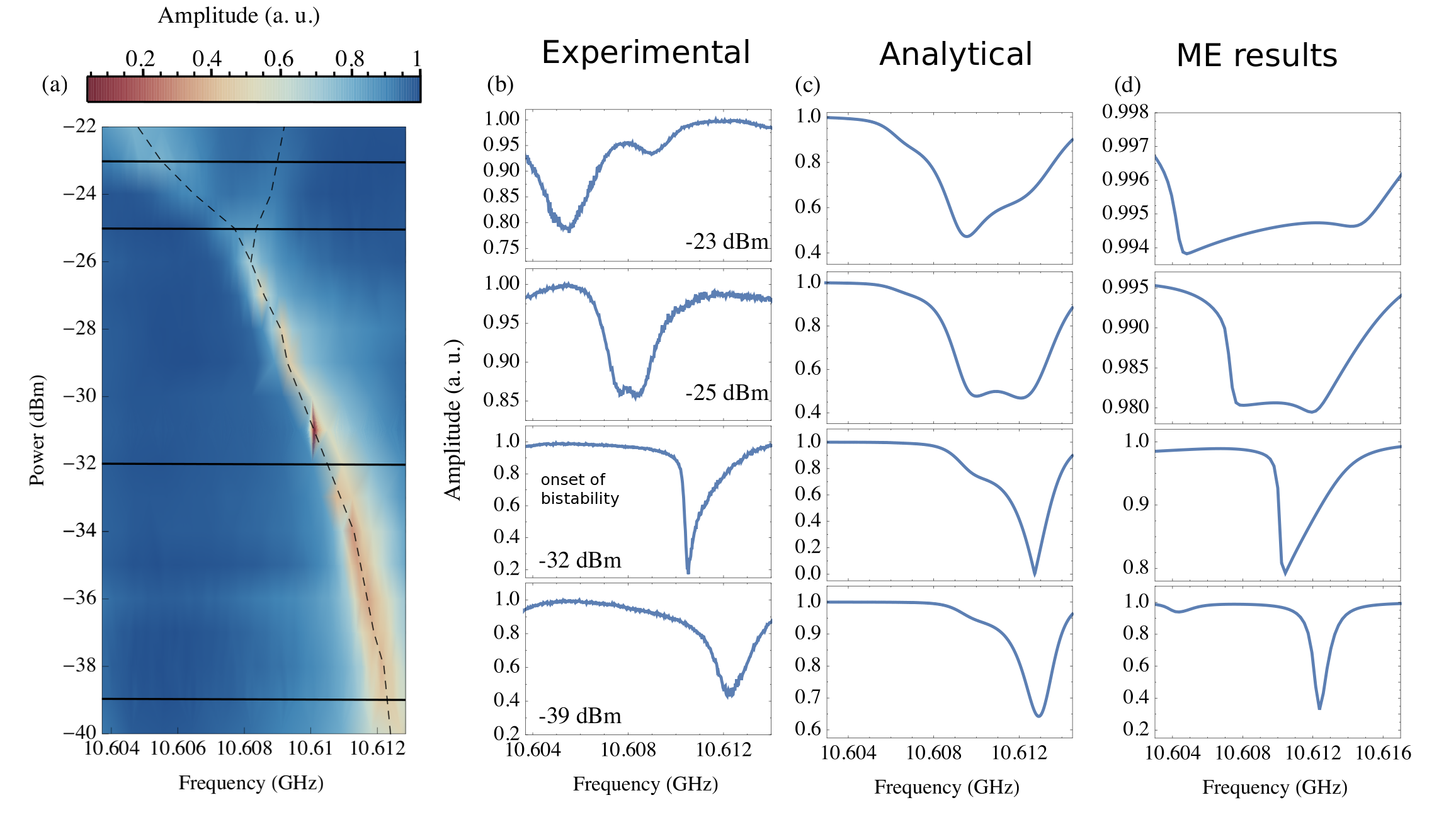
Figure 5: Experimental and theoretical reflection curves for the ground state excitation of the device $D_{2}$, consisting of a 3D cavity resonator coupled to a transmon qubit. The low power curves show a dispersive shift of $\chi^{(0)}_{c}=g^{2}/\delta$ from the bare cavity frequency. (a) Experimental reflection amplitude as a function of the drive frequency and power. At low driving power the response of the cavity is a Lorentzian centered at $10.612\,$GHz; as the power increases the Lorentzian minimum moves towards lower frequencies. Distortion of the Lorentzian shape occurs as the power is further increased as a result of bistability. At the power of $-32\,$dBm we mark the onset of bistability corresponding to the distorted Lorentzian shape with an abrupt wall-like profile. At a power of $-25\,$dBm we observe the emergence of two reflection features whose separation increases with increasing driving power. (b) Horizontal cuts through (a) at different drive powers ($-23\,$dBm, $-25\,$dBm, $-32\,$dBm, $-39\,$dBm). (c) Analytical results from the effective Fokker-Planck model. (d) ME simulations for a ten-level transmon with anharmonicity coefficient $\chi/2\pi=-242\,$MHz and dipole coupling strength $g/2\pi=335\,$ MHz.

In Fig. 5 we show the experimental reflection amplitude for a different device ($D_{2}$, see Table 1 for more details), as a function of the driving parameters, next to our theoretical predictions. The experimental Lorentzian curve [Figs. 5(a, b)] shifts towards lower frequencies with increasing power, followed by the emergence of a dip separation, in close agreement with the theoretical predictions shown in Figs. 5(c, d). The horizontal line at $-32\,$dBm marks the onset of bistability, corresponding to a frequency shift of $\kappa$. The analytical formulation already captures the pair of emerging dip lines occurring for increasing drive strength, in close agreement with the experiment. The ME results show more conspicuously the shift of the resonance curve to the left for lower drive strengths, but lead to a weaker separation because of thermal broadening.

VII Theoretical Remarks

VII.1 Formulation of the Master Equation

The master equation (ME) corresponding to the open driven GJC model consisting of a multilevel system (transmon qubit) coupled to a single cavity mode with resonance frequency $\omega_{c}$ reads

$$\dot{\rho}=-i[H_{\textrm{GJC}},\rho]+\kappa[\overline{n}(\omega_{c})+1]\mathcal{L}\{a,\rho\}+\kappa\overline{n}(\omega_{c})\mathcal{L}\{a^{\dagger},\rho\}+$$ (5)

$$+(\gamma/2)\mathcal{L}\left\{\sum_{j}\alpha_{j}\Ket{j}\Bra{j+1},\rho\right\}+$$

$$+(\gamma_{\phi}/2)\mathcal{L}\left\{\sum_{j}\beta_{j}\ket{j}\bra{j},\rho\right\},$$

where $\mathcal{L}\{A,\rho\}=2A\rho A^{\dagger}-A^{\dagger}A\rho-\rho A^{\dagger}A$ is the Liouvillian super-operator acting upon the Lindblad operator $A$, $\rho$ is the reduced density operator for the cavity-atom system, $2\kappa$ the cavity relaxation rate, $\gamma$ ($\gamma_{\phi}$) the transmon qubit dissipation (dephasing) rate and $\overline{n}(\omega_{c})=[e^{\omega_{c}/T}-1]^{-1}$ is the mean photon number for an oscillator with frequency $\omega_{c}$ at temperature $T$ ($k_{B}=1$) (we assume no thermal occupation for the transmon qubit). Expressions for the terms $\alpha_{j}$ and $\beta_{j}$ can be found in Bishop (2009).

The Hamiltonian $H_{\textrm{JC}}$ of the main text can also be inserted as the system Hamiltonian in (5), where customarily one uses pseudospin operators ($\sigma_{\pm},\sigma_{z}$) to account for the two-level system. The dressed-cavity system Hamiltonian in the Duffing approximation of the JC model, on the other hand, deserves special attention because the generator of the decoupling transformation required to decouple cavity and qubit does not commute with the drive term and the super-operators transform non trivially. As discussed in the main text, this approximation reads

$$H_{\textrm{D}}=[\omega_{c}+g^{4}/\delta^{3}-(g^{2}/\delta)\sigma_{z}+2(g^{4}/\delta^{3})\sigma_{z}+$$ (6)

$$+\mathcal{O}\left(g^{6}/\delta^{5}\right)]a^{\dagger}a+\left[g^{4}/\delta^{3}+\mathcal{O}\left(g^{6}/\delta^{5}\right)\right]\sigma_{z}{a^{\dagger}}^{2}a^{2}.$$

The above operator may be inserted in (5) for $\sigma_{z}=-1$ together with a drive term only to the leading order in $g/\delta$ and $N^{-1/2}$ Bishop (2010).

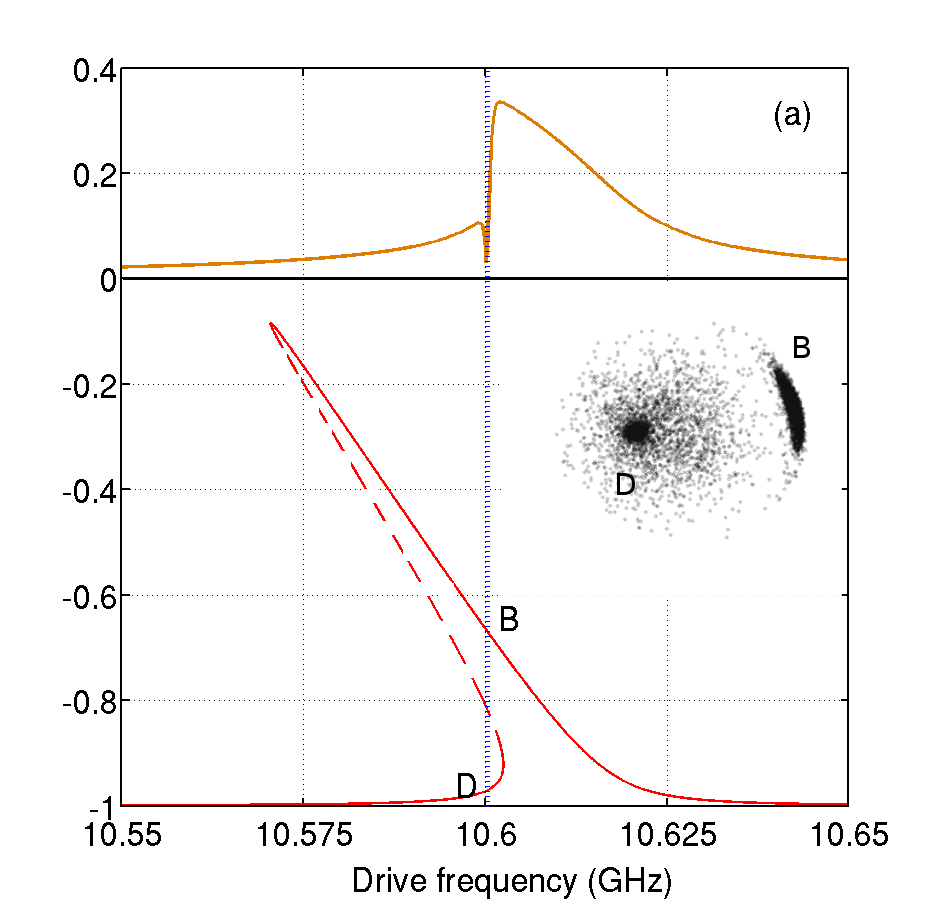
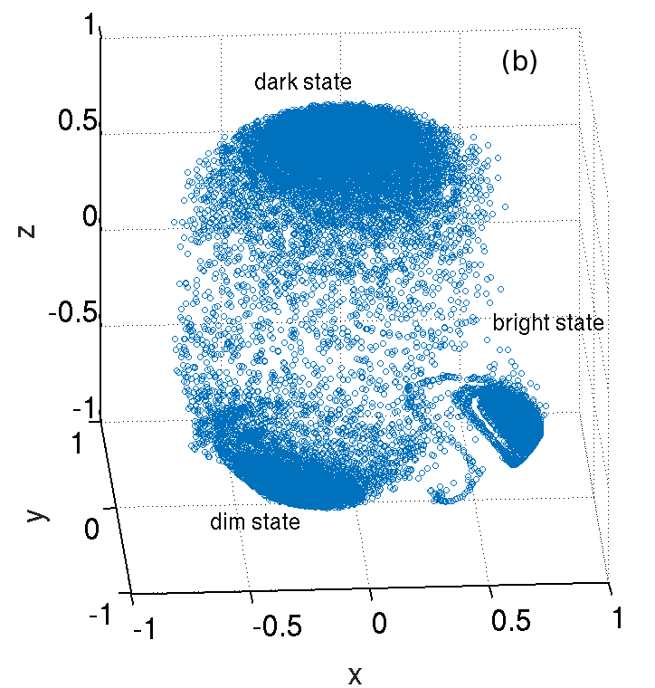
Figure 6: Qubit response in the JC model: (a) The steady-state solution of the Maxwell-Bloch equations for $\braket{\sigma_{z}}$ (lower panel) together with the pseudospin projection $\left|\braket{\sigma_{-}}\right|$ (upper panel) from the full ME solution, showing the coherent cancellation dip. The inset shows the equatorial plane view of the qubit vector from the north pole of the Bloch sphere, with the two distinct distributions corresponding to the states B and D. The broken line indicates the driving frequency $\omega_{d}/2\pi=10.6005\,$GHz. (b) The accompanying scatter-plot of the average Bloch vector (for $\omega_{d}/2\pi=10.6005\,$GHz) at different times for a single quantum trajectory calculated from the reduced qubit density matrix.

VII.2 Excitations in the JC oscillator

We will now focus on the behavior of the qubit during the bistable switching. In Fig 6(a) we depict the qubit response in the driving regime where the Duffing approximation is not applicable. As mentioned in the main text, we can observe that $\left|\braket{\sigma_{-}}\right|$ exhibits the characteristic coherent cancellation dip. In Fig. 6(b) we present the full scatter-plot for the qubit vector in the Bloch sphere, corresponding to the illustration of Fig. 2(c) (but now including the data for the dark state). In the inset of Fig. 7 we show one of the two components (the cavity field) of the system total excitation, the eigenvalue of the operator $\mathcal{N}$ for the JC oscillator. None of the constituents of $\mathcal{N}$ ($n_{p}$ and $\sigma_{+}\sigma_{-}$) show the coherent cancellation dip that characterizes the corresponding complex amplitude. Instead, they both present a distorted Lorentzian profile, which marks the onset of amplitude bistability.

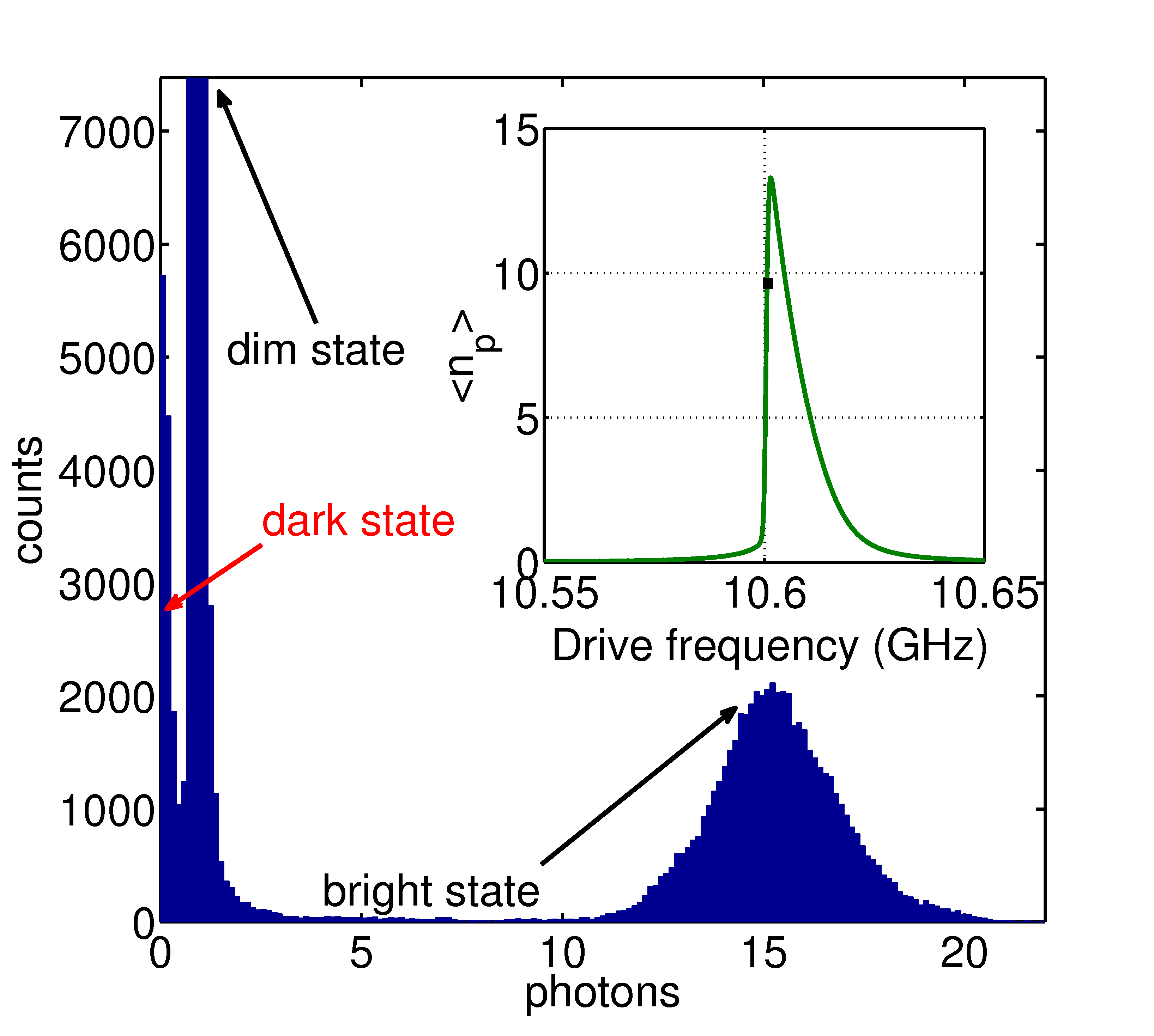
Figure 7: Photon histogram corresponding to the quantum trajectory of Fig. 2(b). The inset depicts $\braket{n_{p}}=\braket{a^{\dagger}a}$ as a function of the drive frequency for the same parameters used in Fig. 2. The point on the curve marks the coordinates corresponding to the response depicted in Fig. 2.

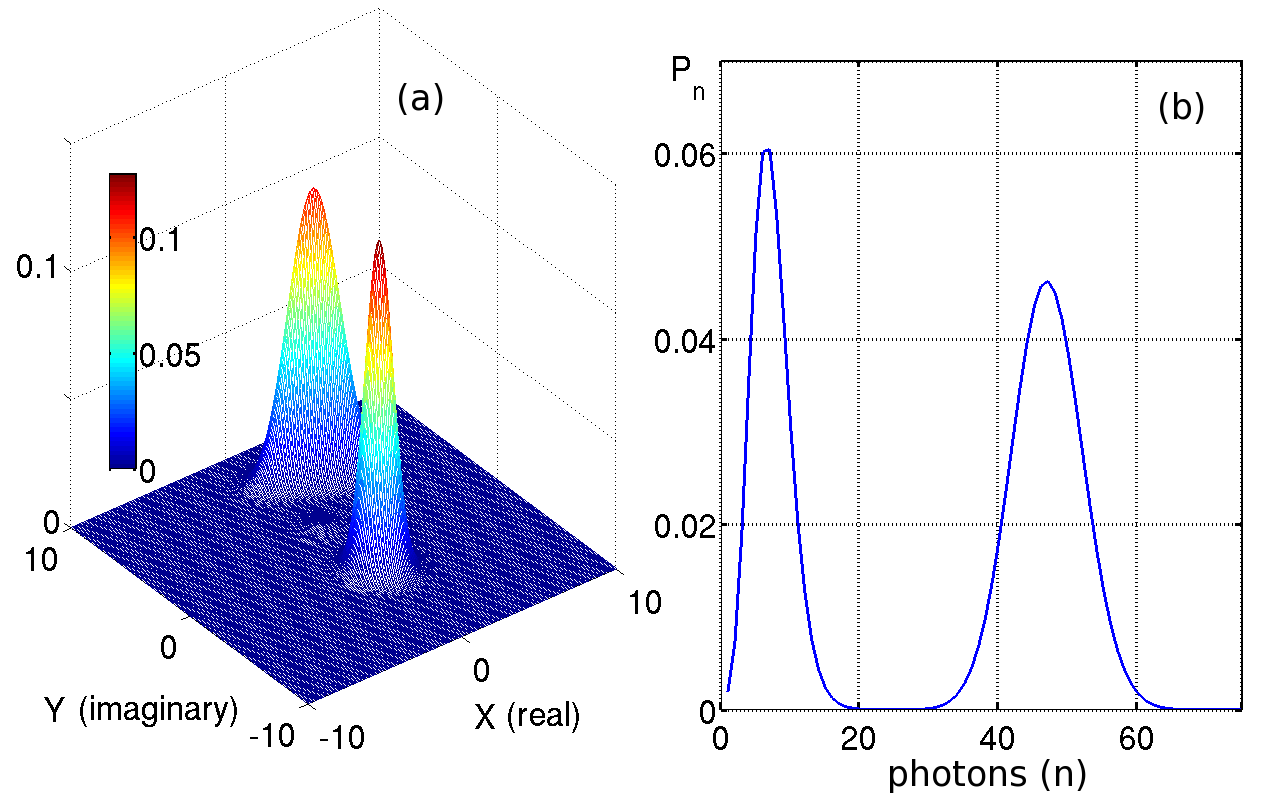
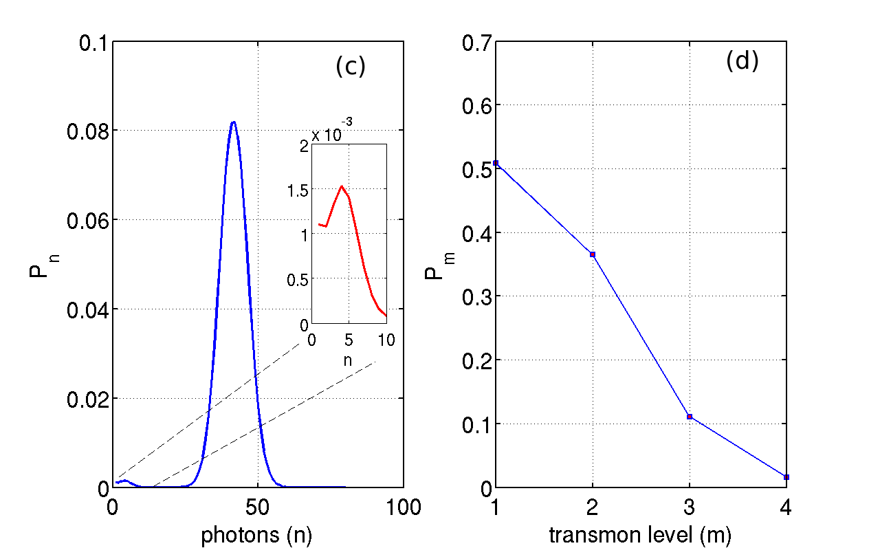
Figure 8: (a) $Q$ function and (b) $P_{n}$ distribution for a four-level transmon coupled to a cavity driven at a frequency $f_{d}=\omega_{d}/2\pi=10.6082\,$GHz prior to the coherent cancellation dip. (c) Probability distribution for the cavity occupancy, and (d) for the transmon, at the drive frequency $f_{d}=\omega_{d}/2\pi=10.6091\,$GHz past the position of the coherent cancellation dip.

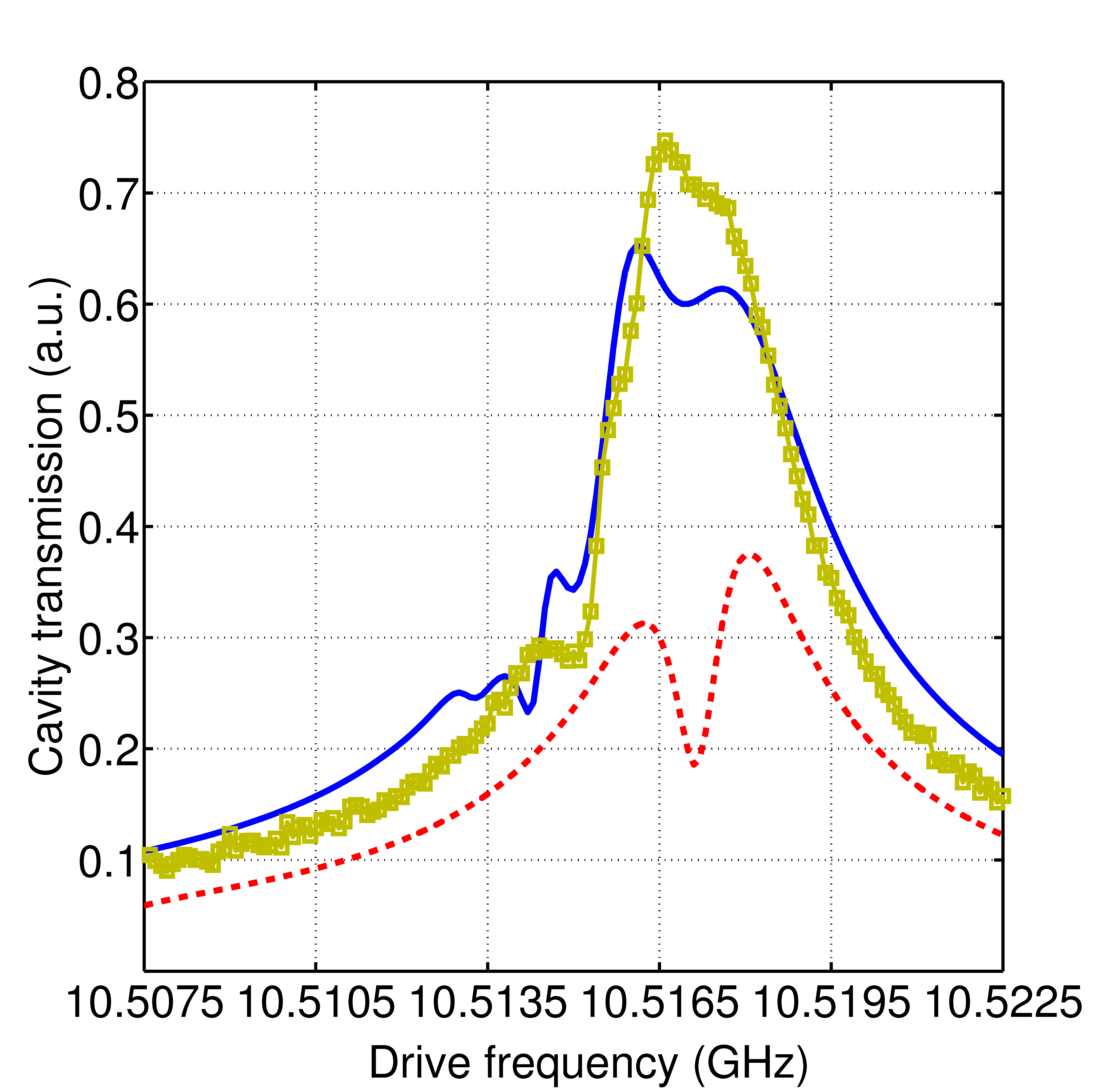
Figure 9: Cavity transmission as a function of the drive frequency for the effective Fokker-Planck model. The experimental data for the driving power of $-46\,$dBm are compared to the predictions of Eq. (4) for $\chi/2\pi=-150\,$MHz (dashed red line) and $\chi/2\pi=-20\,$MHz (solid blue line).

VII.3 Bimodality in the GJC

Bimodality is the underlying feature shaping the homodyne cavity response in the driving regime we have considered in the main text for the JC oscillator and its Duffing reduction. We show here that cavity bimodality is also present for a 4-level transmon, as indicated by the bimodal distribution in Fig. 8(a). The emergence of bimodality can be also traced in the transmon level occupation depicted in Fig. 8(b). The ‘dark’ state is indicated by the departure from the ‘dim’ state Poissonian distribution at $P_{0}$ [inset of Fig. 8(c)].

VII.4 Approaches to single-atom bistability

Single-atom absorptive bistability was first reported at resonance in Savage (1988), where two distinct states were identified that are long-lived in terms of the characteristic decay times of the two-level atom and cavity. Adiabatic elimination of the atomic variables has been used in Bonifacio to extract approximate Gaussian distributions able to adequately calculate mean square photon fluctuations for absorptive optical bistability at resonance. However, adiabatic elimination underestimates the dynamical rôle of the qubit in shaping the system response. There has been evidence that the effect of the qubit on the cavity mode is significant in a situation, where the drive is constantly tuned to maintain resonance Murch (2012). The two degrees of freedom describing the system and the inherent square root nonlinearity mark the departure from the Duffing oscillator Bishop (2010). Even in the dressed model describing dynamic Rabi splitting for the driven JC oscillator CarmichaelBook (2008), with one degree of freedom, the effective Hamiltonian leads to an equivalent description for the master equation of resonance fluorescence which, as is well known, cannot be reduced to a Fokker-Planck equation (FPE) CarmichaelBook1 following the adiabatic elimination used in Ref. Bonifacio .

VII.5 The effective Fokker-Planck model

We will now provide more details for the adiabatic elimination of the cavity in the transmon-cavity system. In this model we approximate the level structure of the transmon itself by a Duffing oscillator. We set $\omega_{n}=\omega_{q}n-\chi n(1-n)/2$ in Eq. (1), which is valid when the transmon occupation is relatively low. This Duffing approximation is a consequence of retaining the lowest order terms in the expansion of the Josephson potential Koch (2007). We then adiabatically eliminate the cavity from the system in the limit $2\kappa\gg\gamma$, and solve the Fokker-Planck equation analytically for the steady-state distribution. The solution obtained retains much of the structure of the full system despite the elimination process, and also allows us to recover the moments of the cavity field in the steady state. Thus, we model the transmon-cavity system as a nonlinear oscillator, with the first moment given by the result in Eq. (4).

We can also use the intracavity amplitude to plot the reflection of the cavity. In Fig. 5(c) we show the calculated reflection for the device $D_{2}$, compared with experimental results. For a further comparison we solve numerically the corresponding ME for the same parameters, and account for a finite temperature $T\simeq 200\,$mK in the presence of dissipation. For this device we see that the features of the analytical reflection spectra agree qualitatively with both experiment and ME at all four plotted powers.

For the device $D_{1}$, this analytical solution does not provide a good fit to the experimental data, since we are no longer operating in the limit $2\kappa\gg\gamma$. When $\kappa\approx\gamma$, this solution appears to overestimate the effect of the transmon nonlinearity on the cavity transmission spectrum. In Fig. 9 we plot the cavity amplitude for different values of the anharmonicity coefficient, comparing with the experimental data. We see that for the true device anharmonicity of $\chi/2\pi=-150\,$MHz the response resembles the JC oscillator in Fig. 3(b). If a much lower anharmonicity coefficient $\chi/2\pi=-20\,$MHz is selected, then the response is in closer agreement with the GJC model and experiment. This is consistent with the idea that the nonlinearity is overestimated in this approximation – if the experimental nonlinearity happens to be large it is then additionally magnified by the approximation so that the transmon behaves like a true two-level system. The solution to make the model useful in this regime is to choose an effective anharmonicity parameter $\chi$ smaller then the one measured by the experiment, so that it is enhanced to the level of the true experimental value by the approximation.

$\star\star\star\star\star$

References

- Haroche (2001) J. Raimond, M. Brune and S. Haroche, Rev. Mod. Phys. 73, 565 (2001).
- Koch (2007) J. Koch et al., Phys. Rev. A 76, 042319 (2007).
- Chiorescu (2004) I. Chiorescu et al., Nature (London) 431, 159 (2004).
- Wallraff (2004) A. Wallraff, et al., Nature (London) 431, 162 (2004).
- Nakamura (1999) Y. Nakamura, Y. A. Pashkin and J. S. Tsai Nature (London) 398, 786 (1999).
- WallsBook (2010) D. F. Walls and G. J. Milburn, Quantum Optics (Springer, Berlin, 2010).
- Aspelmeyer (2014) M. Aspelmeyer, T. J. Kippenberg and F. Marquardt, Rev. Mod. Phys. 86, 1391 (2014).
- Carmichael (2015) H. J. Carmichael, Phys. Rev. X 5, 031028 (2015).
- Rempe (1991) G. Rempe et al., Phys. Rev. Lett. 67, 1727 (1991).
- Kerckhoff (2011) J. Kerckhoff, M. A. Armen and H. Mabuchi, Opt. Express 19, 24468 (2011).
- Tian (1992) L. Tian and H. J. Carmichael, Phys. Rev. A 46, R6801(R) (1992).
- Bishop (2009) L. S. Bishop et al., Nat. Phys. 5, 105 (2009).
- JBA (2009) R. Vijay, M. H. Devoret and I. Siddiqi, Rev. Sci. Instrum. 80, 111101 (2009).
- CarmichaelBook (2008) H. J. Carmnichael, Statistical Methods in Quantum Optics 2 (Springer, 2008).
- Murch (2012) K. W. Murch et al., Phys. Rev. B 86, 220503(R) (2012).
- Boissonneault (2010) M. Boissonneault, J. M. Gambetta and A. Blais, Phys. Rev. Lett. 105, 100504 (2010).
- Bishop (2010) L. S. Bishop, E. Ginossar and S. M. Girvin, Phys. Rev. Lett. 105, 100505 (2010).
- Reed (2010) M. D. Reed et al., Phys. Rev. Lett. 105, 173601 (2010).
- DykmanSmelyanskii (1988) M. Dykman and V. N. Smelyanskii, Sov. Phys. JETP 67, 1769 (1988).
- DykmanBook (2012) M. I. Dykman, Fluctuating Nonlinear Oscillators (Oxford University Press, 2012).
- Peano (2010) V. Peano and M. Thorwart, Europhys. Lett. 89, 17008 (2010).
- Kamenev (2011) A Kamenev, Field Theory of Non-equilibrium Systems (Cambridge University Press, Cambridge, UK 2011).
- Maier (1992) R. S. Maier and D. L. Stein, Phys. Rev. Lett. 69, 3691 (1992).
- Dykman (1994) M. I. Dykman, M. M. Millonas and V. N. Smelyanskiy, Phys. Lett. A 195, 53 (1994).
- Graham (1984) R. Graham and T. Tél, Phys. Rev. Lett. 52, 9 (1984).
- Paik (2011) H. Paik et al., Phys. Rev. Lett. 107, 240501 (2011).
- Drummond (1980) P. D. Drummond and D. F. Walls, J. Phys. A 13, 725 (1980).
- (28) Here we denote the photon loss rate by , in alignment with the rate equations of laser theory.
- Carbonaro (1979) P. Carbonaro, G. Compagno and F. Persico, Phys. Lett. 73A, 97 (1979).
- (30) This expansion brings us to the fundamental nonlinearity of the driven JC oscillator Fink (2008) with excitations. The oscillator response has been studied more extensively at resonance, where single-atom absorptive optical bistability was first reported in Savage (1988). The anharmonic oscillator is invoked Chough (1996) alongside two excitation ladders, each associated with a bosonic field CarmichaelBook (2008). Strong driving leads to spontaneous symmetry breaking and phase bistability following a second-order quantum phase transition Alsing (1991). In the dispersive regime, on the other hand, the eigenvalue dependence allows for a perturbation expansion in powers of , where is a characteristic system parameter, indicating the driving region where nonlinearity is important. The expansion is carried out around a critical point in the mean-field phase diagram Bishop (2010).
- Fink (2008) J. Fink et al., Nature (London) 454, 315 (2008).
- Savage (1988) C. M. Savage and H. J. Carmichael, IEEE J. Quantum Electron. 24, 1495 (1988).
- Chough (1996) Y. T. Chough and H. J. Carmichael, Phys. Rev. A 54, 1709 (1996).
- Alsing (1991) P. Alsing and H. J. Carmichael, Quantum Opt. 3, 13 (1991).
- (35) The drive terms can also be shown to remain linear in the cavity operators for low enough drives Bishop (2010).
- Blais (2004) A. Blais et al., Phys. Rev. A 69, 062320 (2004).
- BreuerBook (2002) H.-P. Breuer and F. Petruccione, The Theory of Open Quantum Systems (Oxford University Press, 2002).
- PlatenBook (1995) P. E. Kloeden and E. Platen, Stochastic Modelling and Applied Probability (Springer, 1995).
- Protocol (2010) E. Ginossar, L. S. Bishop, D. I. Schuster, and S. M. Girvin, Phys. Rev. A 82, 022335 (2010).
- Zhirov (2008) O. V. Zhirov and D. L. Shepelyansky, Phys. Rev. Lett. 100, 014101 (2008).
- Drummond (1981) P. D. Drummond, K. J. McNeil and D. F. Walls, Opt. Acta 28, 211 (1981).
- Elliott (2016) M. Elliott and E. Ginossar, Phys. Rev. A 94, 043840 (2016).
- (43) DOI: https://doi.org/10.15126/surreydata.00813140.
- (44) R. Bonifacio, M. Gronchi and L. A. Lugiato, Phys. Rev. A, 18, 2266 (1978).
- (45) H. J. Carmichael, Statistical Methods in Quantum Optics 1, (Springer, New York, 1999).