Perspective on the cosmic-ray electron spectrum above TeV
Abstract
The AMS-02 has measured the cosmic ray electron (plus positron) spectrum up to TeV with an unprecedent precision. The spectrum can be well described by a power law without any obvious features above 10 GeV. The satellite instrument Dark Matter Particle Explorer (DAMPE), which was launched a year ago, will measure the electron spectrum up to 10 TeV with a high energy resolution. The cosmic electrons beyond TeV may be attributed to few local cosmic ray sources, such as supernova remnants. Therefore, spectral features, such as cutoff and bumps, can be expected at high energies. In this work we give a careful study on the perspective of the electron spectrum beyond TeV. We first examine our astrophysical source models on the latest leptonic data of AMS-02 to give a self-consistent picture. Then we focus on the discussion about the candidate sources which could be electron contributors above TeV. Depending on the properties of the local sources (especially on the nature of Vela), DAMPE may detect interesting features in the electron spectrum above TeV in the future.
I Introduction
The Alpha Magnetic Spectrometer (AMS-02) launched in May 2011 has taken the measurement of cosmic ray (CR) leptonic spectra to a new level Aguilar et al. (2013). Unprecedentedly precise results have been released in the energy range from GeV to GeV for intensities of both electron and positron. The well-known electron/positron excess, which was uncovered by earlier satellite experiments such as the Payload for Antimatter Matter Exploration and Light-Nuclei Astrophysics (PAMELA) Adriani and the others (2009, 2011) and the Fermi Large Area Telescope (Fermi-LAT) Abdo and the others (2009); Ackermann and the others (2010), and also the anterior balloon-borne Advanced Thin Ionization Calorimeter (ATIC) experiment Chang et al. (2008), has been confirmed by AMS-02. Sources which have the potential to provide primary electron/positron pairs, e.g., pulsars and annihilation of dark matter (DM), are thus involved into CR models to interpret those excesses. However, some global fittings of AMS-02 leptonic spectra indicate that the electron spectrum has a larger excess to the background than that of positron Feng et al. (2014); Li et al. (2015); Lin et al. (2015). As the contributions of pairs from exotic sources like pulsars or DM are constrained by the positron spectrum, these sources seem not enough to explain the total electron excess.
A possible interpretation of the extra electron excess is the hardening in high energy range of the electron spectrum of the supernova remnant (SNR) background, which can be attributed to the fluctuation given by local discrete SNRs Lin et al. (2015). Thus the concept of dividing local SNRs and distant SNRs steps again into the spotlight. This concept was first put forward by Shen (1970) and improved by later works. In the model of Atoyan et al. (1995), a nearby ( pc) and relatively young ( yr) source and continuously distributed distant sources ( kpc) contribute separately to the electron spectrum; they also adopted a energy dependent diffusion coefficient in the propagation model. Kobayashi et al. (2004) went further on this scenario by using several real sources with known ages and distances as local electron accelerators. After the publishing of AMS-02 data, Di Mauro et al. (2014) fit all the leptonic data simultaneously, applying the method similar to the works above when dealing with local and distant SNRs. They derived spectral index and normalization of injection spectrum of individual SNR from radio observations, comparing with uniform injection spectral parameters of all the sources adopted in Ref. Kobayashi et al. (2004).
In fact, there are alternative explanations toward the electron/positron excess, such as improper propagation parameters used in previous works Jóhannesson et al. (2016). In these cases, exceptional consideration of local sources may not be necessary to keep consistency with the AMS-02 data. However, the ground-based Cherenkov telescopes like the High Energy Stereoscopic System (HESS) Aharonian et al. (2008, 2009) and the Very Energetic Radiation Imaging Telescope Array System (VERITAS) Staszak and for the VERITAS Collaboration (2015) seemed to detect a cut-off around TeV in the spectrum, which cannot be described by a continuous distributed background. The Dark Matter Particle Explorer (DAMPE) Chang (2014) launched in December 2015 aims to measure electrons in the range of 5 GeV10 TeV with unprecedented energy resolution (1.5% at 100 GeV). As nearby sources have the potential to contribute to the highest energy range covered by DAMPE, we can expect to see some spectral features in future DAMPE results. In this case, separating local sources from the continuous distribution would be inevitable.
Basing on previous works mentioned above, we perform a careful analysis of the local SNRs and their parameters of injection spectra. We assume that pulsars are extra positron sources, and perform global fittings to the latest leptonic data of AMS-02 for several SNR parameter settings. We show below that the choice of parameters of a particular SNR has a significant influence on its contribution. Although the electron energy range covered by AMS-02 is under TeV, fittings to the AMS-02 leptonic data provide a self-consistent picture for the astrophysical source models. As the local sources accounting for the AMS-02 results may provide contribution to the TeV scale, the AMS-02 data could also constrain the properties of the predicted spectrum above TeV. Combining with the fitting results, we then discuss the parameters of the local sources which have the potential to contribute to TeV and give further predictions of the spectrum up to the energy range of 10 TeV, which can be measured by DAMPE.
This paper is organized as follows. In Sec. II, we describe our calculation towards the injection and propagation of Galactic electrons and positrons to get leptonic spectra. The results of global fittings to leptonic data of AMS-02 and our further predictions to the electron spectrum in the TeV range are presented in Sec. III and Sec. IV, respectively. We summarize our work in the last section.
II Method
In this section, we introduce the semi-analytical solution to the propagation equation in the first part. Then we discuss the possibly that SNRs are the most important sources of high energy CR electrons. Discussions of other sources, including pulsars and secondary electrons/positrons, are given in the later subsections.
II.1 Propagation of Cosmic Rays
The propagation of CR electrons in the Galaxy can be described by the diffusion equation with additional consideration of energy loss during their journey, which may be written as
| (1) |
where is the number density of particles, denotes the diffusion coefficient, denotes the energy-loss rate and is the CR source function. Galactic convection and diffusive reacceleration are not taken into account here, since they have little effect above 10 GeV Delahaye et al. (2010). We treat the propagation zone of CRs as a cylindrical slab, with radius of 20 kpc Delahaye et al. (2010) and a half thickness . The diffusion coefficient depends on the energy of CRs, which has the form , where and are both constants, is the velocity of particles in the unit of light speed and is the rigidity of CRs. To give a constraint of major propagation parameters—(,,), Boron-to-Carbon ratio (B/C) is widely used. Unstable-to-stable beryllium () is also helpful to constrain CR propagation. We adopt the B/C data of ACE Davis et al. (2000), AMS-02 AMS-02 collaboration (2013), data of Ulysses Connell (1998), ACE Yanasak et al. (2001), Voyager Lukasiak (1999), IMP Simpson and Garcia-Munoz (1988), ISEE-3 Simpson and Garcia-Munoz (1988), ISOMAX Hams et al. (2004), and embed the CR propagation code in the Markov Chain Monte Carlo (MCMC) sampler to acquire best fitted propagation parameters (this work is in preparation). We adopt , , kpc in this work.
Positrons and electrons with energy higher than 10 GeV suffer from energy loss during their propagation mainly by synchrotron radiation in the Galactic magnetic field and inverse Compton radiation in the interstellar radiation field consisting of stellar radiation, reemited infrared radiation from dust, and cosmic microwave background (CMB). We set the interstellar magnetic field in the Galaxy to be G to get the synchrotron term Delahaye et al. (2010). For the inverse Compton process, if we use the cross section for Thomson scattering, the energy-loss rate has a quadratic dependence on energy:
| (2) |
where is a constant. However, when the energy comes higher, a relativistic correction to the cross section, namely a Klein-Nishina cross section, is needed. Here we adopt the description of Ref. Schlickeiser and Ruppel (2010) which gives a reconcilable approximation between Thomson limit and Klein-Nishina limit. The temperature and energy density of radiation field components are: 20000 K and for type B stars, 5000 K and for type G-K stars, 20 K and for infrared dust, and 2.7 K and for CMB. In this case, is not a constant anymore but decreases with the energy as shown in Fig. 1. We can find from Fig. 1 that the relativistic correction becomes important as long as energies of electrons/positrons are higher than 10 GeV. We still use the symbol , which has the connotation of , in our later work for convenience.

Cylindrical coordinate is applied in our work to describe the disc-like geometry of the propagation zone, and the location of the Earth is set to be zero. For a point source with burst-like injection, the source function can be written as
| (3) |
where represents the energy distribution of injection, is the time of CR injection, and are radial and verticle location of the source, respectively. As long as Galactic CR sources are mostly distributed in a much thinner vertical scale comparing with and so does the solar system, we assume in our work for all the sources. Then the time-dependent Eq.(1) can be solved semi-analytically with the help of Green’s function working in the Fourier space. We follow the Green’s function used in Ref. Kobayashi et al. (2004):
| (4) | ||||
where , , and
| (5) |
is the diffusion distance for particles with initial energy and final energy . The solution of Eq. (1) has the form of , so the observed CRs contributed by a source with distance and age should be expressed as
| (6) | ||||
However, considering the efficiency of doing numerical calculation, Eq. (6) may not be a good expression since we need to include more terms in higher energy range to guarantee precision of the calculation. Thus a spherically symmetric time-dependent solution to Eq. (1), which has a form of Ginzburg and Ptuskin (1976); Malyshev et al. (2009)
| (7) |
can be treated as a substitute of Eq. (6). Given the disc-like geometry of propagation zone, Eq. (7) is valid when . Assuming is close enough to , the diffusion distance defined in Eq. (5) can be approximated by . As shown in Fig. 2, the condition is always satisfied as long as GeV, and the difference increases in higher energy. In fact, we find the error is less than 1% for GeV after calculating ratios between these two expressions.

II.2 SNRs as Electron Source
II.2.1 Local SNRs and SNR Background
SNRs are believed to be the main astrophysical sources of primary Galactic CRs, such as nucleus and electrons. Particles can be boosted to very high energy through diffusive shock wave acceleration in SNR. However, among the accelerated particles, electrons/positrons undergo significant energy loss during their propagation through electromagnetic radiation. Eq. (2) indicates the life time of an electron is roughly , thus electrons with higher energy become inactive faster. Since , the diffusion distance has an inverse relationship with electron energy. For example, electrons in TeV fade within a radius of roughly 1 kpc from their source. Thus high energy part of electron spectrum can only be contributed by several local sources, and a simple continuous source distribution is no longer valid due to the spectral fluctuations induced by those few sources. Then it is important to separate local discrete sources from distant sources in calculation, as first proposed by Shen (1970). We treat SNRs within 1 kpc as local sources and farther sources as background contributors of electrons Kobayashi et al. (2004). The intensity of electrons from a SNR nearby can be simply expressed by
| (8) |
In order to obtain distant components, we calculate the electron spectrum produced by a smooth distribution of SNRs in whole range of distance and age first, and then subtract the local components in continuous form. We set supernova explosion rate to be Delahaye et al. (2010). Since about 2/3 of supernovae are expected to be type II supernova, we can use the population of pulsars to describe the spatial distribution of SNRs. Here we choose the Galactic distribution of pulsars given by Ref. Lorimer (2004) as
| (9) |
where , kpc and is the distance to the Galactic center. Note that the zero point of this distribution is the Galactic center, rather than the solar system used in our work. Thus should also depend on the azimuth angle . Here we aim to find how local sources create spectrum features in TeV range. As the diffusion distance of 1 kpc corresponds to a electron cooling time of roughly yr, sources older than this age are treated as background SNRs in our calculation. Finally we get the electron spectrum of background component:
| (10) | ||||
where is the normalized distribution, kpc and yr for the case yr (otherwise takes ). Indeed, full propagation equation with consideration of convection and reacceleration may be solved with public numerical tool GALPROP Strong and Moskalenko (1998) which can give a more accurate result. Nevertheless, the spatial zero point used in GALPROP is the center of the Galaxy, we may need to do some troublesome work to divide local sources from the background. That’s the reason we choose an semi-analytic treatment toward Eq. (1).
| Source | Other Name | [Jy] | Size[arcmin] | r[kpc] | t[kyr] | Ref. | |
| G065.3+05.7 | - | 52 | 0.58 | 0.9 | 26 | Green (2014); Gorham et al. (1996); Mavromatakis et al. (2002); Xiao et al. (2009) | |
| G074.0–08.5 | Cygnus Loop | 175 | 0.4 | 0.54 | 10 | Green (2014); Blair et al. (2005); Sun et al. (2006) | |
| G114.3+00.3 | - | 6.4 | 0.49 | 0.7 | 7.7 | Green (2014); Han et al. (2013); Kothes et al. (2006); Yar-Uyaniker et al. (2004) | |
| G127.1+00.5 | R5 | 12 | 0.43 | 45 | 1 | Green (2014); Han et al. (2013); Joncas et al. (1989); Kothes et al. (2006); Leahy and Tian (2006) | |
| G156.2+05.7 | - | 5 | 0.53 | 110 | 1.0 | Green (2014); Katsuda et al. (2009); Kothes et al. (2006); Reich et al. (1992); Xu et al. (2007); Yamauchi et al. (2000) | |
| G160.9+02.6 | HB9 | 88 | 0.59 | 0.8 | Green (2014); Han et al. (2013); Kothes et al. (2006); Leahy and Tian (2007); Reich et al. (2003) | ||
| G203.0+12.0 | Monogem Ring | - | - | - | 0.3 | 86 | Plucinsky et al. (1996); Plucinsky (2009) |
| G263.9–03.3 | Vela YZ | varies | varies | 255 | 0.29 | 11.3 | Green (2014); Alvarez et al. (2001); Caraveo et al. (2001); Cha et al. (1999); Miceli et al. (2008) |
| G266.2–01.2 | Vela Jr. | 50 | 0.3 | 120 | 0.75 | Green (2014); Aschenbach (1998); Iyudin et al. (1998); Katsuda et al. (2008); Redman and Meaburn (2005) | |
| G328.3+17.6 | Loop I (NPS) | - | - | - | 0.1 | 200 | Bingham (1967); Egger and Aschenbach (1995) |
| G347.3–00.5 | RXJ1713.7-3946 | 4 | 0.3 | 1 | 1.6 | Green (2014); Lazendic et al. (2004); Morlino et al. (2009) |
II.2.2 Parameters of SNRs
For SNRs, particles are accelerated by shock acceleration mechanism, or say, the first order Fermi acceleration. The energy spectrum produced by Fermi acceleration is thought to be a power law form. Taking energy loss and escape of particles into account, the emergent spectrum of SNR can be described by a power law form with an exponential cutoff:
| (11) |
where is the normalization of the injection spectrum. Note that distant SNRs are treated as a continuous distribution. Thus we assume that they share common and , and set these two parameters to be free in following fittings. The energy cut-off is fixed at 20 TeV for background sources. For local SNRs, we attempt to investigate their parameters individually. Table 1 lists objects locating within 1 kpc included by the Green catalog of SNRs Green (2014) (of course those with a measured distance) with two additional sources Monogem Ring and Loop I.
Several SNRs have gone through multi-wavelength measurements, from radio to -ray bands, which are helpful to estimate parameters in Eq. (11). These sources include HB9 (radio and -ray), Vela Jr. (radio, X-ray and -ray), RX J1713.7-3496 (radio, X-ray and -ray), and Cygnus loop (radio and -ray). Note that we just pick observations with available data. Radio and X-ray emissions are produced by the synchrotron radiation of relativistic electrons accelerated in the SNR, while -ray emissions could have either a leptonic origin or a hadronic origin, which are generated through scattering of background photons by relativistic electrons or through decay resulting from the collision of accelerated protons with ions in the background plasma. As we are interested in the electron spectrum, a purely leptonic model is the priority in our fitting. If the leptonic fitting fails, this model is replaced by a hybrid model, where contributions from electrons and protons are comparable in -ray spectrum. Purely hadronic model would not be discussed in our work.
For the leptonic model, the energy spectrum of accelerated electrons still has the form of Eq. (11), while we remark the parameters in those expression as , and , to distinguish from the case of proton. The background radiation fields consist of interstellar infrared radiation, optical radiation and CMB. The contributions to the inverse Compton -ray spectrum from the interstellar radiation field (ISRF) are more important than that from CMB Yuan et al. (2011). Here we adopt the ISRF model given by Ref. Porter et al. (2006). In the hybrid model, the energy spectrum of protons has the same form as that of electrons, where , and are corresponding normalization parameter, spectral index and cut-off energy of protons. Assuming charged particles share the same acceleration mechanism, the spectral index of protons could be identical to that of electrons Petrosian and Liu (2004); Yuan et al. (2011). Thus the four free parameters in leptonic model are , , and magnetic field . For the case of hybrid model, there are three additional parameters, , and number density of target proton .
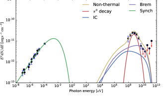
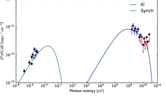
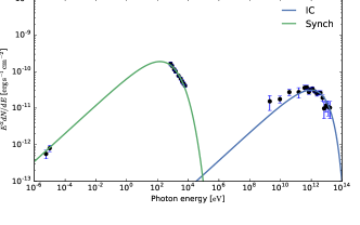
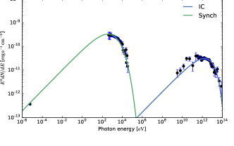
We apply naima, a python-based package, for computing non-thermal radiation processes and fitting the spectral energy distributions Zabalza (2015). It uses Markov-Chain Monte Carlo emcee sampling Foreman-Mackey et al. (2013) to find best-fit parameters of physical radiation models and thus determines the radiation mechanism behind the observed emission. The parameters of the best-fit models are compiled in Table 2 and the best-fit spectra are shown in Fig. 3.
Different from four SNRs mentioned above, we need other approaches to determine parameters for other SNRs without precise high energy -ray observations. Assuming the radio emissions of SNRs are entirely induced by synchrotron emissions of electrons, Di Mauro et al. (2014) provided an estimation method of as
| (12) |
which relies on spectral index , source distance , magnetic field in SNR and the radio flux at 1 GHz . For the synchrotron emission of electron system, the electron spectral index can be derived from the photon spectral index. Thus we have , where is the radio spectral index. We list and in Table 1. Another critical parameter can only be approximately estimated by several methods, such as Zeeman effect, Faraday rotation, and minimum energy or equipartition. The equipartition or minimum energy method calculates magnetic field only depending on the radio synchrotron emission of source Beck and Krause (2005). It is a useful tool if no other data of the source is available. According to the result of Arbutina et al. (2011), we can obtain the magnetic field of SNR as
| (13) |
where is rest energy of electron, and are defined in Ref. Pacholczyk (1970), is the volume filling factor of radio emission, is the angular radius of SNR which can be found in Green catalog. In Eq. (13), is a parameter depending on and ion abundances of SNR. We adopt a typical value and simple ISM abundance H:He=10:1 in our estimation. Note that this minimum energy method is applicable only for mature SNRs with . For G114.3+00.3 and G127.1+00.5, we take a typical value of . Finally, We follow the method proposed by Yamazaki et al. (2006) to give an estimation to . When the age of a SNR meets yr, synchrotron loss restricts the maximum energy of electrons. Thus we have
| (14) |
where is the shock velocity in unit of which depends on evolution of SNR. See details in Ref. Yamazaki et al. (2006) for the definition of and here we take it to be unit.
| Source | Ref. | |||||
| G065.3+05.7 | 10.6 | 10.5 | 2.16 | 7.2 | 0.77 | - |
| G074.0–08.5 | 9.7 | 10 | 1.99 | 0.072 | 0.63 | Katagiri et al. (2011); Reichardt et al. (2015); Uyanıker et al. (2004) |
| G114.3+00.3 | 30 | 0.14 | 1.98 | 9.3 | 0.02 | - |
| G127.1+00.5 | 30 | 0.52 | 1.86 | 4.6 | 0.12 | - |
| G156.2+05.7 | 13 | 0.83 | 2.06 | 8.4 | 0.09 | - |
| G160.9+02.6 | 2.3 | 130 | 2.15 | 0.065 | 5.66 | Araya (2014); Dwarakanath et al. (1982); Leahy and Tian (2007); Reich et al. (2003) |
| G266.2–01.2 | 8.9 | 9.6 | 2.23 | 25.4 | 0.59 | Aharonian et al. (2007); Duncan and Green (2000); Tanaka et al. (2011) |
| G347.3–00.5 | 11.9 | 5.7 | 2.14 | 31 | 0.48 | Abdo et al. (2011); H.E.S.S. Collaboration et al. (2011); Acero et al. (2009); Federici et al. (2015); Tanaka et al. (2008) |
So far we have estimated parameters for all the sources in Table 1 except for Vela(XYZ), Monogem Ring and Loop I. The results are listed in Table 2. Vela(XYZ) is generally believed to be an important local source of CRs. We discuss it in detail in the next section. For Monogem ring and Loop I, they are classified as possible or probable SNRs by Green Green (2014) and are not included in the catalog due to the lack of understanding to them. We treat them as potential sources of electrons in the next section and set their parameters to be free. Note that all those estimations of SNR parameters rely on the electromagnetic radiations of SNR. These emissions are not produced by electrons observed today but some ’younger’ ones in SNRs. This implies that even if observations of photon emission are precise enough, the derived electron parameters may be different from those of injected electrons due to the variation of parameters along with the evolution of SNRs. Therefore the aim of our estimation is to give some reference values for electron injection parameters, but far from to ’determine’ them.
II.3 PWN as Electron and Positron Source
Pulsars are known to be the most important astrophysical sources of high energy electron/positron pairs in the Galaxy Della Torre et al. (2013). They produce relativistic wind carrying charged particles at the cost of their spin-down energy Rees and Gunn (1974). Since pulsar is formed in SN explosion, it is initially surrounded by its companion SNR. When the relativistic pulsar wind impacts on the cold SN ejecta which expands with a slower velocity, a termination shock is formed besides a forward shock. The termination shock propagates inward and reaches the radius where the outward pressure of pulsar wind balances the internal pressure of the shocked bubble (see Ref. Gaensler and Slane (2006) and references therein). The shocked region is dubbed the pulsar wind nebula (PWN). After particles inter the PWN, they are confined by the magnetic field here for a long period, until the crushing of the PWN. Thus the spectrum of electrons and positrons injected into ISM should be the spectrum inside the PWN when it is disrupted, other than the spectrum inside the magnetosphere of pulsar Malyshev et al. (2009). Like SNRs, pulsars can be divided into local pulsars and smooth distant components. Delahaye et al. (2010) find that the contribution from pulsar background is negligible compared to those from local ones, thus we do not take the former into account in our calculation. Parameters of nearby pulsars can be found in the ATNF catalog Taylor et al. (1993).
We assume the injection spectra of PWNs have the same form of Eq. (11); a burst-like injection spectrum is also adopted. Note that the spectral index used here is associated with the PWN, and cannot be derived from the spectral index of the pulsed radio emission from pulsar given in the ATNF catalog. Thus if the radio spectral index of PWN is not available, we set as a free parameter in the following fittings. The normalization parameter is linked to the spin-down energy dissipated by pulsar by:
| (15) |
where GeV and is the efficiency of energy conversion treated as another free parameter. The spin-down luminosity evolves with the age of pulsar as Pacini and Salvati (1973), where is the initial spin-down luminosity, is the spin-down time scale of the pulsar, assumed to be 10 kyr in our work. Integrating with time, we get the expression of spin-down energy , where and can be found in ATNF catalog. For the cut-off energy, We take TeV following the work of Ref. Di Mauro et al. (2014).
II.4 Secondary Electrons and Positrons
Secondary electrons and positrons are created by inelastic collision between CR nuclei and ISM. The CR nuclei mainly consist of protons and particles while H and He are major components of ISM. As can be seen from the AMS-02 result, the positron fraction is smaller than 10% below GeV, where secondary positrons should contribute less than 10%. Since the spallation process produces more positrons than electrons, secondary electrons possess a further smaller percentage comparing to the total electron intensity in the range mentioned above. Thus we neglect the secondary electron component and concentrate on secondary positrons. In this part, our calculation follows the method of Ref. Delahaye et al. (2009). The source function of secondary is assumed to be steady and homogeneous in a slab geometry:
| (16) |
so that the propagation equation can be solved semi-analytically with a relatively simple form (see Delahaye et al. (2009) for details). In Eq. (16), and mark the species of CR nuclei and ISM gas respectively. The number density of ISM is set to be and . The intensities of incident CR nuclei are donated by which can be estimated by the observed intensities at earth. We employ the expression of proposed by Shikaze et al. (2007). Di Mauro et al. (2014) fit the AMS-02 data of proton and Helium to refresh the parameters in the model of . For differential scattering cross-section , Kamae et al. (2006) provides functional formulae for proton-proton collision. Empirical rescaling based on this result are applied to estimate cross-section of collision between other species Norbury and Townsend (2007). Besides, we introduce a free parameter to rescale the secondary intensity, considering the uncertainty in the calculation above, to accommodate the data.
III Fitting to the AMS-02 data
Up to now, AMS-02 provides the most precise measurement of leptonic spectra below 1 TeV. We attempt to perform global fittings to all the leptonic data released by the AMS-02 Collaboration, including the positron fraction, positron plus electron spectrum, positron spectrum and electron spectrum Accardo et al. (2014); Aguilar et al. (2014a, b). The global fitting is useful to set stringent constraints for astrophysical contributors, and leads to a self-consistent picture Yuan et al. (2015).
Astrophysical components considered in our model have been discussed in the previous section, including background SNRs as main contributors of electrons in low energy range, local SNRs as dominant contributors of electrons in higher energy range, secondary positrons which dominate low energy part of positron spectrum, and local PWNs as predominant components in higher energy range of positrons.
In this section, we explain the AMS-02 data by using several astrophysical source models. The characteristic of each model depends on which sources are chosen to be predominant local SNRs. We can see below that according to the calculation in the previous section, local SNRs listed in Table 2 hardly have significant contributions to electron intensity within the energy range of AMS-02. They would not play the role of predominant local sources in this section; we simply add their contributions for each model.
Positrons contribute only of the total intensity. We would like to simplify the constitution of positron spectrum, and use a single PWN to fit the high energy part of spectrum. Di Mauro et al. (2014) have already given a ’single-source’ analysis in their work and find that Geminga is the most proper one among their candidates. However, due to the old age of Geminga (342 kyr), a spectral roll-off may appear below 1 TeV. Thus if Geminga is chosen as the single PWN, it may induce a slight break in spectrum below 1 TeV.
Another famous pulsar B0656+14, also namely Monogem, is believed to be associated with Monogem Ring. It lies at a distance of 0.28 kpc with an age of 112 kyr which is younger than Geminga Taylor et al. (1993). Monogem has the potential to significantly contribute to the positron spectrum from 100 GeV to 1 TeV (see Table 4 of Ref. Delahaye et al. (2010)). Also, we can see from Figure 2 of Ref. Di Mauro et al. (2014), the spectrum of Monogem has a similar shape with that of total PWNs in the ATNF catalog. Therefore we expect a PWN with the similar distance and age as Monogem can play a role as the single positron source.
We would show in following subsections that Monogem does well in the fittings as a single positron source. Comparing with the total spin-down energy of Geminga erg and the required of only 0.27 in the ’single source’ model in Ref. Di Mauro et al. (2014), the fittings for Monogem requires a large (0.60.8 in our models) due to its low spin-down energy of erg. However, Monogem can extent its electron/positron spectra to higher energies than Geminga because of its smaller lifetime, and is helpful to explain the cut-off indicated by HESS and VERITAS data. In this work, we take Monogem as the single positron source in our fittings.
Hence, for different models shown below, the common free parameters are and for SNR background, rescaling parameter for secondary positron, and for Monogem and a solar modulation potential to accommodate data below tens of GeV.


III.1 Vela YZ
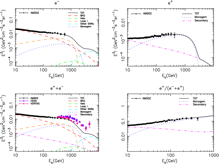
It is widely believed that the famous and well studied SNR Vela is an important local source of Galactic CRs due to its appropriate age and distance and its strong radio emission Kobayashi et al. (2004); Di Mauro et al. (2014). Fig. 4 shows the contours of electron intensity as a function of and of source at different energy, assuming typical input energy (erg), spectral index (2.0) and cut-off energy (10 TeV) of electrons. Every source in Table 1 is marked in Fig. 4. It is clearly that Vela predominates over other local SNRs above hundreds of GeV, and this is where the observed electron excess to continuous SNR model appears.
Vela shows a shell-like radio structure consisting of three principle regions, dubbed Vela X, Y and Z Rishbeth (1958). A weaker component Vela W observed by Alvarez et al. (2001) is not considered in our work. Milne (1968) find the spectrum of Vela X was remarkably flat than that of Vela Y and Z. This unusual spectrum was first explained by Weiler and Panagia (1980). They argued that Vela X should belong to plerions and PWNs like Crab, rather than shell-type SNRs like its siblings Vela Y and Z. This point of view has been accepted in later works. Consequently, when we estimate the contribution from Vela SNR, we ought to divide Vela X from Vela YZ. PWNs have different mechanisms of acceleration and evolution from shell-type SNRs. This means that they cannot share parameters, such as spectral index or cut-off energy, with the later.
In the first model, we set Vela YZ as the unique predominant SNR and aim to check if it can give a good interpretation to AMS-02 data. As suggested by Ref. Di Mauro et al. (2014), we fix the magnetic field to be 30 G and cut-off energy to be 2 TeV. In the Green catalog of SNRs, the radio spectral index of Vela is denoted as ’varies’ perhaps due to the discrepancy between Vela X and YZ. We put spectral index of Vela YZ into the group of free parameters in this model. A free leads to the uncertainty of . The radio flux of Vela YZ at 960 MHz is measured to be 1100 Jy Alvarez et al. (2001), so we set Jy here as an estimation. We seek the best-fit model by minimizing chi-squared statics between model and data points. The result of global fitting to AMS-02 data are shown in Fig. 5. In each sub-graph, all the components are drawn to show their contribution and black solid line represents the fitting result. The best-fit reduced is 0.473 for 182 degrees of freedom (d.o.f.), while the best-fit parameters are compiled in Table 3. Solar modulation converges to zero in this case.
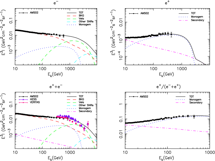
As can be seen that this model well explains the AMS-02 data. The best-fit radio spectral index of Vela YZ seems reasonable, as it is close to the typical value 0.5. Di Mauro et al. (2014) also fit the four leptonic observables of AMS-02 simultaneously and obtain fairly good result. However, our model has two main differences from theirs. First, the propagation parameters they adopted is the MED model proposed by Ref. Donato et al. (2004) which is based on the B/C analysis performed in Ref. Maurin et al. (2001), and the nuclei data behind is taken from earlier balloon and space experiments; as described in Sec. II.1, we include the latest B/C data from AMS-02 in our calculation of propagation parameters. Besides, Vela X and YZ are assumed to provide a whole SNR contribution in their fittings. As mentioned above, these objects may not share the same spectral index, cut-off energy, and normalization parameter . If the contribution of Vela X is considered in the energy range covered by AMS-02, it should have contributed to positron intensity due to its PWN nature, and would not induce a spectral structure at high energies above TeV.
| Model | ||||||||
|---|---|---|---|---|---|---|---|---|
| Vela | 0 | 0.473 |
| Model | [erg] | [TeV] | ||||||||
|---|---|---|---|---|---|---|---|---|---|---|
| 0.398 | ||||||||||
| 0.396 |
| Model | [erg] | [TeV] | ||||||||
|---|---|---|---|---|---|---|---|---|---|---|
| 0.401 | ||||||||||
| 0.400 |
III.2 Vela YZ + Monogem Ring
In this model, we attempt to investigate the parameters of Vela YZ at first, rather than taking typical values as in the previous model. The geometry of Vela SNR can be sketched by two hemisphere with different scales due to the asymmetrical density distribution of its surrounding medium Sushch and Hnatyk (2014). Vela Y and Z are located in the north-east(NE) part. Assuming the equilibrium between thermal pressure and magnetic pressure, Sushch and Hnatyk (2014) give an estimation of with the formula , where density and temperature are derived by Ref. Sushch et al. (2011). We still cite Eq. (14) to calculate cut-off energy. But instead of taking typical value , we choose estimated by Ref. Sushch et al. (2011). The principle behind this estimation is the expression of shock radius as a function of the age of SNR given by Ref. White and Long (1991). We get TeV. For of Vela YZ, Dwarakanath (1991) claims a value of 0.53 combining his 34.5 MHz observation and other observations up to 2700 MHz. The latest work about radio spectrum of Vela is done in Ref. Alvarez et al. (2001). The authors of Ref. Alvarez et al. (2001) included more data points at other frequencies while subtracted the flux density at 34.5 MHz for the probable absorption of this measurement. The of Vela YZ is derived to be 0.735 in this work. For , is derived to be 800 Jy; while for , we derive Jy.

Fig. 6 shows the comparison between the electron spectra of Vela YZ with parameters in the previous model (solid line) and parameters in this model (dashed line for and dot-dashed line for ). If we take our parameters estimated above and still use Vela YZ as the only predominant SNR in the fitting, excesses of and data would arise in hundreds of GeV, especially for the case . Thus, we need to find a proper SNR as a cooperator in this case. Fig. 5 indicates SNRs listed in Table 2 hardly have influence on electron intensity in the energy range of AMS-02, as we mentioned above. From Fig. 4, we can see Monogem ring and Loop I are the potential electron contributors up to 1 TeV. We would like to examine Monogem ring in this model.
Monogem Ring (MR) is a large shell-like structure in soft X-ray band with a diameter Plucinsky et al. (1996). Green does not include large X-ray regions with scales larger than in his catalog Green (2014), thus MR does not appear there. Assuming MR is in its adiabatic phase, Plucinsky et al. (1996) derives parameters of MR with observable quantities and its distance, applying Sedov-Taylor model of SNR. Plucinsky (2009) points out 300 pc should be a reasonable approximation for distance of MR, and consequently an age of yr and an initial explosion energy erg. Apart from this, we possess poor knowledge of MR to constrain its radio spectral index, total energy converted into electrons, or cut-off energy. We add these three quantities, , and to free parameters in this scenario.
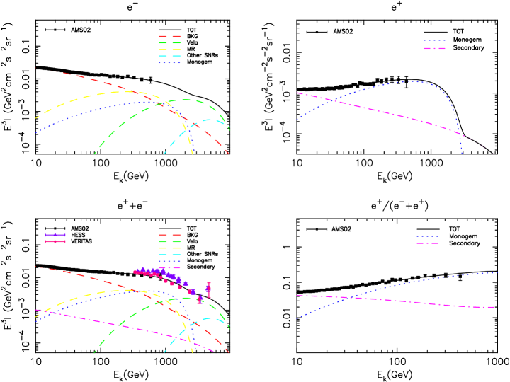
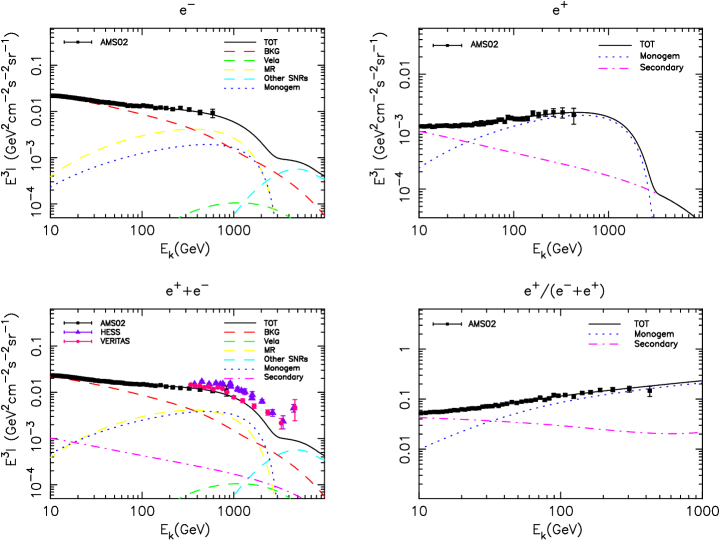
Two global fittings are done with and , and fitting results are plotted in Fig. 7 and Fig. 8 respectively. For the case , the best-fit reduced is 0.398 for 180 d.o.f; if we take the latest value , the result becomes for 180 d.o.f. Best-fit parameters are shown in Table 3 for both cases. It can be seen, good fitting results to AMS-02 data are achieved when MR joins in the model. In and spectra, the deviation between these two results with different becomes clear in TeV range.
III.3 Vela YZ + Loop I (NPS)
In this model, we largely repeat the work of the previous model, but replace MR by Loop I. It is well known that there are several Galactic giant radio loops potentially associating with SN events Berkhuijsen et al. (1971); Berkhuijsen (1973); Duncan et al. (1997). Loop I, which was discovered by Large et al. (1962) and named by Berkhuijsen (1971), is the most prominent one among these loops. Although Loop I, with a radius of , is also not included in the Green’s catalog, it has gone through more careful study than MR. The center of Loop I is close to Scorpio-Centaurus OB association where SN events happen. North Polar Spur (NPS) is the most prominent part of Loop I, both in radio and X-ray maps Egger and Aschenbach (1995). However, the visible X-ray contradicts with the age of yr derived by the low expanding velocity of H I surrounding Loop I Bunner et al. (1972); Sofue et al. (1974). Then a reconciliation is raised: Loop I is indeed an old structure, but it has been reheated by younger SN events Borken and Iwan (1977); Egger and Aschenbach (1995). The shock wave from the most recent SN event in Sco-Cen association happened in years ago and gave rise to the X-ray feature of NPS Egger and Aschenbach (1995). The comparison between the continuous shell-like radio structure and the interrupted X-ray structure of Loop I also favors this interpretation. Thus yr should be take as the age of Loop I (NPS) in our work, and adopting the corresponding distance to NPS—100 pc Bingham (1967)—as the distance of this source is more reasonable than taking that of Sco-Cen association (170 pc) as in some earlier researches. Similar to the previous model, free parameters associating with Loop I (NPS) in the following fittings are , and .
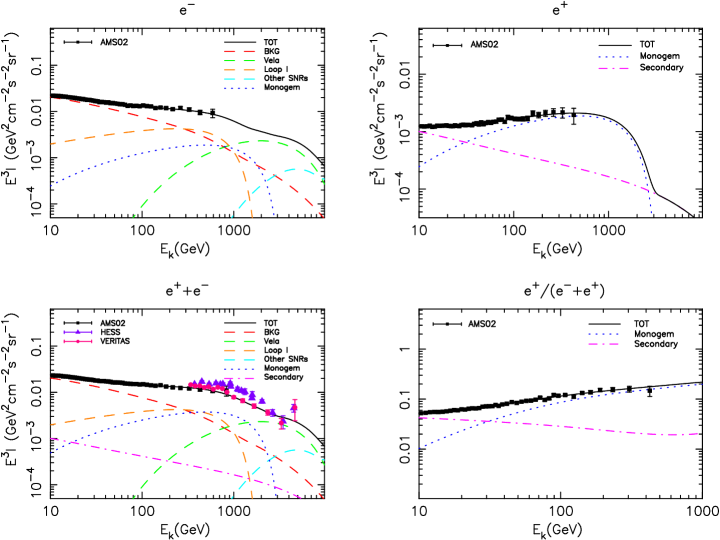
The fitting results are shown in Fig. 9 and Fig. 10 for the case of and , respectively. The best-fit reduced for the former case is 0.401 for 180 d.o.f, while for the later case, for 180 d.o.f. See Table 3 for corresponding best-fit parameters. Comparing with the reduced of the previous model, the fitting effect of this Vela YZ + Loop I scenario has little difference with that of Vela YZ + Monogem Ring scenario.
III.4 Discussion
In this section, we have proposed several source models to fit the leptonic spectra measured by AMS-02. It can be seen that the radio spectral index of Vela YZ is crucial to the situation. Radio measurements from Wilkinson Microwave Anisotropy Probe (WMAP) and Planck may give further constraints on , but processed data for Vela is not available at present. If the radio spectral index of Vela YZ is 0.5, other local SNRs, may not be necessary to join in fitting to the AMS-02 data, as in the Vela YZ model. However, if we choose a value of 0.735, Vela loses its predominance of the local contribution. Since the electron intensity contributed by the PWN is confined by spectrum, other local SNRs, such as MR and Loop I, are needed to reproduce the observed spectrum.
In the Vela YZ + Monogem Ring model, the best fitting lepton energy is erg, near the typical value of erg. However, the low explosion energy of MR derived by Plucinsky (2009) favors a small input energy of electrons, or a very large conversion efficiency of is required. For the Vela YZ + Loop I model, we get a larger input energy for electrons of erg. However, this large value seems not excluded by the initial SN energy of Loop I of erg, which may be produced by several SN events Egger and Aschenbach (1995). Our fitting result of is 0.417, which is smaller than the value of 0.5 given by the radio observation to NPS between 22 and 408 MHz Roger et al. (1999) or between 45 and 408 MHz Guzmán et al. (2011). The measurements between 408 and 1420 MHz get a even larger value of 1.1 Reich and Reich (1988). It is also possible that both MR and Loop I play important roles in the spectrum. This setting may relax the ranges of and somewhat.
IV Electron spectrum above TeV
Now we turn attention to higher energy part beyond the scope of AMS-02. DAMPE is expected to detect electrons/positrons in the range of 5 GeV to 10 TeV Chang (2014). Models proposed in the previous section have already given spectra extending to TeV range, which may be measured in future DAMPE data. However, although these models give different predictions in TeV range depending on the characteristic of Vela YZ, a common decreasing is shown in spectrum up to 10 TeV in each model. This means that these models predict no protruding structure in the highest energy range of DAMPE.
Ground-based Cherenkov telescopes, such as HESS Aharonian et al. (2008, 2009), MAGIC Borla Tridon (2011) and VERITAS Staszak and for the VERITAS Collaboration (2015), have extended the measurement of spectrum to several TeV. These measurements show that a spectral steepening appears above 1 TeV. Furthermore, HESS and the preliminary result of VERITAS have measured a coincident ascending of intensity in TeV, which may imply a feature from local sources. Unfortunately, this tendency comes from only the most energetic data point in both case and no measurement has been taken above 5 TeV. Thus it is the show time for DAMPE to examine this tendency.
In this section, we give additional predictions to electron spectrum above TeV. We would study whether local sources can produce distinctive features in the high energy range covered by DAMPE. Although we do not intend to fit the data of HESS, MAGIC, or VERITAS quantitively, we need to keep in mind that the spectral steepening just beyond 1 TeV could be reproduced in our models.
IV.1 Vela X
There is still an important source which have not been included in our models so far: Vela X, as the sibling of Vela YZ. Vela X is one of the most well studied PWN powered by PSR B0833–45 Weiler and Panagia (1980). It has been covered by observations from radio bands to very high energy -ray bands Alvarez et al. (2001); Markwardt and Ögelman (1997); Mangano et al. (2005); Abramowski et al. (2012); Abdo et al. (2010); Grondin et al. (2013). In morphology, Vela X consists of an extended halo and a small collimated fearture embeded in the halo, e.g., the ’cocoon’. TeV -ray emssion has been detected in the cocoon region by HESS, while Fermi-LAT observations has reported the presence of sub-GeV-peak -ray emssion extending in the halo. de Jager et al. (2008) proposes a model with two populations of electrons to interpret this phenomenon: a high energy component concentrating on the cocoon responsible for X-ray and TeV -ray emssion, and a lower energy component extending in the halo responsible for radio and GeV -ray emssion. Following this idea, assuming the leptonic origin of -ray emssion, Abdo et al. (2010) give a multi-wavelength fitting to the SED of Vela-X. In their results, the cut-off energy of the halo is only 100 GeV which is too low to help Vela-X appearing in TeV range; for the cocoon, although its cut-off energy is high enough, a total lepton energy of erg is too weak to produce significant structure in TeV spectrum.
However, as mentioned above, these electron features derived by photon emission may not describe those electrons we have observed. Hinton et al. (2011) provide an alternative model in which a serious particle escape has happened in the halo while particles in the cocoon are well confined. After staying in confinement status for a long time, PWN begins to interact with the coming reverse shock of SNR. It is the time that PWN crushes and burst-like injection happens. From then on, the halo has been suffering from energy-dependent escape, thus the cut-off energy derived by Fermi-LAT observations is such a small value. From some moment after the PWN crushes, the pulsar starts to inject particles to a new PWN, that is, the cocoon. This explains the dimness of the cocoon for its short time of particle injection.
Hinton et al. (2011) gives an estimation of electron injection spectrum: with an total energy erg. Thus Vela X seems to produce a TeV feature. However, the diffusion coefficient adopted by them ( for energy much larger than 1 GeV) is almost an order of magnitude smaller than ours. If we take our , the intensity from Vela X is much larger, especially at lower energy. The spectral steepening indicated by HESS and VERITAS cannot be reproduced, and even the energy range of AMS-02 would be affected. Since the diffusion scale is proportional to , a larger means a faster propagation and more electrons with lower energy are able to arrive at the Earth. If we want to keep the steepening feature in 1 TeV, an unreasonable young age of Vela X is needed.
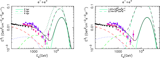
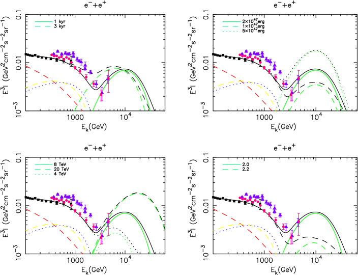
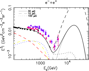
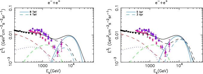
We combine Vela X and each model in the previous section to give new predictions. As discussed above, we have to keep the given by Ref. Hinton et al. (2011) only for Vela X. Fig. 11 shows the predicted spectra. Since there is little difference between the spectral shape of Vela YZ + MR model and Vela YZ + Loop I model, we only draw the former case as representative. The effects of varying injection time of Vela X and diffusion coefficient are also shown in Fig. 11. We take three different injection age of Vela X as 2 kyr, 3 kyr, and 4 kyr. Note these ages are still observed ages, keeping consistent with those listed in Table 1. With injection age increasing, the steepening structure in 1 TeV is gradually filled up. This requires an injection age less than 5 kyr, according with the theory that reverse shock has recently crushed the PWN Blondin et al. (2001). Moreover, Fig. 11 indicates the spectrum of Vela X depends sensitively on diffusion coefficient (we double the for comparison). With the data of DAMPE and a clearer picture of the particle escape of PWN in the future, Vela X may become a potential tool to constrain diffusion coefficient in high energy.
IV.2 Vela YZ
Naturally, following Vela X, the next question is if Vela YZ can play an important role in the highest energy part of DAMPE. The work of Ref. Kobayashi et al. (2004) shows the possibility of this scenario after considering the release time of electrons in SNR, although they do not make a distinction between Vela X and Vela YZ. Erlykin and Wolfendale (2002) believe that electrons start their propagation after the expansion phase of SNR which hold a typical time scale of 200 yr. This time delay is too small to change the electron spectrum of Vela YZ. Alternatively, Dorfi (2000) point out particles begin to escape from the shock front when the SNR dissolves in the ISM, i.e., when the velocity of the shock has dropped to the mean Alfvn velocity of ISM. However, even we take a very low number density of , the derived release time is several times of yr which is larger than the observed age of Vela YZ or the typical time scale of Sedov phase. To insure electrons have already escaped from Vela YZ, we should control its release time not longer than yr, corresponding to a least observed age 1 kyr. The total input energy of Vela YZ is much smaller than that of Vela X, it should be at the magnitude of erg. When the electron acceleration is synchrotron loss limited, the cut-off energy decreases with the age growth of SNR. Since TeV is derived by observations of electromagnetic radiation, the injection spectrum of electrons should have a larger cut-off energy. Similarly, higher energy electrons should suffer heavier energy loss, which causes softening of spectrum with the growth of trapped time of electrons. Thus the spectral index of injection spectrum may smaller than that derived by radio observations.
We set kyr, erg, TeV and as fiducial values and use some other values of these parameters to show spectral variation in Fig. 12. In this figure, we apply Vela YZ + Monogem Ring model () in Sec. III. In this model Vela YZ can bring ascending or relatively flat spectral features just below 10 TeV, as shown in Fig. 12. We can imply from this figure that if the radio spectral index is taken 0.735 here, Vela YZ will have no chance to produce spectral feature in TeV.
IV.3 Vela Jr.
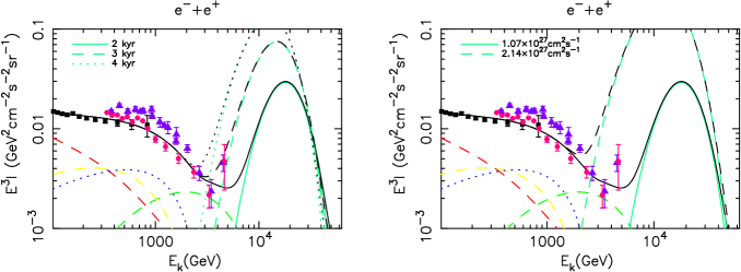
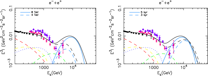
Besides Vela XYZ, other candidates producing prominent structure in the TeV range should be selected from Table 2. Fig. 13 shows intensity of each SNR listed in Table II, along with the data of HESS and VERITAS. Cygnus Loop and HB9 do not appear in the scope of Fig. 13 because of their very low cut-off energy. To affect the spectrum in TeV, Vela Jr. seems to need least parametric adjustment, namely, a larger input energy to leptons. Thus we examine Vela Jr. as an example.
Vela Jr. locates in the southeastern corner of Vela on the sky map, but at a farther distance of 750 pc. Vela Jr. is one of those sources whose parameters are estimated by fitting the multi-wavelength emission in Sec. II.2.2. Tanaka et al. (2011) and Lee et al. (2013) also conducted broadband analysis to Vela Jr. in recent years. As there have been discussions about magnetic field of Vela Jr., and can be estimated by Eq. (12) and Eq. (14). We put aside our fitting result to parameters of Vela Jr. temporarily. Chandra has detected spindly filamentary structure in Vela Jr. Bamba et al. (2005). This thin structure is interpreted by efficient synchrotron cooling of CR electrons in a strong local magnetic field of G Berezhko et al. (2009). However, if broadband emission is modeled by leptonic scenario, a magnetic field of G is required to explain the synchrotron to inverse Compton flux ratio. Thus we take three different magnetic fields of G, G and a typical value G adopted in Ref. Di Mauro et al. (2014). Here and are taken to be 0.3 and 50 Jy, as given in Table 1, to calculate . We take the upper limit of the age of Vela Jr., i.e. an observed age of 4.3 kyr.
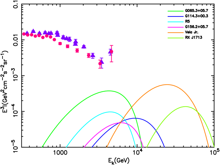
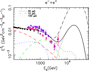
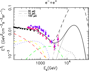
The predicted spectrum of Vela Jr. combining with Vela YZ and Vela YZ + Monogem Ring models (of course original Vela Jr. subtracted) are shown in Fig. 14. The input leptonic energy corresponding to magnetic field of G, G and G are erg, erg and erg, respectively. For the case of G, Vela Jr. cannot produce prominent feature in TeV; when G, the spectral feature given by Vela Jr. is remarkable enough, but it needs a total leptonic energy much higher than the typical value of erg. The result given by G may be what we’d like to see. However, we should note the of Vela Jr. is derived by the radio flux of only two wave bands, which is quite unreliable, and the value of will give a significant influence to the total leptonic energy of Vela Jr. with the method used here. In fact, the parameters given by the leptonic model of Ref. Tanaka et al. (2011) is similar to the result of our broadband fitting (the differences may be due to the consideration of the energy loss between injection electrons and radiation electrons in the work of Tanaka et al. (2011)). Lee et al. (2013) also found the leptonic model is clearly superior to hadronic model. Thus broadband fitting may give better constraint to parameters of Vela Jr., which disfavor Vela Jr. as a prominent contributor in TeV.
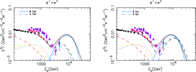
IV.4 Cygnus Loop
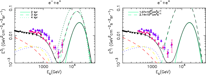
Cygnus Loop is one of the closest SNRs to the Earth (540 pc) and is considered as an important local CR accelerator second only to Vela Di Mauro et al. (2014). However, its steep GeV spectrum observed by Fermi-LAT (see Fig. 3) indicates a very low cut-off energy of electron spectrum, thus it cannot play a part in the models above. Cut-off energy derived by Eq. (14) is at least several TeV for Cygnus Loop, so it is possible that Cygnus Loop has undergone serious particle escape similar to the case of Vela X. Unfortunately, although Cygnus Loop has been carefully studied in X-ray band with the help of XMM-Newton and Suzaku Uchida et al. (2008); Leahy and Hassan (2013), its global X-ray spectrum is not available. Thus we cannot give further inference from the broadband spectrum of Cygnus Loop as Vela X. Here we assume cut-off energy of TeV for Cygnus Loop, which is the precondition for Cygnus Loop to contribute significantly in TeV range. Besides, to preserve the spectral steepening in 1 TeV, considerable release time is needed for Cygnus Loop. We keep others parameters given by broadband fitting unchanged. Like the former cases, we combine Cygnus Loop with models given in Sec. III and also show the effects of varying cut-off energy and observed age of Cygnus Loop in Fig. 15. In the left panels, observed age is fixed at 5 kyr, while in the right panels, cut-off energy of Cygnus Loop is set to be 8 TeV.
IV.5 Discussion
As discussed in the last section, it is hard to tell which local SNR dominates the electron excess in the energy range of AMS-02, since the spectra of local SNRs are mixed with that of the SNR background below 1 TeV. However, things are different above the TeV scale that can be covered by DAMPE. The contributions from the background SNRs may be very small in this energy range. If we get a distinctive spectrum above several TeV, we may determine the origin of these cosmic ray electrons. Of course, it is also possible that more than one sources shape the high energy electron spectrum, then the situation becomes complicated.
In order to produce clear features at the spectrum beyond TeV, a small particle propagation time and a high energy cut-off of injection electrons are essential. We have considered the Vela X, Vela YZ, Vela Jr. and Cygnus Loop as possible candidates contributing to cosmic electrons above TeV in this section. Except for very young sources like Vela Jr., other three candidates need an additional release time. We find that Vela X and Vela Jr. may provide a very sharp rise in the spectrum at a few TeV due to the very young components, while the Vela YZ and Cygnus Loop may show much smoother feature at the similar energy. Thus with the basis of a kyr injection age and a TeV cut-off energy, the total leptonic injection energy of a source is the key factor to produce a sharp spectral structure in the high energy range covered by DAMPE.
V Summary
In this paper, we have given predictions to CR electron (plus positron) spectrum above TeV basing on the elaborate analysis of the local astrophysical sources, especially the local SNRs. In order to obtain a complete picture, we ensure the consistency between the predicted spectra and present experimental results below TeV by performing global fittings to all the latest leptonic AMS-02 data. We find that Vela YZ could act as the dominator just below TeV because of its proper age and distance. However, it should be emphasized that the determination of the injection spectral index of Vela YZ, which still has some uncertainties, is crucial to fittings. We discuss different scenarios to fit AMS-02 data corresponding to different values of the spectral index of Vela YZ. Other SNRs, such as Monogem Ring and Loop I, are also introduced, if Vela YZ dose not provide the dominant contribution to the AMS-02 electron results.
Basing on the fitting results, we discuss the parameters of several local sources, and give further expectations of the electron spectrum above TeV. Adopting different possible values for those parameters, we predict either sharp or relatively flat electron spectral features, comparing with the monotonic decreasing spectra of the models in Sec. III. All these models are ready for the examination at high energy CR electron detectors, such as DAMPE, which can reach the energy as high as TeV. The spectrum measurement of DAMPE and future anisotropy measurements Manconi et al. (2016) may reveal the origin of the high energy CR electrons. These results will also be important for probing the mechanism of CR acceleration in the sources.
Acknowledgements.
This work is supported by the National Natural Science Foundation of China under Grants No. 11475189, 11475191, and by the 973 Program of China under Grant No. 2013CB837000, and by the National Key Program for Research and Development (No. 2016YFA0400200).References
- Aguilar et al. (2013) M. Aguilar, G. Alberti, B. Alpat, A. Alvino, G. Ambrosi, K. Andeen, H. Anderhub, L. Arruda, P. Azzarello, A. Bachlechner, et al., Physical Review Letters 110, 141102 (2013).
- Adriani and the others (2009) O. Adriani et al., Nature 458, 607 (2009), arXiv:0810.4995 .
- Adriani and the others (2011) O. Adriani et al., Physical Review Letters 106, 201101 (2011), arXiv:1103.2880 [astro-ph.HE] .
- Abdo and the others (2009) A. A. Abdo et al., Physical Review Letters 102, 181101 (2009), arXiv:0905.0025 [astro-ph.HE] .
- Ackermann and the others (2010) M. Ackermann et al., Phys. Rev. D 82, 092004 (2010), arXiv:1008.3999 [astro-ph.HE] .
- Chang et al. (2008) J. Chang, J. H. Adams, H. S. Ahn, G. L. Bashindzhagyan, M. Christl, O. Ganel, T. G. Guzik, J. Isbert, K. C. Kim, E. N. Kuznetsov, M. I. Panasyuk, A. D. Panov, W. K. H. Schmidt, E. S. Seo, N. V. Sokolskaya, J. W. Watts, J. P. Wefel, J. Wu, and V. I. Zatsepin, Nature 456, 362 (2008).
- Feng et al. (2014) L. Feng, R.-Z. Yang, H.-N. He, T.-K. Dong, Y.-Z. Fan, and J. Chang, Physics Letters B 728, 250 (2014), arXiv:1303.0530 [astro-ph.HE] .
- Li et al. (2015) X. Li, Z.-Q. Shen, B.-Q. Lu, T.-K. Dong, Y.-Z. Fan, L. Feng, S.-M. Liu, and J. Chang, Physics Letters B 749, 267 (2015), arXiv:1412.1550 [astro-ph.HE] .
- Lin et al. (2015) S.-J. Lin, Q. Yuan, and X.-J. Bi, Phys. Rev. D 91, 063508 (2015), arXiv:1409.6248 [astro-ph.HE] .
- Shen (1970) C. S. Shen, Astrophys. J. Lett. 162, L181 (1970).
- Atoyan et al. (1995) A. M. Atoyan, F. A. Aharonian, and H. J. Völk, Phys. Rev. D 52, 3265 (1995).
- Kobayashi et al. (2004) T. Kobayashi, Y. Komori, K. Yoshida, and J. Nishimura, Astrophys. J. 601, 340 (2004), astro-ph/0308470 .
- Di Mauro et al. (2014) M. Di Mauro, F. Donato, N. Fornengo, R. Lineros, and A. Vittino, J. Cosmol. Astropart. Phys. 4, 006 (2014), arXiv:1402.0321 [astro-ph.HE] .
- Jóhannesson et al. (2016) G. Jóhannesson, R. Ruiz de Austri, A. C. Vincent, I. V. Moskalenko, E. Orlando, T. A. Porter, A. W. Strong, R. Trotta, F. Feroz, P. Graff, and M. P. Hobson, Astrophys. J. 824, 16 (2016), arXiv:1602.02243 [astro-ph.HE] .
- Aharonian et al. (2008) F. Aharonian et al., Physical Review Letters 101, 261104 (2008), arXiv:0811.3894 .
- Aharonian et al. (2009) F. Aharonian et al., Astron. Astrophys. 508, 561 (2009), arXiv:0905.0105 [astro-ph.HE] .
- Staszak and for the VERITAS Collaboration (2015) D. Staszak and for the VERITAS Collaboration, ArXiv e-prints (2015), arXiv:1508.06597 [astro-ph.HE] .
- Chang (2014) J. Chang, Chin. J. Space Sci. 34, 550 (2014).
- Delahaye et al. (2010) T. Delahaye, J. Lavalle, R. Lineros, F. Donato, and N. Fornengo, Astron. Astrophys. 524, A51 (2010), arXiv:1002.1910 [astro-ph.HE] .
- Davis et al. (2000) A. J. Davis, R. A. Mewaldt, W. R. Binns, E. R. Christian, A. C. Cummings, J. S. George, P. L. Hink, R. A. Leske, T. T. von Rosenvinge, M. E. Wiedenbeck, and N. E. Yanasak, in Acceleration and Transport of Energetic Particles Observed in the Heliosphere, American Institute of Physics Conference Series, Vol. 528, edited by R. A. Mewaldt, J. R. Jokipii, M. A. Lee, E. Möbius, and T. H. Zurbuchen (2000) pp. 421–424.
- AMS-02 collaboration (2013) AMS-02 collaboration, in International Cosmic Ray Conference (2013).
- Connell (1998) J. J. Connell, Astrophys. J. Lett. 501, L59 (1998).
- Yanasak et al. (2001) N. E. Yanasak, M. E. Wiedenbeck, R. A. Mewaldt, A. J. Davis, A. C. Cummings, J. S. George, R. A. Leske, E. C. Stone, E. R. Christian, T. T. von Rosenvinge, W. R. Binns, P. L. Hink, and M. H. Israel, Astrophys. J. 563, 768 (2001).
- Lukasiak (1999) A. Lukasiak, International Cosmic Ray Conference 3, 41 (1999).
- Simpson and Garcia-Munoz (1988) J. A. Simpson and M. Garcia-Munoz, Space Sci. Rev. 46, 205 (1988).
- Hams et al. (2004) T. Hams, L. M. Barbier, M. Bremerich, E. R. Christian, G. A. de Nolfo, S. Geier, H. Göbel, S. K. Gupta, M. Hof, W. Menn, R. A. Mewaldt, J. W. Mitchell, S. M. Schindler, M. Simon, and R. E. Streitmatter, Astrophys. J. 611, 892 (2004).
- Schlickeiser and Ruppel (2010) R. Schlickeiser and J. Ruppel, New Journal of Physics 12, 033044 (2010), arXiv:0908.2183 [astro-ph.HE] .
- Ginzburg and Ptuskin (1976) V. L. Ginzburg and V. S. Ptuskin, Reviews of Modern Physics 48, 161 (1976).
- Malyshev et al. (2009) D. Malyshev, I. Cholis, and J. Gelfand, Phys. Rev. D 80, 063005 (2009), arXiv:0903.1310 [astro-ph.HE] .
- Lorimer (2004) D. R. Lorimer, in Young Neutron Stars and Their Environments, IAU Symposium, Vol. 218, edited by F. Camilo and B. M. Gaensler (2004) p. 105, astro-ph/0308501 .
- Strong and Moskalenko (1998) A. W. Strong and I. V. Moskalenko, Astrophys. J. 509, 212 (1998), astro-ph/9807150 .
- Green (2014) D. A. Green, Bulletin of the Astronomical Society of India 42, 47 (2014), arXiv:1409.0637 [astro-ph.HE] .
- Gorham et al. (1996) P. W. Gorham, P. S. Ray, S. B. Anderson, S. R. Kulkarni, and T. A. Prince, Astrophys. J. 458, 257 (1996).
- Mavromatakis et al. (2002) F. Mavromatakis, P. Boumis, J. Papamastorakis, and J. Ventura, Astron. Astrophys. 388, 355 (2002), astro-ph/0204079 .
- Xiao et al. (2009) L. Xiao, W. Reich, E. Fürst, and J. L. Han, Astron. Astrophys. 503, 827 (2009), arXiv:0904.3170 .
- Blair et al. (2005) W. P. Blair, R. Sankrit, and J. C. Raymond, Astron. J. 129, 2268 (2005).
- Sun et al. (2006) X. H. Sun, W. Reich, J. L. Han, P. Reich, and R. Wielebinski, Astron. Astrophys. 447, 937 (2006), astro-ph/0510509 .
- Han et al. (2013) J. L. Han, W. Reich, X. H. Sun, X. Y. Gao, L. Xiao, W. B. Shi, P. Reich, and R. Wielebinski, International Journal of Modern Physics Conference Series 23, 82 (2013), arXiv:1202.1875 .
- Kothes et al. (2006) R. Kothes, K. Fedotov, T. J. Foster, and B. Uyanıker, Astron. Astrophys. 457, 1081 (2006).
- Yar-Uyaniker et al. (2004) A. Yar-Uyaniker, B. Uyaniker, and R. Kothes, Astrophys. J. 616, 247 (2004), astro-ph/0408386 .
- Joncas et al. (1989) G. Joncas, R. S. Roger, and P. E. Dewdney, Astron. Astrophys. 219, 303 (1989).
- Leahy and Tian (2006) D. Leahy and W. Tian, Astron. Astrophys. 451, 251 (2006), astro-ph/0601487 .
- Katsuda et al. (2009) S. Katsuda, R. Petre, U. Hwang, H. Yamaguchi, K. Mori, and H. Tsunemi, Publications of the Astronomical Society of Japan 61, S155 (2009), arXiv:0902.1782 .
- Reich et al. (1992) W. Reich, E. Fuerst, and E. M. Arnal, Astron. Astrophys. 256, 214 (1992).
- Xu et al. (2007) J. W. Xu, J. L. Han, X. H. Sun, W. Reich, L. Xiao, P. Reich, and R. Wielebinski, Astron. Astrophys. 470, 969 (2007).
- Yamauchi et al. (2000) S. Yamauchi, J. Yokogawa, H. Tomida, K. Koyama, and K. Tamura, in Broad Band X-ray Spectra of Cosmic Sources, edited by K. Makishima, L. Piro, and T. Takahashi (2000) p. 567.
- Leahy and Tian (2007) D. A. Leahy and W. W. Tian, Astron. Astrophys. 461, 1013 (2007), astro-ph/0606598 .
- Reich et al. (2003) W. Reich, X. Zhang, and E. Fürst, Astron. Astrophys. 408, 961 (2003).
- Plucinsky et al. (1996) P. P. Plucinsky, S. L. Snowden, B. Aschenbach, R. Egger, R. J. Edgar, and D. McCammon, Astrophys. J. 463, 224 (1996).
- Plucinsky (2009) P. P. Plucinsky, in American Institute of Physics Conference Series, Vol. 1156, edited by R. K. Smith, S. L. Snowden, and K. D. Kuntz (2009) pp. 231–235.
- Alvarez et al. (2001) H. Alvarez, J. Aparici, J. May, and P. Reich, Astron. Astrophys. 372, 636 (2001).
- Caraveo et al. (2001) P. A. Caraveo, A. De Luca, R. P. Mignani, and G. F. Bignami, Astrophys. J. 561, 930 (2001), astro-ph/0107282 .
- Cha et al. (1999) A. N. Cha, K. R. Sembach, and A. C. Danks, Astrophys. J. Lett. 515, L25 (1999), astro-ph/9902230 .
- Miceli et al. (2008) M. Miceli, F. Bocchino, and F. Reale, Astrophys. J. 676, 1064-1072 (2008), arXiv:0712.3017 .
- Aschenbach (1998) B. Aschenbach, Nature 396, 141 (1998).
- Iyudin et al. (1998) A. F. Iyudin, V. Schönfelder, K. Bennett, H. Bloemen, R. Diehl, W. Hermsen, G. G. Lichti, R. D. van der Meulen, J. Ryan, and C. Winkler, Nature 396, 142 (1998).
- Katsuda et al. (2008) S. Katsuda, H. Tsunemi, and K. Mori, Astrophys. J. Lett. 678, L35 (2008), arXiv:0803.3266 .
- Redman and Meaburn (2005) M. P. Redman and J. Meaburn, Mon. Not. Roy. Astron. Soc. 356, 969 (2005).
- Bingham (1967) R. G. Bingham, Mon. Not. Roy. Astron. Soc. 137, 157 (1967).
- Egger and Aschenbach (1995) R. J. Egger and B. Aschenbach, Astron. Astrophys. 294, L25 (1995), astro-ph/9412086 .
- Lazendic et al. (2004) J. S. Lazendic, P. O. Slane, B. M. Gaensler, S. P. Reynolds, P. P. Plucinsky, and J. P. Hughes, Astrophys. J. 602, 271 (2004), astro-ph/0310696 .
- Morlino et al. (2009) G. Morlino, E. Amato, and P. Blasi, Mon. Not. Roy. Astron. Soc. 392, 240 (2009), arXiv:0810.0094 .
- Yuan et al. (2011) Q. Yuan, S. Liu, Z. Fan, X. Bi, and C. L. Fryer, Astrophys. J. 735, 120 (2011), arXiv:1011.0145 [astro-ph.HE] .
- Porter et al. (2006) T. A. Porter, I. V. Moskalenko, and A. W. Strong, Astrophys. J. Lett. 648, L29 (2006), astro-ph/0607344 .
- Petrosian and Liu (2004) V. Petrosian and S. Liu, Astrophys. J. 610, 550 (2004), astro-ph/0401585 .
- Zabalza (2015) V. Zabalza, ArXiv e-prints (2015), arXiv:1509.03319 [astro-ph.HE] .
- Foreman-Mackey et al. (2013) D. Foreman-Mackey, D. W. Hogg, D. Lang, and J. Goodman, Publications of the Astronomical Society of Pacific 125, 306 (2013), arXiv:1202.3665 [astro-ph.IM] .
- Beck and Krause (2005) R. Beck and M. Krause, Astronomische Nachrichten 326, 414 (2005), astro-ph/0507367 .
- Arbutina et al. (2011) B. Arbutina, D. Urošević, M. Andjelić, and M. Pavlović, Mem. S.A.It. 82, 822 (2011).
- Pacholczyk (1970) A. G. Pacholczyk, Series of Books in Astronomy and Astrophysics, San Francisco: Freeman, 1970 (1970).
- Yamazaki et al. (2006) R. Yamazaki, K. Kohri, A. Bamba, T. Yoshida, T. Tsuribe, and F. Takahara, Mon. Not. Roy. Astron. Soc. 371, 1975 (2006), astro-ph/0601704 .
- Katagiri et al. (2011) H. Katagiri, L. Tibaldo, J. Ballet, F. Giordano, I. A. Grenier, T. A. Porter, M. Roth, O. Tibolla, Y. Uchiyama, and R. Yamazaki, Astrophys. J. 741, 44 (2011), arXiv:1108.1833 [astro-ph.HE] .
- Reichardt et al. (2015) I. Reichardt, R. Terrier, J. West, S. Safi-Harb, E. de Oña-Wilhelmi, and J. Rico, ArXiv e-prints (2015), arXiv:1502.03053 [astro-ph.HE] .
- Uyanıker et al. (2004) B. Uyanıker, W. Reich, A. Yar, and E. Fürst, Astron. Astrophys. 426, 909 (2004), astro-ph/0409176 .
- Araya (2014) M. Araya, Mon. Not. Roy. Astron. Soc. 444, 860 (2014), arXiv:1405.4554 [astro-ph.HE] .
- Dwarakanath et al. (1982) K. S. Dwarakanath, R. K. Shevgaonkar, and C. V. Sastry, Journal of Astrophysics and Astronomy 3, 207 (1982).
- Aharonian et al. (2007) F. Aharonian et al., Astrophys. J. 661, 236 (2007), astro-ph/0612495 .
- Duncan and Green (2000) A. R. Duncan and D. A. Green, Astron. Astrophys. 364, 732 (2000), astro-ph/0009289 .
- Tanaka et al. (2011) T. Tanaka, A. Allafort, J. Ballet, S. Funk, F. Giordano, J. Hewitt, M. Lemoine-Goumard, H. Tajima, O. Tibolla, and Y. Uchiyama, Astrophys. J. Lett. 740, L51 (2011), arXiv:1109.4658 [astro-ph.HE] .
- Abdo et al. (2011) A. A. Abdo et al., Astrophys. J. 734, 28 (2011), arXiv:1103.5727 [astro-ph.HE] .
- H.E.S.S. Collaboration et al. (2011) H.E.S.S. Collaboration, A. Abramowski, et al., Astron. Astrophys. 531, A81 (2011), arXiv:1105.3206 [astro-ph.HE] .
- Acero et al. (2009) F. Acero, J. Ballet, A. Decourchelle, M. Lemoine-Goumard, M. Ortega, E. Giacani, G. Dubner, and G. Cassam-Chenaï, Astron. Astrophys. 505, 157 (2009), arXiv:0906.1073 [astro-ph.HE] .
- Federici et al. (2015) S. Federici, M. Pohl, I. Telezhinsky, A. Wilhelm, and V. V. Dwarkadas, Astron. Astrophys. 577, A12 (2015), arXiv:1502.06355 [astro-ph.HE] .
- Tanaka et al. (2008) T. Tanaka, Y. Uchiyama, F. A. Aharonian, T. Takahashi, A. Bamba, J. S. Hiraga, J. Kataoka, T. Kishishita, M. Kokubun, K. Mori, K. Nakazawa, R. Petre, H. Tajima, and S. Watanabe, Astrophys. J. 685, 988-1004 (2008), arXiv:0806.1490 .
- Della Torre et al. (2013) S. Della Torre, M. Gervasi, P. G. Rancoita, D. Rozza, and A. Treves, ArXiv e-prints (2013), arXiv:1307.5197 [astro-ph.HE] .
- Rees and Gunn (1974) M. J. Rees and J. E. Gunn, Mon. Not. Roy. Astron. Soc. 167, 1 (1974).
- Gaensler and Slane (2006) B. M. Gaensler and P. O. Slane, Annu. Rev. Astron. Astrophys. 44, 17 (2006), astro-ph/0601081 .
- Taylor et al. (1993) J. H. Taylor, R. N. Manchester, and A. G. Lyne, Astrophys. J. Supp. 88, 529 (1993).
- Pacini and Salvati (1973) F. Pacini and M. Salvati, Astrophys. J. 186, 249 (1973).
- Delahaye et al. (2009) T. Delahaye, R. Lineros, F. Donato, N. Fornengo, J. Lavalle, P. Salati, and R. Taillet, Astron. Astrophys. 501, 821 (2009), arXiv:0809.5268 .
- Shikaze et al. (2007) Y. Shikaze, S. Haino, K. Abe, H. Fuke, T. Hams, K. C. Kim, Y. Makida, S. Matsuda, J. W. Mitchell, A. A. Moiseev, J. Nishimura, M. Nozaki, S. Orito, J. F. Ormes, T. Sanuki, M. Sasaki, E. S. Seo, R. E. Streitmatter, J. Suzuki, K. Tanaka, T. Yamagami, A. Yamamoto, T. Yoshida, and K. Yoshimura, Astroparticle Physics 28, 154 (2007), astro-ph/0611388 .
- Kamae et al. (2006) T. Kamae, N. Karlsson, T. Mizuno, T. Abe, and T. Koi, Astrophys. J. 647, 692 (2006), astro-ph/0605581 .
- Norbury and Townsend (2007) J. W. Norbury and L. W. Townsend, Nuclear Instruments and Methods in Physics Research B 254, 187 (2007), nucl-th/0612081 .
- Accardo et al. (2014) L. Accardo, M. Aguilar, D. Aisa, A. Alvino, G. Ambrosi, K. Andeen, L. Arruda, N. Attig, P. Azzarello, A. Bachlechner, et al., Physical Review Letters 113, 121101 (2014).
- Aguilar et al. (2014a) M. Aguilar, D. Aisa, A. Alvino, G. Ambrosi, K. Andeen, L. Arruda, N. Attig, P. Azzarello, A. Bachlechner, F. Barao, et al., Physical Review Letters 113, 121102 (2014a).
- Aguilar et al. (2014b) M. Aguilar, D. Aisa, B. Alpat, A. Alvino, G. Ambrosi, K. Andeen, L. Arruda, N. Attig, P. Azzarello, A. Bachlechner, et al., Physical Review Letters 113, 221102 (2014b).
- Yuan et al. (2015) Q. Yuan, X.-J. Bi, G.-M. Chen, Y.-Q. Guo, S.-J. Lin, and X. Zhang, Astroparticle Physics 60, 1 (2015), arXiv:1304.1482 [astro-ph.HE] .
- Rishbeth (1958) H. Rishbeth, Australian Journal of Physics 11, 550 (1958).
- Milne (1968) D. K. Milne, Australian Journal of Physics 21, 201 (1968).
- Weiler and Panagia (1980) K. W. Weiler and N. Panagia, Astron. Astrophys. 90, 269 (1980).
- Donato et al. (2004) F. Donato, N. Fornengo, D. Maurin, P. Salati, and R. Taillet, Phys. Rev. D 69, 063501 (2004), astro-ph/0306207 .
- Maurin et al. (2001) D. Maurin, F. Donato, R. Taillet, and P. Salati, Astrophys. J. 555, 585 (2001), astro-ph/0101231 .
- Sushch and Hnatyk (2014) I. Sushch and B. Hnatyk, Astron. Astrophys. 561, A139 (2014), arXiv:1312.0777 .
- Sushch et al. (2011) I. Sushch et al., Astron. Astrophys. 525, A154 (2011), arXiv:1011.1177 .
- White and Long (1991) R. L. White and K. S. Long, Astrophys. J. 373, 543 (1991).
- Dwarakanath (1991) K. S. Dwarakanath, Journal of Astrophysics and Astronomy 12, 199 (1991).
- Berkhuijsen et al. (1971) E. M. Berkhuijsen, C. G. T. Haslam, and C. J. Salter, Astron. Astrophys. 14, 252 (1971).
- Berkhuijsen (1973) E. M. Berkhuijsen, Astron. Astrophys. 24, 143 (1973).
- Duncan et al. (1997) A. R. Duncan, R. T. Stewart, R. F. Haynes, and K. L. Jones, Mon. Not. Roy. Astron. Soc. 287, 722 (1997).
- Large et al. (1962) M. I. Large, M. J. S. Quigley, and C. G. T. Haslam, Mon. Not. Roy. Astron. Soc. 124, 405 (1962).
- Berkhuijsen (1971) E. M. Berkhuijsen, Astron. Astrophys. 14, 359 (1971).
- Bunner et al. (1972) A. N. Bunner, P. L. Coleman, W. L. Kraushaar, and D. McCammon, Astrophys. J. Lett. 172, L67 (1972).
- Sofue et al. (1974) Y. Sofue, K. Hamajima, and M. Fujimoto, Publications of the Astronomical Society of Japan 26, 399 (1974).
- Borken and Iwan (1977) R. J. Borken and D.-A. C. Iwan, Astrophys. J. 218, 511 (1977).
- Roger et al. (1999) R. S. Roger, C. H. Costain, T. L. Landecker, and C. M. Swerdlyk, Astronomy and Astrophysics Supplement Series 137, 7 (1999), astro-ph/9902213 .
- Guzmán et al. (2011) A. E. Guzmán, J. May, H. Alvarez, and K. Maeda, Astron. Astrophys. 525, A138 (2011), arXiv:1011.4298 [astro-ph.GA] .
- Reich and Reich (1988) P. Reich and W. Reich, Astronomy and Astrophysics Supplement Series 74, 7 (1988).
- Borla Tridon (2011) D. Borla Tridon, International Cosmic Ray Conference 6, 47 (2011), arXiv:1110.4008 [astro-ph.HE] .
- Markwardt and Ögelman (1997) C. B. Markwardt and H. B. Ögelman, Astrophys. J. Lett. 480, L13 (1997).
- Mangano et al. (2005) V. Mangano, E. Massaro, F. Bocchino, T. Mineo, and G. Cusumano, Astron. Astrophys. 436, 917 (2005), astro-ph/0503261 .
- Abramowski et al. (2012) A. Abramowski et al., Astron. Astrophys. 548, A38 (2012), arXiv:1210.1359 [astro-ph.HE] .
- Abdo et al. (2010) A. A. Abdo et al., Astrophys. J. 713, 146 (2010), arXiv:1002.4383 [astro-ph.HE] .
- Grondin et al. (2013) M.-H. Grondin, R. W. Romani, M. Lemoine-Goumard, L. Guillemot, A. K. Harding, and T. Reposeur, Astrophys. J. 774, 110 (2013), arXiv:1307.5480 [astro-ph.HE] .
- de Jager et al. (2008) O. C. de Jager, P. O. Slane, and S. LaMassa, Astrophys. J. Lett. 689, L125 (2008), arXiv:0810.1668 .
- Hinton et al. (2011) J. A. Hinton, S. Funk, R. D. Parsons, and S. Ohm, Astrophys. J. Lett. 743, L7 (2011), arXiv:1111.2036 [astro-ph.HE] .
- Blondin et al. (2001) J. M. Blondin, R. A. Chevalier, and D. M. Frierson, Astrophys. J. 563, 806 (2001), astro-ph/0107076 .
- Erlykin and Wolfendale (2002) A. D. Erlykin and A. W. Wolfendale, Journal of Physics G Nuclear Physics 28, 359 (2002).
- Dorfi (2000) E. A. Dorfi, Astrophys. Space Sci. 272, 227 (2000).
- Lee et al. (2013) S.-H. Lee, P. O. Slane, D. C. Ellison, S. Nagataki, and D. J. Patnaude, Astrophys. J. 767, 20 (2013), arXiv:1302.4645 [astro-ph.HE] .
- Bamba et al. (2005) A. Bamba, R. Yamazaki, and J. S. Hiraga, Astrophys. J. 632, 294 (2005), astro-ph/0506331 .
- Berezhko et al. (2009) E. G. Berezhko, G. Pühlhofer, and H. J. Völk, Astron. Astrophys. 505, 641 (2009), arXiv:0906.5158 [astro-ph.HE] .
- Uchida et al. (2008) H. Uchida, H. Tsunemi, S. Katsuda, and M. Kimura, Astrophys. J. 688, 1102-1111 (2008), arXiv:0809.0594 .
- Leahy and Hassan (2013) D. Leahy and M. Hassan, Astrophys. J. 764, 55 (2013).
- Manconi et al. (2016) S. Manconi, M. Di Mauro, and F. Donato, ArXiv e-prints (2016), arXiv:1611.06237 [astro-ph.HE] .