Sedimentation of elongated non-motile prolate spheroids in homogenous isotropic turbulence

Abstract

Phytoplankton are the foundation of aquatic food webs. Through photosynthesis, phytoplankton draw down $CO_{2}$ at magnitudes equivalent to forests and other terrestrial plants and convert it to organic material that is then consumed by other organisms of phytoplankton in higher trophic levels. Mechanisms that affect local concentrations and velocities are of primary significance to many encounter-based processes in the plankton including prey-predator interactions, fertilization and aggregate formation. We report results from simulations of sinking phytoplankton, considered as elongated spheroids, in homogenous isotropic turbulence to answer the question of whether trajectories and velocities of sinking phytoplankton are altered by turbulence. We show in particular that settling spheroids with physical characteristics similar to those of diatoms weakly cluster and preferentially sample regions of down-welling flow, corresponding to an increase of the mean settling speed with respect to the mean settling speed in quiescent fluid. We explain how different parameters can affect the settling speed and what underlying mechanisms might be involved. Interestingly, we observe that the increase in the aspect ratio of the prolate spheroids can affect the clustering and the average settling speed of particles by two mechanisms: first is the effect of aspect ratio on the rotation rate of the particles, which saturates faster than the second mechanism of increasing drag anisotropy.

1 Introduction

The behavior of suspended particles in turbulent flows is of considerable interest to a variety of processes (Guazzelli & Morris, 2011) including dispersion of aerosols and collisions of water droplets in the atmosphere, dispersions of oil spills treated with dispersants, sediment transport and plankton ecology. The latter is perhaps the least familiar to fluid dynamicists but is of great importance because of the key roles plankton play in oceanic food webs, sustaining all the world’s commercially important fisheries, and in global biogeochemical cycles, particularly the carbon cycle. At the basis of all planktonic ecosystems are microscopic photosynthetic organisms, collectively called phytoplankton. These unicellular organisms reside in the upper layer of the ocean (and lakes), where both light and turbulence prevail, and are responsible for nearly $40\%$ of the global annual net primary productivity. They convert $CO_{2}$ into organic material that is consumed by other planktonic organisms and transferred to higher trophic levels. A fraction of the organic material produced at the surface is transported to the deep ocean, via sinking particles, where it can become sequestered and remain there for thousands of years. Such sequestration is a critical piece in the global carbon budget. Phytoplankton cells are generally denser than seawater and tend to sink (Eppley et al., 1967). Non-motile species of phytoplankton cannot control their vertical position in the water column and settling therefore determines vertical distributions and residence time of cells in the illuminated, upper layer of the ocean, ultimately affecting rates of photosynthesis and primary production. On much smaller scales, relative motion between the fluid and a sinking cell is sufficient to erode diffusive boundary layers and enhance fluxes of solutes to and from the cell (Lazier & Mann, 1989; Karp-Boss & Jumars, 1998). Thus, mechanisms that affect sinking of phytoplankton hold significant implications to a variety of processes that govern carbon, nitrogen and energy flows in aquatic systems.

To understand dynamics and residence time of phytoplankton in the upper mixed layer of oceans (and lakes) it is necessary to consider mechanisms that influence motions, trajectories and dispersion of individual cells. The mixed layer is defined as the layer between the ocean’s surface and depth, typically ranging between $10$ to $200$ $m$, where turbulence, caused by wind stress, acts to mix physical and chemical properties. Superimposed on ambient turbulence are motions of phytoplankton due to swimming and sinking. Recent studies have advanced understanding of the effects of shear and turbulent flows on swimming behavior of phytoplankton (Durham et al., 2011, 2013; Zhan et al., 2014; Barry et al., 2015; Gustavsson et al., 2016), but interactions of turbulence with sinking cells remain largely unexplored.

Early observations that large phytoplankton cells, such as diatoms, thrive in turbulent waters and that stirring is required to maintain cells in suspension in culture flasks have led to the notion that turbulence increases residence time of phytoplankton in the mixed layer. This view, which became a paradigm in biological oceanography, is based on intuition rather than rigorous analysis. Careful laboratory studies suggest the contrary- turbulence enhances sinking velocities of at least some species of phytoplankton, relative to their still-water velocities (Ruiz et al., 2004) but mechanisms, magnitudes and consequences have not been fully characterized. Of particular interest, and the focus of this paper, is the manner in which turbulence biases particle trajectories, leading to altered sinking velocities. We particularly explain how different parameters can affect the settling speed and what underlying mechanisms might be involved.

Whether dissipation-scale oceanic turbulence can alter trajectories and lead to clustering of weakly inertial particles such as phytoplankton is still an open question. Nielsen (1993) compiled data from experimental studies that examined a wide variety of suspensions, with both negatively and positively buoyant inclusions, showing the complex nature of turbulence-sinking (or rising) interactions. For weak to moderate turbulence, where ratios between vertical velocities of the flow and mean sinking or rising velocities in still water range between $0.3$ to $3$, both sinking of positively buoyant and rising of negatively buoyant particles are slowed by turbulence, presumably due to vortex trapping (Tooby et al., 1977; Nielsen, 2007). In strong turbulence, effects on heavy and light particles differ. While the sinking of heavy particles is accelerated, rising of light particles is further delayed by turbulence. The critical particle density separating delay from acceleration is not when the density of the particle matches that of the fluid (Nielsen, 2007). The observed increase in sinking velocities of heavy particles in strong turbulence has been attributed to the mechanism of fast tracking, where particles with sufficient inertia are preferentially swept out of vortices into regions of high strain and low vorticity and their trajectories tend to follow down-welling regions of the flow (Murray, 1970; Maxey, 1987; Wang & Maxey, 1993; Nielsen, 2007). Thus interactions of settling particles with turbulence can result in both preferential sampling of regions of specific velocity and clustering of particles. Mechanisms that affect local concentrations and velocities are of primary significance to many encounter-based processes in the plankton including prey-predator interactions, fertilization and aggregate formation (Denny, 1993; Kiørboe, 2008).

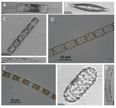
Figure 1: A mosaic of images of diatoms taken with a light microscope ($D$ & $E$) or an Imaging Flow cytomter ($A$, $B$, $C$, $F$ & $G$). A. Ditylum brightwellii B. Navicula sp. C. Chaetoceros sp. (a chain forming diatom), D. Lauderia annulata (a chain forming diatom), E. Lithodesmium undulatum (a chain forming diatom), F. Chorethron sp., and G. Cylindrotheca sp.

Particle inertia is most commonly predicted by the Stokes number $St$ which defines the relative timescale it takes a particle to respond to a change in the flow compared to the timescale at which the flow itself changes. The bulk of the literature is for $1\leq St\leq 10$, while $St$ values for phytoplankton are $3$ to $4$ orders of magnitude smaller. $St$ by itself, however, may not be a good predictor of particle behavior (Lucci et al., 2011; Fornari et al., 2016). In addition to $St$, settling velocities, can play an important role, describing the particle behavior in turbulence flows.

Conclusions from literature on cloud drops, oil droplets and aerosol do not transfer well to phytoplankton-like particles because of the difference in velocities, densities and size ratios (Wang & Maxey, 1993; Toschi & Bodenschatz, 2009; Gustavsson et al., 2014; Bec et al., 2014), therefore there is a clear need to extend modelling efforts to the parameter space at which phytoplankton operate. A parameter space for modelling phytoplankton is given in more detail in appendix A.

Another motivation for this study is to investigate the effect of shape on the dynamics of phytoplankton-like particles. So far only few studies have considered non-spherical particles in turbulent flows (Ni et al., 2015; Byron et al., 2015; Parsa & Voth, 2014). Phytoplankton exhibits a striking diversity of cell shapes and characteristics, which may influence their kinematics in important ways. For example, Durham et al. (2011) showed that spherical phytoplankton cells that are bottom-heavy and swim upwards (gyrotactic swimmers) tend to get trapped and cluster at regions with high shear gradients in a vortical flow field and are more likely to be found in down-welling regions of turbulent flows (Durham et al., 2013). This tendency to cluster, however, appears to be sensitive to the shape of cells (Zhan et al., 2014; Gustavsson et al., 2016). We are not aware of similar studies on the effect of the cell shape for settling, non-motile phytoplankton.

Here we use analytical and direct numerical simulations to examine the behavior of chain-forming diatoms in a turbulent flow. We focus on diatoms because this group is both ecologically important and promises diverse kinematics due to their relatively large size and diverse morphologies (e.g. Figure 1). Regarding their ecological importance, diatoms often dominate primary production in seasonal blooms and are considered key players in the biological pump that removes carbon from the surface layer that is in contact with the atmosphere to the deep ocean. Regarding their size and morphology, although unicellular, many species form colonies in the form of long chains that can reach up to a few $mm$ in size. Furthermore, diatoms have biomineralized siliceous cell walls that contribute a significant, and variable, excess density of cells. The behavior of these cells in a simple, steady shear flow has been studied in the lab (Karp-Boss & Jumars, 1998). While diatoms morphologies are complex and may include spines and other projections, as shown in figure 1, Nguyen et al. (2011) showed that in a simple shear flow the motion of a diatom with spines or projections could be well predicted from theory of the motion of spheroids in a simple shear flow, providing that the cell is described by the smallest inscribing spheroid that encompasses both the cell and its spines. We therefore model diatom chains as prolate spheroids.

We begin by introducing the kinematic and dynamic models, used in this study to describe the particle motion in §2. We compare the models and validate our numerical code in §3. Next, we examine whether turbulence affects sinking velocities and clustering of weakly inertial prolate spheroids and how it may vary as a function of different particle parameters (§4). Alteration of sinking velocities is explained further in this section, considering a simple shear flow. The main conclusions and final remarks are drawn in §5.

2 Governing equations and numerical method

2.1 Fluid phase

The incompressible turbulent velocity field, u, obeys the Navier-Stokes and continuity equations:

$$\frac{\partial\textbf{u}}{\partial t}+\textbf{u}\cdot\nabla\textbf{u} = -\nabla p+\frac{1}{Re}\nabla^{2}\textbf{u}+\textbf{f}\,,$$ (1)

$$\nabla\cdot\textbf{u} = \,0\,.$$ (2)

Here $t$ denotes the time, $p$ the pressure, $Re$ the Reynolds number and f the random forcing field necessary to maintain the turbulent velocity in a statistically steady state. The equations are discretized in a cubic domain with periodic conditions at the boundaries. We employ Direct Numerical Simulation (DNS) to solve all the relevant flow scales without any artificial model at the smallest scales. Since we evolve the equations in a three-periodic domain, it is natural to do so in Fourier space with a pseudo-spectral method. In this numerical scheme the nonlinear terms are evaluated in physical space using the classic $2/3$ rule to minimize aliasing error. Time integration is performed with a third-order low-storage Runge-Kutta method where the diffusive terms are analytically calculated while an Adam-Bashforth-like approximation is employed for the nonlinear terms (Rogallo, 1981). The stochastic forcing is evaluated in Fourier space and acts isotropically on the first shell of wave vectors. The forcing amplitude is constant in time and the field is delta-correlated in time and uniformly distributed in phase and directions (Vincent & Meneguzzi, 1994). We employed a resolution of $128^{3}$ grid points with a Taylor Reynolds number $Re_{\lambda}=100$ and $64^{3}$ grid points with a Taylor Reynolds number $Re_{\lambda}=60$. The turbulence is characterized by the Taylor Reynolds number $Re_{\lambda}\equiv u^{\prime}\lambda/\nu$, where $u^{\prime}$ is the root-mean-square of velocity fluctuations, $\nu$ is the kinematic viscosity and $\lambda$ is the Taylor microscale, $\lambda\equiv\sqrt{\epsilon/15\nu u^{\prime\,2}}$, with $\epsilon$ the kinetic energy dissipation rate. The resolution was chosen so that the velocity gradients are well resolved since they drive the the equation of motion of the particles. Particle statistics are computed from independent samples separated by $1.6$ turbulent Kolmogorov time scales, $\tau_{f}\equiv\sqrt{\nu/\epsilon}$, corresponding to about $300$ configurations per particle. The numerical code has been already employed to study gyrotactic micro-organisms in homogeneous turbulence (Zhan et al., 2014) and rain droplet evaporation in clouds (Sardina et al., 2015).

2.2 Solution of the particle motion

Two different approaches are adopted to evaluate the dynamics of sedimenting spheroids in a Lagrangian framework. Diatoms are typically smaller than the characteristic Kolmogorov scale in the upper mixed layer of the ocean (see appendix A) and so are the particles in our model. The flow properties at the particle position are evaluated via linear interpolation from the neighbouring grid points.

2.2.1 Method I - Kinematic model

Given the parameters relevant to plankton dynamics, the first approach assumes that the cells behave like passive tracers with a correction given by their Stokes settling velocity. The particle translational motion obeys

$$\frac{\mathrm{d}\textbf{x}}{\mathrm{d}t}=\textbf{u}|_{\mathrm{x}}+\textbf{v}_{s}\,(\textbf{p})\,,$$ (3)

$$\textbf{v}_{s}\,(\textbf{p})=v_{s}^{min}\hat{\textbf{e}}_{g}+\left(v_{s}^{max}-v_{s}^{min}\right)\left(\hat{\textbf{e}}_{g}\cdot\textbf{p}\right)\,\textbf{p}\,,$$ (4)

with x denoting spheroid position, $\textbf{u}|_{\mathrm{x}}$ the fluid velocity at spheroid position, p the spheroid orientation vector, $\textbf{v}_{s}$ the Stokes settling velocity and $\hat{\textbf{e}}_{g}$ a unit vector in the direction of gravity. $v_{s}^{min}$ and $v_{s}^{max}$ are the minimum and maximum settling speeds in quiescent flow, corresponding to the particles falling with their broad side perpendicular or parallel to the gravity direction. These velocities can be written as

$$v_{s}^{max}=\frac{\left(\rho_{p}-\rho_{f}\right)gl^{2}}{\mu_{f}}\gamma_{0}\left(\mathcal{AR}\right)\,\,\,\,;\,\,\,\,v_{s}^{min}=\frac{\left(\rho_{p}-\rho_{f}\right)gl^{2}}{\mu_{f}}\gamma_{1}\left(\mathcal{AR}\right)\,,$$ (5)

with $g$ the gravitational acceleration, $l$ the length of the spheroid’s major axis, $\mu_{f}$ the dynamic viscosity of the fluid, and $\rho_{p}$ and $\rho_{f}$ the densities of the particle and the fluid respectively. $\gamma_{0}$ and $\gamma_{1}$ are functions of the aspect ratio $\mathcal{AR}$, whose full expression can be found in Dahlkild (2011) among others. $\mathcal{AR}$ is defined as the ratio of polar over equatorial radii of the spheroid.

The spheroid rotation follows the inertialess Jeffery equation

$$\frac{\mathrm{d}\textbf{p}}{\mathrm{d}t}=\frac{1}{2}\,\boldsymbol{\omega}|_{\mathrm{x}}\times\textbf{p}+\alpha\left[\textbf{I}-\textbf{p}\textbf{p}\right]\cdot\textbf{E}|_{\mathrm{x}}\cdot\textbf{p}\,,$$ (6)

with $\boldsymbol{\omega}|_{\mathrm{x}}$ the flow vorticity at the particle’s position, I the second order identity tensor, $\textbf{E}|_{\mathrm{x}}$ the symmetric part of the velocity deformation tensor and $\alpha$ a function of the spheroid aspect ratio $\mathcal{AR}$, defined as

$$\alpha=\frac{\mathcal{AR}^{2}-1}{\mathcal{AR}^{2}+1}\,.$$ (7)

The same Runge-Kutta scheme used for the carrier phase is used to perform the time integration for equation 6. This is evaluated via a formulation based on quaternions. We evolve a total of $200000$ spheroids for each simulation.

2.2.2 Method II - Dynamic model

In the second approach, the spheroids are assumed to be inertial. They are assumed to obey the classic Maxey-Riley equation with an orientation correction for the Stokes drag (Gallily & Cohen, 1979; Brenner, 1964; Marchioli et al., 2014), without the Basset contribution:

$$\frac{\mathrm{d}\textbf{v}}{\mathrm{d}t}=\textbf{A}^{t}\textbf{K}^{\prime}\textbf{A}\frac{\textbf{u}-\textbf{v}}{\tau_{p}}+\frac{\rho_{f}}{\rho_{p}}\frac{\mathrm{D}\textbf{u}}{\mathrm{D}t}+\frac{1}{2}\frac{\rho_{f}}{\rho_{p}}\left[\frac{\mathrm{D}\textbf{u}}{\mathrm{D}t}-\frac{\mathrm{d}\textbf{v}}{\mathrm{d}t}\right]+\left(1-\frac{\rho_{f}}{\rho_{p}}\right)\textbf{g}\,,$$ (8)

$$\frac{\mathrm{d}\textbf{x}}{\mathrm{d}t}=\textbf{v}\,,$$ (9)

where the terms on the right-hand-side of equation 8 represent from left to right: the Stokes drag, the pressure gradient, added mass and lastly gravity (also accounting for the buoyancy force). The Basset history term is neglected in the present work due to its small contribution to the particle acceleration in the range of Stokes number and density ratio studied here (table 1) (see Olivieri, 2013; Olivieri et al., 2014; Daitche, 2015). In the expression above, v is the particle velocity, A is the transformation tensor between the fixed and the local spheroid reference frames, $*^{t}$ denotes the transpose operator, and $\tau_{p}$ the relaxation time for prolate spheroids, defined by

$$\tau_{p}=\frac{2\rho_{p}a^{2}}{9\mu_{f}}\,\,\frac{\mathcal{AR}\ln(\mathcal{AR}+\sqrt{\mathcal{AR}^{2}-1})}{\sqrt{\mathcal{AR}^{2}-1}}\,,$$ (10)

with $a$ the semi-minor axis of the prolate spheroid. $D*/Dt$ is the fluid material derivative, g the gravity vector. $\textbf{K}^{\prime}$ is the resistance second order tensor in the spheroid reference frame; it is a diagonal tensor of components, in which $z$ denotes the polar axis.

$$K^{\prime}_{xx}=K^{\prime}_{yy}=\frac{(16/6)(\mathcal{AR}^{2}-1)\ln(\mathcal{AR}+\sqrt{\mathcal{AR}^{2}-1})}{(2\mathcal{AR}^{2}-3)\ln(\mathcal{AR}+\sqrt{\mathcal{AR}^{2}-1})+\mathcal{AR}\sqrt{\mathcal{AR}^{2}-1}}\,,$$ (11)

$$K^{\prime}_{zz}=\frac{(8/6)(\mathcal{AR}^{2}-1)\ln(\mathcal{AR}+\sqrt{\mathcal{AR}^{2}-1})}{(2\mathcal{AR}^{2}-1)\ln(\mathcal{AR}+\sqrt{\mathcal{AR}^{2}-1})-\mathcal{AR}\sqrt{\mathcal{AR}^{2}-1}}\,.$$ (12)

The modified Maxey-Riley equation (8) is re-written in terms of relative velocity $\textbf{w}=\textbf{v}-\textbf{u}$ for a more accurate numerical solution,

$$\left(1+\frac{1}{2}\frac{\rho_{f}}{\rho_{p}}\right)\frac{\mathrm{d}\textbf{w}}{\mathrm{d}t}=-\textbf{A}^{t}\textbf{K}^{\prime}\textbf{A}\frac{\textbf{w}}{\tau_{p}}+\left(\frac{\rho_{f}}{\rho_{p}}-1\right)\frac{\mathrm{d}\textbf{u}}{\mathrm{d}t}-\frac{3}{2}\frac{\rho_{f}}{\rho_{p}}\textbf{w}\cdot\nabla\textbf{u}+\left(1-\frac{\rho_{f}}{\rho_{p}}\right)\textbf{g}\,,$$ (13)

and is advanced in time with an implicit predictor-corrector scheme to avoid numerical instabilities associated with the small values of the spheroid relaxation time.

The spheroid rotation is governed by the following equation

$$\frac{\mathrm{d}\left(\textbf{I}^{\prime}\cdot\boldsymbol{\omega}^{\prime}\right)}{\mathrm{d}t}\,+\,\boldsymbol{\omega}^{\prime}\times\left(\textbf{I}^{\prime}\cdot\boldsymbol{\omega}^{\prime}\right)=\textbf{N}^{\prime}\,,$$ (14)

with $\textbf{I}^{\prime}$ the spheroid moment of inertia tensor, $\boldsymbol{\omega}^{\prime}$ the spheroid angular velocity and $\textbf{N}^{\prime}$ the rotation torque, where the superscript $*^{\prime}$ denotes quantities in the spheroid reference frame. $\textbf{N}^{\prime}$ is given by

$$N^{\prime}_{x} = C_{x}\left[\left(1-\mathcal{AR}^{2}\right)E^{\prime}_{yz}+\left(1+\mathcal{AR}^{2}\right)\left(\Omega^{\prime}_{x}-\omega^{\prime}_{x}\right)\right]\,\,;\,\,C_{x}=\frac{16\pi\mu_{f}a^{3}\mathcal{AR}}{3\left(\beta_{0}+\mathcal{AR}^{2}\gamma_{0}\right)}\,,$$ (15)

$$N^{\prime}_{y} = C_{y}\left[\left(1-\mathcal{AR}^{2}\right)E^{\prime}_{xz}+\left(1+\mathcal{AR}^{2}\right)\left(\Omega^{\prime}_{y}-\omega^{\prime}_{y}\right)\right]\,\,;\,\,C_{y}=\frac{16\pi\mu_{f}a^{3}\mathcal{AR}}{3\left(\beta_{0}+\mathcal{AR}^{2}\gamma_{0}\right)}\,,$$ (16)

$$N^{\prime}_{z} = C_{z}\left(\Omega^{\prime}_{z}-\omega^{\prime}_{z}\right)\,\,;\,\,C_{z}=\frac{32\pi\mu_{f}a^{3}\mathcal{AR}}{3\left(\alpha_{0}+\beta_{0}\right)}\,,$$ (17)

with ${\bf\Omega}^{\prime}$ is the fluid rate of rotation tensor, and $\alpha_{0}$, $\beta_{0}$ and $\gamma_{0}$ are coefficient functions of the aspect ratio whose expression can be found in Jeffery (1922).

3 Validation and comparison between the two models

We first compare the two models to assess whether the simpler, inertialess model can be used for simulations aiming to study the settling of plankton in turbulent flow (see table 2). For each method, we perform two simulations at $Re_{\lambda}$ around $60$ and spheroid aspect ratio of $\mathcal{AR}=5$ . The two cases differ in the choice of density ratio ($1.3$ in figure 2 and $1.05$ in figure 3) and average settling velocity ($2.3u_{\eta}$ in figure 2 and $1.1u_{\eta}$ in figure 3).

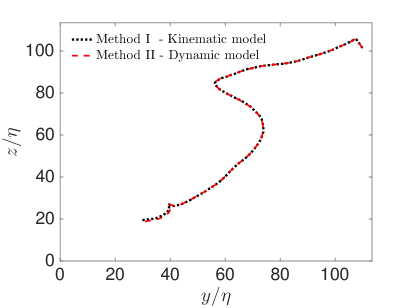
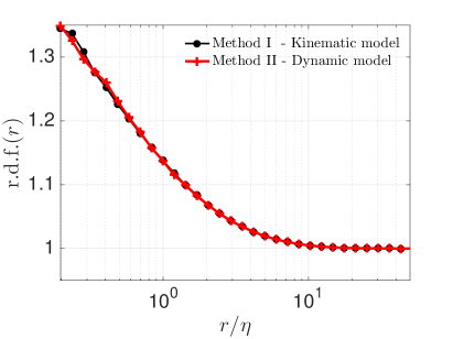
Figure 2: Comparison between kinematic (non-inertial; black line) and dynamic (inertial; red line) models: $(a)$ Example trajectories of the two particles, using the two models from $t=0$ to $t=40\tau_{\eta}$ and $(b)$ radial distribution function (r.d.f) of particle position. $Re_{\lambda}=60$ ; $\mathcal{AR}=5$ ; $\rho_{p}/\rho_{f}=1.3$ ; $v^{iso}_{s}\approx 2.3u_{\eta}$. $v^{iso}_{s}$ is the average settling speed for spheroids in a quiescent flow and the r.d.f measures the probability to find a particle pair at a given radial distance, normalized by the values of a uniform distribution. (see § 4 for the formulation of r.d.f. and $v^{iso}_{s}$).

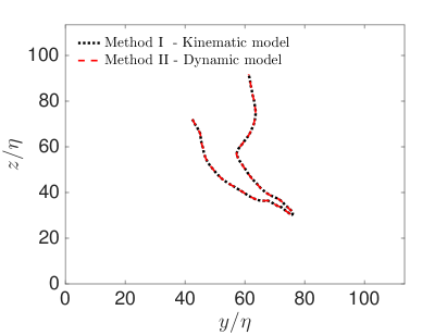
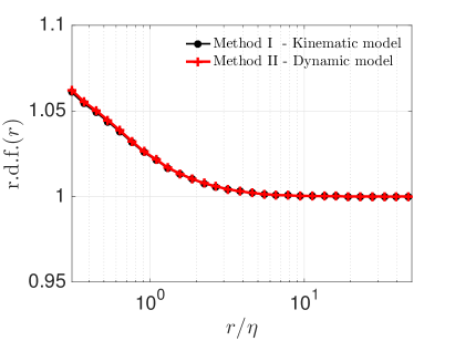
Figure 3: Comparison between kinematic (non-inertial; black line) and dynamic (inertial; red line) models: $(a)$ Example trajectories of the two particles, using the two models from $t=0$ to $t=40\tau_{\eta}$ and $(b)$ radial distribution function (r.d.f) of particle position. $Re_{\lambda}=60$ ; $\mathcal{AR}=5$ ; $\rho_{p}/\rho_{f}=1.05$ ; $v^{iso}_{s}\approx 1.1u_{\eta}$. $v^{iso}_{s}$ is the average settling speed for spheroids in a quiescent flow and the r.d.f measures the probability to find a particle pair at a given radial distance, normalized by the values of a uniform distribution. (see § 4 for the formulation of r.d.f. and $v^{iso}_{s}$).

We consider both particle trajectories and statistical properties: the two different methods provide the same result for both the single spheroid trajectories (panels $(a)$ of figures 2 and 3) and the global spheroid two-point distribution function (panels $(b)$ of figures 2 and 3). As seen in these figures, in the limit of small density ratio and relaxation time the two models provide the same dynamics. Therefore, we have used the non-inertial tracer (kinematic) model for the simulations at higher Reynolds number that will be described in the next sections.

4 Results

$\mathcal{AR}$	$1$	$2$	$3$	$5$	$10$	$20$
$v_{s}^{max}$	$3.03$	$3.17$	$3.11$	$2.90$	$2.46$	$1.97$
$v_{s}^{min}$	$3.03$	$2.77$	$2.53$	$2.18$	$1.71$	$1.29$
$v_{s}^{max}/v_{s}^{min}$	$1$	$1.14$	$1.23$	$1.33$	$1.44$	$1.53$
$v^{iso}_{s}$	$3.03$	$2.90$	$2.72$	$2.42$	$1.96$	$1.52$

Table 1: Maximum, minimum and average of settling velocities in quiescent flow, scaled with the Kolmogorov velocity for the investigated cases with different aspect ratios. $\rho_{p}/\rho_{f}=1.05$ and $D_{eq}=\eta/6$.

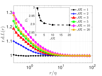
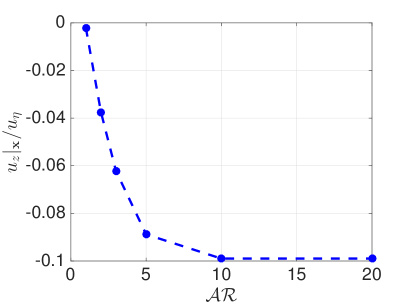
Figure 4: $(a)$ Radial distribution function of particle positions; the inset in this panel reports the fractal dimension of the clustering, estimated by fitting r.d.f. with a power-law in the range $r/\eta=[0.2:2]$, $(b)$ average of fluid vertical velocity at the particle position and $(c)$ increase in the settling velocity (difference in the settling rate with respect to the quiescent settling average $v^{iso}_{s}$, normalized by $v^{iso}_{s}$).

We first investigate the settling of prolate spheroidal particles of constant volume, focusing on the effect of the particle aspect ratio. The parameters used are $Re_{\lambda}=100$, $\frac{\rho_{p}}{\rho_{f}}=1.05$ and $D_{eq}=\eta/6$ where $D_{eq}$ is the diameter of a sphere having the same volume as the prolate spheroid. Fixing the volume, the settling speed varies with the aspect ratio. It should be noted that for the higher aspect ratio cases ($\mathcal{AR}\geq 15$), examined here, the larger diameter of the spheroid exceeds Kolmogorov length scale $\eta$ ($\approx 1.24$ for $\mathcal{AR}=24$). This barely affects the results since rods act as tracers when their length is less than $5\eta$ and deviations from tracer behavior are very small until about $15\eta$ (Parsa & Voth, 2014). For the simulations presented here, the average settling speed of an uniformly distributed suspension, $v^{iso}_{s}$, varies in the range $1.5-3u_{\eta}$. Table 1 shows the settling velocities for the investigated cases. The reported values are all normalized by the Kolmogorov velocity. Note that the average settling speed $v^{iso}_{s}$ for spheroids in a quiescent flow is calculated as:

$$v^{iso}_{s}=\frac{\left(v^{max}_{s}+2v^{min}_{s}\right)}{3}\,,$$ (18)

based on the assumption that the orientation of spheroids (cosine of the angle between spheroid’s symmetric axis and the gravity direction) are uniformly distributed.

The results are shown in figure 4. The main observation is that within the parameter space relevant to diatom chains, settling spheroids weakly cluster (figure 4 panel a) and preferentially sample regions of down-welling flow, leading to downward velocity biases of up to $10\%$ of the Kolmogorov velocity $u_{\eta}$ (figure 4 panel b). This corresponds to an increase of the mean settling speed of about $5\%$ compared to the mean settling speed in quiescent fluid (panel c in figure 4). These effects increase with the aspect ratio, $\mathcal{AR}$, and saturate for $\mathcal{AR}\geq 10$.

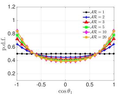
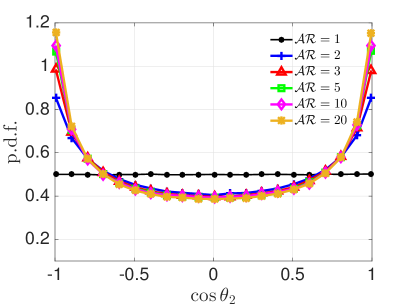
Figure 5: p.d.f of orientation of particles with different aspect ratios with respect to the three eigenvectors of the deformation tensor $(a-c)$ and $(d)$ the local vorticity vector.

To quantify patchiness (clustering) in fully three-dimensional isotropic turbulent flows, we use the radial pair distribution function (RDF), sometimes also called the correlation function. The RDF measures the probability of finding a particle pair separated by a given radial distance, normalized by the value expected from a uniform distribution. This is defined as

$$g\left(r\right)=\frac{1}{4\pi r^{2}}\frac{dN_{r}}{dr}\frac{1}{n_{0}},$$ (19)

where, $n_{0}=0.5N_{p}\left(N_{p}-1\right)/V_{0}$ is the density of pairs in the whole volume $V_{0}$. $N_{p}$ is the total number of particles in the domain and $N_{r}$ is the number of pairs at distance $r$. The small volume fraction, used here, removes the exclusion effects, and thus an RDF for a random distribution results in a flat value of $1$. The radial distribution function (RDF) is reported in figure 4(a). In the inset of the same figure, we report the scaling exponent of RDF at small separations, also often used as an indicator of patchiness (Durham et al., 2013). This exponent denotes the fractal dimension of the set where particles are found. Patchiness is seen to increase with the particle aspect ratio and saturate at the largest values considered.

In figure 5, we study the relation between particle orientation and the underlying flow field when varying the particle shape. In figure 5(a), (b) and (c), we show the orientation of the particle with respect to the three eigendirections of the strain tensor, defined such that $\lambda_{1}>\lambda_{2}>\lambda_{3}$ so that the first eigendirection is extensional and the third eigendirection is compressional. The angles between the eigendirections and the spheroid orientation are denoted as $\theta_{1}$, $\theta_{2}$ and $\theta_{3}$. In figure 5d, we show $\psi$, the angle between the orientation and the local vorticity vector. While spherical particles, $\mathcal{AR}=1$, are isotropic in nature, elongated spheroids tend to align with the local flow strain, more frequently with the second eigendirection, and with the local flow vorticity. Indeed, the pdfs peak when prolate particles are parallel to the eigendirections associated with $\lambda_{2}$ and $\lambda_{1}$. An increasing probability of parallel alignment with the first two eigendirections of the strain is seen with increased aspect ratio. The spheroid is most likely to be normal to the third eigendirection of the strain as shown in figure 5(c). The strongest tendency to align with the local vorticity vector is consistent with previous observations for neutrally buoyant spheroids (Chevillard & Meneveau, 2013; Ni et al., 2015). The alignment with the vorticity vector increases with the aspect ratio $\mathcal{AR}$.

4.1 Numerical experiments

To understand how the observed increase of settling speed and preferential sampling depends on the different governing parameters, we perform a series of numerical experiments in order to investigate the effect of the aspect ratio, $\mathcal{AR}$, the amplitude of the sedimenting velocity $v^{iso}_{s}$ and the ratio between the maximum (spheroid aligned with the gravity direction) and minimum (normal to gravity) settling speed $v_{s}^{max}/v_{s}^{min}$. In each series of simulations we fix all the parameters except for one to focus on a single parameter effect. While varying only one parameter can result in unrealistic conditions occasionally, it sheds light on the isolated effect of the parameter of interest on particles’ collective behavior. As mentioned above, the non-inertial (kinematic) model is used in these simulations.

4.1.1 Effect of sedimenting velocity magnitude

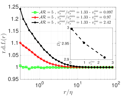
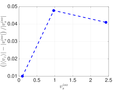
Figure 6: $(a)$ Radial distribution function of particle positions and $(b)$ increase in the settling velocity for $\mathcal{AR}=5$ and the indicated values of $v_{s}^{iso}$.

First we examine how particle clustering varies with the amplitude of the settling speed. To this end, we keep the aspect ratio $\mathcal{AR}=5$, corresponding to a ratio between maximum and minimum settling speed, $v_{s}^{max}/v_{s}^{min}=1.33$, and change $v_{s}^{iso}$ from 0.1 to about 2.5 Kolmogorov velocities (this may correspond to a change in the particle size with respect to the turbulence Kolmogorov scale or a change in particle density). Results in figure 6(a) show that patchiness increases with the average settling speed, as measured by the RDF or by the fractal dimension (inset in figure 6(a)). The increased clustering, however, does not correspond to an increase of the relative average settling speed when $v_{s}^{iso}$ is greater than the Kolmogorov velocity.

4.1.2 Effect of aspect ratio

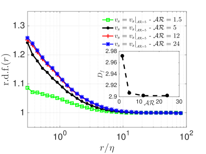
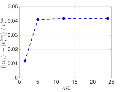
Figure 7: $(a)$ Radial distribution function of particle positions and $(b)$ increase in the settling velocity for the different aspect ratios indicated, while keeping the same maximum and minimum settling speed.

To elucidate the role of the particle rotation rate on the observed preferential sampling, we vary $\mathcal{AR}$, while artificially keeping the settling speed fixed, both the components parallel and normal to gravity, fixed at values corresponding to $AR=5$ in table 1. The solution of Jeffery’s equation (6) reveals that the time spent aligned with the local shear increases with increasing aspect ratio. The results, displayed in figure 7, show that the RDF and the relative increase of sedimenting velocity saturate for $\mathcal{AR}\geq 5$. Interestingly, rotation rates of oblate and prolate particles are seen to saturate for $\mathcal{AR}>5$ and for $\mathcal{AR}<1/5$ in the study of Byron et al. (2015). We have also observed, not shown here, that the alignment with the local vorticity increases with the aspect ratio and saturates when $\mathcal{AR}\geq 5$ unlike the cases in figure 5, where it continues to increase; this suggests that the alignment with vorticity is influenced by the difference between settling parallel and normal to gravity, which is fixed here.

4.1.3 Effect of local alignment

To show the isolated effect of particle alignment with the local vorticity vector we performed a simulation, forcing the elongated spheroid to be always aligned with the local vorticity (figure 8): we observe that clustering decreases in this case, relative to the case of in which the particle was free to rotate, and therefore clustering cannot be explained by the alignment with the local flow vorticity.

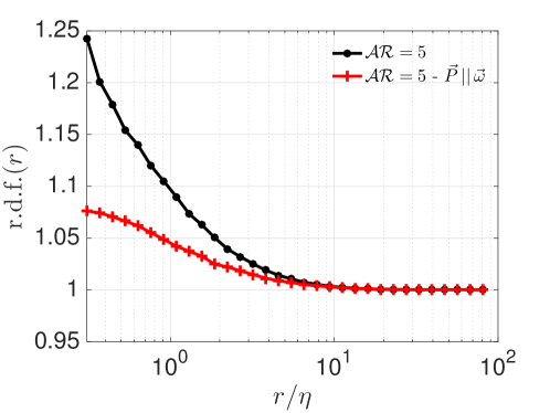
Figure 8: Radial distribution function of particle positions for particles with $\mathcal{AR}=5$ and particles with the same sedimenting velocity but with their orientation forced to be always aligned with the local vorticity vector.

4.1.4 Effect of drag anisotropy

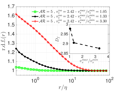
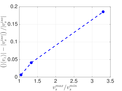
Figure 9: $(a)$ Radial distribution function of particle positions and $(b)$ increase in the settling velocity for settling spheroids with aspect ratio $\mathcal{AR}=5$, fixed average settling speed $v_{s}^{iso}=2.42$ and different ratios between settling speed in the direction normal and parallel to gravity, $v_{s}^{max}/v_{s}^{min}$, as indicated in the legend.

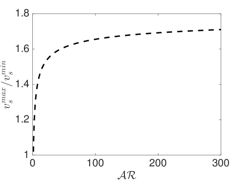
Figure 10: $v_{s}^{max}/v_{s}^{min}$ versus $\mathcal{AR}$ for prolate particles, see e.g.  analytical expressions reported in Dahlkild (2011).

One important feature of non-spherical particles in inertialess flows is their drag anisotropy, which can also be exploited by micro-organisms for locomotion. In the case of settling prolate spheroids, this anisotropy is seen in the oblique settling of inclined particles and in the difference between settling speed when oriented parallel or normal to gravity. For the results presented so far we followed the analytical expression for the settling speed derived for prolate spheroids. Shapes in nature are, however, more complicated. Flexibility and non-uniformly distributed mass are likely to cause deviation from the idealized case. To understand more the relevance of drag anisotropy we perform simulations of spheroids with aspect ratio $\mathcal{AR}=5$ and fixed average settling speed $v_{s}^{iso}=2.42$, while varying the ratio between settling speed in the direction normal and parallel to gravity, $v_{s}^{max}/v_{s}^{min}$. As seen in figure 9(a) clustering increases significantly with drag anisotropy, or $v_{s}^{max}/v_{s}^{min}$. More interestingly, the relative settling speed increases by up to about $20\%$ when $v_{s}^{max}/v_{s}^{min}=3.3$. The value $3.3$ is chosen to artificially emphasize the drag anisotropy effect; however, note that the ratio between maximum and minimum settling speed of spheroidal particles increases with the aspect ratio and saturates at about $1.75$ (figure 10).

4.2 Mechanism for increased settling speed

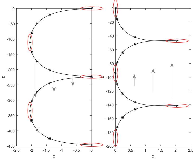
Figure 11: Trajectory of single particle in vertical laminar shear over a Jeffery orbit. Particle initially at the origin with orientation (a) $\theta=\pi/2$, (b) $\theta=0$. Stars indicate position at equally spaced time intervals, red ellipses indicate orientation of particle orientation. Grey arrows indicate flow velocity $\mathbf{u}=-\gamma x\hat{\mathbf{e}}_{g}$.

To understand why ellipsoidal particles preferentially locate in regions of down-welling flow and thus have an enhanced settling speed, we consider vertical linear shear, $\mathbf{u}=-\gamma x\hat{\mathbf{e}}_{g}$ with motion constrained to the $x-z$ plane. We define $\theta$ to be the angle the particle symmetry axis makes with the vertical, so that in $x-z$ co-ordinates the orientation vector is given by $\mathbf{p}=(\sin\theta,\cos\theta)^{T}$.

From Jeffery’s equation (6) the time evolution of particle orientation is given by

$$\dot{\theta}=\frac{\gamma}{2}\left(-1+\alpha\cos 2\theta\right).$$ (20)

Note that the particle rotates most slowly when $\theta=0$ or $\pi$, and thus spends more time in these states, i.e. aligned with the local shear. From equation (4), the vertical velocity of a particle is given by

$$v_{z}=\gamma x-v_{s}^{min}-\left(v_{s}^{max}-v_{s}^{min}\right)\cos^{2}\theta.$$

The time-averaged vertical velocity over a Jeffery orbit (of duration $T=4\pi/\gamma\sqrt{1-\alpha^{2}}$) is given by

$$\overline{v_{z}} = \frac{1}{T}\int_{0}^{T}(\gamma x-v_{s}^{min}-\left(v_{s}^{max}-v_{s}^{min}\right)\cos^{2}\theta)dt$$

$$= \gamma\overline{x}-v_{s}^{min}-\frac{\left(v_{s}^{max}-v_{s}^{min}\right)\sqrt{1-\alpha^{2}}}{2\pi}\int_{0}^{2\pi}\frac{\cos^{2}\theta}{-1+\alpha\cos 2\theta}d\theta,$$

where $\overline{x}$ is the time-averaged horizontal position. The effect of the shear strength, $\gamma$, only appears through the term $\gamma\overline{x}$, and so the effect of the shear on the total vertical velocity of particles can be determined if we know the time-averaged horizontal position. In particular, the only way cells are predicted to exhibit enhanced settling is if they spend more time in down-welling regions.

To demonstrate how the time-averaged horizontal position is biased towards down-welling regions, yielding enhanced settling, we numerically compute particle trajectories for a complete Jeffery orbit for an example set of parameters taken from table 1: $\gamma=1$, $\mathcal{AR}=20$ ($\alpha=0.995$), $v_{s}^{min}=1.29$ and $v_{s}^{max}=1.97$ (see figure 11). Particles are initially located at the origin, and the initial orientation is taken as $\theta=0$ or $\theta=\pi/2$. Particles initially horizontal ($\theta=\pi/2$, figure 11a) have a negative horizontal component due to shear-induced lift, causing them to translate into down-welling flow. As the particle rotates, it reaches a minimum horizontal position at the point when $\theta=0$ and then reverses its horizontal component of motion back towards $x=0$ which is attained when $\theta=3\pi/2$. The particle has a slowest rotation rate when $\theta=0$ or $\pi$ corresponding to the minimum horizontal position, and thus the time-averaged horizontal position is less than the midpoint of the horizontal limits of the trajectory. This bias represents a tendency to cluster in down-welling flow. Particles initially vertical ($\theta=0$, figure 11b) sediment with a positive horizontal component into upwelling flow. As the particle rotates, it reaches a maximum horizontal position at the point when $\theta=3\pi/2$ and then reverses its horizontal component of motion back towards $x=0$ which is attained when $\theta=\pi$. Again, the particle has a slowest rotation rate at the minimum horizontal position, and thus the time-averaged horizontal position is less than the midpoint of the horizontal limits of the trajectory. This simple example shows how shear, rotation, lift, and drag-anistropy couple to bias particle trajectories towards downward flow.

5 Final remarks

We report results from simulations of elongated, rigid particles (prolate spheroids) with different aspect ratios sinking in homogenous, isotropic turbulence. Parameters used in this study represent marine or freshwater diatoms that are characterized by very small relaxation times compared to that of the fluid but with high settling velocities on the order of Kolmogorov velocities. Given the small size of diatoms relative to the Kolmogorov length-scale and their short relaxation time, cells are assumed to behave like passive tracers with a correction given by their Stokes’ settling velocity. This assumption is confirmed by comparing with a dynamic model where Stokes’ drag, gradient pressure and added mass are taken into account. Results from these models show the same dynamics in the range of Stokes numbers and density ratios relevant to diatoms. We therefore use the kinematic (non-inertial tracer) model, which allows simpler control over different parameters, allowing us to study how and why turbulence affects sinking velocities and clustering of diatoms.

Ruiz et al. (2004) showed that turbulence increases the average sinking velocity of the diatom Coscinodiscus sp. in a laboratory set-up. They attributed their observations to preferential sampling of down-welling regions of the flow, a mechanism that was previously investigated for highly inertial particles with Stokes numbers that are several orders of magnitude larger than those of phytoplankton, and hypothesized that preferential sampling will also result in local clustering. Here we show numerically that preferential sampling occurs within the parameter space relevant to diatoms but only for non-spherical particles. Preferential sampling of down-welling flow results in local clustering of particles and a relative increase in settling velocity, but the effect on the latter is smaller ($\leq 5\%$), compared to the one shown in the lab (Ruiz et al., 2004). We provide further insight on the mechanism involved by showing that elongated spheroids tend to align with the local flow strain (more frequently with the second eigendirection) and with the local flow vorticity (this is in agreement with previous studies on neutrally buoyant spheroids in homogenous isotropic turbulence, Ni et al., 2015). To understand why ellipsoidal particles preferentially locate in regions of down-welling flow and thus have an enhanced settling speed, we consider a simple case of one particle sedimenting in linear shear flow. We demonstrate how the time-averaged (over a complete Jeffery orbit) horizontal position comes to be biased towards down-welling regions due to the interaction of orientation, shear, drag, and lift.

Cell shape is an important morphological trait affecting many aspects in the ecology of phytoplankton (Smayda, 1970; Lewis, 1976; Sournia, 1982; Reynolds, 1989; Reynolds & Irish, 1997; Karp-Boss & Boss, 2016) and results from our numerical model further highlight the complex interactions of cell shape with ambient flows. Interestingly, the observed increase in settling speeds does not increase indefinitely, and saturates for $\mathcal{AR}>10$. Increasing the aspect ratio, while keeping the particle volume and density ratio constant, varies other characteristics of the particle simultaneously. For example, the mean settling speed in quiescent flow decreases as the ratio between maximum (when particle is oriented parallel to the gravity direction) and minimum (when particle is oriented normal to the gravity direction) settling speed increases. We therefore perform a series of numerical experiments to isolate the effect of the aspect ratio $\mathcal{AR}$, the magnitude of settling velocity $v^{iso}_{s}$ and the ratio between the maximum and minimum settling speed $v_{s}^{max}/v_{s}^{min}$ in quiescent flow. When $v^{iso}_{s}$ and $v_{s}^{max}/v_{s}^{min}$ are held constant, the increase in clustering and settling speed begins to saturates at $\mathcal{AR}=5$. This indicates that the relative enhancement that we observe for ellipsoids with aspect ratios larger than $5$ is not due to a direct enhancement by the aspect ratio effect but due to an increase in the ratio between the maximum and minimum settling speed ($v_{s}^{max}/v_{s}^{min}$) that is associated with a change in particle shape ($\mathcal{AR}$, while volume remains constant). Interestingly, an analysis of typical aspect ratios among phytoplankton shows a peak in distribution at $\mathcal{AR}\sim 5$ (Clavano et al., 2007; Karp-Boss & Boss, 2016), but this may be a coincidence because in nature multiple processes (grazing, diffusion, mechanical breakage by shear) act simultaneously as selective pressures on shape and size in phytoplankton (Karp-Boss & Boss, 2016).

Spheroids with higher average Stokes settling speeds ($v^{iso}_{s}$) show greater tendency to cluster (Figure 6). However, when $v^{iso}_{s}$ is greater than Kolmogorov velocity, the increase in clustering does not correspond to an increase in relative average settling speed. Clustering increases significantly with drag anisotropy (i.e., the ratio $v_{s}^{max}/v_{s}^{min}$) in a way that does not appear to saturate. Drag anisotropy increases with increasing $\mathcal{AR}$ and forces the particles to sample regions of down-welling flow to a further extent, even when the isolated effect of aspect ratio is saturated.

Appendix A Parameter space for phytoplankton

00Parameter000000	0000Values
Kinetic energy dissipation rate ($\epsilon$)	0000000$10^{-10}$ - $10^{-4}\,m^{2}s^{-3}$
Taylor Reynolds number ($Re_{\lambda}$)	00000$50-200$
Sinking velocity of diatoms ($v_{s}^{iso}$)	0000000$2\,\mu m\,s^{-1}$ - $1\,mm\,s^{-1}$
Velocity ratio ($v_{s}^{iso}/u_{\eta}$)	00000$0.02$ - $11$
Size ratio ($L/\eta$)	00000$0.003$ - $2$
Density ratio ($\rho_{p}/\rho_{f}$)	0000$1$ - $1.3$
Relaxation time of a cell ($\tau_{p}$)	00000$\sim 10^{-4}\,s$
Relaxation time of fluid ($\tau_{f}$)	$\,\,\,\,\,\,\,\sim\,\,1\,s$
Stokes number ($\tau_{p}/\tau_{f}$)	00000$\sim 10^{-4}$

Table 2: A summary of the parameter values relevant to marine diatoms. The value of $\epsilon$ is considered $10^{-6}$ $m^{2}s^{-3}$ for calculating $\tau_{f}$ and $Re_{\lambda}$.

Dissipation rates of turbulent kinetic energy $\epsilon$ in the ocean vary greatly in space and time. In the open ocean, typical values range from $10^{-10}$ to $10^{-7}\,m^{2}s^{-3}$, while coastal regions, especially those influenced by tidal fronts, experience higher dissipation rates, on the order of $10^{-7}$ to $10^{-4}\,m^{2}s^{-3}$ (Smyth & Moum, 2000; Barton et al., 2014). Within the water column, turbulence kinetic energy dissipation rate are higher at the surface and decrease with depth (Smyth & Moum, 2000). Given the kinematic viscosity of seawater $\nu\sim 10^{-6}m^{2}s^{-1}$, characteristic Kolmogorov length scale $\eta$ in the ocean ranges from $\sim 300\,\mu m$ to a few $mm$. Generally speaking, diatoms are smaller than characteristic Kolmogorov length scales in the ocean, and range in size from a few $\mu m$ for small solitary cells to 100s of $\mu m$ in length for chain forming species (Karp-Boss & Jumars, 1998). This size ratio may become order $1$ for very long chains in strong turbulence but this would represent an extreme case. Sinking velocities of diatoms have been measured in quiescent water by measuring the temporal change in concentration of diatoms at the top and bottom of a water column with a known height and calculating average (community) settling velocities. Using this approach, settling velocities ($v_{s}^{iso}$) were found to range between $2\,\mu m\,s^{-1}$ to $\sim 1\,mm\,s^{-1}$ (reviewed in Smayda, 1970).

Characteristic velocities at dissipation scale in the ocean ($u_{\eta}=(\nu\epsilon)^{1/4}$) are in the order of $0.01$ - $0.1$ $mm\,s^{-1}$, resulting in velocity ratio $v_{s}^{iso}/u_{\eta}\approx$ $1$ - $4$ (assuming maximum $v_{s}^{iso}$ of $1\,mm\,s^{-1}$). Densities of marine diatoms $\rho_{p}$ have not been measured directly but estimated from Stokes equation for settling spheres, based on measured sinking velocities. Densities were found to be in the range of $1.03$ - $1.15$ $g\,cm^{-3}$ for actively growing cells with higher values for cells in senescence ($1.059$-$1.33$ $g\,cm^{-3}$; Eppley et al., 1967). Average density of surface seawater $\rho_{f}$ is $1.025$ $g\,cm^{-3}$ and thus the density ratio relevant to the parameter space of phytoplankton is in the range of $1$ - $1.3$. Table 2 summarizes the parameter values relevant to marine diatoms.

References

- Barry et al. (2015) Barry, M. T., Rusconi, R., Guasto, J. S. & Stocker, R. 2015 Shear-induced orientational dynamics and spatial heterogeneity in suspensions of motile phytoplankton. Journal of The Royal Society Interface 12 (112), 20150791.
- Barton et al. (2014) Barton, A. D., Ward, B. A., Williams, R. G. & Follows, M. J. 2014 The impact of fine-scale turbulence on phytoplankton community structure. Limnology and Oceanography: Fluids and Environments 4 (1), 34–49.
- Bec et al. (2014) Bec, J., Homann, H. & Ray, S. S. 2014 Gravity-driven enhancement of heavy particle clustering in turbulent flow. Physical review letters 112 (18), 184501.
- Brenner (1964) Brenner, H. 1964 The stokes resistance of an arbitrary particle iv arbitrary fields of flow. Chemical Engineering Science 19 (10), 703–727.
- Byron et al. (2015) Byron, M., Einarsson, J., Gustavsson, K., Voth, G., Mehlig, B. & Variano, E. 2015 Shape-dependence of particle rotation in isotropic turbulence. Physics of Fluids (1994-present) 27 (3), 035101.
- Chevillard & Meneveau (2013) Chevillard, L. & Meneveau, C. 2013 Orientation dynamics of small, triaxial–ellipsoidal particles in isotropic turbulence. Journal of Fluid Mechanics 737, 571–596.
- Clavano et al. (2007) Clavano, W. R., Boss, E. & Karp-Boss, L. 2007 Inherent optical properties of non-spherical marine-like particles from theory to observation. Oceanogr Mar Biol, Annu Rev 45, 1–38.
- Dahlkild (2011) Dahlkild, A. A. 2011 Finite wavelength selection for the linear instability of a suspension of settling spheroids. Journal of Fluid Mechanics 689, 183–202.
- Daitche (2015) Daitche, A. 2015 On the role of the history force for inertial particles in turbulence. Journal of Fluid Mechanics 782, 567–593.
- Denny (1993) Denny, M. W. 1993 Air and water: the biology and physics of life’s media. Princeton University Press.
- Durham et al. (2013) Durham, W. M., Climent, E., Barry, M., De Lillo, F., Boffetta, G., Cencini, M. & Stocker, R. 2013 Turbulence drives microscale patches of motile phytoplankton. Nature communications 4.
- Durham et al. (2011) Durham, W. M., Climent, E. & Stocker, R. 2011 Gyrotaxis in a steady vortical flow. Physical Review Letters 106 (23), 238102.
- Eppley et al. (1967) Eppley, R. W., Holmes, R. W. & Strickland, J. D. H. 1967 Sinking rates of marine phytoplankton measured with a fluorometer. Journal of Experimental Marine Biology and Ecology 1 (2), 191–208.
- Fornari et al. (2016) Fornari, W., Picano, F. & Brandt, L. 2016 Sedimentation of finite-size spheres in quiescent and turbulent environments. Journal of Fluid Mechanics 788, 640–669.
- Gallily & Cohen (1979) Gallily, I. & Cohen, A. H. 1979 On the orderly nature of the motion of nonspherical aerosol particles. ii. inertial collision between a spherical large droplet and an axially symmetrical elongated particle. Journal of Colloid and Interface Science 68 (2), 338–356.
- Guazzelli & Morris (2011) Guazzelli, E. & Morris, J. F. 2011 A physical introduction to suspension dynamics, , vol. 45. Cambridge University Press.
- Gustavsson et al. (2016) Gustavsson, K., Berglund, F., Jonsson, P. R. & Mehlig, B. 2016 Preferential sampling and small-scale clustering of gyrotactic microswimmers in turbulence. Physical review letters 116 (10), 108104.
- Gustavsson et al. (2014) Gustavsson, K., Vajedi, S. & Mehlig, B. 2014 Clustering of particles falling in a turbulent flow. Physical Review Letters 112 (21), 214501.
- Jeffery (1922) Jeffery, G. B. 1922 The motion of ellipsoidal particles immersed in a viscous fluid. In Proceedings of the Royal Society of London A: Mathematical, Physical and Engineering Sciences, , vol. 102, pp. 161–179. The Royal Society.
- Karp-Boss & Boss (2016) Karp-Boss, L. & Boss, E. 2016 The elongated, the squat and the spherical: Selective pressures for phytoplankton shape. In Aquatic Microbial Ecology and Biogeochemistry: A Dual Perspective, pp. 25–34. Springer.
- Karp-Boss & Jumars (1998) Karp-Boss, L. & Jumars, P. A. 1998 Motion of diatom chains in steady shear flow. OCEANOGRAPHY 43 (8).
- Kiørboe (2008) Kiørboe, T. 2008 A mechanistic approach to plankton ecology. Princeton University Press.
- Lazier & Mann (1989) Lazier, J. R. N. & Mann, K. H. 1989 Turbulence and the diffusive layers around small organisms. Deep Sea Research Part A. Oceanographic Research Papers 36 (11), 1721–1733.
- Lewis (1976) Lewis, W. M. 1976 Surface/volume ratio: implications for phytoplankton morphology. Science 192 (4242), 885–887.
- Lucci et al. (2011) Lucci, F., Ferrante, A. & Elghobashi, S. 2011 Is stokes number an appropriate indicator for turbulence modulation by particles of taylor-length-scale size? Physics of Fluids (1994-present) 23 (2), 025101.
- Marchioli et al. (2014) Marchioli, C., Zhao, L. & Andersson, H. I. 2014 On the relative rotational motion between rigid fibers and fluid in turbulent channel flow. Physics of Fluids (1994-present) 28 (1), 013301.
- Maxey (1987) Maxey, M. R. 1987 The gravitational settling of aerosol particles in homogeneous turbulence and random flow fields. Journal of Fluid Mechanics 174, 441–465.
- Murray (1970) Murray, S. P. 1970 Settling velocities and vertical diffusion of particles in turbulent water. Journal of geophysical research 75 (9), 1647–1654.
- Nguyen et al. (2011) Nguyen, H., Karp-Boss, L., Jumars, P. A & Fauci, L. 2011 Hydrodynamic effects of spines: A different spin. Limnology and Oceanography: Fluids and Environments 1 (1), 110–119.
- Ni et al. (2015) Ni, R., Kramel, S., Ouellette, N. T & Voth, G. A. 2015 Measurements of the coupling between the tumbling of rods and the velocity gradient tensor in turbulence. Journal of Fluid Mechanics 766, 202–225.
- Nielsen (1993) Nielsen, P. 1993 Turbulence effects on the settling of suspended particles. Journal of Sedimentary Research 63 (5).
- Nielsen (2007) Nielsen, P. 2007 Mean and variance of the velocity of solid particles in turbulence. In Particle-Laden Flow, pp. 385–391. Springer.
- Olivieri (2013) Olivieri, S. 2013 Analysis of the forces acting on particles in homogeneous isotropic turbulence.
- Olivieri et al. (2014) Olivieri, S., Picano, F., Sardina, G., Ludicone, D. & Brandt, L. 2014 The effect of the basset history force on particle clustering in homogeneous and isotropic turbulence. Physics of Fluids (1994-present) 26 (4), 041704.
- Parsa & Voth (2014) Parsa, S. & Voth, G. A. 2014 Inertial range scaling in rotations of long rods in turbulence. Physical review letters 112 (2), 024501.
- Reynolds (1989) Reynolds, C. S. 1989 Physical determinants of phytoplankton succession. In Plankton ecology, pp. 9–56. Springer.
- Reynolds & Irish (1997) Reynolds, C. S. & Irish, A. E. 1997 Modelling phytoplankton dynamics in lakes and reservoirs: the problem of in-situ growth rates. Hydrobiologia 349 (1-3), 5–17.
- Rogallo (1981) Rogallo, R. S. 1981 Numerical experiments in homogeneous turbulence. NASA STI/Recon Technical Report N 81, 31508.
- Ruiz et al. (2004) Ruiz, J., Macías, D. & Peters, F. 2004 Turbulence increases the average settling velocity of phytoplankton cells. Proceedings of the National academy of Sciences of the United States of America 101 (51), 17720–17724.
- Sardina et al. (2015) Sardina, G., Picano, F., Brandt, L. & Caballero, R. 2015 Continuous growth of droplet size variance due to condensation in turbulent clouds. Physical review letters 115 (18), 184501.
- Smayda (1970) Smayda, T. J. 1970 The suspension and sinking of phytoplankton in the sea .
- Smyth & Moum (2000) Smyth, W. D. & Moum, J. N. 2000 Ocean turbulence. Tech. Rep.. Technical report, College of Oceanic and Atmospheric Sciences, Oregon State University.
- Sournia (1982) Sournia, A. 1982 Form and function in marine phytoplankton. Biological Reviews 57 (3), 347–394.
- Tooby et al. (1977) Tooby, P. F., Wick, G. L. & Isaacs, J. D. 1977 The motion of a small sphere in a rotating velocity field: a possible mechanism for suspending particles in turbulence. Journal of Geophysical Research 82 (15), 2096–2100.
- Toschi & Bodenschatz (2009) Toschi, F. & Bodenschatz, E. 2009 Lagrangian properties of particles in turbulence. Annual Review of Fluid Mechanics 41, 375–404.
- Vincent & Meneguzzi (1994) Vincent, A. & Meneguzzi, M. 1994 The dynamics of vorticity tubes in homogeneous turbulence. Journal of Fluid Mechanics 258, 245–254.
- Wang & Maxey (1993) Wang, L. P. & Maxey, M. R. 1993 Settling velocity and concentration distribution of heavy particles in homogeneous isotropic turbulence. Journal of Fluid Mechanics 256, 27–68.
- Zhan et al. (2014) Zhan, C., Sardina, G., Lushi, E. & Brandt, L. 2014 Accumulation of motile elongated micro-organisms in turbulence. Journal of Fluid Mechanics 739, 22–36.