Entanglement Entropy in Causal Set Theory

Abstract

Entanglement entropy is now widely accepted as having deep connections with quantum gravity. It is therefore desirable to understand it in the context of causal sets, especially since they provide in a natural manner the UV cutoff needed to render entanglement entropy finite. Formulating a notion of entanglement entropy in a causal set is not straightforward because the type of canonical hypersurface-data on which its definition typically relies is not available. Instead, we appeal to the more global expression given in RDS1 which, for a gaussian scalar field, expresses the entropy of a spacetime region in terms of the field’s correlation function within that region (its “Wightman function” $W(x,x^{\prime})$). Carrying this formula over to the causal set, one obtains an entropy which is both finite and of a Lorentz invariant nature. We evaluate this global entropy-expression numerically for certain regions (primarily order-intervals or “causal diamonds”) within causal sets of 1+1 dimensions. For the causal-set counterpart of the entanglement entropy, we obtain, in the first instance, a result that follows a (spacetime) volume law instead of the expected (spatial) area law. We find, however, that one obtains an area law if one truncates the commutator function (“Pauli-Jordan operator”) and the Wightman function by projecting out the eigenmodes of the Pauli-Jordan operator whose eigenvalues are too close to zero according to a geometrical criterion which we describe more fully below. In connection with these results and the questions they raise, we also study the “entropy of coarse-graining” generated by thinning out the causal set, and we compare it with what one obtains by similarly thinning out a chain of harmonic oscillators, finding the same, “universal” behaviour in both cases.

1 Introduction

Entanglement entropy is widely believed to be an important clue to a better understanding of quantum gravity. Beginning with the original proposal that black hole entropy may be entanglement entropy in whole or in part RDS , and continuing through the current surge of interest excited by Van Raamsdonk’s ideas on deriving the spacetime metric from quantum entanglement vanram , evidence has been accumulating that entanglement entropy has the potential to unveil some of the mysteries surrounding the interplay between the Lorentzian kinematics of general relativity and the interference-laden dynamics of quantum theory.

Despite this history, it is only recently that a workable definition of entanglement entropy has been formulated for causal sets RDS1 . While it turns out that a naive application of this definition leads to a counter-intuitive spacetime-volume scaling (as opposed to an entropy which scales as the spatial area in the limit of small discreteness length), we will show below how to obtain the anticipated area law by means of a suitable truncation scheme. We will also put forward an intuitive explanation of how the pre-truncation volume-scaling arises, and of why it should probably be regarded as spurious from the point of view of the continuum.

Ordinarily, entropy is defined by the formula

$$S=\text{Tr}\rho\ln\rho^{-1},$$ (1)

where $\rho$ is a density matrix evaluated on a Cauchy hypersurface $\Sigma$. If $\Sigma$ is divided into two complementary subregions $A$ and $B$, such as in Figure 1, then the reduced density matrix for subregion $A$ is

$$\rho_{A}=\text{Tr}_{B}\rho.$$ (2)

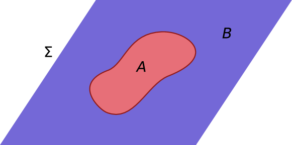
Figure 1: A hypersurface $\Sigma$ divided into two complementary subregions A and B.

Substituting (2) back into (1), we get the entropy associated to region $A$ as

$$S_{A}=-\text{Tr}\rho_{A}\ln\rho_{A}\ ,$$ (3)

which can be designated as the entanglement entropy between regions $A$ and $B$ if the original density matrix $\rho$ was pure. (We would of course get exactly the same answer if we instead traced over the degrees of freedom of $A$ and computed $S_{B}$.)

This definition of entanglement entropy is unsatisfactory for more than one reason. First of all, it does not work for a causal set, because we lack in that setting a notion of data on a hypersurface. Even in the continuum moreover, a hypersurface-based definition of entanglement entropy seems questionable. Essential to getting a finite entanglement entropy is a UV cutoff, and a cutoff referred to a spacelike surface has no reason to be covariant. Two partial Cauchy surfaces sharing the same boundary would then have no reason to carry equal entanglement entropies, even if their domains of dependence were the same. It would thus be difficult to trust results relying on a hypersurface-based cutoff, such as area law scalings. Also in a dynamical spacetime it would be difficult to keep track of the entropy in a consistent way from one time to another using such a cutoff. There is also the problem that strictly speaking (and especially in interacting theories) quantum fields confined to a hypersurface do not make sense, since they only become well defined when smeared in time.

Fortunately there exists a more covariant definition of entanglement entropy which is formally equivalent to (3) in a globally hyperbolic spacetime, but which does not need to appeal to the notion of state on a hypersurface. Moreover, this definition extends naturally to the causal set context, allowing one to take advantange of the Lorentz invariant cutoff which a causal set naturally provides. RDS1 So far, this definition has been developed for the theory of a gaussian scalar field (also called a free scalar field in a quasi-free state). A definition for a fermionic field is soon to appear. We review the definition for the scalar field next.

2 The Entropy of a Gaussian Field

Let us review the definition of entanglement entropy in RDS1 . For a more detailed review, we refer the reader to SSY , and for the full derivation to RDS1 .

The goal is to express $S$ directly in terms of the field correlators. Consider first a single degree of freedom. We introduce the Wightman and Pauli-Jordan matrices,

$$W=\left(\begin{array}[]{cc}\langle qq\rangle&\langle qp\rangle\\ \langle pq\rangle&\langle pp\rangle\\ \end{array}\right)$$ (4)

and

$$i\Delta=\left(\begin{array}[]{cc}0&i\\ -i&0\\ \end{array}\right)\ .$$ (5)

The matrix $W$ corresponds in the field theory to $W(x,x^{\prime})=\langle 0|\phi(x)\phi(x^{\prime})|0\rangle$, while $\Delta$ gives the imaginary part of $W$ and corresponds to the commutator function defined by $i\Delta(x,x^{\prime})=[\phi(x),\phi(x^{\prime})]$. Once we have these, we can express the entropy as a sum over the solutions $\lambda$ of the generalized eigenvalue problem:

$$W\,v=i\lambda\;\Delta\,v\ ,\indent\phantom{where}\indent\Delta\,v\neq 0\ ,$$ (6)

where the arguments of $W$ and $\Delta$ are restricted to the region in question. In a causal set of finite cardinality, or in the continuum with a mode cutoff, (6) becomes a matrix equation where $W$ and $\Delta$ are finite dimensional matrices and $v$ is a finite dimensional vector in the image of $\Delta$. The specific matrices and the corresponding vector solutions $v$ will depend on the nature of the cutoff and on the background spacetime or causal set on which they are defined. The final expression for the entropy of the region is

$$S=\sum\limits_{\lambda}\lambda\,\ln|\lambda|\ .$$ (7)

In certain cases where we restrict $W$ and $\Delta$ to subregions within a larger region or within an entire spacetime or causal set, (7) can be interpreted as an entanglement entropy. In SSY , (7) was applied to some examples in flat two-dimensional spacetimes, and the conventional results for the scaling of the entropy with the UV cutoff were found. In the next section we will apply (7) to the causal set counterparts of the examples treated in SSY . In Section 4, we will apply it to obtain an entropy of coarse-graining for a causal set.

3 Causal Set Entanglement Entropy

Causal set theory CS is an approach to quantum gravity where the deep structure of spacetime is discrete. A causal set is a locally finite partially ordered set. Its elements are the “spacetime atoms”, and its defining order-relation is to be interpreted as the relation of causal or temporal precedence between elements. In the continuum the causal order and the spacetime volume are enough to recover geometry. An important feature of the theory is that in contrast to regular lattices, causal sets are effectively Lorentz invariant. For introductions to causal set theory, we refer the reader to rev1 ; rev2 .

Consider now a free gaussian scalar field living on a causal set which is well approximated by a so-called causal diamond in a 2d Minkowski spacetime. Using the spacetime definition of entropy which was reviewed in the previous section, let us compute the entropy associated to a smaller causal-set causal diamond nested within the larger one. Our setup is shown in Figure 2, and the entropy we will compute can be interpreted as that of the entanglement between the small region and its “causal complement”. In less global terms, it is the entanglement entropy between the “equator” of the smaller region, and its complement within the Cauchy surface produced by extending this equator to the larger region.

In the larger diamond, we use the $W$ of the Sorkin-Johnston vacuum SJ1 ; SJ2 ; Yas , $W_{SJ}$, which is the positive part of the operator $i\Delta$, where

$$\Delta(x,y)=G_{R}(x,y)-G_{R}(y,x),$$ (8)

$G_{R}(x,y)$ being the retarded Green function. For a (free) massless scalar field, $G_{R}$ is simply related to the causal matrix: $G_{R}=\frac{1}{2}C$, where C is the causal matrix,

$$C_{xy}:=\begin{cases}1,&\text{if $x\prec y$}\\ 0,&\text{otherwise}\end{cases}$$ (9)

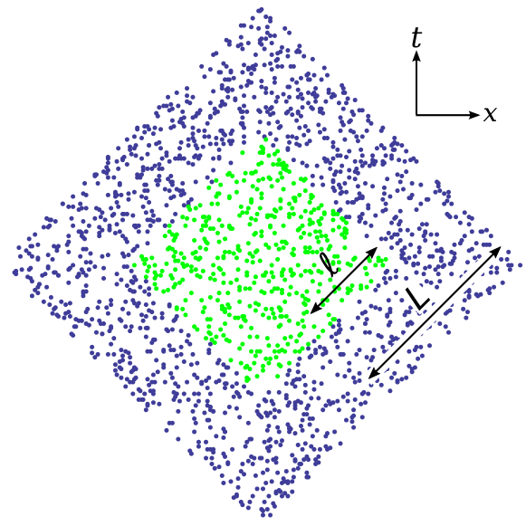
Figure 2: Causal sets of two causal diamonds.

In solving (6), we restrict $W$ and $\Delta$ to elements within the smaller diamond in Figure 2, keeping only the submatrices $W_{xy}$ and $\Delta_{xy}$ such that $x$ and $y$ are in the smaller diamond. In order to assess how the entropy scales with the UV cutoff, we hold the ratio of the sizes of the diamonds fixed and vary the number of elements sprinkled into them. Then the UV cutoff (given by the discreteness length-scale, which is in this case square root of the density of elements) is proportional to $\sqrt{N}$ where $N$ is the number of the causet elements. The UV cutoff is of course proportional to the square root of the number of elements in both the larger and the smaller diamond; we will use the number of elements in the smaller diamond, $N_{\ell}$, to express it.

We find, via numerical simulations, that the entanglement entropy grows linearly with the number of elements in the smaller diamond, thus obeying a spacetime-volume law! The expectation, of course, was that (in $1+1$D) the entropy would scale logarithmically with the UV cutoff (which would mean logarithmic scaling with $\sqrt{N}$ and therefore with $N$ itself), as in the continuum theory SSY ; acr . Furthermore, we find that the entropy in the causet is larger in magnitude (values of order $100$) in comparison with the results in the continuum (order 1 values). Two examples of this linear scaling are shown in Figures 4 and 4, for $\ell/L=1/4$ and $\ell/L=1/2$, respectively. The results fit $S=aN+b$ with $a=0.46$ and $b=-3.20$ for $\ell/L=1/4$, and $a=0.32$ and $b=-6.64$ for $\ell/L=1/2$.

We also find that this spacetime-volume law persists for the massive theory, in $3+1$ dimensions, and when working with nonlocal Green functions such as that obtained from the $G_{R}$ resulting from inverting the d’Alembertian defined in dal . See Appendix C of yasthesis for more details on these cases. This suggests that it is a generic feature of the direct application of (6)-(7) to causal sets.

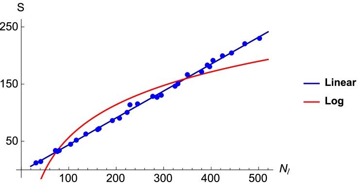
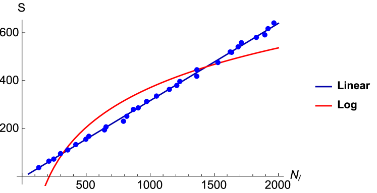
Figure 3: $S$ vs $N_{\ell}$ when $\ell/L=1/4$, along with best fits for linear and logarithmic functions. $N_{\ell}$ is the number of causet elements in the smaller diamond.

Figure 4: $S$ vs $N_{\ell}$ when $\ell/L=1/2$, along with best fits for linear and logarithmic functions. $N_{\ell}$ is the number of causet elements in the smaller diamond.

Whence comes this “extra” entropy? The spectrum of $-i\Delta^{-1}W$ on a causal set necessarily has the same form as in the continuum, in that its eigenvalues come in pairs of $\lambda$ and $1-\lambda$. However, many more of these pairs contribute to the entropy than in the analogous continuum calculation. A closer look at the spectrum of $i\Delta$ reveals how this happens. In the definition (7) it is crucial that we exclude functions in the kernel of $i\Delta$, for which $\lambda$ would not even be defined. (Doing this also ensures that we have enough constraints to enforce the equations of motion, so that only linearly independent degrees of freedom remain.) While excluding the kernel is a simple task for the continuum $i\Delta$, its meaning is not so straightforward for the causal set $i\Delta$. In the continuum, the number of “zero-modes” of $i\Delta$ is huge, but in the causet it is much smaller. Instead of strict zeroes one finds many small but finite eigenvalues that have no counterpart in the spectrum of the continuum $i\Delta$. Even though these eigenvalues are very small, they can contribute a large amount of entropy due to their being so numerous and to the inversion of $\Delta$ in $-i\Delta^{-1}W$.

This observation leads to the idea that (as suggested to us by Siavash Aslanbeigi) these “almost zero-modes” of $i\Delta$ might be the source of the discrepancy between causet and continuum, and that they should be excluded from the entropy calculation if one aims at agreement with the continuum. If we start removing the contributions from the smallest eigenvalues $\tilde{\lambda}$ of $i\Delta$, the scaling of the entropy with the cutoff indeed becomes logarithmic. If the magnitude of the smallest eigenvalue whose contribution we keep is approximately $\tilde{\lambda}_{min}\sim\sqrt{N}/4\pi$, then we get not only the expected scaling-law but also the expected coefficient $1/3$ Cardy .

An example of the logarithmic shape of the data points after the truncation of $i\Delta$ is shown in Figure 5 for $\ell/L=1/2$. In Figure 5, the spectrum of $i\Delta$ has been truncated such that $\tilde{\lambda}_{min}\sim\sqrt{N_{L}}/4\pi$ in the larger diamond and $\tilde{\lambda}_{min}\sim\sqrt{N_{\ell}}/4\pi$ when the restriction is made to the smaller diamond, with contributions from the truncated eigenfunctions being projected out of $W$ as well. (We first truncate both $\Delta$ and $W$ in the larger diamond ($\Delta$ being the antisymmetric part of $W$). We then restrict both matrices to the smaller diamond. Call these restricted matrices $W^{R}$ and $\Delta^{R}$. We then do a second truncation on them, based on the spectrum of $\Delta^{R}$.) A fit to $S=a\ln(x)+b$, with $x$ being $\sqrt{N_{\ell}}/4\pi$ in the smaller diamond, yielded $a=0.346\pm 0.028$ and $b=1.883\pm 0.035$, consistent with the continuum value of $a=1/3$. It is worth emphasizing that the truncation has to be done both in the larger diamond and in the smaller diamond.

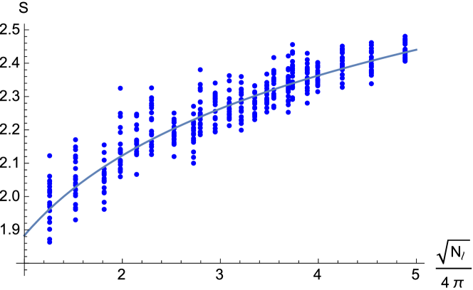
Figure 5: S vs. $\sqrt{N_{\ell}}/4\pi$, after the spectrum of $i\Delta$ has been truncated such that $\tilde{\lambda}_{min}\sim\sqrt{N_{L}}/4\pi$ in the larger diamond and $\tilde{\lambda}_{min}\sim\sqrt{N_{\ell}}/4\pi$ in the smaller diamond.

With hindsight we can understand why the magnitude of the smallest eigenvalue has to be $\sim\sqrt{N}/4\pi$ for consistency with the continuum results. The spectrum of $i\Delta$ in the continuum has dimensions of area, while its spectrum in the causal set is dimensionless. This dimensional observation, together with a comparison of the largest eigenvalues of $i\Delta$ between continuum and causal set, shows that the two spectra can be related by a density factor: $\tilde{\lambda}^{cs}=\rho\tilde{\lambda}^{cont}$, where $\rho=N_{\ell}/4\ell^{2}$. Converting our $\tilde{\lambda}^{cs}_{min}$ to a $\tilde{\lambda}^{cont}_{min}$ (in the small diamond), we find

$$\begin{split}\tilde{\lambda}^{cont}_{min}&=\tilde{\lambda}^{cs}_{min}/\rho\\ &=\sqrt{N_{\ell}}/4\pi\rho\\ &\sim\frac{{\ell}^{2}}{\pi\sqrt{N_{\ell}}},\end{split}$$ (10)

This is precisely the minimum eigenvalue which we retained in the continuum, after imposing our cutoff on the wavelength of the eigenmodes of $i\Delta$. This is reviewed in Appendix A. Eigenvalues smaller than $\tilde{\lambda}^{cs}_{min}$ thus correspond to solutions beyond the cutoff, and are the ones we wish to exclude.

Another way to think of where the $\sqrt{N}/4\pi$ comes from is the following. On one hand, the causet provides a fundamental length given (in 2d) by $\rho^{-1/2}$, and in this sense it serves as a “low pass filter” in relation to the continuum. On the other hand, in the continuum we know exactly the relation between wavelength and eigenvalue for eigenfunctions of $\Delta$ in a causal diamond. If by means of this relation, we convert a cutoff at wavelength $\rho^{-1/2}$ into a cutoff on the spectrum of $\Delta$, we obtain the truncation rule stated above. To the extent, then, that the asymptotic form of the wavelength-eigenvalue relation is universal (as one might expect it to be), one would expect to use a qualitatively similar eigenvalue-cutoff, not just for a causal diamond (order-interval), but for a spacetime region of any shape.

Truncating the spectrum of $i\Delta$ in the causal set by requiring its smallest eigenvalue to be $\tilde{\lambda}_{min}\sim\sqrt{N}/4\pi$ reduces the size of the spectrum from $\sim N$ to $\sim\sqrt{N}$. Thus, a large number of these approximate kernel-modes need to be eliminated if one wishes to recover an area law.

Figure 6 compares the positive spectrum of $i\Delta$ in the causal set with that in the continuum, using a log-log plot. The causal set comprises 200 elements sprinkled with a density of 50. The red dots are the continuum eigenvalues, the blue dots those of the causet appropriately rescaled by a factor of $1/\rho$ for the comparison, and the green dashed line is at $\tilde{\lambda}^{cs}=\sqrt{N}/4\pi$, where we would expect the causet spectrum to end if it were to agree with the continuum. As one sees, the eigenvalues above this line are in good agreement between causet and continuum, but in very poor agreement below it. In particular, there is a “break” in the causet spectrum around where the truncation has to be done. Evidently, this spectral feature could also be used as a guide for where to truncate.

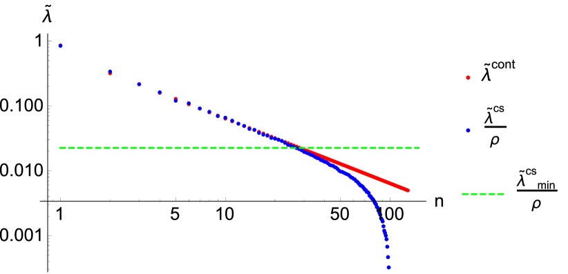
Figure 6: Comparison of the positive spectrum of $i\Delta$ in the continuum and causal set. The causal set has 200 elements and a density of 50. The green dashed line is where $\tilde{\lambda}^{cs}=\sqrt{N}/4\pi$.

In summary, we have seen in these examples, that one can recover continuum-cum-cutoff behaviour from the causal set by modifying the condition $\Delta\,v\neq 0$ in (6) so as to exclude not only the strict zero-modes of $\Delta$, but also its near-zero modes. That is, one identifies those modes $v$ for which $i\Delta\,v=\tilde{\lambda}v$ with $|\tilde{\lambda}|<\sqrt{N}/4\pi$ and projects them out from W and $\Delta$ (doing so in both the bigger and smaller diamonds.)

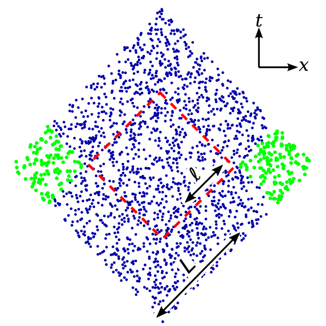
Figure 7: The domain of dependence of the complement of the “Cauchy surface” in the causal diamond.

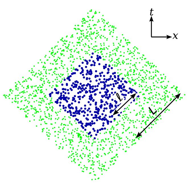
Figure 8: The spacetime volume of the complement of the inner causal diamond.

On the other hand, if one does not project out the near-zero modes, then instead of the area-law familiar from the continuum, one encounters an entropy that scales like spacetime volume. Should this extra entropy be regarded as physical, and if so how should it be interpreted?

In one way the resemblance with entanglement entropy is strong. We began in the larger diamond with a “vacuum” whose entropy vanished, and we found on restricting it to a subregion (the smaller diamond) that it induced there an “impure state” with nonzero entropy. All this resembles the entanglement-entropy associated with a bipartite system in an overall pure state. However the resemblance ends when one asks what could play the role of the “complementary subsystem” to the smaller diamond, in the sense of Figure 1.

Naively one might expect the complement of the inner diamond in Figure 2 to be either the green subset of Figure 7 (the “domain of dependence” of the complement taken within the “Cauchy surface”) or perhaps the green subset in Figure 8 (the spacetime-complement of the smaller diamond itself). But restriction of the scalar field to either of these subregions fails (when one does not truncate the spectrum of $\Delta$) to yield an entropy equal to that within the inner diamond, in conflict with the fact that (bipartite) entanglement entropy can be computed equally well from either one of the two complementary subsystems.

For the region of Figure 8 this shouldn’t be surprising, because the putatively complementary subregions are not mutually spacelike, and the operators therein do not commute with one another. Thus, even in the continuum, one would not expect their entropies to be equal. The situation is otherwise with the green subset of Figure 7. In the continuum, it would be the “causal complement” of the smaller diamond, and the two regions together would have the big diamond as their domain of dependence or “causal development”. The subregional entropies would be equal in that case. That they are unequal here is not an inconsistency because the operators from the two regions taken together don’t necessarily generate the full algebra of operators of the big diamond. In some sense, we are dealing algebraically with a “tripartite” situation, but whether a meaningful entanglement-entropy can be identified in this situation remains unclear. Note however, that if we perform the truncations in the causal set case, then the entropy of the inner diamond indeed becomes equal to that of its causal complement in Figure 7.

A final question arises in connection with the conjecture that black hole entropy is, partly or wholly, entanglement entropy. If this is true then what role if any could an entropic volume-law play in relation to area-law scaling of black hole entropy as usually understood?

4 Entropy of Coarse-Graining

In this section we study the entropy of coarse-graining by decimation and blocking. We study decimation in both causal sets and a chain of harmonic oscillators, and blocking in a chain of harmonic oscillators. There is no known way to coarse-grain by blocking in a causal set. We use (7) for the causal set calculation, and the formalism of RDS2 for the oscillator calculations.

The Lagrangian for the chain of oscillators we consider is

$$\mathcal{L}=\frac{1}{2}\left(\sum_{N=1}^{N_{max}}\hat{\dot{q}}_{N}^{2}-\sum_{N,M=1}^{N_{max}}V_{MN}\,\hat{q}_{N}\,\hat{q}_{M}\right)=\frac{1}{2}\sum_{N=1}^{N_{max}}[\hat{\dot{q}}_{N}^{2}-m^{2}\hat{q}_{N}^{2}-k(\hat{q}_{N+1}-\hat{q}_{N})^{2}],$$ (11)

where k is the coupling strength between the oscillators, and in terms of the spatial UV cutoff $a$, $k=1/a^{2}$ gold . We set $k=10^{6}$. We consider the massless theory with periodic boundary conditions and mass regulator $m^{2}=10^{-6}$.

In coarse-graining by decimation, we iteratively remove $10\%$ of the causet elements and oscillators. In the causet we remove each element with probability $0.1$, and in the chain of oscillators we remove each oscillator with probability $0.1$. In more detail, at first we divide the oscillators and causal set elements into two subsets: one subset containing (approximately) $90\%$ of the oscillators and causet elements, and the other (complementary) subset containing the remaining (approximately) $10\%$. This division is done randomly, so the oscillators in one subset may not necessarily have all of their nearest neighbours from the full chain in that subset. Similarly, the elements of the subset of the causal set are randomly chosen. Then we compute the entanglement entropy between the two subsets. This is our first (non-zero) entropy data point. Subsequently, we divide the subset containing $\sim 90\%$ of the original oscillators and causet elements into two subsets containing $\sim 90\%$ and $\sim 10\%$ of them. We then group this second $\sim 10\%$ subset with the first $\sim 10\%$ subset, such that in terms of the original number of oscillators, our two subsets at this second iteration contain $\sim 81\%$ and $\sim 19\%$ of the total number of original oscillators and elements. The entanglement entropy between these two subsets gives us our second (non-zero) entropy data point. Similarly, each $n^{th}$ time we carry this out, we will have $\sim 0.9^{n}$ and $\sim 1-0.9^{n}$ of the original number of oscillators and causet elements in the two subsets whose entanglement entropy we compute.

A simple relation is obtained in both cases. The entropy depends quadratically on the number of degrees of freedom (DoF’s) remaining after coarse-graining. Initially, when all DoF’s are present, the entropy is 0. It rises and reaches a maximum when about half of the DoF’s remain, after which it drops, symmetrically, until it reaches 0 again when there are no more DoF’s left.

The causal set result without truncating $i\Delta$ and $W$ is shown in Figure 9, where the entropy is plotted versus the number of elements remaining in the causal diamond. Initially the diamond contained 4048 sprinkled elements and had a density of $10.12$. The results fit $S=aN^{2}+bN+c$ with $a=-1.5\times 10^{-4},\,b=0.60,\,\text{and}\,c=7.0$.

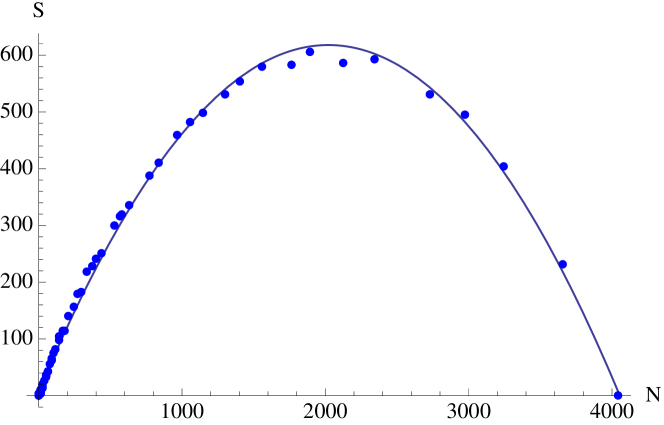
Figure 9: $S$ vs. $N$ in a causet under coarse-graining (without truncating $i\Delta$ and $W$) by decimation: we remove elements with probability 0.1.

The causal set result with truncated $i\Delta$ and $W$ is shown in Figure 10, where the entropy is plotted versus the square root of the number of elements remaining in the causal diamond. Initially the diamond contained 4048 sprinkled elements. The results fit $S=aN+b\sqrt{N}+c$ with $a=-0.0019,\,b=0.12,\,\text{and}\,c=-0.40$.

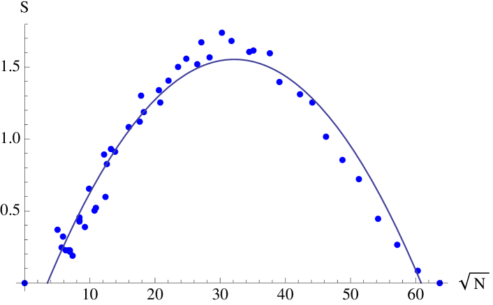
Figure 10: $S$ vs. $\sqrt{N}$ in a causet under coarse-graining (with truncated $i\Delta$ and $W$) by decimation: we remove elements with probability 0.1.

It should be noted that the DoF’s in terms of which we get a parabolic relation for the entropy of coarse-graining are different for the truncated and full $i\Delta$ and $W$. For the full $i\Delta$ and $W$ the DoF’s are counted by the number of elements remaining in the diamond, $N$, and for the truncated $i\Delta$ and $W$ they are counted by $\sqrt{N}$.

The result for the chain of oscillators is shown in Figure 11, where the entropy is plotted versus the number of oscillators remaining in the chain. Initially the chain contained 1000 oscillators. The results fit $S=aN^{2}+bN+c$ with $a=-5.1\times 10^{-4},\,b=0.51,\,\text{and}\,c=5.4$.

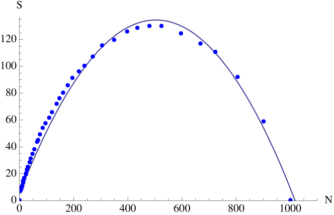
Figure 11: $S$ vs. $N$ in a chain of oscillators under coarse-graining by decimation: we remove elements with probability 0.1.

In coarse-graining by blocking, we rewrite the $q_{i}$’s in terms of $Q_{i}^{\pm}$’s defined as $Q_{1}^{\pm}\equiv(q_{1}\pm q_{2})/2$, $Q_{2}^{\pm}\equiv(q_{3}\pm q_{4})/2$, … We then discard all $Q^{-}$’s, thus reducing the DoF’s by half. In the next iteration we work in terms of $(Q^{+}_{1}\pm Q^{+}_{2})/2$, $(Q^{+}_{3}\pm Q^{+}_{4})/2$… and repeat. The result for the entropy of coarse-graining by blocking in a chain of oscillators is shown in Figure 12. The entropy is shown versus the number of oscillators remaining in the chain. Initially the chain contained $2^{14}$ oscillators. The results fit $S=aN^{2}+bN+c$ with $a=-9.4\times 10^{-6},\,b=0.15,\,\text{and}\,c=-0.36$.

Thus entropy of coarse-graining by both decimation and blocking have led to a parabolic dependence on the number of remaining DoF’s, in our examples. Our results suggest that this entropy of coarse-graining might have universal properties that would be interesting to investigate further. We frequently deal with coarse-grained versions of certain systems, and there seems to be an entropy associated to this coarse-graining which has universal properties that would be useful to understand.

Our choices of parameters ($\rho$ for the causal set, and $m$ and $k$ for the oscillators) in this section were arbitrary. As we change the values of these parameters (as long as the UV cutoffs $\rho$ and $k$ remain large such that the asymptotic form of the entropy holds, and as long as the mass, $m$, remains finite in order to avoid the infrared divergence discussed in YKY ), the qualitative results of this section do not change (as unpublished investigations have shown). The magnitude of the maximum of the quadratic relation (Figures 9–12) will, however, depend on these parameters. It would be interesting to analyze how this maximum scales with each of the parameters. We defer this study to future work.

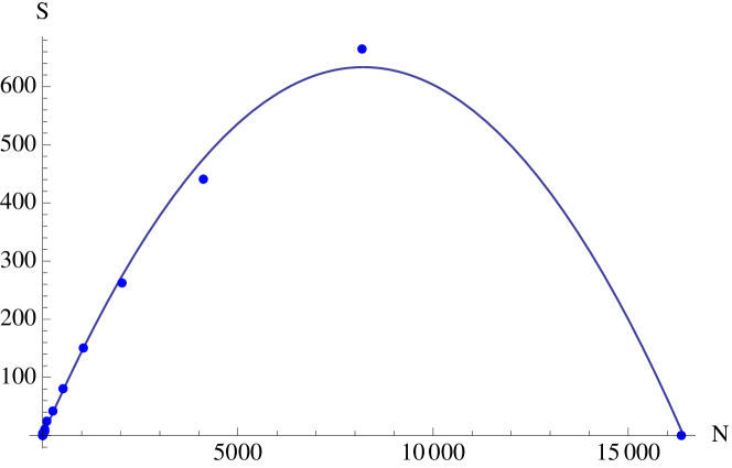
Figure 12: $S$ vs. $N$ in a chain of oscillators under coarse-graining by blocking.

5 Conclusions

In the present paper, we have studied (primarily by computer simulations) the entanglement entropy of a free scalar field in causal sets well approximated by regions of $1+1$D flat spacetime. Initially we found unexpectedly that instead of the conventional spatial area law (logarithmic scaling of entropy with UV cutoff), a spacetime-volume scaling was obtained. We attributed this difference between the causet and the continuum, to a difference in the near-zero part of the spectrum of $i\Delta$. With this in mind, we identified, in the causet case, a minimum eigenvalue of $i\Delta$ which answers to the fundamental discreteness scale embodied in the causet itself. And we found that when the spectrum of $i\Delta$ was truncated there (and the contributions of these parts removed from $W$ as well), the continuum area law was recovered.

With these findings, we are beginning to understand entanglement entropy in causal set theory. This is important for causal sets, of course, but it also demonstrates an important point of principle, namely that the UV cutoff needed to render entanglement entropy finite can be introduced without doing violence to Lorentz symmetry. The way now seems open to begin to address questions which hinge on understanding the entropy of entanglement associated with black hole horizons, ultimately the question whether most or all of the horizon entropy can be traced to entanglement of one sort or another.

Work is also underway to find the entropy associated to the event horizon of an “observer” in de Sitter spacetime yasds . The retarded Green function in a $3+1$D de Sitter causal set has recently been found sumatidS and makes possible the entropy calculation in that setting. Also soon to appear is an application of the truncation scheme presented in this paper to the Pauli-Jordan function derived from the retarded Green functions which are inverses of the nonlocal causal set d’Alembertians dionentropy .

It is not yet known how the truncation procedure described in this paper will generalize to higher dimensions, and for arbitrary spacetime regions. One speculation is that in $d$ spacetime dimensions, the magnitude of the smallest eigenvalue is always of the order of $N^{1/d}$. Another simple possibility for the generalization of the truncation scheme is to include the largest $N^{(d-1)/d}$ eigenvalues (possibly with a pre-factor that could depend on the shape of the region) in $d$ spacetime dimensions. Both of these possibilities are currently under investigation. Ultimately, however, to successfully generalize this truncation scheme we would need to gain a better understanding of the asymptotic (in the UV regime) nature of the eigenfunctions and spectrum of $i\Delta$ in a general setting. Some ideas in this direction (involving a conjecture that these eigenvalues resemble a class of wavepackets and/or wavelets) are being pursued.

Whether the entropy-formula we have used will generalize to interacting or non-gaussian theories, and if so how, is also an open question. Any such formula would necessarily have to supplement information from the Wightman or “two-point” function with information corresponding to correlators of higher degree. Conversely the full complement of $n$-point functions should determine the entropy uniquely, at least in principle. Perhaps a perturbative expansion about the gaussian case could be formulated for interacting theories. Or perhaps if the entropy-definition in the gaussian case could be recast in path-integral form (for example, if it could be expressed as a sum over the eigenvalues of a decoherence functional or other quantity related to the path integral), the resulting expression could be generalized to the non-gaussian case.

The methods we have used in our simulations could also prove valuable in a continuum context, as they illustrate how simulating entanglement entropy via sprinkled causal sets can expedite calculations which would otherwise be more tedious.

6 Acknowledgements

We thank Niayesh Afshordi, Achim Kempf, Sumati Surya, Mehdi Saravani, and Fay Dowker for helpful discussions. This research was supported in part by NSERC through grant RGPIN-418709-2012. This research was supported in part by Perimeter Institute for Theoretical Physics. Research at Perimeter Institute is supported by the Government of Canada through the Department of Innovation, Science and Economic Development Canada and by the Province of Ontario through the Ministry of Research, Innovation and Science.

Appendix A Entanglement Entropy in Continuum Diamonds

A.1 Entanglement Entropy

In this Appendix, we review the main results of SSY .

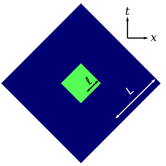
Figure 13: Two nested causal diamonds.

We wish to use (7) to compute the entanglement entropy of a scalar field, resulting from restricting it to a smaller causal diamond within a larger one in $1+1$D Minkowski spacetime. The setup is the continuum analogue of Figure 2, shown in Figure 13. In Minkowski lightcone coordinates $u=\frac{t+x}{\sqrt{2}}$ and $v=\frac{t-x}{\sqrt{2}}$,

$$\Delta(u,v;u^{\prime},v^{\prime})=\frac{-1}{2}[\theta(u-u^{\prime})+\theta(v-v^{\prime})-1],\$$ (12)

and

$$W=-\frac{1}{4\pi}\mathrm{ln}|\Delta u\Delta v|-\frac{i}{4}\text{sgn}(\Delta u+\Delta v)\theta(\Delta u\Delta v)-\frac{1}{2\pi}\mathrm{ln}\frac{\pi}{4{L}}+\epsilon+\mathcal{O}\left(\frac{\delta}{{L}}\right),$$ (13)

where $\epsilon\approx-0.063$ when $\ell\ll L$, and $\delta$ collectively denotes the coordinate differences $u-u^{\prime},v-v^{\prime},u-v^{\prime},v-u^{\prime}$. We set $\frac{{\ell}}{L}=.01$.

We understand the properties of $\Delta$ and $W$ in this spacetime Yas .

We represent $W$ and $\Delta$ as matrices in the eigenbasis of $i\Delta$ which consists of two sets of eigenfunctions:

$$f_{k}(u,v) :=e^{-iku}-e^{-ikv}, \textrm{with }k=\frac{n\pi}{{\ell}},\;n=\pm 1,\pm 2,\ldots$$

$$g_{k}(u,v) :=e^{-iku}+e^{-ikv}-2\cos(k{\ell}), \textrm{with }k\in\mathcal{K},$$ (14)

where $\mathcal{K}=\left\{k\in\mathbb{R}\,|\,\tan(k{\ell})=2k{\ell}\ \textrm{and}\ k\neq 0\right\}$.

The eigenvalues are ${\lambda}_{k}={\ell}/k$, and the $L^{2}$-norms are $||{f}_{\small{k}}||^{2}=8{{\ell}}^{2}$ and $||{g}_{\small{k}}||^{2}=8{{\ell}}^{2}-16{{\ell}}^{2}{\cos}^{2}(k{\ell})$.

For the representation of $W$, we computed $\langle f_{k}|W|f_{k^{\prime}}\rangle$ and $\langle g_{k}|W|g_{k^{\prime}}\rangle$. The terms $\langle f_{k}|W|g_{k^{\prime}}\rangle$ vanish, making $W$ block diagonal in this basis.

The matrices representing $W$ and $\Delta$ are truncated to retain only a finite number of eigenfunctions $f_{k}$ and $g_{k}$ up to a maximum value $k=k_{max}=n_{max}\pi/\ell$. Initial conditions described by functions with wavelengths greater than $\lambda_{min}\sim 1/k_{max}$, can be expanded in terms of these modes. A natural choice for the cutoff is therefore $1/k_{max}$. In the calculations, we keep $\ell/L$ fixed and vary $k_{max}$ (or equivalently $n_{max}$). The eigenvalues are all of order one with absolute value less than 3. All but a handful of the eigenvalue-pairs have values close to $1$ and $0$.

The obtained values of $S$, shown in Figure 14, are fit almost perfectly by the curve

$$S=b\ln\left[\frac{{\ell}}{a}\right]+c_{1}$$ (15)

with $b=0.33277$ and $c_{1}=0.70782$.

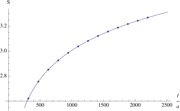
Figure 14: Data points represent calculated values of $S=\sum\lambda\,\ln|\lambda|$ in the continuum causal diamonds of Figure 13.

A.2 Rényi Entropies

We can extend the results of SSY to include Rényi entropies. The spacetime definition of entropy given in RDS1 can be generalized for Rényi entropies of order $n$, $S^{(n)}$, in the following way:

$$S^{(n)}=\sum_{\lambda}\frac{-1}{1-n}\ln(\lambda^{n}-(\lambda-1)^{n})\ ,$$ (16)

where $\lambda$ and $1-\lambda$ are solutions to the generalized eigenvalue problem (6). The spacetime we apply this formula to is again Figure 13. The expected result Cardy is that the entropies should scale as:

$$S^{(n)}=\frac{1}{6}(1+\frac{1}{n})\ln(\frac{\ell}{a})+c_{n}$$ (17)

where $c_{n}$ are non-universal constants.

Figures 15-16 show the results from (16) for $S^{(2)}$ and $S^{(3)}$. There is good agreement between them and (17), with more deviation present for the higher order Rényi entropies. The scaling coefficients found from (16) for $S^{(2)}$ to $S^{(10)}$ are:

$$\{0.24961,0.221498,0.206892,0.197726,0.191411,0.18682,0.183354,0.18066,0.178517\},$$ (18)

to be compared with those from (17):

$$\{0.25,0.222222,0.208333,0.2,0.194444,0.190476,0.1875,0.185185,0.183333\}.$$ (19)

Figure 15: 2nd order Rényi entropy $S^{(2)}$ from (16) vs. $\ell/a$ along with a fit to $S=b\ln\left[\frac{{\ell}}{a}\right]+c$.

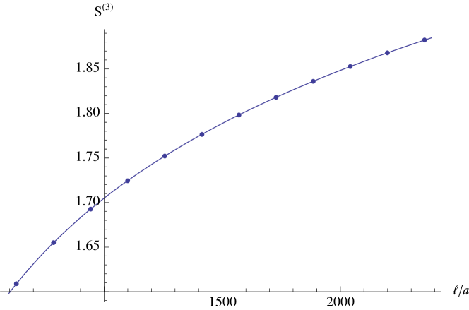
Figure 16: 3rd order Rényi entropy $S^{(3)}$ from (16) vs. $\ell/a$ along with a fit to $S=b\ln\left[\frac{{\ell}}{a}\right]+c$.

References

- (1) R. D. Sorkin, Expressing Entropy Globally in Terms of (4D) Field-Correlations, arXiv:1205.2953 (2012); J. Phys. Conf. Ser. 484 012004 2014; http://www.pitp.ca/personal/rsorkin/some.papers/143.s.from.w.pdf.
- (2) R. D. Sorkin, On the Entropy of the Vacuum Outside a Horizon, in Tenth International Conference on General Relativity and Gravitation (held Padova, 4-9 July, 1983), Contributed Papers, vol. 2, pp. 734736. (1983) arXiv:1402.3589 [gr-qc].
- (3) M. Van Raamsdonk, Building up Spacetime with Quantum Entanglement, Int.J.Mod.Phys.D19:2429-2435, (2010).
- (4) M. Saravani, R. D. Sorkin, and Y. K. Yazdi, Spacetime Entanglement Entropy in 1+1 Dimensions, Class. Quantum Grav. 31 (2014) 214006, arXiv:1311.7146.
- (5) L. Bombelli, J.-H. Lee, D. Meyer, and R. D. Sorkin, Space-Time as a Causal Set, Phys. Rev. Lett. 59, 521 (1987).
- (6) R. D. Sorkin, Causal sets: Discrete Gravity, in A. Gomberoff and D. Marolf (eds), Proceedings of the Valdivia Summer School. arXiv:gr-qc/0309009, (2002).
- (7) J. Henson, The Causal Set Approach to Quantum Gravity, arXiv:gr-qc/0601121, (2006).
- (8) R. D. Sorkin, Scalar Field Theory on a Causal Set in Histories Form, J.Phys.Conf.Ser.306 (2011) 012017, [arXiv:1107.0698].
- (9) S. P. Johnston, Quantum Fields on Causal Sets, PhD thesis, Imperial College, (2010). arXiv:1010.5514.
- (10) N. Afshordi, M. Buck, F. Dowker, D. Rideout, R. D. Sorkin, and Y. K. Yazdi, A Ground State for the Causal Diamond in 2 Dimensions, JHEP 10, 088 (2012), no. 10, arXiv:1207.7101.
- (11) Anushya Chandran, Chris Laumann, and Rafael D. Sorkin, When is an area law not an area law? Entropy 18 240 2016, http://arxiv.org/abs/1511.02996; http://www.pitp.ca/personal/rsorkin/some.papers/151.area.law.pdf
- (12) R. D. Sorkin, Does Locality Fail at Intermediate Length-Scales, in Approaches to Quantum Gravity; Towards a New Understanding of Space and Time, edited by Daniele Oriti, Cambridge University Press (2009) 26 43, [gr-qc/0703099].
- (13) Y. K. Yazdi, Entanglement Entropy of Scalar Fields in Causal Set Theory, PhD thesis, UWSpace (2017), http://hdl.handle.net/10012/12151.
- (14) P. Calabrese and J. Cardy, Entanglement Entropy and Conformal Field Theory, J. Phys. A 42, 504005 (2009), arXiv:0905.4013.
- (15) Luca Bombelli, Rabinder K. Koul, Joohan Lee and Rafael D. Sorkin, A Quantum Source of Entropy for Black Holes, Phys. Rev. D34, 373-383 (1986).
- (16) H. Goldstein, Classical Mechanics, Addison-Wesley, (1950).
- (17) Y. K. Yazdi, Zero Modes and Entanglement Entropy, JHEP 04 (2017) 140, arXiv:1608.04744.
- (18) S. N. Ahmed, S. Surya, and Y. K. Yazdi (in preparation).
- (19) S. N. Ahmed, F. Dowker, and S. Surya, Scalar Field Green Functions on Causal Sets, (2017), Class. Quantum Grav. 34 124002, arXiv:1701.07212.
- (20) D. Benincasa, A. Belenchia, M. Letizia, and S. Liberati (in preparation).