Unconventional fermionic pairing states in a monochromatically tilted optical lattice

Abstract

We study the one-dimensional attractive Fermionic Hubbard model under the influence of periodic driving with the time-dependent density matrix renormalization group method. We show that the system can be driven into an unconventional pairing state characterized by a condensate made of Cooper-pairs with a finite center-of-mass momentum similar to a Fulde-Ferrell state. We obtain results both in the laboratory and the rotating reference frames demonstrating that the momentum of the condensate can be finely tuned by changing the ratio between the amplitude and the frequency of the driving. In particular, by quenching this ratio to the value corresponding to suppression of the tunnelling and the Coulomb interaction strength to zero, we are able to “freeze” the condensate. We finally study the effects of different initial conditions, and compare our numerical results to those obtained from a time-independent Floquet theory in the large frequency regime. Our work offers the possibility of engineering and controlling unconventional pairing states in fermionic condensates.

I Introduction

Cold atoms in optical latticesBloch et al. (2008); Lewenstein et al. (2012) currently represent one of the best candidates for the quantum simulation Buluta and Nori (2009); Bloch et al. (2012); Georgescu et al. (2014) of bosonic and fermionic systems, given the extreme level of tunability of the microscopic Hamiltonian parameters, such as tunneling and interactions. Recent experimental advances allow for site-resolved detection measurementsBakr et al. (2010); Sherson et al. (2010), the simulation of artificial gauge fieldsJaksch and Zoller (2003); Lin et al. (2009); Dalibard et al. (2011); Struck et al. (2012), and also the possibility to control the behavior of the optical lattice under the influence of high frequency electromagnetic fieldsLignier et al. (2007); Zenesini et al. (2009). In addition, intriguing phenomena such as Bloch oscillations and the formation of repulsively bound pairs have been observedWinkler et al. (2006). A particularly interesting phenomenon is provided by the coherent destruction of tunneling, in which driving the system with an oscillating field has the effect of renormalizing the intersite tunneling amplitude. By tuning the amplitude of the driving field, it has been theoretically and experimentally demonstrated that one can induce the superfluid-Mott insulator transitionEckardt et al. (2005).

Theoretically, it has been shown that new exotic interactions and correlated hopping termsDi Liberto et al. (2011) can be effectively generated by the external electromagnetic fields. These achievements have opened a new line of research, termed Floquet engineering. Indeed, both bosonic and fermionic Hubbard models are currently theoretically and experimentally investigated, with the possibility of exploring new exciting physics out of equilibrium.

In Refs. [Creffield and Sols, 2008, 2011], it has been demonstrated that a high-frequency monochomatic external field can be used not only to control the hopping amplitude of cold atoms trapped in a lattice, but also the phase of their wave function. In a one dimensional optical lattice of bosonic atoms described by a Bosonic Hubbard model, the authors showed that a coherent matter current can be generated. The current is induced by a shift in the momentum distribution function’s central peak, which is proportional to the amplitude of the driving force.

In this paper, we apply the same periodic perturbation to a fermionic optical lattice described by the Fermi-Hubbard model. We explore the particular regime of parameters where there is an attractive interaction between the fermionic particles and explore the possibility of realizing and manipulating exotic pairing phases. In this context, Fulde-Ferrell (FF) and Larkin-Ovchinnikov (LO) phases recently attracted a great deal of interest from both the experimentalZwierlein et al. (2006); Partridge et al. (2006); Liao et al. (2010) and the theoretical communityOrso (2007); Feiguin and Heidrich-Meisner (2007); Casula et al. (2008); Lüscher et al. (2008); Rizzi et al. (2008); Tezuka and Ueda (2008); Feiguin et al. (2012); Guan et al. (2013). In the original idea of Fulde and Ferrell, Cooper pairs form with finite center-of-mass momentumFulde and Ferrell (1964). Larkin and Ovchinnikov formulated a related proposal in which the superconducting order parameter oscillates in spaceLarkin and Ovchinnikov (1964). These ideas are closely related, because the inohomogeneus order parameterYang (2001); Casalbuoni and Nardulli (2004) may be interpreted as an interference pattern between condensates with opposite center-of-mass momenta. In our case, we find a pairing state similar to a FF state, consisting of a condensate which moves as a coherent matter field of Cooper-like pairs. In particular, we find that the center-of-mass momentum of the condensate can be tuned by changing the amplitude and the frequency of the external drive.

Using the Floquet formalismBukov and Polkovnikov (2014a, b); Eckardt and Anisimovas (2015); Bukov et al. (2015); Mikami et al. (2016), we also derive an effective time-independent Hamiltonian for the system in the presence of a high-frequency driving force, and compare the results coming from this effective theory by solving the model numerically using the time dependent Density Matrix Renormalization Group method (tDMRG) White and Feiguin (2004a); Daley et al. (2004).

We finally investigate the pairing properties of the system by using different quenching protocols. We propose to abruptly change either the interaction between the fermions, or the parameters of the external driving potential independently. These protocols are investigated numerically using tDMRG and could be experimentally accessible in current experimental setups.

The paper is organized as follows. In Section II we present the model in different reference frames and apply Floquet theory in the rotating frame. In Section III we show that the numerical results obtained with tDMRG are in agreement with Floquet theory. In Section IV we explore different quenching protocols for the characterization of the exotic pairing phase found, and we finally summarize our results in the conclusions.

II MODEL

In this work, we consider a one dimensional Fermionic Hubbard chain subjected to an external time dependent perturbation. The Hamiltonian in the laboratory reference frame is given by $H_{lab}(t)=H+V(t)$, where $H$ is given by the one dimensional Fermi-Hubbard model

$$H=-J\sum\limits_{\langle i,j\rangle,\sigma}(c^{\dagger}_{i,\sigma}c_{j,\sigma}+h.c.)+U\sum\limits_{i}n_{i,\uparrow}n_{i,\downarrow},$$ (1)

while the tilting perturbation is given by

$$V(t)=\theta(t)A\sin(\omega t+\theta)\sum\limits_{i,\sigma}in_{i,\sigma},$$ (2)

and constitutes a linear potential ramp applied to the sites of the lattice suddenly turned on at time $t=0$. Notice that this driving protocol is different from the one adopted in Ref. [Creffield and Sols, 2008], where the amplitude was linearly ramped on in time. In this paper, we assume that the tilting perturbation is sinusoidal, with phase $\theta=0$, amplitude $A$ and frequency $\omega$. In this case, as was observed in Ref. [Creffield and Sols, 2008] and as will be clear below, the effects of the phase of the drive are maximum, giving a non trivial contribution in the effective Floquet description. In the Eq. (1), $J$ is the hopping amplitude between nearest neighbor sites (indicated by $\langle i,j\rangle$), $U$ parametrizes the repulsion between atoms, and $c^{\dagger}_{i,\sigma}$ ($c_{i,\sigma}$) is the standard fermionic creation (annihilation) operator on site $i$ with spin ${\sigma}$ ($\bar{\sigma}$ indicates the opposite of $\sigma$), while $n_{i,\sigma}=c^{\dagger}_{i,\sigma}c_{i,\sigma}$ is the fermionic occupation operator. The Planck constant is set to $\hbar=1$, the lattice parameter $a=1$, and all of the energies are in the units of the hopping $J$. These definitions automatically set the time unit to $\hbar/J$. Throughout this paper we consider an attractive interaction between the fermions $U<0$, a lattice with open boundary conditions and filling $N/L=2/3$, where $N$ is the total number of fermions and $L$ is the system size. It is well known that the low energy physics of the model (1) can be described in terms of a gapped spin mode and a gapless charge mode. The system belongs to the Luther-Emery universality class and superconducting pair correlations are dominant,

$$P_{i,j}=\langle\Delta_{i}^{{\dagger}}\Delta_{j}\rangle\propto|i-j|^{-1/K_{\rho}}$$ (3)

with an non-universal power law decay with exponent $K_{\rho}$ determined by the interaction $U$. The main purpose of this paper is to investigate the properties of the pairing correlation function in Eq. (3) in the presence of the driving (2).

II.1 Laboratory, rotating reference frames, and Floquet approximation

It is useful to remind how an observable quantity is calculated in the laboratory reference frame. At time $t=0$, the ground state $|\Psi_{0}\rangle$ of $H$ is initially calculated. Afterward, the time evolved state $|\Psi_{lab}(t)\rangle=U_{lab}(t,0)|\Psi_{0}\rangle$, where $U_{lab}(t,0)=\mathcal{T}\Big{[}\textrm{exp}(-i\int_{0}^{t}H_{lab}(t^{\prime})dt^{\prime})\Big{]}$, is computed under the action of the entire time dependent Hamiltonian $H_{lab}(t)$, $\mathcal{T}$ being the time-ordering operator. Assuming that the ground state is normalized, an observable $O$ is then calculated computing the expectation value

$$\langle O\rangle_{lab}=\langle\Psi_{lab}(t)|O|\Psi_{lab}(t)\rangle.$$ (4)

We now consider the formulation of the problem in the “rotating” reference frame. We apply to the Hamitonian $H_{lab}(t)$ the following time dependent canonical transformation

$$R(t)=e^{-if(t)\sum_{j}j{\hat{n}}_{j}},$$ (5)

where

$$f(t)=A\int_{0}^{t}d\tau\,\text{sin}(\omega\tau)=A{1-\cos(\omega t)\over\omega}.$$

In this way, the rotated Hamiltonian $H_{rot}(t)=R^{{\dagger}}(t)H_{lab}(t)R(t)-iR^{{\dagger}}(t)\partial_{t}R(t)$ is still time dependent and assumes the form

$$H_{rot}(t) =-J\sum\limits_{\langle i,j\rangle,\sigma}(e^{-if(t)}c^{\dagger}_{i,\sigma}c_{j,\sigma}+h.c.)$$

$$+U\sum\limits_{i}n_{i,\uparrow}n_{i,\downarrow},$$ (6)

where the hopping term acquires a complex nontrivial phase, which is the central quantity in this paper. It is clear that, at $t=0$, $H_{lab}(0)=H_{rot}(0)$. Therefore, once the ground state $|\Psi_{0}\rangle$ is computed, the time evolved state in the rotating frame, $|\Psi_{rot}(t)\rangle$, which can be obtained at each time $t$ from the laboratory frame state vector with $|\Psi_{rot}(t)\rangle=R(t)|\Psi_{lab}(t)\rangle$ reads $|\Psi_{rot}(t)\rangle=U_{rot}(t,0)|\Psi_{0}\rangle$, where $U_{rot}(t,0)=\mathcal{T}\Big{[}\textrm{exp}(-i\int_{0}^{t}H_{rot}(t^{\prime})dt^{\prime})\Big{]}$. An observable can be obtained by evaluating the following expression

$$\langle O\rangle_{rot}=\langle\Psi_{rot}(t)|R(t)OR^{{\dagger}}(t)|\Psi_{rot}(t)\rangle,$$ (7)

where the observable operator should be correctly transformed to the rotated frame. We now apply Floquet theory to the rotated Hamiltonian Eq. (II.1). According to Floquet theorem, the time evolution operator $U(t_{1},t_{2})=\mathcal{T}\Big{[}\textrm{exp}(-i\int_{t_{1}}^{t_{2}}H(t)dt)\Big{]}$ of any time-periodic Hamiltonian $H(t)=H(t+T)$ can be written in the form

$$U(t_{1},t_{2})=\textrm{exp}[-iK_{F}(t_{2})]\textrm{exp}[-iH_{F}(t_{2}-t_{1})]\textrm{exp}[iK_{F}(t_{1})],$$ (8)

where $H_{F}$ is an effective time independent Hamiltonian describing the long time dynamics of the system, called the Floquet Hamiltonian, while $K_{F}(t)=K_{F}(t+T)$ is a time-periodic operator (called kick operator) describing the fast evolution in one period of time $T=2\pi/\omega$. It is well known that in the limit of very large frequency or small period one can calculate the Floquet Hamiltonian and the kick operator perturbatively using a high frequency expansion. In this paper, we use a particular van Vleck expansion, which is invariant under the choice of the driving phase in the rotating frame  Bukov and Polkovnikov (2014a); Eckardt and Anisimovas (2015); Mikami et al. (2016):

$$H_{F}^{(0)} = H_{0}=\frac{1}{T}\int_{0}^{T}H(t)dt$$ (9)

$$H_{F}^{(1)} = \frac{1}{\omega}\sum_{m=1}^{\infty}\frac{1}{m}[H_{m},H_{-m}]=$$

$$= \frac{1}{2!Ti}\int_{0}^{T}dt_{1}\int_{0}^{t_{1}}dt_{2}f(t_{1}-t_{2})[H(t_{1}),H(t_{2})]$$

$$K_{F}^{(0)}(t) = 0$$ (11)

$$K_{F}^{(1)}(t) = \frac{1}{i\omega}\sum_{m\neq 0}\frac{e^{im\omega t}}{m}H_{m}$$ (12)

$$= -\frac{1}{2}\int_{t}^{t+T}dt^{\prime}g(t-t^{\prime})H(t^{\prime}),$$

where we decomposed the Hamiltonian in a Fourier series $H(t)=\sum_{m=-\infty}^{\infty}H_{m}e^{im\omega t}$, with $H_{m}$ operator-valued coefficients; the functions $f$ and $g$ are defined as $f(x)\equiv(1-2x/T)$ and $g(x)\equiv(1+2x/T)$. Recently, the importance of the kick operators in the stroboscopic and non-stroboscopic dynamics of Floquet systems has been highlighted by several authorsBukov and Polkovnikov (2014a, b); Eckardt and Anisimovas (2015); Bukov et al. (2015). For the rotated Hamiltonian in Eq. (II.1), the zero-order Floquet Hamiltonian is given by

$$H_{F}^{(0)} =-JJ_{0}(A/\omega)\sum\limits_{\langle i,j\rangle,\sigma}\Big{(}e^{-i\frac{A}{\omega}}c^{\dagger}_{i,\sigma}c_{j,\sigma}+h.c.\Big{)}$$ (13)

$$+U\sum\limits_{i}n_{i,\uparrow}n_{i,\downarrow},$$

where the amplitude of the hopping matrix element is renormalized by the Bessel function $J_{0}(A/\omega)$. Notice that the hopping in the Floquet Hamiltonian is complex acquiring a phase $\phi=-A/\omega$. This phase comes from transformation to the rotating frame and would be absent for the cosinusoidal driving field Creffield and Sols (2008), which is equivalent to the shift in the rotating frame. The above equation has been derived using the Jacobi-Anger expansion

$$\textrm{exp}\Bigg{[}i\frac{A}{\omega}\cos(\omega t)\Bigg{]}=\sum_{m=-\infty}^{\infty}i^{m}J_{m}(A/\omega)e^{im\omega t},$$ (14)

which allows one to simply calculate the $m$-th component of the Fourier series operator-valued coefficients of the Hamiltonian

$$H_{m} =-JJ_{m}(A/\omega)\sum\limits_{\langle i,j\rangle,\sigma}\Big{(}e^{-i\frac{A}{\omega}}i^{m}c^{\dagger}_{i,\sigma}c_{j,\sigma}+h.c.\Big{)}$$

$$+\delta_{m,0}U\sum\limits_{i}n_{i,\uparrow}n_{i,\downarrow},$$ (15)

where it is important to point out that the interaction part contributes only for $m=0$. Since at zero order of the high frequency expansion the kick operator is zero, the evolution operator in the rotating frame $U_{rot}(t,0)$ becomes simply

$$U_{rot}^{(0)}(t,0)=\textrm{exp}(-iH_{F}^{(0)}t).$$ (16)

Using the Fourier decomposition in Eq. (II.1), it is easy to prove that at first order one has

$$H_{F}^{(1)} =0,$$

$$K_{F}^{(1)}(t) =\Big{(}i{J\over\omega}e^{-iA/\omega}\sum_{m\neq 0}e^{im\omega t}\times$$

$$i^{m}\frac{J_{m}(A/\omega)}{m}\sum\limits_{\langle i,j\rangle,\sigma}c^{\dagger}_{i,\sigma}c_{j,\sigma}\Big{)}+h.c.$$ (17)

We see that the leading correction to the kick operator is proportional to $J/\omega$. The time evolution operator $U_{rot}(t,0)$ at the first order of the high frequency expansion reads

$$U_{rot}^{(1)}(t,0)=\textrm{exp}[-iK^{(1)}_{F}(t)]\textrm{exp}(-iH_{F}^{(0)}t)\textrm{exp}[iK^{(1)}_{F}(0)],$$ (18)

with a nontrivial contribution coming from the kick operator. In particular, this contribution is nonzero at any time $t$ implying that there is always a non-zero kick to the initial wave function. Using the Floquet approximation, an observable can be obtained by evaluating the following expression

$$\langle O\rangle_{F}=\langle\Psi_{F}(t)|R(t)OR^{{\dagger}}(t)|\Psi_{F}(t)\rangle$$ (19)

where $|\Psi_{F}(t)\rangle=U_{rot}^{(k)}(t,0)|\Psi_{0}\rangle$, and $U_{rot}^{(k)}(t,0)$ should be calculated at the $k$th order of the high frequency expansion. Notice that, as for Eq. (7) the observable operator should be correctly transformed to the rotated frame.

III Numerical results

We start considering an attractive interaction with strength $U=-4$, a large driving frequency $\omega=20$, and an amplitude $A/\omega=0.5$. Fig.1 shows the Fourier transform of the pair correlation function defined in Eq. (3) as a function of time

$$P(k,t)=\frac{1}{L}\sum_{i,j}e^{ik(i-j)}\langle\Delta_{i}^{{\dagger}}\Delta_{j}\rangle(t).$$ (20)

Panel (a) is calculated in the laboratory reference frame with Eq. (4); in panel (b), Eq. (7) is used, while in panel (c) we use the zero-order Floquet approximation as described in the previous section, see Eq. (19) where Eq. (16) has been used. Notice that, at first order of the Floquet expansion, the only extra contribution to the evolution operator comes from the kick operator $K_{F}^{(1)}(t)$. In the numerical simulations, the ground state $|\Psi_{0}\rangle$ of $H_{lab}(t)$ at $t=0$ is calculated using ground state DMRG. We then use a third order Suzuki-Trotter decomposition of the time evolution operator,White and Feiguin (2004b) with a typical time step ten times smaller than the period of the perturbation $\tau=0.1(2\pi/\omega)$. In this work we put a great deal of emphasis in achieving a high degree of accuracy, and for this purpose we limit ourselves to relatively small systems. We consider chains up to $L=24$ sites long, keeping up to $m=1000$ states, enough to keep the total truncation error (given by the accumulation of the DMRG truncation error and Trotter decomposition) below $10^{-8}$. We have also verified that the behaviour of the pair correlation function does not depend qualitatively on the system size. Therefore we can assume that our observations will be correct also in thermodynamic limit.

Fig. 1 shows how, for sufficiently small time $t\lesssim 3T$, the momentum of the Fermionic condensate, originally at $k=0$, oscillates harmonically around a finite value $k^{*}$. One can fit the motion of the central peak of the condensate in the Brilloin zone with the relation $k^{*}(t)=2\frac{A}{\omega}(1-\cos(\omega t))$. Panel (a) of fig. 2 describes the magnitude of the condensate, $P_{\rm max}(t)=\max_{k}P(k,t)$, as a function of time in the four schemes presented in the previous section. As it should be the case, the laboratory and rotating frame results coincide exactly. We also found that the behavior of the condensate peak can be fitted by a relation $P_{max}=A+B\cos(Ct+D)$ in the Floquet first order approximation, with $C\simeq 1.23|U|$.

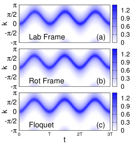
Figure 1: (Color online) Pair correlations functions as a function of momentum and time in the laboratory, reference frames, and zero-order Floquet approximation. In this plot, a $L=12$ sites chain has been simulated using $m=400$ DMRG states, $U=-4$ and $A/\omega=0.5$.

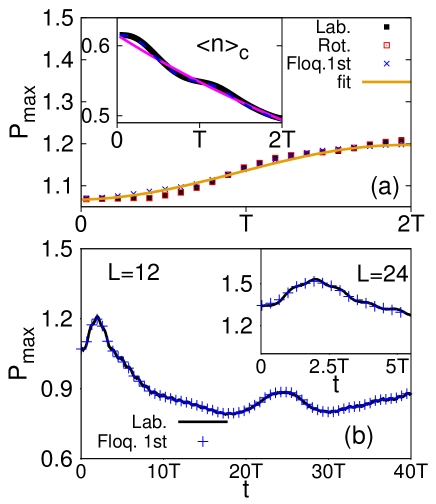
Figure 2: (Color online) Panel (a): magnitude of the condensate shown in the laboratory, rotating and Floquet first order approximation as a function of time. The solid (dark yellow) line indicates the fit $P_{max}=A+B\cos(Ct+D)$, as discussed in the main text. Inset: local density at the center of chain of length $L=12$ as a function of time (same filling and other parameters’ value as in fig. 1). Solid thick (black) line indicates data in the laboratory frame, the solid thin (magenta) line the data in the zero-order Floquet approximation, and the dashed (blue) line the data in the Floquet first order approximation. Panel (b): Long time behavior of the magnitude of the condensate. Notice the agreement between the laboratory frame and the Floquet approximation at first order. Inset: Magnitude of the condensate as a function of time for a system of length $L=24$, keeping up to $m=1000$ DMRG states with a maximum truncation error of $10^{-8}$.

The inset of panel (a) shows the local density at the center of chain of length $L=12$ as a function of time. The data in the laboratory frame (solid thick black line), which can be considered as an exact result, is compared with the zero and first order Floquet approximation (solid thin magenta and dashed blue lines, respectively). Even in the large frequency regime $J/\omega=0.05\ll 1$, one can see that the introduction of the kick operator at first order in the Floquet expansion is crucial to reproduce the out of equilibrium dynamics of the system within a single period of the external drive. Moreover, the results obtained in the laboratory frame and the first order Floquet approximation agree for all the times and system sizes investigated in this work. Indeed, panel (b) of fig. 2 studies the long time behaviour of the magnitude of the fermionic condensate for a larger system size chain showing a robust agreement between the two schemes. In both panels of fig. 2, we have retained up to $|m|=5$ harmonics in the expression of the kick operator in eq. (17).

Fig. 3 shows the pair correlation function for different values of the ratio $A/\omega$. One can notice that, by increasing the ratio $A/\omega$, the average position of the condensate peak moves towards the edge of the Brilloin zone. Eventually, it gets reflected at the boundary zone edge as displayed in Fig. 4b, where the average positions of the center of the condensate for small times $t\lesssim 5T$ are shown. By changing the driving parameters in the interval $0<A/\omega\lesssim 3$ one can tune the central peak of the Fermionic condensate in the entire Brilloin zone (see Fig. 4(b)). This effect demonstrates the possibility of tuning the average momentum of the condensate by changing the parameters of the external driving.

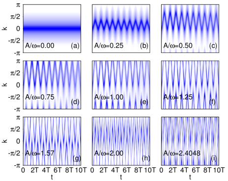
Figure 3: (Color online) Pair correlations functions as function of momentum and time calculated in the laboratory frame for different values of the ratio $A/\omega$. In this plot, a $L=12$ sites chain has been simulated using $m=400$ DMRG states, $U=-4$.

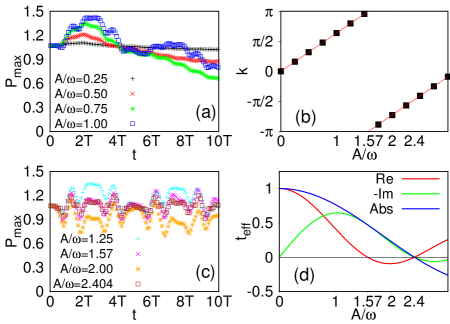
Figure 4: (Color online) Panels (a-c): Magnitude of the condensate shown in Fig. 3 as a function of time for different values of the ratio $A/\omega$. Panel (b): average position of the center-of-mass momentum of the condensate as a function of $A/\omega$ extracted from Fig. 3. The solid (red) line is a guide to the eye. Panel (d): Solid (red) line represent the real part of the hopping in the Floquet Hamiltonian in Eq. (13). Dashed (green) line is the imaginary part, short dashed (blue) line indicates its modulus. The line $y=0$ is drawn for convenience.

Panel (a) of Fig. 3 reproduces the trivial result for no driving as a reference. Focusing with more attention on the four panels (b-e), we find (not noticeable by eye) that the time-averaged position of the condensate in k-space at each period is not constant in time. The average momentum of the condensate is slowly reducing its amplitude as a function of the time. Correspondingly, we have studied the magnitude of the center-of-mass of the condensate as a function of time, which encodes the coherence of the Fermionic condensate. In Fig. 4(a) one can notice that, after an initial transient for times $t\lesssim 5T$, the coherence of the condensate decreases monotonically. This effect reaches its maximum for $A/\omega\simeq 0.75$. For larger driving amplitudes, the system builds up oscillations that survive at longer times, see the blue curve in Fig. 4(a). Interestingly, for a sufficiently large ratio of $A/\omega$, the oscillations of the magnitude of the condensate at large times are not suppressed anymore but are instead persistent, as shown in Fig. 4(c). In order to understand this behaviour, it is important to consider the effective description provided by the Floquet Hamiltonian. Fig. 4(d) shows real, imaginary and modulus of effective hopping parameter, $J_{eff}=JJ_{0}(z)e^{-iA/\omega}$, in the Floquet Hamiltonian in Eq. (13). We notice that the modulus of the effective hopping represents the well known renormalization of the electronic band structure due to the periodic driving, which can result in the dynamical fermionic localization at the zeros of the Bessel function $J_{0}(z)$. In the interval $1\lesssim A/\omega\lesssim 2.5$ the modulus of the effective hopping is significantly smaller than the other energy scale appearing in the Floquet Hamiltonian, the Coulomb repulsion $U$, $|J_{eff}|\ll U$. Interestingly, in this regime, the suppression of oscillations in the magnitude of the condensate are reduced, as seen in Fig. 4(c).

Fig. 5 presents the Fourier transform of the data shown in Fig. 4(a) and (c). Notice that the curves obtained for $A/\omega\leq 1$ in Fig. 4 are not time-periodic so the corresponding Fourier transforms shown in Fig. 5 present a low frequency peak, which simply reflects this slow decay. For larger driving amplitude $A/\omega=1.0$ one can notice emergence of two additional peaks at $\omega\pm U$ in the Fourier spectrum. The remaining curves of Fig. 5 are the Fourier transforms of the data shown in Fig. 4(c). Same as before, the main feature of the curves is the presence of the two peaks at $\omega\pm U$. Notice the appearance of the spectral peak at $\omega^{\prime}\simeq|U|$ together with a small contribution of two peaks at larger frequency corresponding to higher harmonics, $2\omega\pm U$. The contribution of high frequency harmonics is particularly significant at $A/\omega=2.4048$, where the absolute value of the effective hopping is zero, see Fig. 4(d).

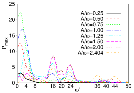
Figure 5: (Color online) Fourier transform of the curves shown in panel (a-c) of Fig. 4.

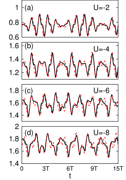
Figure 6: (Color online) Magnitude of the condensate for $A/\omega=2.4048$ and different values of the Coulomb repulsion $U$, as indicated. The red curves represent fits of the data according to the relation $P_{max}=A+B\sin(Ut)\sin(\omega t)$.

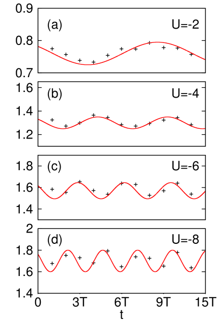
Figure 7: (Color online) Stroboscopic evolution of the magnitude of the condensate shown in Fig. 6. The red curves represent fits of the data according to the relation $P_{max}=A-B\sin(Ut+\phi)$.

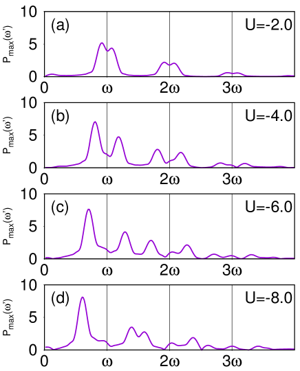
Figure 8: (Color online) Fourier transform of the curves shown in Fig. 6.

The results obtained can be interpreted as in Ref. [Bukov et al., 2016]. In fact, in the regime $U,\omega\gg J$, one can see that in a rotating frame defined by the canonical transformation $V(t)=e^{-i(f(t)\sum_{j}j{\hat{n}}_{j}+Ut\sum_{j}n_{\uparrow,j}n_{\downarrow,j})}$, the electron-electron interation $U$ induces non-trivial phase shifts in the hopping amplitude. Fig. 6 shows the magnitude of the condensate as a function of time for $A/\omega=2.4048$ for different values of the Coulomb repulsion $U$. Notice that an accurate fit of the data can be obtained using the relation $P_{max}=A+B\sin(Ut)\sin(\omega t)$, showing beats with frequencies $\omega\pm U$. The stroboscopic evolution at times equal to multiples of the period $T=2\pi/\omega$ of the driving perturbation is shown in Fig. 7. One can clearly observe that in a non-stroboscopic analysis, both the fast (the frequency of the driving force $\omega=20$) and the slow (the Coulomb repulsion $U$) time scales of the dynamics are resolved. A Fourier analysis of the data provides more details on the non-stroboscopic evolution, see Fig. 8. We find a clear contribution of at least three harmonics, with pairs of peaks at $n\omega\pm U$ (with $n=1,2,3$). For each pair, the distance between the two peaks is proportional to $2U$. The intensity of the Fourier peaks decreases almost exponentially with the order of the harmonics. Indeed, the zero-order Floquet expansion presented in the previous section for $A/\omega=2.4048$ corresponds to a Floquet Hamiltonian given just by the interaction term $H_{F}^{(0)}\simeq U\sum\limits_{i}n_{i,\sigma}n_{i,\bar{\sigma}}$. Therefore, this confirms that the zero-order Floquet approximation governs the stroboscopic long time evolution of the system.

In the next section, we will study the properties of the pairing states of the system in the laboratory reference frame by using different quench protocols.

IV Characterization of the pairing phase: quenching protocols

In this section we investigate the properties of the pairing phase by abruptly changing either the interactions, or the parameters of the periodic driving force. We first consider the quench protocol where we abruptly change the ratio $A/\omega$ of the driving but leaving the bare hopping and the $U$ attraction strength fixed. In practice, we change the values of the amplitude $A$ and keep the frequency of the driving fixed. In Fig. 9, we assume that before the quench $A_{1}/\omega=0.5$ while after the quench $A_{2}/\omega=2.4048$, which is the ratio corresponding to coherent destruction of tunnelling. In panels (a) and (b), the pair correlations functions are shown as a function of the momentum $k$ and the time $t$. In the panels (c) and (d) the magnitudes of the peaks at zero momentum are shown for $t=nT$, with $n$ non-negative integer. In panels (a) and (c), as also indicated by a vertical solid line, the quench is performed at $t=5T$, that is after exactly $5$ periods of the driving force. In panel (b) and (d), the quench is performed after $3.5$ periods of the driving. Panels (a) and (c) show a very interesting behaviour. If, in a real experiment, one is able to quench the amplitude of the driving at an instant of time that is an exact multiple of the driving frequency $\omega$, one would measure, in average, just a shift in the central peak of the pair distribution function, with no destruction of the condensate.

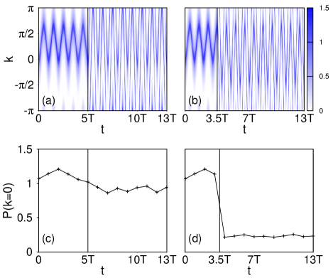
Figure 9: (Color online) Panels (a)-(b): Pair correlation functions before and after a quench of the amplitude of the driving from $A_{1}/\omega=0.5$ to $A_{2}/\omega=2.4048$. In panel (a) the quench is performed at $t=5T$, while in panel (b) at $t=3.5T$. Panels (c)-(d): Intensity of the peak at zero momentum of the same functions shown in panels (a) and (b) evaluated at each period of time $T$. In this plot, a $L=12$ sites chain has been simulated using $m=400$ DMRG states.

On the contrary, if a quench of the amplitude of the driving is done in any instant of time between $nT$ and $(n+1)T$ (we picked $3.5T$ as quenching time just for convenience), the oscillation of the peak of the condensate picks up a random phase factor which determines a significant (about 80%) suppression of the hight of the condensate peak (see panel (d)).

We now consider the possibility of quenching the interaction between the fermionic atoms loaded on the optical lattice. In panel (a) of Fig. 10, we assume that the fermionic condensate is initially prepared with $U_{1}=-8.0$ and with driving parameters given by the ratio $A_{1}/\omega=0.5$, such that the center of the condensate is around $k^{*}=1$ in average. At $t=5T$, we quench the interaction from $U=-8$ to zero, keeping the parameters of the driving fixed. After about a period of oscillation, the fermionic condensate is almost completely suppressed, because of the lost attraction between the fermions.

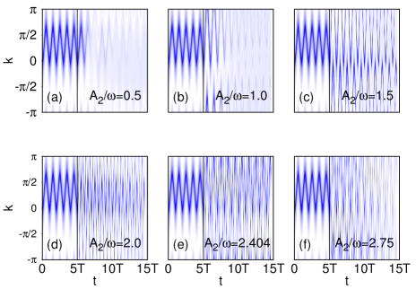
Figure 10: (Color online) Pair correlations functions as function of momentum and time for different values of the ratio $A_{2}/\omega$. A quench in the interaction from $U_{1}=-8$ to $U_{2}=0$ is performed at $t=5T$. For $t<5T$, $A_{1}/\omega=0.5$. In this plot, a $L=12$ sites chain has been simulated using $m=400$ DMRG states.

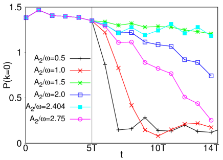
Figure 11: (Color online) Zero momentum contribution of the Pair correlations functions shown in Fig. 9 evaluated at each period of time $nT$, with $n=0,1,2,..,14$. In this plot, $A_{1}/\omega=0.5$ and $U_{1}=-8.0$.

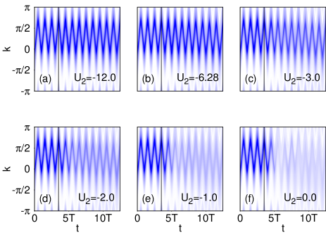
Figure 12: (Color online) Pair correlations functions before and after a quench at $t=3.5T$ of the interaction $U$. Initially, $U_{1}=-4.0$, while driving parameters are given by the ratio $A/\omega=0.5$. In this plot, a $L=12$ sites chain has been simulated using $m=400$ DMRG states.

A very non-trivial effect is visible if one increases the ratio $A_{2}/\omega$ after the quench: the coherence of the condensate displays revivals even if the bare interaction between the fermions is quenched to zero. A stroboscopic measure of the coherence of the condensate is provided in the panel (a) of Fig. 11. The revival of the coherence of the condensate is maximum around $A_{2}/\omega\simeq\pi/2$ and $A_{2}/\omega\simeq 2.4048$. All the other cases plotted, $A_{2}/\omega=1$, $A_{2}/\omega=2$, and $A_{2}/\omega=2.75$ show a decrease of the magnitude of the condensate peak. A qualitative explanation of the effects goes as follows: at the time of the quench, the effective Floquet Hamiltonian of the system changes accordingly with the new parameters of the driving. As demonstrated in Fig. 4(d), the real part of the effective hopping vanishes exactly at $A/\omega\simeq\pi/2$ and $A/\omega\simeq 2.4048$. As shown in Ref. [Creffield and Sols, 2011] the real part of the effective hopping is proportional to the spreading of a condensate prepared in real space, which is then let evolved in time under the action of the driving.

We finally address a peculiar quenching protocol where we keep the parameters of the driving fixed and, after preparing the condensate with a finite average center-of-mass momentum, we quench the attraction strength at time $t=3.5T$ (as indicated by the black vertical line). Results are shown in Fig. 12. If the strength of the attraction between fermions is quenched to a value which is larger in modulus than the initial value $U=-4$ (see panels for $U_{2}=-12$ and $U_{2}=-6.28$), the center-of-mass momentum does not change, while the magnitude of the condensate peak is increased (not shown in the plot). If the modulus of the strength of the attraction between the fermions is decreased, not only the coherence of the condense decreases, going to zero if $U_{2}=0$, but the average center-of-mass momentum also drifts toward zero (see panels for $U_{2}=-2$ and $U_{2}=-1$).

V CONCLUSIONS

In this work, we have studied the one-dimensional attractive Fermionic Hubbard model subjected to a sinusoidal periodic drive. We have assumed that the frequency of the driving force is large enough such that the system is in the off-resonant regime, and Floquet theory can be applied. To benchmark our numerical simulations, we have verified that a Van Vleck high-frequency expansion in the rotating frame truncated to first order is able to describe very well the numerical results obtained with time dependent DMRG. In particular, at zero order, the stroboscopic dynamics in a rotated reference frame is described by an effective Floquet Hamiltonian with a complex phase in the hopping term which introduces a shift of the condensate center-of-mass momentum. We have also derived the micromotion or kick operators and verified that their inclusion at first order of the high-frequency expansion is crucial to understand the dynamics of the system within one period of the external drive.

By tuning the amplitude and the frequency of the driving force, one can realize an unconventional Fermionic condensate with a finite center-of-mass momentum. This pairing state is similar to a FF state, because it represents a coherent matter field of Cooper-like pairs at finite momentum. In particular, the center-of-mass of the condensate can be tuned at will across the Brilloin zone. Moreover, we have shown that the coherence of the condensate, which is encoded in the magnitude of the pair correlation function in momentum space, can be enhanced by tuning the amplitude and frequency of the drive to ratios close to those where one obtains fermionic dynamical localization.

From the analysis of the real time evolution of the magnitude of the condensate, we found that the stroboscopic dynamics is governed by oscillations with period proportional to the electron-electron attraction strength $U$, while the full time evolution presents also oscillations given by the driving frequency $\omega$, creating beats at $\omega\pm U$.

Finally, we show that using different quenching protocols, the condensate can be frozen at a particular finite center-of-mass momentum and coherence. Moreover, the coherence of the condensate displays revivals even if the bare interaction between the fermions is quenched to zero. These protocols are within experimental reach.

Our work could pave the way for engineering out-of equilibrium FFLO-like phases in multicomponent Fermi gases without population imbalance.

VI ACKNOWLEDGMENTS

This work was conducted at the Center for Nanophase Materials Sciences, sponsored by the Scientific User Facilities Division (SUFD), Basic Energy Sciences (BES), U.S. Department of Energy (DOE), under contract with UT-Battelle. A.N. acknowledges support by the Center for Nanophase Materials Sciences, and by the Early Career Research program, SUFD, BES, DOE. A.E.F. acknowledges the DOE, Office of Basic Energy Sciences, for support under grant DE-SC0014407. A.P. was supported by NSF DMR-1506340, ARO W911NF1410540 and AFOSR FA9550-16-1-0334.

References

- Bloch et al. (2008) I. Bloch, J. Dalibard, and W. Zwerger, Rev. Mod. Phys. 80, 885 (2008), URL http://link.aps.org/doi/10.1103/RevModPhys.80.885.
- Lewenstein et al. (2012) M. Lewenstein, A. Sanpera, and V. Ahufinger, Ultracold Atoms in Optical Lattices: Simulating quantum many-body systems (Oxford University Press Oxford, 2012).
- Buluta and Nori (2009) I. Buluta and F. Nori, Science 326, 108 (2009).
- Bloch et al. (2012) I. Bloch, J. Dalibard, and S. Nascimbène, Nature Physics 8, 267 (2012).
- Georgescu et al. (2014) I. M. Georgescu, S. Ashhab, and F. Nori, Rev. Mod. Phys. 86, 153 (2014), URL http://link.aps.org/doi/10.1103/RevModPhys.86.153.
- Bakr et al. (2010) W. S. Bakr, A. Peng, M. E. Tai, R. Ma, J. Simon, J. I. Gillen, S. Foelling, L. Pollet, and M. Greiner, Science 329, 547 (2010).
- Sherson et al. (2010) J. F. Sherson, C. Weitenberg, M. Endres, M. Cheneau, I. Bloch, and S. Kuhr, Nature 467, 68 (2010).
- Jaksch and Zoller (2003) D. Jaksch and P. Zoller, New Journal of Physics 5, 56 (2003).
- Lin et al. (2009) Y.-J. Lin, R. L. Compton, K. Jiménez-García, J. V. Porto, and I. B. Spielman, Nature 462, 628 (2009).
- Dalibard et al. (2011) J. Dalibard, F. Gerbier, G. Juzeliūnas, and P. Öhberg, Rev. Mod. Phys. 83, 1523 (2011), URL http://link.aps.org/doi/10.1103/RevModPhys.83.1523.
- Struck et al. (2012) J. Struck, C. Ölschläger, M. Weinberg, P. Hauke, J. Simonet, A. Eckardt, M. Lewenstein, K. Sengstock, and P. Windpassinger, Phys. Rev. Lett. 108, 225304 (2012), URL http://link.aps.org/doi/10.1103/PhysRevLett.108.225304.
- Lignier et al. (2007) H. Lignier, C. Sias, D. Ciampini, Y. Singh, A. Zenesini, O. Morsch, and E. Arimondo, Phys. Rev. Lett. 99, 220403 (2007), URL http://link.aps.org/doi/10.1103/PhysRevLett.99.220403.
- Zenesini et al. (2009) A. Zenesini, H. Lignier, D. Ciampini, O. Morsch, and E. Arimondo, Phys. Rev. Lett. 102, 100403 (2009), URL http://link.aps.org/doi/10.1103/PhysRevLett.102.100403.
- Winkler et al. (2006) K. Winkler, G. Thalhammer, F. Lang, R. Grimm, J. H. Denschlag, A. Daley, A. Kantian, H. Büchler, and P. Zoller, Nature 441, 853 (2006).
- Eckardt et al. (2005) A. Eckardt, C. Weiss, and M. Holthaus, Physical review letters 95, 260404 (2005).
- Di Liberto et al. (2011) M. Di Liberto, O. Tieleman, V. Branchina, and C. M. Smith, Phys. Rev. A 84, 013607 (2011), URL http://link.aps.org/doi/10.1103/PhysRevA.84.013607.
- Creffield and Sols (2008) C. E. Creffield and F. Sols, Phys. Rev. Lett. 100, 250402 (2008), URL http://link.aps.org/doi/10.1103/PhysRevLett.100.250402.
- Creffield and Sols (2011) C. E. Creffield and F. Sols, Phys. Rev. A 84, 023630 (2011), URL http://link.aps.org/doi/10.1103/PhysRevA.84.023630.
- Zwierlein et al. (2006) M. W. Zwierlein, A. Schirotzek, C. H. Schunck, and W. Ketterle, Science 311, 492 (2006).
- Partridge et al. (2006) G. B. Partridge, W. Li, R. I. Kamar, Y.-a. Liao, and R. G. Hulet, Science 311, 503 (2006).
- Liao et al. (2010) Y.-a. Liao, A. S. C. Rittner, T. Paprotta, W. Li, G. B. Partridge, R. G. Hulet, S. K. Baur, and E. J. Mueller, Nature 467, 567 (2010).
- Orso (2007) G. Orso, Phys. Rev. Lett. 98, 070402 (2007), URL http://link.aps.org/doi/10.1103/PhysRevLett.98.070402.
- Feiguin and Heidrich-Meisner (2007) A. E. Feiguin and F. Heidrich-Meisner, Phys. Rev. B 76, 220508 (2007), URL http://link.aps.org/doi/10.1103/PhysRevB.76.220508.
- Casula et al. (2008) M. Casula, D. M. Ceperley, and E. J. Mueller, Phys. Rev. A 78, 033607 (2008), URL http://link.aps.org/doi/10.1103/PhysRevA.78.033607.
- Lüscher et al. (2008) A. Lüscher, R. M. Noack, and A. M. Läuchli, Phys. Rev. A 78, 013637 (2008), URL http://link.aps.org/doi/10.1103/PhysRevA.78.013637.
- Rizzi et al. (2008) M. Rizzi, M. Polini, M. A. Cazalilla, M. R. Bakhtiari, M. P. Tosi, and R. Fazio, Phys. Rev. B 77, 245105 (2008), URL http://link.aps.org/doi/10.1103/PhysRevB.77.245105.
- Tezuka and Ueda (2008) M. Tezuka and M. Ueda, Phys. Rev. Lett. 100, 110403 (2008), URL http://link.aps.org/doi/10.1103/PhysRevLett.100.110403.
- Feiguin et al. (2012) A. Feiguin, F. Heidrich-Meisner, G. Orso, and W. Zwerger, in The BCS-BEC Crossover and the Unitary Fermi Gas (Springer, 2012), pp. 503–532.
- Guan et al. (2013) X.-W. Guan, M. T. Batchelor, and C. Lee, Rev. Mod. Phys. 85, 1633 (2013), URL http://link.aps.org/doi/10.1103/RevModPhys.85.1633.
- Fulde and Ferrell (1964) P. Fulde and R. A. Ferrell, Phys. Rev. 135, A550 (1964), URL http://link.aps.org/doi/10.1103/PhysRev.135.A550.
- Larkin and Ovchinnikov (1964) A. I. Larkin and Y. N. Ovchinnikov, Zh. Eksp. Teor. Fiz. 47 (1964).
- Yang (2001) K. Yang, Phys. Rev. B 63, 140511 (2001), URL http://link.aps.org/doi/10.1103/PhysRevB.63.140511.
- Casalbuoni and Nardulli (2004) R. Casalbuoni and G. Nardulli, Rev. Mod. Phys. 76, 263 (2004), URL http://link.aps.org/doi/10.1103/RevModPhys.76.263.
- Bukov and Polkovnikov (2014a) M. Bukov and A. Polkovnikov, Phys. Rev. A 90, 043613 (2014a), URL http://link.aps.org/doi/10.1103/PhysRevA.90.043613.
- Bukov and Polkovnikov (2014b) M. Bukov and A. Polkovnikov, Phys. Rev. A 90, 043613 (2014b), URL http://link.aps.org/doi/10.1103/PhysRevA.90.043613.
- Eckardt and Anisimovas (2015) A. Eckardt and E. Anisimovas, New Journal of Physics 17, 093039 (2015), URL http://stacks.iop.org/1367-2630/17/i=9/a=093039.
- Bukov et al. (2015) M. Bukov, L. D’Alessio, and A. Polkovnikov, Advances in Physics 64, 139 (2015), eprint http://dx.doi.org/10.1080/00018732.2015.1055918, URL http://dx.doi.org/10.1080/00018732.2015.1055918.
- Mikami et al. (2016) T. Mikami, S. Kitamura, K. Yasuda, N. Tsuji, T. Oka, and H. Aoki, Phys. Rev. B 93, 144307 (2016), URL http://link.aps.org/doi/10.1103/PhysRevB.93.144307.
- White and Feiguin (2004a) S. R. White and A. E. Feiguin, Phys. Rev. Lett. 93, 076401 (2004a), URL http://link.aps.org/doi/10.1103/PhysRevLett.93.076401.
- Daley et al. (2004) A. J. Daley, C. Kollath, U. Schollwöck, and G. Vidal, Journal of Statistical Mechanics: Theory and Experiment 2004, P04005 (2004), URL http://stacks.iop.org/1742-5468/2004/i=04/a=P04005.
- White and Feiguin (2004b) S. R. White and A. E. Feiguin, Phys. Rev. Lett. 93, 076401 (2004b), URL http://link.aps.org/doi/10.1103/PhysRevLett.93.076401.
- Bukov et al. (2016) M. Bukov, M. Kolodrubetz, and A. Polkovnikov, Phys. Rev. Lett. 116, 125301 (2016), URL http://link.aps.org/doi/10.1103/PhysRevLett.116.125301.