Magnetic field sensing with quantum error detection under the effect of energy relaxation

Abstract

A solid state spin is an attractive system with which to realize an ultra-sensitive magnetic field sensor. A spin superposition state will acquire a phase induced by the target field, and we can estimate the field strength from this phase. Recent studies have aimed at improving sensitivity through the use of quantum error correction (QEC) to detect and correct any bit-flip errors that may occur during the sensing period. Here, we investigate the performance of a two-qubit sensor employing QEC and under the effect of energy relaxation. Surprisingly, we find that the standard QEC technique to detect and recover from an error does not improve the sensitivity compared with the single-qubit sensors. This is a consequence of the fact that the energy relaxation induces both a phase-flip and a bit-flip noise where the former noise cannot be distinguished from the relative phase induced from the target fields. However, we have found that we can improve the sensitivity if we adopt postselection to discard the state when error is detected. Even when quantum error detection is moderately noisy, and allowing for the cost of the postselection technique, we find that this two-qubit system shows an advantage in sensing over a single qubit in the same conditions.

Measurement of small magnetic fields is an important objective in the field of metrology because of many practical applications in material science, biology, and medical science. It is known that SQUID Simon (1999), Hall sensors Chang et al. (1992), and force sensors Poggio and Degen (2010) show excellent performance for such field detection.

A two-level system coupled with magnetic fields is an alternative way to detect small magnetic field. The magnetic field typically shifts the resonant frequency of the qubit, and one can readout the shift from Ramsey type interference experiment, to which we refer as single-qubit sensors. Atomic vapor magnetometry is one of such ways to use a qubit for sensing Budker and Romalis (2007). Nitrogen vacancy centers in diamond is another candidate to realize such a sensor Maze et al. (2008); Taylor et al. (2008); Balasubramanian et al. (2008), and this typically has a better spatial resolution compared with other conventional devices.

One of the obstacles to sense small magnetic fields with the qubit is decoherence on the system Huelga et al. (1997). The frequency shift from the magnetic fields induces a relative phase between coherent superpositions of the qubit, and this provides us with measurable signals Degen et al. (2016). This means that any deteriorating effect of the phase coherence decreases the signal to noise ratio of the sensing. Since unwanted coupling with environment is inevitable, the decoherence effect is one of the main challenges to realize an ultra-sensitive field sensor with qubits.

Recently, magnetic field sensing with quantum error correction (QEC) has been proposed to improve the sensitivity of qubit-based metrology Kessler et al. (2014); Arrad et al. (2014); Dür et al. (2014); Herrera-Martí et al. (2015). QEC is a technique to detect and recover errors by using an encoded state where ancillary qubits are used to employ redundancy in the code space Gottesman (2009). QEC has been proposed in the context of scalable quantum computation, and proof of principle experiments have been demonstrated in many systems such as superconducting qubits Gladchenko et al. (2009); Reed et al. (2012); Córcoles et al. (2015); Kelly et al. (2015), NV centers Waldherr et al. (2014), and ion traps Nigg et al. (2014). Moreover, previous researches show that QEC can be applied to enhance the sensitivity in the quantum metrology with certain conditions Kessler et al. (2014); Arrad et al. (2014). Interestingly, even for a two-qubit system, it is in principle possible to enhance the sensitivity by QEC if one of the qubits has much longer coherence time than the other Kessler et al. (2014); Arrad et al. (2014). It is worth mentioning that we should not apply QEC to protect the qubit from the dephasing during the sensing, because the relative phase from the target magnetic field is indistinguishable from the unwanted phase induced by the environment. On the other hand, if a bit-flip noise is relevant on the qubits, quantum field sensors with QEC can beat the single-qubit sensors Kessler et al. (2014); Arrad et al. (2014); Dür et al. (2014). Indeed, an experiment has been reported where such an enhancement of the sensitivity by QEC was demonstrated under the effect of artificial bit-flip noise by using a nitrogen vacancy center in diamond or an optical setup Unden et al. (2016); Cohen et al. (2016). However, to our knowledge there has not yet been any experimental demonstration of the enhancement of the sensitivity of quantum metrology by QEC versus natural decoherence from the environment.

In this paper, we investigate the performance of the quantum field sensing with QEC technique under the effect of energy relaxation. A solid state spin qubit is affected by two type of decoherence, dephasing and energy relaxation. The dephasing time of the qubit is characterized by $T_{2}$ while the energy relaxation time is characterized by $T_{1}$ Slichter (2013). It is worth mentioning that dynamical decoupling techniques are available to suppress the effect of the dephasing, which can improve the sensitivity for AC magnetic fields Viola et al. (1999); Taylor et al. (2008). With a well-controlled dynamical decoupling technique, the coherence time of the solid state qubit can be in principle limited by the energy relaxation process, which is observed in several systems such as superconducting qubits Bylander et al. (2011); Yan et al. (2015). However, the energy relaxation induces not only bit-flip noise but also phase-flip noise. As pointed out in Kessler et al. (2014); Arrad et al. (2014); Dür et al. (2014), QEC versus dephasing cannot be applied to enhance the sensitivity of quantum metrology, because QEC erases not only the environmental unknown phase but also the relative phase induced by the target fields. So it is not trivially obvious if QEC can improve the sensitivity if the energy relaxation is a relevant source of the decoherence. Here we investigate the performance of quantum field sensors using QEC, where the error is detected and recovered on the encoded state with an ancillary qubit. We show that the standard QEC approach does not improve the sensitivity over the single-qubit sensors. We proceed to consider a postselection strategy where we discard the state when the bit-flip error is detected. Since we need to wait until we have successful operations, the postselection effectively decrease the time resource. Interestingly, even if we take into account the time loss due to the postselection, we show that such a postselection strategy actually improves the sensitivity, and beats single-qubit sensors. Moreover, this is true even when the detection process is imperfect and can itself introduce noise. Our results show that an encoded two-qubit state is actually beneficial for ultra-sensitive magnetic field sensing in realistic conditions.

I Magnetic field sensing with the standard Ramsey type sequence

Let us review the standard Ramsey type sequence to estimate the magnetic fields with a qubit Huelga et al. (1997), which we refer to as single-qubit sensors. Suppose that we have a qubit coupled with magnetic field, and the Hamiltonian is described by

$$H=\frac{\omega}{2}\hat{\sigma}_{z}$$ (1)

where $\omega$ denotes a detuning due to the magnetic field $B$, and we assume that the detuning has a linear relationship with the magnetic field. Firstly, we prepare $|+\rangle=\frac{1}{\sqrt{2}}(|0\rangle+|1\rangle)$. Secondly, let this state evolve under the Hamiltonian for a time $t$, and we obtain $\frac{1}{\sqrt{2}}(e^{-i\frac{\omega}{2}t}|0\rangle+e^{i\frac{\omega}{2}t}|1\rangle)$. Finally, we perform a projective measurement about $\hat{\sigma}_{y}$ on this state, and we project this state into $|+_{y}\rangle=\frac{1}{\sqrt{2}}(|0\rangle+i|1\rangle)$ with a probability of $P_{+1}=\frac{1}{2}+\frac{1}{2}\sin\omega t$. Throughout of this paper, we assume that the magnetic field is weak ($\omega t\ll 1$), and so we have $P_{+1}\simeq\frac{1}{2}+\frac{1}{2}\omega t$. By repeating this experiment many times, we can obtain the probability from the experimental results and so the value of $\omega$ can be estimated. The uncertainty of the estimation is given by

$$\delta\omega=\frac{\sqrt{P_{+1}(1-P_{+1})}}{|\frac{dP_{+1}}{d\omega}|}\frac{1}{\sqrt{N}}$$ (2)

where $N$ denotes the number of repetitions of the experiments Huelga et al. (1997). We assume that the interaction time $t$ is much longer than the state preparation time and measurement readout time. In this case, we have $N\simeq\frac{T}{t}$ where $T$ is a given time for the sensing. We can calculate the uncertainty as

$$\delta\omega\simeq\frac{1}{\sqrt{Tt}}$$ (3)

We consider the magnetic field sensing under the effect of energy relaxation. The energy relaxation can be described by the standard Lindblad type master equation as Lindblad (1976); Hornberger (2009)

$$\frac{d\rho(t)}{dt}=-i[H,\rho(t)]$$ (4)

$$- \frac{2\Gamma(1-s)}{2}(\sigma_{+}\sigma_{-}\rho(t)+\rho(t)\hat{\sigma}_{+}\sigma_{-}-2\sigma_{-}\rho(t)\sigma_{+})$$

$$- \frac{2\Gamma s}{2}(\sigma_{-}\sigma_{+}\rho(t)+\rho(t)\hat{\sigma}_{-}\sigma_{+}-2\sigma_{+}\rho(t)\sigma_{-})$$

Here, $\Gamma$ denotes a decay rate while $s$ depends on the temperature of the bath where $s=\frac{1}{2}$ ($s=0$) corresponds to an infinite (a zero) temperature Gardiner and Zoller (2004). An analytical solution for this master equation is given as Hein et al. (2005)

$$\rho_{I}(t)=\frac{1}{4}(1+2e^{-\Gamma t}+e^{-2\Gamma t})\rho_{0}+\frac{1}{4}(1-e^{-2\Gamma t})\hat{\sigma}_{x}\rho_{0}\hat{\sigma}_{x}$$

$$+\frac{1}{4}(1-e^{-2\Gamma t})\hat{\sigma}_{y}\rho_{0}\hat{\sigma}_{y}+\frac{1}{4}(1-2e^{-\Gamma t}+e^{-2\Gamma t})\hat{\sigma}_{z}\rho_{0}\hat{\sigma}_{z}$$

$$+\frac{2s-1}{4}(1-e^{-2\Gamma t})(\hat{\sigma}_{z}\rho_{0}+\rho_{0}\hat{\sigma}_{z}-i\hat{\sigma}_{x}\rho_{0}\hat{\sigma}_{y}+i\hat{\sigma}_{y}\rho_{0}\hat{\sigma}_{x})$$ (5)

where $\rho_{I}(t)=e^{iHt}\rho(t)e^{-iHt}$ and $\rho_{0}=\rho(0)$. In the Ramsey type sequence with the energy relaxation, we obtain

$$P_{+1}={\rm{Tr}}[|+_{y}\rangle\langle+_{y}|\rho(t)]$$ (6)

$$= \frac{1}{2}+\frac{1}{2}e^{-\Gamma t}\sin\omega t\simeq\frac{1}{2}+\frac{1}{2}e^{-\Gamma t}\omega t.$$

For the weak magnetic fields, we can calculate the uncertainty from Eq. (2) as

$$\delta\omega\simeq\frac{2.33}{\sqrt{T/\Gamma}}$$ (7)

where we choose an optimum $t$ to minimize the uncertainty.

II Magnetic field sensing with quantum error correction

We adopt a strategy to use the standard quantum error correction technique for the magnetic field sensing suggested in Kessler et al. (2014); Arrad et al. (2014); Dür et al. (2014). This requires two distinct qubits, namely a probe qubit and a memory qubit. The probe qubit is coupled with the magnetic field, while the interaction of the memory qubit with the magnetic field is negligible. On the other hand, the probe qubit is affected by energy relaxation while the memory qubit has a much longer coherence time than the probe qubit. Also, we assume that, on these two qubits, we can implement any unitary operations and measurements with a much shorter time scale than the coherence time of the qubits.

The Hamiltonian is described as

$$H=\frac{\omega}{2}\hat{\sigma}_{z}^{{\rm{(p)}}}+\frac{\omega^{\prime}}{2}\hat{\sigma}_{z}^{{\rm{(m)}}}$$ (8)

where $\omega$ ($\omega^{\prime}$) denotes the resonant frequency of the probe (memory) qubit. We assume $\omega\gg\omega^{\prime}$, and so we use an approximation to drop the term of $\frac{\omega^{\prime}}{2}\hat{\sigma}_{z}^{{\rm{(m)}}}$ from the Hamiltonian. Also, the Lindblad master equation is described as

$$\frac{d\rho(t)}{dt}=-i[H,\rho(t)]$$ (9)

$$- \frac{2\Gamma(1-s)}{2}(\sigma_{+}^{\rm{(p)}}\sigma^{\rm{(p)}}_{-}\rho(t)+\rho(t)\hat{\sigma}^{\rm{(p)}}_{+}\sigma^{\rm{(p)}}_{-}-2\sigma^{\rm{(p)}}_{-}\rho(t)\sigma^{\rm{(p)}}_{+})$$

$$- \frac{2\Gamma s}{2}(\sigma^{\rm{(p)}}_{-}\sigma^{\rm{(p)}}_{+}\rho(t)+\rho(t)\hat{\sigma}^{\rm{(p)}}_{-}\sigma^{\rm{(p)}}_{+}-2\sigma^{\rm{(p)}}_{+}\rho(t)\sigma^{\rm{(p)}}_{-})\ \$$

where only a probe qubit is affected by the energy relaxation.

II.1 Parity measurement

To demonstrate magnetic field sensing with quantum error correction (QEC), parity measurements are necessary to detect bit flip errors Kessler et al. (2014); Arrad et al. (2014); Dür et al. (2014); Herrera-Martí et al. (2015), and we describe how we can construct the parity measurement by using the two-qubit system without additional ancillary qubits. We define a controlled-not (CNOT) gate as follows

$$U_{\rm{CNOT}}=|0\rangle_{\rm{p}}\langle 0|\otimes\hat{\openone}_{\rm{m}}+|1\rangle_{\rm{p}}\langle 1|\otimes\hat{\sigma}^{({\rm{m}})}_{x}$$ (10)

where the probe (memory) qubit is the control (target). By performing the CNOT gate, a projective measurement in the basis of $\hat{\sigma}_{z}^{({\rm{m}})}$, and another CNOT gate, we can construct the following projective measurements.

$$\hat{\mathcal{P}}_{\rm{odd}}=U_{\rm{CNOT}}\frac{\hat{\openone}+\hat{\sigma}^{({\rm{m}})}_{z}}{2}U_{\rm{CNOT}}=|01\rangle_{\rm{pm}}\langle 01|+|10\rangle_{\rm{pm}}\langle 10|$$

$$\hat{\mathcal{P}}_{\rm{even}}=U_{\rm{CNOT}}\frac{\hat{\openone}-\hat{\sigma}^{({\rm{m}})}_{z}}{2}U_{\rm{CNOT}}=|00\rangle_{\rm{pm}}\langle 00|+|11\rangle_{\rm{pm}}\langle 11|$$

and these are called parity measurements.

II.2 Single quantum error correction cycle

By using this system, we can implement quantum field sensing as follows. Let us consider a case when we implement the QEC cycle only one time. Firstly, we prepare a state $\rho_{0}=|\phi_{0}\rangle_{\rm{pm}}\langle\phi_{0}|$ where $|\phi_{0}\rangle_{\rm{pm}}=\frac{1}{\sqrt{2}}(|00\rangle_{{\rm{pm}}}+|11\rangle_{{\rm{pm}}})$. Secondly, let this state evolve by the Lindblad master equation in Eq. (9) for a time $t$. Thirdly, we perform a parity projection to check if a bit-flip error occurs on the probe qubit. If the parity is even (odd), a projective operator described by $\hat{\mathcal{P}}_{{\rm{even}}}=|00\rangle_{\rm{pm}}\langle 00|+|11\rangle_{\rm{pm}}\langle 11|$ ($\hat{\mathcal{P}}_{{\rm{odd}}}=|01\rangle_{\rm{pm}}\langle 01|+|10\rangle_{\rm{pm}}\langle 10|$) is applied on the quantum states. If the parity is odd, this provides us with the existence of the bit-flip error on the probe qubit, and so we will apply a recovery operation $\hat{\sigma}_{x}^{(\rm{p})}$ on the probe qubit. Finally, we measure the state in the basis of $|\psi^{(\pm)}_{\rm{f}}\rangle_{{\rm{pm}}}=\frac{1}{\sqrt{2}}(|00\rangle_{{\rm{pm}}}\pm i|11\rangle_{{\rm{pm}}})$ where the projection operator is described as $\hat{\mathcal{P}}^{{\rm{(pm)}}}_{{{\rm{f}}},\pm}=|\psi^{(\pm)}_{\rm{f}}\rangle_{{\rm{pm}}}\langle\psi^{(\pm)}_{\rm{f}}|$. In this case, the readout probability can be calculated as

$$P^{({\rm{QEC}})}_{+1}={\rm{Tr}}[\hat{\mathcal{P}}^{{\rm{(pm)}}}_{{{\rm{f}}},+}\rho^{{\rm{(QEC)}}}(t)]=\frac{1}{2}+\frac{1}{2}e^{-\Gamma t}\sin\omega t.$$ (11)

Interestingly, this is the same probability as the Eq. (6), and so the uncertainty of the estimation with QEC is the same as that of the single-qubit sensors.

II.3 Multiple quantum error correction cycle

Let us consider a case when we implement multiple QEC cycles. The first step is to prepare a state $\frac{1}{\sqrt{2}}(|00\rangle_{{\rm{pm}}}+|11\rangle_{{\rm{pm}}})$. The second step is a time evolution of the system by the Lindblad master equation in Eq. (4) for a time $\tau=t/n$ where $n$ denotes the number of the parity measurements. The third step is to perform a parity projection. If the parity is odd, we will apply the recovery operation $\hat{\sigma}_{x}^{(\rm{p})}$ on the probe qubit. The final step is that, after repeating the second step and the third step $n$ times, we readout the state via the measurement in the basis of $\frac{1}{\sqrt{2}}(|00\rangle_{{\rm{pm}}}\pm i|11\rangle_{{\rm{pm}}})$ where the projective operator is described as $\hat{\mathcal{P}}^{{\rm{(pm)}}}_{\pm 1}=\frac{1}{2}(|00\rangle_{{\rm{pm}}}\pm i|11\rangle_{{\rm{pm}}})(\langle 00|\pm i{}_{{\rm{pm}}}\langle 11|)$. We numerically calculate the uncertainty $\delta\omega$ for this protocol, and plot it in the Fig 1. Interestingly, $\delta\omega$ does not depend on $n$, and the implementation of the multiple QEC does not improve the sensitivity over the standard Ramsey type scheme. Although we plot the case of $s=0.5$ in the Fig 1, we obtain the same results for other values of $s$.

Let us discuss a possible reason why QEC does not improve the sensitivity. For simplicity, we specifically discuss the case for $s=0.5$. From Eq. (5), we know that the qubit is affected by three types of Pauli noise, namely $\hat{\sigma}_{x}$, $\hat{\sigma}_{y}$, and $\hat{\sigma}_{z}$. Importantly, since the initial state is an eigenstate of $\hat{\sigma}_{x}$, consequently it is $\hat{\sigma}_{y}$ and $\hat{\sigma}_{z}$ errors mainly decohere the qubit. On the other hand, if we use the two-qubit encoded state, then $\hat{\sigma}^{(\rm{p})}_{x}$, $\hat{\sigma}^{(\rm{p})}_{y}$, and $\hat{\sigma}^{(\rm{p})}_{z}$ all induce decoherence. Moreover, QEC with the two-qubit code cannot distinguish the error of $\hat{\sigma}^{(\rm{p})}_{x}$ from the error of $\hat{\sigma}^{(\rm{p})}_{y}$, and so the recovery operation can remove only one of these two errors. Therefore, even if we implement QEC, two types of error still remains in the quantum states, which is effectively the same as the case of the single-qubit strategy. This qualitatively explains why QEC cannot improve the sensitivity for the metrology under the effect of energy relaxation.

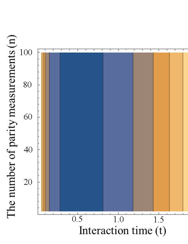
Figure 1: Uncertainty of the estimation of the magnetic fields with multiple QEC cycles under the effect of energy relaxation. The parameters are chosen as $s=0.5$ and $\Gamma=1$. We use two qubits to construct an encoded state, and one of the qubits is affected by energy relaxation. By performing parity measurements with a time period of $\frac{t}{n}$ where $t$ denotes a total evolution time and $n$ denotes the number of the parity measurements, we can detect the bit flip error, and the subsequent bit-flip operation can recover the state. However, these numerical results show that the uncertainty does not depend on $n$, and so we cannot improve the sensitivity even if we increase the number of QEC cycles. The minimum uncertainty is still 2.33, as with the single-qubit sensor.

III Magnetic field sensing with quantum error detection

Here, we propose to use a postselection where we discard the state when we detect the bit-flip error, which we refer to as a quantum error detection (QED) strategy. As with the QEC strategy, we will use two different systems, namely a probe qubit and a memory qubit so that we can encode the state in a logical basis. Surprisingly, we will show that this postselection actually provides us with quantum enhancement over the single-qubit sensors.

III.1 Single quantum error detection

Let us discuss the case where we implement the QED only one time. In QED strategy, we use the same sequence as QEC except that we discard the state when the error is detected by the parity projection. The final state before the measurement readout is calculated as

$$\rho^{{\rm{(QED)}}}(t)=\frac{1}{(\frac{1+e^{-2\Gamma t}}{2})}e^{-iHt}\Big{(}\frac{1}{4}(1+2e^{-\Gamma t}+e^{-2\Gamma t})\rho_{0}$$

$$+\frac{1}{4}(1-2e^{-\Gamma t}+e^{-2\Gamma t})\hat{\sigma}^{(\rm{p})}_{z}\rho_{0}\hat{\sigma}^{(\rm{p})}_{z}$$

$$+\frac{2s-1}{4}(1-e^{-2\Gamma t})(\hat{\sigma}^{(\rm{p})}_{z}\rho_{0}+\rho_{0}\hat{\sigma}^{(\rm{p})}_{z})\Big{)}e^{iHt}$$

where the success probability to obtain this state is $\frac{1+e^{-2\Gamma t}}{2}$. The probability to project this state into $\hat{\mathcal{P}}^{{\rm{(pm)}}}_{{{\rm{f}}},+}$ is calculated as

$$P^{({\rm{QED}})}_{+1}={\rm{Tr}}[\hat{\mathcal{P}}^{{\rm{(pm)}}}_{{{\rm{f}}},+}\rho^{{\rm{(QED)}}}(t)]=\frac{1}{2}+\frac{1}{2}\frac{\sin\omega t}{(\frac{e^{\Gamma t}+e^{-\Gamma t}}{2})}$$ (12)

and so the uncertainty is given as

$$\delta\omega\simeq\frac{e^{\Gamma t}+e^{-\Gamma t}}{2t}\frac{1}{\sqrt{N}}=\sqrt{\frac{e^{2\Gamma t}+1}{2}}\frac{1}{\sqrt{Tt}}$$ (13)

where $N\simeq\sqrt{\frac{T}{t}\frac{1+e^{-2\Gamma t}}{2}}$ denotes the number of the measurement readouts when no error is detected. For weak magnetic fields, we obtain

$$\delta\omega\simeq\frac{1.895}{\sqrt{T/\Gamma}}$$ (14)

where we choose $t$ to minimize $\delta\omega$, and this show that the QED strategy is better than the single-qubit sensors.

Let us discuss a possible reason why the QED can improve the sensitivity. The probe qubit is affected by three type of Pauli noise, namely $\hat{\sigma}^{(\rm{p})}_{x}$, $\hat{\sigma}^{(\rm{p})}_{y}$, and $\hat{\sigma}^{(\rm{p})}_{z}$. If $\hat{\sigma}^{(\rm{p})}_{x}$ or $\hat{\sigma}^{(\rm{p})}_{y}$ is applied, we can detect this error, and the state can be discarded. In our strategy, only dephasing (an error defined by $\hat{\sigma}_{z}$) is relevant to decrease the sensitivity, and this makes our scheme better than the single-qubit scheme where both $\hat{\sigma}^{(\rm{p})}_{y}$ and $\hat{\sigma}^{(\rm{p})}_{z}$ decrease the coherence of the state.

III.2 Multiple quantum error detection

We discuss the case when we implement multiple QED rounds. We use the same sequence as the multiple QEC, and we perform parity projection $n$ times before the readout. The only difference is that we now merely postselect rather than correcting. At the end, we readout the state only if we do not detect any errors within the $n$ parity measurements. Otherwise, we will discard the state before the readout measurement.

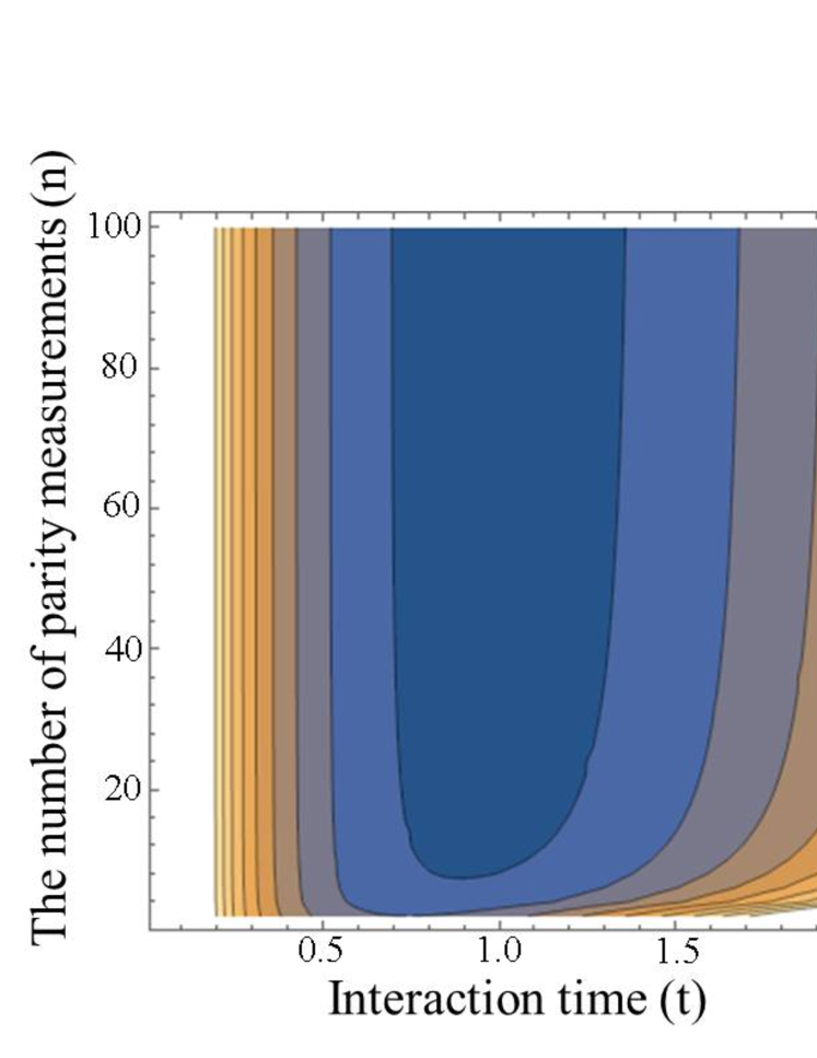
Figure 2: Uncertainty of the estimation of the magnetic fields with multiple QED cycles for $s=0.5$ and $\Gamma=1$. We use the same sequence as for the QEC except that we discard the state before the readout if we detect any errors in the parity projections. As we increase the number of the parity measurements, we can decrease the uncertainty, and the minimum uncertainty is $\delta\omega\simeq 1.65/\sqrt{T\Gamma}$, which beats the one in the single-qubit sensors.

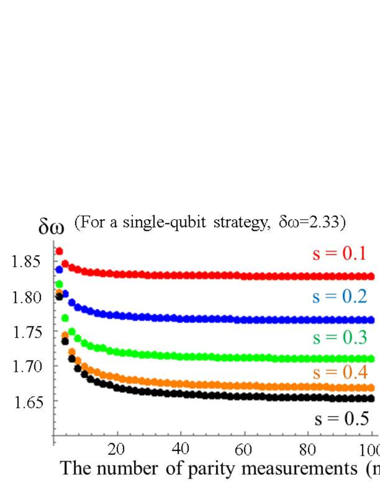
Figure 3: Uncertainty of the estimation of the magnetic fields with multiple QED cycles against the number of the parity measurements $n$. Here, we choose the interaction time $t$ to minimize the uncertainty, and we fix $\Gamma=1$.

We consider a case $s=\frac{1}{2}$ where we can get an analytical solution for the uncertainty of the estimation. Also, for simplicity, we assume $n$ is an even number. The state before the readout is calculated as

$$\rho^{(\rm{MQED})}_{n}(t)=e^{-iHt}\Big{(}\big{(}\sum_{m=0}^{\frac{n}{2}}{}_{n}C_{2m}(p_{1})^{n-2m}(1-p_{1})^{2m}\big{)}\rho_{0}$$

$$+\big{(}\sum_{m=1}^{\frac{n}{2}}{}_{n}C_{2m-1}(p_{1})^{n-2m+1}(1-p_{1})^{2m-1}\big{)}\hat{\sigma}_{z}^{(1)}\rho_{0}\hat{\sigma}_{z}^{(1)}\Big{)}e^{iHt}$$

where $p_{1}=\frac{\frac{1}{4}(1+2e^{-\Gamma\tau}+e^{-2\Gamma\tau})}{(\frac{1+e^{-2\Gamma\tau}}{2})}$ and ${}_{n}C_{m}=\frac{n!}{(n-m)!m!}$. We obtain this state with a success probability of $(\frac{1+e^{-2\Gamma\tau}}{2})^{n}$. We consider the following probability.

$$P^{(\rm{MQED})}_{+1}={\rm{Tr}}[|+^{(y)}_{\rm{L}}\rangle\langle+^{(y)}_{\rm{L}}|\rho^{(\rm{MQED})}_{n}(t)]\ \ \$$

$$=\Big{(}\sum_{m=0}^{\frac{n}{2}}{}_{n}C_{2m}(p_{1})^{n-2m}(1-p_{1})^{2m}\Big{)}\frac{1+\sin\omega t}{2}$$

$$+\Big{(}\sum_{m=1}^{\frac{n}{2}}{}_{n}C_{2m-1}(p_{1})^{n-2m+1}(1-p_{1})^{2m-1}\Big{)}\frac{1-\sin\omega t}{2}$$

where $|+^{(y)}_{\rm{L}}\rangle=\frac{1}{\sqrt{2}}(|00\rangle+i|11\rangle)$. The sensitivity is given as

$$\delta\omega = \frac{\sqrt{P^{(\rm{MQED})}_{+1}(1-P^{(\rm{MQED})}_{+1})}}{|\frac{dP^{(\rm{MQED})}_{+1}}{d\omega}|}\cdot\frac{1}{\sqrt{\frac{T}{t}(\frac{1+e^{-2\Gamma\frac{t}{n}}}{2})^{n}}}$$ (16)

$$\simeq 1.65/\sqrt{T\Gamma}$$

where we choose $t$ and $n$ to minimize $\delta\omega$. We plot the $\delta\omega$ to show the dependence of $t$ and $n$ in the Fig. 2. As we increase the number of the parity measurements, the uncertainty increases and converges to the value described in the Eq. (16).

We also perform numerical simulations to calculate the uncertainty of the estimation in the QED strategy for other values of $s$. The results are plotted in the Fig. 3. We confirmed that the QED strategy actually beats the single-qubit sensors for the other values of $s$.

We discuss an intuitive reason why multiple QED strategy can beat the single QED strategy. If we perform a single parity measurement in the end of the time evolution, there will be a possibility that bit flip errors occur twice within the time evolution, which induces undetected error. Multiple QED provides us with a capability to eliminate such a possibility so that we can significantly suppress the effect of the bit flip error.

III.3 Adaptive feedback

Interestingly, we can further improve the sensitivity by using an adaptive feedback. In the last subsection, we discussed multiple QED rounds where we use the same sequence as QEC except that we discard the state before the readout if we detect any errors in the parity projections. However, this strategy is inefficient, because we waste time between the parity measurement and the readout once we have detected an error. For example, when we detect the error at $k$-th parity measurements, we have a time $\frac{n-k}{n}t$ before the readout, and we spend this time without contributing to the sensitivity. To improve this point, we propose to use an adaptive feedback where we immediately initialize the state for the next round whenever we detect the error, as shown in the Fig. 4.

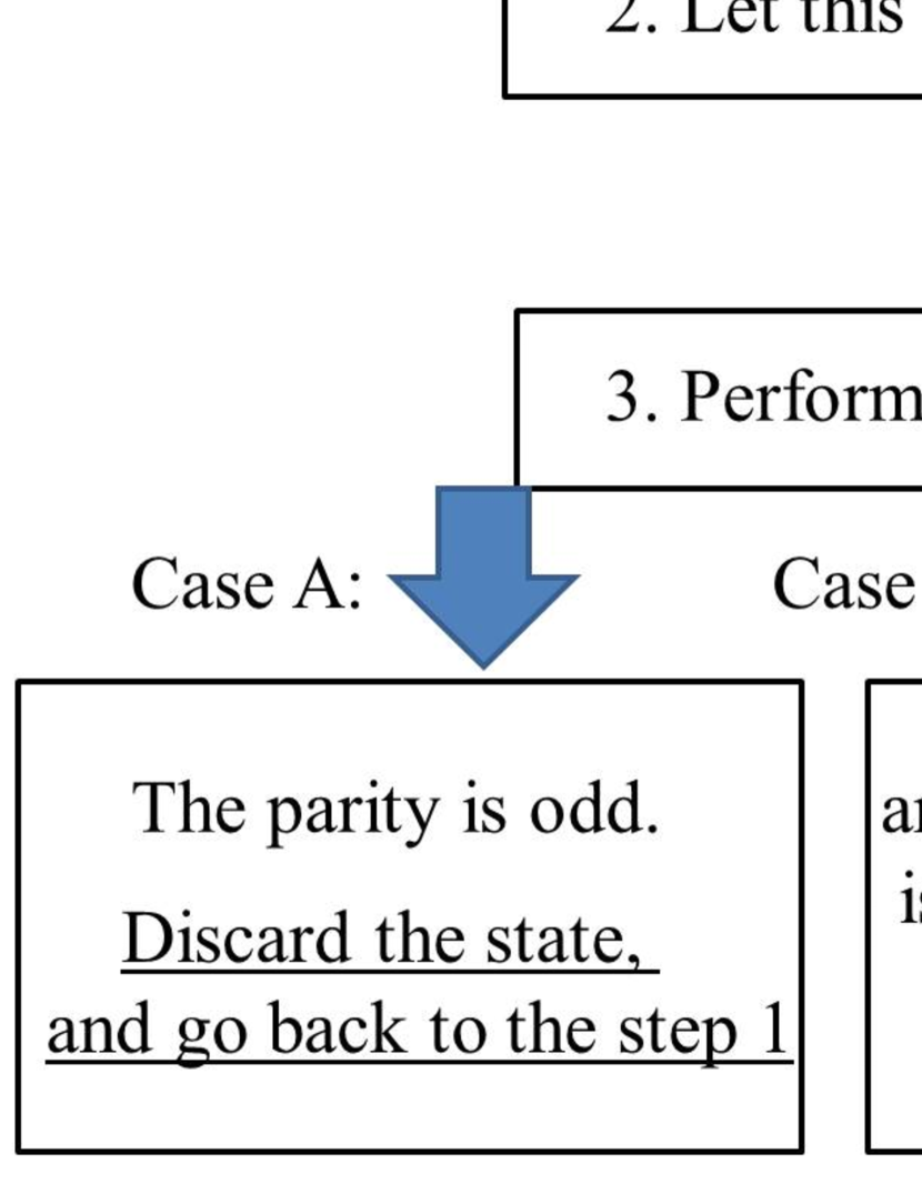
Figure 4: The schematic to perform an adaptive feedback in our QED strategy to estimate the target magnetic fields. Depending on the measurement results, we will implement different operations.

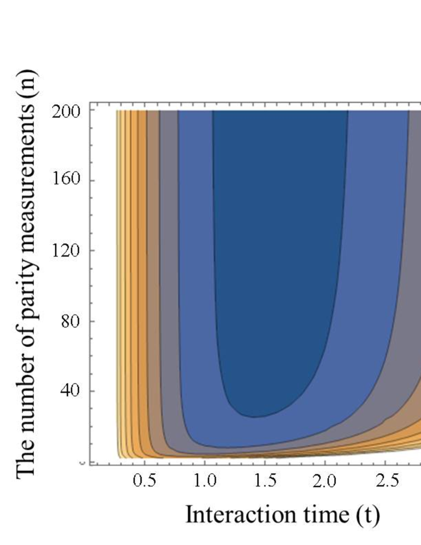
Figure 5: Uncertainty of the estimation of the magnetic fields with adaptive feedback for $s=0.5$ and $\Gamma=1$. The detail of the procedure is given in the Fig. 4. As we increase the number of the parity measurements, we can decrease the uncertainty, and the minimum uncertainty is $\delta\omega\simeq 1.25/\sqrt{T\Gamma}$, which is better than the QED strategy without adaptive feedback.

Firstly, we consider a case for $s=0.5$ to obtain an analytical solution. In this adaptive feedback strategy, we can calculate the average time for a single cycle of the sensing as follows. If we detect the error in the $k$ the parity measurements, the time between the state preparation and the last parity projection is $\frac{k}{n}t$. This event occurs with a probability of $(p_{s})^{k-1}(1-p_{s})$ where $p_{s}=\frac{1+e^{-2\Gamma\tau}}{2}$ denotes a probability that we do not detect the error. On the other hand, if we do not detect any errors for $n$ parity measurements (which occurs with a probability of $(p_{s})^{n}$), the time between the state preparation and the final readout is $t$. So the average time for a single cycle of this adaptive feedback strategy is

$$t_{\rm{av}}=(p_{s})^{n}t+\sum_{k=1}^{n}(p_{s})^{k-1}(1-p_{s})k\frac{t}{n}.$$ (17)

We can calculate the number of the readout measurements for a given time $T$ as $N=\frac{T}{t_{\rm{av}}}(\frac{1+e^{-2\Gamma\frac{t}{n}}}{2})^{n}$. The sensitivity is given as

$$\delta\omega = \frac{\sqrt{P^{(\rm{MQED})}_{+1}(1-P^{(\rm{MQED})}_{+1})}}{|\frac{dP^{(\rm{MQED})}_{+1}}{d\omega}|}\cdot\frac{1}{\sqrt{\frac{T}{t_{\rm{av}}}(\frac{1+e^{-2\Gamma\frac{t}{n}}}{2})^{n}}}$$ (18)

$$\simeq 1.25/\sqrt{T\Gamma}$$

where we choose $t$ and $n$ to minimize $\delta\omega$. We plot the $\delta\omega$ to show the dependence of $t$ and $n$ in the Fig. 5. Again, as we increase the number of the parity measurements, the uncertainty increases and converges to the value of the Eq. (18).

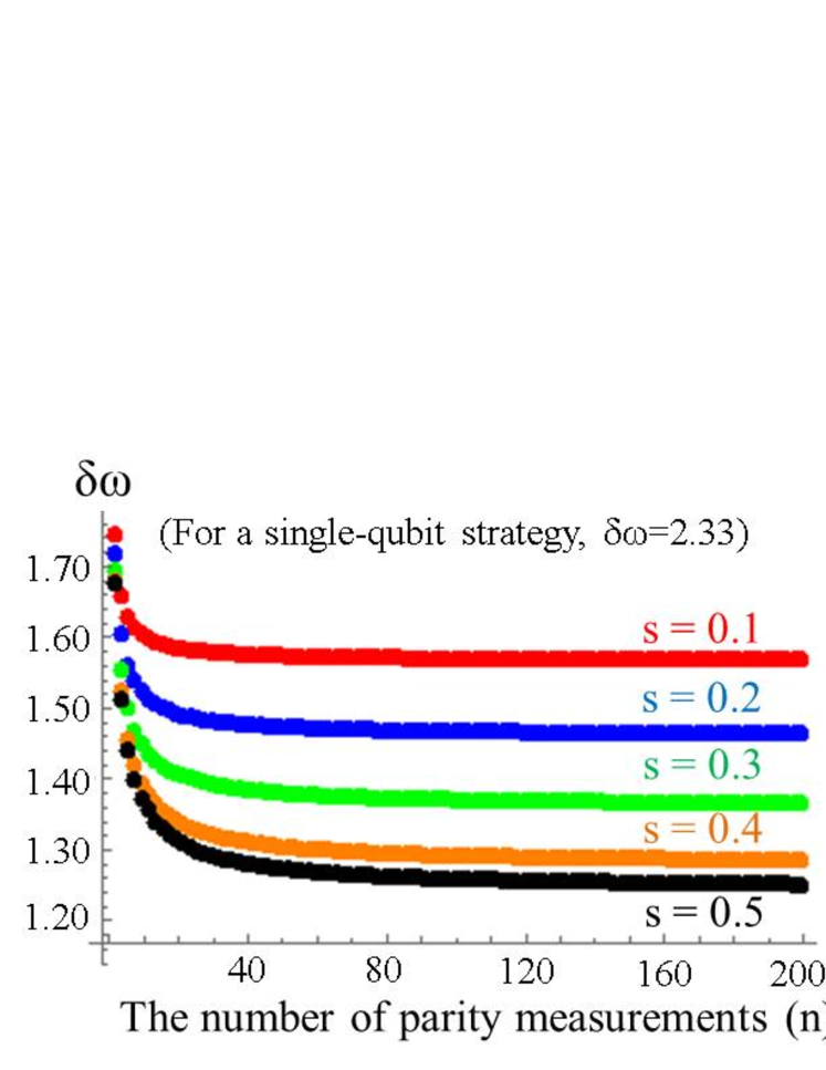
Figure 6: Uncertainty of the estimation of the magnetic fields with adaptive feedback against the number of the parity measurements $n$. Here, we choose the interaction time $t$ to minimize the uncertainty, and we fix $\Gamma=1$.

We also performed numerical simulations to calculate the uncertainty of the estimation in the adaptive feedback strategy for other values of $s$. The results are plotted in Fig. 6. We confirmed that the adaptive strategy improves the sensitivity over the non-adaptive strategy.

III.4 Imperfect parity projection

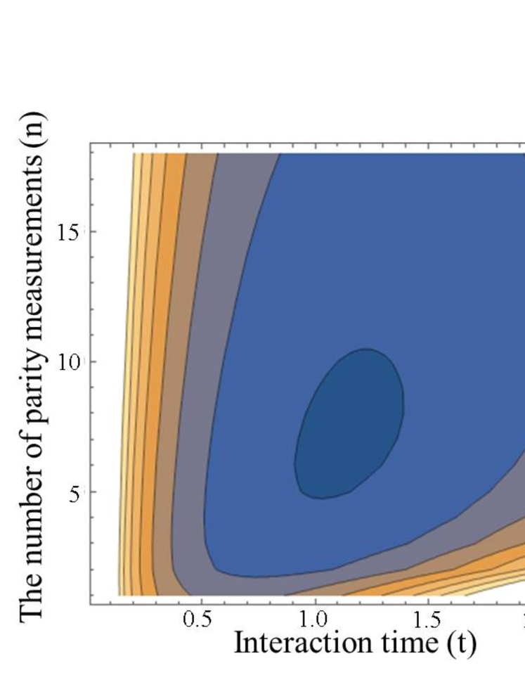
Figure 7: Uncertainty of the estimation of the magnetic fields by using imperfect parity projections with a finite error rate of $\epsilon$. Here, we fix $s=0.5$, $\epsilon=0.02$, and $\Gamma=1$. There exist an optimal set of the interaction time and the number of measurements.

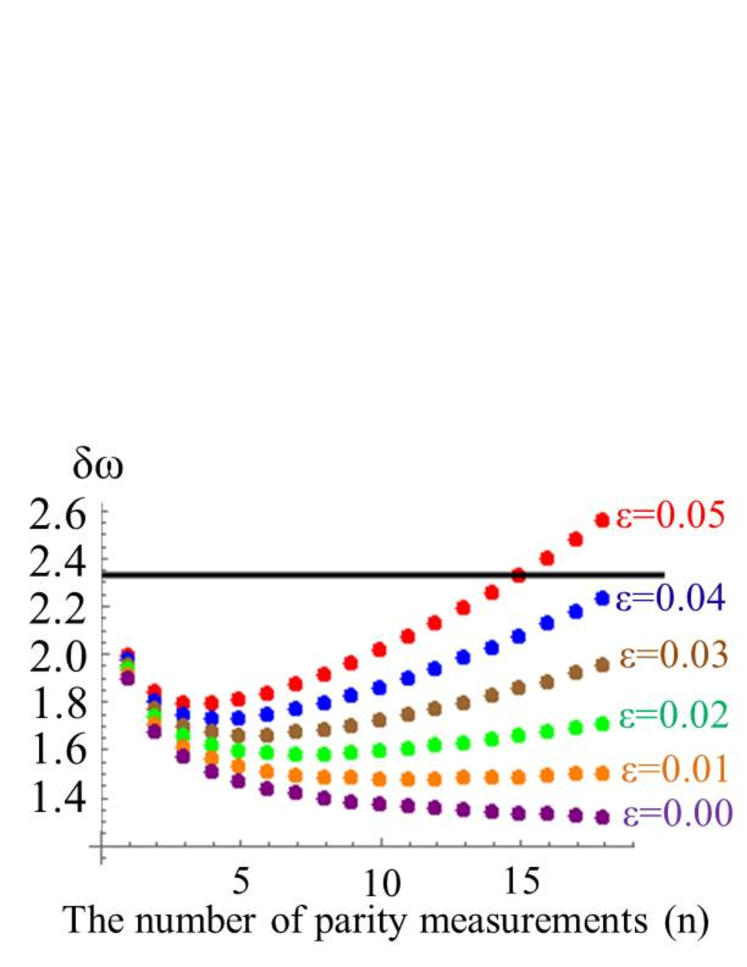
Figure 8: Uncertainty of the estimation of the magnetic fields by using imperfect parity projections with a finite error rate of $\epsilon$. Here, we choose the interaction time $t$ to minimize the uncertainty, and we fix $s=0.5$ and $\Gamma=1$. The solid line denotes the case of the single-qubit sensors. By using the imperfect parity measurement with an error rate of $\epsilon$, our QED strategy with adaptive feedback can beat single-qubit sensors.

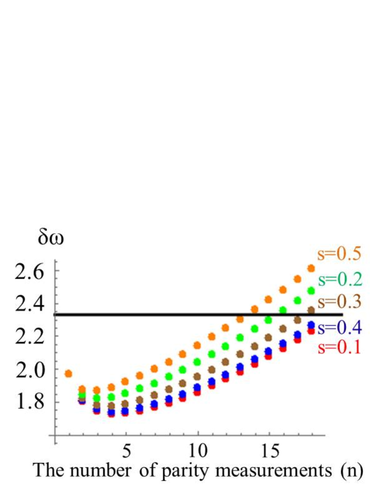
Figure 9: Uncertainty of the estimation of the magnetic fields by using imperfect parity projections with a finite error rate of $\epsilon$. Here, we choose the interaction time $t$ to minimize the uncertainty, and we fix $\epsilon=0.04$ and $\Gamma=1$. The solid line denotes the case of single-qubit sensors.

Finally we consider an effect of imperfect parity projections. In the QED strategy, as we increase the number of the parity projections, the uncertainty of the estimation decreases, if we assume ideal parity projections. In the actual experiments, we cannot avoid the possibility of an error in the parity measurement, and thus the optimal number of parity measurements will be a finite. We consider a model that depolarized noise occurs with a probability of $\epsilon$. If the measurement result is even, we obtain

$$\rho^{\prime}=(1-\epsilon)\frac{\hat{\mathcal{P}}_{\rm{even}}.\rho.\hat{\mathcal{P}}_{\rm{even}}}{{\rm{Tr}}[\hat{\mathcal{P}}_{\rm{even}}.\rho\hat{\mathcal{P}}_{\rm{even}}]}+\epsilon\frac{1}{4}\hat{\openone}_{\rm{pm}}$$ (19)

where the state becomes a completely mixed state with a probability of $\epsilon$. With this noise model, we numerically evaluate the performance of the adaptive feedback strategy with imperfect parity measurements. As the Figs 7, 8, and 9 show, we can beat the single-qubit sensors as long as the error rate $\epsilon$ is around four percent.

We discuss a possible reason why the large error of around four percent can be tolerated in our scheme. If depolarising noise occurs on a qubit, this can be interpreted as a random applications of Pauli matrices $\hat{\openone}$, $\hat{\sigma}_{x}$, $\hat{\sigma}_{y}$, and $\hat{\sigma}_{z}$ with equally probability. However, the parity measurement in the next round can eliminate the degrading effect of $\hat{\sigma}_{x}$ and $\hat{\sigma}_{y}$. So only one of the three noise operators can fully impact the sensitivity of our scheme.

IV Conclusion

In conclusion, we have investigated the performance of quantum error correction to improve quantum field sensing under the effect of dephasing. We have shown that the standard quantum error correction, including error detection and recovery operations, does not improve the sensitivity over the single-qubit sensors. However, we have found that, if we adopt a postselection to discard the state whenever an error is detected, we can actually achieve significant quantum enhancement, even when the operations we use are imperfect. Since energy relaxation is one of the typical noise types in solid state systems, our results pave a way to realize a quantum enhanced sensors in realistic conditions.

This work was supported by JSPS KAKENHI Grants 15K17732. Also, this work was partly supported by MEXT KAKENHI Grant Number 15H05870.

References

- Simon (1999) J. Simon, Advances in Physics 48, 449 (1999).
- Chang et al. (1992) A. Chang, H. Hallen, L. Harriott, H. Hess, H. Kao, J. Kwo, R. Miller, R. Wolfe, J. Van der Ziel, and T. Chang, Applied physics letters 61, 1974 (1992).
- Poggio and Degen (2010) M. Poggio and C. Degen, Nanotechnology 21, 342001 (2010).
- Budker and Romalis (2007) D. Budker and M. Romalis, Nature Physics 3, 227 (2007).
- Maze et al. (2008) J. Maze, P. Stanwix, J. Hodges, S. Hong, J. Taylor, P. Cappellaro, L. Jiang, M. Dutt, E. Togan, A. Zibrov, et al., Nature 455, 644 (2008), ISSN 0028-0836.
- Taylor et al. (2008) J. Taylor, P. Cappellaro, L. Childress, L. Jiang, D. Budker, P. Hemmer, A. Yacoby, R. Walsworth, and M. Lukin, Nature Physics 4, 810 (2008).
- Balasubramanian et al. (2008) G. Balasubramanian, I. Chan, R. Kolesov, M. Al-Hmoud, J. Tisler, C. Shin, C. Kim, A. Wojcik, P. Hemmer, A. Krueger, et al., Nature 455, 648 (2008).
- Huelga et al. (1997) S. Huelga, C. Macchiavello, T. Pellizzari, A. Ekert, M. Plenio, and J. Cirac, Phys. Rev. Lett. 79, 3865 (1997).
- Degen et al. (2016) C. Degen, F. Reinhard, and P. Cappellaro, arXiv preprint arXiv:1611.02427 (2016).
- Kessler et al. (2014) E. M. Kessler, I. Lovchinsky, A. O. Sushkov, and M. D. Lukin, Phys. Rev. Lett. 112, 150802 (2014).
- Arrad et al. (2014) G. Arrad, Y. Vinkler, D. Aharonov, and A. Retzker, Phys. Rev. Lett. 112, 150801 (2014).
- Dür et al. (2014) W. Dür, M. Skotiniotis, F. Froewis, and B. Kraus, Phys. Rev. Lett. 112, 080801 (2014).
- Herrera-Martí et al. (2015) D. A. Herrera-Martí, T. Gefen, D. Aharonov, N. Katz, and A. Retzker, Phys. Rev. Lett. 115, 200501 (2015).
- Gottesman (2009) D. Gottesman, Quantum Information Science and Its Contributions to Mathematics 68, 13 (2009).
- Gladchenko et al. (2009) S. Gladchenko, D. Olaya, E. Dupont-Ferrier, B. Doucot, L. B. Ioffe, and M. E. Gershenson, Nature Physics 5, 48 (2009).
- Reed et al. (2012) M. Reed, L. DiCarlo, S. Nigg, L. Sun, L. Frunzio, S. Girvin, and R. Schoelkopf, Nature 482, 382 (2012).
- Córcoles et al. (2015) A. Córcoles, E. Magesan, S. J. Srinivasan, A. W. Cross, M. Steffen, J. M. Gambetta, and J. M. Chow, Nature communications 6 (2015).
- Kelly et al. (2015) J. Kelly, R. Barends, A. Fowler, A. Megrant, E. Jeffrey, T. White, D. Sank, J. Mutus, B. Campbell, Y. Chen, et al., Nature 519, 66 (2015).
- Waldherr et al. (2014) G. Waldherr, Y. Wang, S. Zaiser, M. Jamali, T. Schulte-Herbrüggen, H. Abe, T. Ohshima, J. Isoya, J. Du, P. Neumann, et al., Nature 506, 204 (2014).
- Nigg et al. (2014) D. Nigg, M. Mueller, E. A. Martinez, P. Schindler, M. Hennrich, T. Monz, M. A. Martin-Delgado, and R. Blatt, Science 345, 302 (2014).
- Unden et al. (2016) T. Unden, P. Balasubramanian, D. Louzon, Y. Vinkler, M. B. Plenio, M. Markham, D. Twitchen, A. Stacey, I. Lovchinsky, A. O. Sushkov, et al., Phys. Rev. Lett. 116, 230502 (2016).
- Cohen et al. (2016) L. Cohen, Y. Pilnyak, D. Istrati, A. Retzker, and H. Eisenberg, Phys. Rev. A 94, 012324 (2016).
- Slichter (2013) C. P. Slichter, Principles of magnetic resonance, vol. 1 (Springer Science & Business Media, 2013).
- Viola et al. (1999) L. Viola, E. Knill, and S. Lloyd, Physical Review Letters 82, 2417 (1999).
- Bylander et al. (2011) J. Bylander, S. Gustavsson, F. Yan, F. Yoshihara, K. Harrabi, G. Fitch, D. G. Cory, Y. Nakamura, J. S. Tsai, and W. D. Oliver, Nature Physics 7, 565 (2011).
- Yan et al. (2015) F. Yan, S. Gustavsson, A. Kamal, J. Birenbaum, A. Sears, D. Hover, T. Gudmundsen, J. Yoder, T. Orlando, J. Clarke, et al., arXiv preprint arXiv:1508.06299 (2015).
- Lindblad (1976) G. Lindblad, Communications in Mathematical Physics 48, 119 (1976).
- Hornberger (2009) K. Hornberger, in Entanglement and Decoherence (Springer, 2009), pp. 221–276.
- Gardiner and Zoller (2004) C. W. Gardiner and P. Zoller, Quantum Noise (Springer, Berlin, 2004).
- Hein et al. (2005) M. Hein, W. Dür, and H.-J. Briegel, Physical Review A 71, 032350 (2005).