SeDMiD for Confusion Detection: Uncovering Mind State from Time Series Brain Wave Data

Abstract

Understanding how brain functions has been an intriguing topic for years. With the recent progress on collecting massive data and developing advanced technology, people have become interested in addressing the challenge of decoding brain wave data into meaningful mind states, with many machine learning models and algorithms being revisited and developed, especially the ones that handle time series data because of the nature of brain waves. However, many of these time series models, like HMM with hidden state in discrete space or State Space Model with hidden state in continuous space, only work with one source of data and cannot handle different sources of information simultaneously. In this paper, we propose an extension of State Space Model to work with different sources of information together with its learning and inference algorithms. We apply this model to decode the mind state of students during lectures based on their brain waves and reach a significant better results compared to traditional methods.

1 Introduction

Understanding how human brain functions has been an attractive research question in recent years Mitchell et al. (2008). One important progress is on collecting a large amount of brain wave data with different technologies, like fMRI Wehbe et al. (2014), MEG Sudre et al. (2012) and EEG Wang et al. (2013). The nature of these data collecting technologies have introduced a variety of substantial challenges in understanding these data with machine learning techniques. For example, MEG and EEG technologies can describe the brain with considerable temporal granularity, but with a relatively low spatial resolution. Therefore, machine learning techniques that can handle temporal dependencies are highly appreciated.

Fortunately, in recent years, there is an increasing trend towards the use models to work with time series problem. For example, Khaleghi and Ryabko (2013) find the points in time where the probability distribution generating the data has changed given a heterogeneous time-series sample. Anava et al. (2013) use regret minimization techniques to develop effective online learning algorithms for predicting a time series using autoregressive moving average model. Alon et al. (2003) fit a finite mixture of HMMs in motion data, using the expectation maximization (EM) framework, aiming at discovering groupings of similar object motions that were observed in a video collection. Also, Hidden Markov Models or other graph-based methods are often used for the purpose like speech recognition, pattern recognition and neural networks, similar to Nahar et al. (2016), Schwenk (1999), Bar-Joseph (2004) and LeCun and Bengio (1995). In a more rigorous setting, a lot more theoretical questions are being asked and solved for time series machine learning these days. For example, Khaleghi and Ryabko (2013, 2014) derive theories for estimation of highly dependent time series data. Kuznetsov and Mohri (2014, 2015) push the theoretical work further for non-stationary time series problems. Rakhlin and Sridharan (2013); anava2013onlinekuznetsov2016time naturally combines the problem of analyzing time series data with online learning, which opens the door to a whole area of new problems.

With the guidance of previous work on time series data. In this paper, we present Sequence Data based Mind-Detecting (SeDMiD) Model , a novel time series method to uncover the state of brain using more than a typical source of EEG/MEG recordxings. Others sources like video recordings or audio data can be supplemented for better performance on brain state estimation.

We also develop the learning algorithm for SeDMiD based on sparsity regularized linear system, and the inference algorithm as an extension of Viterbi algorithm under Gaussian assumption for continuous space. The results show that, the performance of SeDMiD can uncover the mind state based on brain waves with a significant better results than traditional methods.

Our contribution of this paper is three-fold:

• We propose a SeDMiD that can analyze time series brain wave data with extra sources of information.

• We improve the existing vertibi algorithm to enable the inference of SeDMiD model.

• We show the possibility of deciphering students’ mind state of understanding lectures with brain wave data.

The rest of this paper is organized as following. Section 2 describes some work that others did to solve the prediction problem using MEG data. Section 3 raises the novel model and describe its learning and inference method, while section 4 shows the result of our experiment. Finally, Section 5 concludes and suggests future work.

2 Related Work

There are many works implementing time series technology to deal with the problem about MEG/EEG data. It is worth noting that both electroencephalography (EEG) and magnetoencephalography (MEG) provide a more direct measure of the electrical activity in the brain, as is described professionally in the work of Michel (2009) and Proudfoot et al. (2014). He et al. (2008) measure the difference in electric potentials on the scalp and captures high frequency oscillations on the millisecond timescale that is most relevant for the characterisation of cognitive processes. There are many existing work to do experiments and discover new knowledge in several fields. Moghadamfalahi et al. (2015) use abstract—noninvasive EEG-based brain–computer interfaces (BCI) for intent detection, specifically for EEG-based BCI typing systems. Phillips et al. (1997) have developed a Bayesian framework for image estimation from combined MEG/EEG data.

EEG signal is a kind of voltage signal that can be measured on the surface of the scalp, arising from large areas of coordinated neural activity manifested as synchronization (groups of neurons firing at the same rate), described by Niedermeyer and da Silva (2005). This neural activity varies as a function of development, mental state, and cognitive activity, and the EEG signal can measurably detect such variation Marosi et al. (2002), Lutsyuk et al. (2006), Berka et al. (2007), Wang et al. (2013) which in turn are important for and predictive of learning Baker et al. (2010).

On the other hand, hidden Markov model is also widely implemented to make best use of MEG/EEG recordings. Rukat et al. (2016) analyses the temporal and spatial dynamics of physiological substrate of cognitive processes as measured by EEG, with a hidden Markov model. Liu et al. (2010) combine kernel principal component analysis (KPCA) and HMM to differentiate mental fatigue states with the help of EEG data. Ko and Sim (2011) describe a procedure of classification of motor imagery EEG signals using HMM, which can tell the person is performing left, right hand or foots motor imagery based on the current EEG recordings. What is more, another bio-signal named electrocardiogram (ECG) is also suitable for Markov model. Coast et al. (1990) and Andreão et al. (2006) describe a new approach to ECG arrhythmia analysis based on HMM. Inspired by these work, we propose a novel model to analyze time series brain wave data with extra sources of information.

3 SeDMiD Model and Its Learning and Inference Algorithm

We propose a novel state-space model for inferring people’s state using several sources of information simultaneously including MEG/EEG recordings, named Sequence Data based Mind-Detecting (SeDMiD) Model. In this section, we will first introduce the model, and then show its learning and inference algorithm respectively.

3.1 SeDMiD

The aim of our work is to raise a model for brain-state estimation using MEG/EEG recordings while considering other essential time-series sources at the same time. A pictorial representation of our model can be found in Figure 1. Notations of this paper is illustrated in the caption of Figure 1.

In the SeDMiD model, we firstly assume that the extra time-series sources can match exactly with brain wave signals in aspect of time stamps, which means $\vec{S_{i}}$, $\vec{C_{i}}$ and $\vec{M_{i}}$ are sampled at the same time. And we simplify the mind state inferring task as a binary decision of states $\vec{C_{i}}$, indicating that people is either happy or sad, or students are either confused or not. We also assume that MEG/EEG recordings $\vec{M_{i}}$ have linear dependence on current external source and current mind state, since brain signal is easily affected by people’s internal mind situation and outside influence on them Baker et al. (2010). Additionally, current mind state $\vec{M_{i}}$ depends linearly on previous status and current video contents, because brain state often has a close connection with its state few seconds ago, and other sources like videos also affect the mind state. Finally, the complementary source is a continuous time-series process, thus current recording is dependent on the former one, and to simplify the model, we assume linear dependency again.

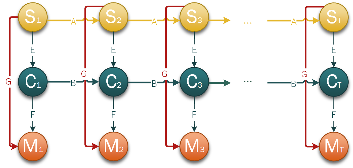
Figure 1: The proposed model. For the time-stamp at $i$, $\vec{M_{i}}$ corresponds to EEG/MEG recording and $\vec{C_{i}}$ corresponds to mind states (e.g. happy/sad, confused/non-confused). $\vec{S_{i}}$ is extra source information (e.g. video/audio data). $\vec{A}$, $\vec{B}$, $\vec{E}$, $\vec{F}$ and $\vec{G}$ are stationary transition matrices that describe the dynamics among states in the graph.

Further, we assume that the supplemental source data $\{\vec{S_{i}}\}_{i=1}^{n}$ can be described by Gaussian distribution.

$$\vec{S_{1}}\thicksim\mathcal{N}(\vec{\mu_{s}},\vec{\sigma_{s}})\\$$

$$\vec{S_{i}}\thicksim\mathcal{N}(\vec{A}\cdot\vec{S_{i-1}},~{}\vec{\Lambda_{i}})$$

We also assume that mind states $\{\vec{C_{i}}\}_{i=1}^{n}$ is in form of Gaussian distribution.

$$\vec{C_{1}}\thicksim\mathcal{N}(\vec{\mu_{c}},\vec{\sigma_{c}})$$

$$\vec{C_{i}}\thicksim\mathcal{N}\left\lgroup\bm{l(}\vec{E}\cdot\vec{S_{i}}+\vec{B}\cdot\vec{C_{i-1}}\bm{)},~{}\vec{\Omega_{i}}\right\rgroup$$

Considering the assumption that only on-and-off state exist in space $\set{C}$, we use the function $\bm{l()}$ to map the score of positive state ($\vec{E}\cdot\vec{S_{i}}+\vec{B}\cdot\vec{C_{i-1}}$) into two dimensions above.

$$\bm{l(}x\bm{)}=\begin{bmatrix}\frac{1}{1+e^{x}}\\ \frac{e^{x}}{1+e^{x}}\end{bmatrix}$$

Thus brain wave recordings $\{\vec{M_{i}}\}_{i=1}^{n}$ also follows Gaussian distribution because it is the linear combination of $\{\vec{S_{i}}\}_{i=1}^{n}$ and $\{\vec{C_{i}}\}_{i=1}^{n}$, as the mean of $\vec{M_{i}}$ is $\vec{G}\cdot\vec{S_{i}}+\vec{F}\cdot\vec{C_{i}}$ and co-variance is $\vec{\Sigma_{i}}$.

$$\vec{M_{i}}\thicksim\mathcal{N}(\vec{G}\cdot\vec{S_{i}}+\vec{F}\cdot\vec{C_{i}},~{}\vec{\Sigma_{i}})$$

The practical meaning of notations in the model is described by Table 1.

MEG Feature Notation Description $\vec{S_{i}}$ Features of supplemental source information at time $i$ $\vec{C_{i}}$ Mind States at time $i$ $\vec{M_{i}}$ Brain wave signal recordings (EEG/MEG) at time $i$ $\vec{A}$ Linear Relationship between adjacent supplemental source information $\vec{B}$ Linear Relationship between adjacent mind states $\vec{E}$ Linear Relationship between supplemental source and mind state $\vec{F}$ Linear Relationship between mind state and brain wave signal $\vec{G}$ Linear Relationship between supplemental source and brain wave signal

Table 1: Practical Meaning of Notations in SeDMid model

3.2 Learning

Here we introduce the parameter learning algorithm of $\vec{A}$, $\vec{B}$, $\vec{E}$, $\vec{F}$and $\vec{G}$ for SeDMiD. Because of the nature of the task, a supervised training training procedure, with $\vec{S}$, $\vec{C}$, $\vec{M}$ known, is sufficient. At training, at time-stamp $i$, we can observe MEG/EEG recording $\vec{M_{i}}$, supplemental source data $\vec{S_{i}}$ and current mind state $\vec{C_{i}}$. Thus, parameter learning is a maximum likelihood estimation (MLE) problem, in which case linear regression is the solution. However, supplemental source data generally comes with a higher dimension than response variable space. Therefore, sparsity regularize is required for transition matrix $\vec{S}$ by eq:learning_A in a sparse form.

$$\vec{M_{i}}=\begin{bmatrix}\vec{G}&\vec{F}\end{bmatrix}\begin{bmatrix}\vec{S_{i}}\\ \vec{C_{i}}\end{bmatrix}$$ (1)

$$\vec{C_{i}}=\begin{bmatrix}\vec{B}&\vec{E}\end{bmatrix}\begin{bmatrix}\vec{C_{i}}\\ \vec{S_{i+1}}\end{bmatrix}$$ (2)

$$\vec{S_{i+1}}=\vec{A}\cdot\vec{S_{i}}$$ (3)

3.3 Inference

In inference, observation only contains brain wave recordings, so we want to estimate mind state $\vec{C_{i}}$ and even further inference complementary data $\vec{S_{i}}$. With the observation $\vec{M_{i}}$ and five transition matrices that learned in the learning phase, we formulate an inference method to find the best sequence of mind states $\vec{C_{1}},\vec{C_{2}},\dots,\vec{C_{T}}$ and features of complementary data $\vec{S_{1}},\vec{S_{2}},\dots,\vec{S_{T}}$. A natural choice for inference on the model is Viterbi algorithm Forney (1973). However, the problem is that the state space $\set{S}$ and $\set{M}$ are infinite, and we assume that $S_{i}$ and $M_{i}$ follow Gaussian distribution, we formulate the inference mathematically in Gaussian form. Consider the Viterbi function at the time-stamp $t$ is calculated by eq:viterbi_1, given by the factorization of graphic model shown in figure1.

$$\vec{V_{t}}(\vec{S_{t}},\vec{C_{t}})=\max_{\vec{S_{t-1}},\vec{C_{t-1}}}[P(\vec{M_{t}}|\vec{S_{t}},\vec{C_{t}})P(\vec{S_{t}}|\vec{S_{t-1}})P(\vec{C_{t}}|\vec{S_{t}},\vec{C_{t-1}})V_{t-1}(\vec{S_{t-1}},\vec{C_{t-1}})]$$ (4)

To begin with, we consider to calculate the Viterbi function $\vec{V_{1}}$ at the start point of the whole process when t = 1.

$$\begin{split}\vec{V_{1}}(\vec{S_{1}},\vec{C_{1}})&=P(\vec{M_{1}}|\vec{S_{1}},\vec{C_{1}})P(\vec{S_{1}})P(\vec{C_{1}}|\vec{S_{1}})\\ &=\mathcal{N}(\vec{G}\cdot\vec{S_{1}}+\vec{F}\cdot\vec{C_{1}},\vec{\Sigma})\cdot\mathcal{N}(\vec{\mu_{s}},\vec{\sigma_{s}})\cdot\mathcal{N}(\bm{l(}\vec{E}\cdot\vec{\mu_{s}}\bm{)},\vec{\sigma_{c}})\end{split}$$ (5)

According to the property of multiplication in Gaussian distribution, we obtain that $\vec{V_{1}}$ is also in form of Gaussian with its mean and variance shown in (6) and (7) respectively.

$$\vec{\Sigma_{V_{1}}}=\left\lgroup\begin{bmatrix}\vec{\sigma_{s}}^{-1}&\vec{0}\\ \vec{0}&\vec{\sigma_{c}}^{-1}\end{bmatrix}+\begin{bmatrix}\vec{G}^{T}\\ \vec{F}^{T}\end{bmatrix}\vec{\Sigma}^{-1}\begin{bmatrix}\vec{G}&\vec{F}\end{bmatrix}\right\rgroup^{-1}$$ (6)

$$\vec{\mu_{V_{1}}}=\vec{\Sigma_{V_{1}}}\left\lgroup\begin{bmatrix}\vec{\sigma_{s}}^{-1}\vec{\mu_{s}}\\ \vec{\sigma_{c}}^{-1}\bm{l(}\vec{E}\cdot\vec{\mu_{s}}\bm{)}\end{bmatrix}+\begin{bmatrix}\vec{G}^{T}\\ \vec{F}^{T}\end{bmatrix}\vec{\Sigma}^{-1}\vec{M_{1}}\right\rgroup$$ (7)

For now, the mean and covariance of Viterbi function for the beginning point have been calculated, and in order to know all the Viterbi function at every time-stamp, we find when $t\geqslant 2$:

$$\vec{V_{t}}(\vec{S_{t}},\vec{C_{t}})=\max_{\vec{S_{t-1}},\vec{C_{t-1}}}P(\vec{C_{t}}|\vec{S_{t}},\vec{C_{t-1}})P(\vec{S_{t}}|\vec{S_{t-1}})V_{t-1}(\vec{S_{t-1}},\vec{C_{t-1}})P(\vec{M_{t}}|\vec{S_{t}},\vec{C_{t}})$$ (8)

Also, we can calculate the mean and covariance since for time $t$, $\vec{S_{t}}$ and $\vec{C_{t}}$ are in the form of Gaussian distribution.

$$\vec{\Sigma}_{\vec{V_{2}}}=\left\lgroup\vec{\Phi^{-1}}+\begin{bmatrix}\vec{G}^{T}\\ \vec{F}^{T}\end{bmatrix}\vec{\Sigma}^{-1}\begin{bmatrix}\vec{G}&\vec{F}\end{bmatrix}\right\rgroup^{-1}$$ (9)

$$\vec{\mu}_{\vec{V_{2}}}=\vec{\Sigma}_{V_{2}}\left\lgroup\vec{\Phi^{-1}}\cdot\vec{\mu}_{\vec{V_{1}}}+\begin{bmatrix}\vec{G}^{T}\\ \vec{F}^{T}\end{bmatrix}\vec{\Sigma}^{-1}\vec{M_{2}}\right\rgroup$$ (10)

where

$$\vec{\Phi}=\left\lgroup\begin{bmatrix}\vec{\Lambda}^{-1}&\vec{0}\\ \vec{0}&\vec{\Omega}^{-1}\end{bmatrix}+\left\lgroup\begin{bmatrix}(\vec{A}^{-1})^{T}&\vec{0}\\ \vec{0}&(\vec{B}^{-1})^{T}\end{bmatrix}\vec{\Sigma}_{V_{1}}^{-1}\begin{bmatrix}\vec{A}^{-1}&\vec{0}\\ \vec{0}&\vec{B}^{-1}\end{bmatrix}\right\rgroup\right\rgroup^{-1}$$ (11)

Once the means and co-variances are calculated for all supplemental source data and mind state sequence, the best sequence of $\vec{S}$ and $\vec{C}$ can be inferred by calculating backwards. So we start the inference at the end of the time sequence.

$$\begin{bmatrix}\vec{S_{T}}\\ \vec{C_{T}}\end{bmatrix}=\arg\max_{\vec{S_{T}},\vec{C_{T}}}\mathcal{N}(\vec{\mu}_{V_{T}},\vec{\Sigma}_{V_{T}})$$ (12)

Note that the mean of the final state is calculated exactly, we proceed to infer the former state that lead to the current one, so the formula to calculate the former state based on current state is shown in (13).

$$\begin{bmatrix}\vec{S_{T-1}}\\ \vec{C_{T-1}}\end{bmatrix}=\arg\max_{\vec{S_{T-1}},\vec{C_{T-1}}}\mathcal{N}(\vec{\gamma},\vec{\tau})$$ (13)

where

$$\vec{\tau}=\left\lgroup\vec{\Sigma}_{V_{T-1}}^{-1}+\begin{bmatrix}(\vec{E}\cdot\vec{A})^{T}\\ \vec{B}^{T}\end{bmatrix}\vec{\Omega}^{-1}\begin{bmatrix}\vec{E}\cdot\vec{A}&\vec{B}\end{bmatrix}+\begin{bmatrix}\vec{A}^{T}\vec{\Lambda}^{-1}\vec{A}&\vec{0}\\ \vec{0}&\vec{0}\end{bmatrix}\right\rgroup^{-1}$$ (14)

$$\vec{\gamma}=\vec{\tau}\left\lgroup\vec{\Sigma}_{V_{T-1}}^{-1}\vec{\mu}_{V_{T-1}}+\begin{bmatrix}(\vec{E}\cdot\vec{A})^{T}\\ \vec{B}^{T}\end{bmatrix}\vec{\Omega}^{-1}\begin{bmatrix}\vec{S_{T}}\\ \vec{C_{T}}\end{bmatrix}+\begin{bmatrix}\vec{A}^{T}\vec{\Lambda}^{-1}\vec{A}&\vec{0}\\ \vec{0}&\vec{0}\end{bmatrix}\begin{bmatrix}\vec{S_{T}}\\ \vec{C_{T}}\end{bmatrix}\right\rgroup^{-1}$$ (15)

Finally, by calculate all the $\vec{S_{i}}$ and $\vec{C_{i}}$ from end to the first one, we can infer mind states for each time-stamp $t\in\{1,\dots,T\}$.

4 Experiment

To solve the problem that we raised in sec:problemDef, we need to extract features of lecture videos. Using SeDMid model that we raise in sec:method,

4.1 Experiment Setting

In our experiment, we set up a task to estimate students’ mind states in a given lecture session, finding out they are confused or not with the data from Wang et al. (2013). Every participants is asked to watch 10 lecture videos, the length of which is around 2 minutes.The two-minute period is called an ’experiment period’. In all there are 10 students participate in the experiments so there are 100 data points in total. During every experiment period, their EEG signals are recorded in the frequency of 1 Hz, and EEG signals here have 11 features, including Proprietary measure of mental focus, 1-3 Hz of power spectrum and so on. Students are asked to annotate whether they are confused or not based on every whole experiment period, and every second in the period by the annotation is noted. The beginning and the end of every experiment is cut off with consideration of reducing noise, only left the middle 112 seconds for analysis. Finally, lecture videos are served as supplemental source data.

4.2 Video Feature Extraction

We use the tool kit OpenCV developed by Bradski and Kaehler (2008) to extract video features like optical features and object movement information, and openSMILE developed by Eyben et al. (2010) to extract features in audio data, such as lecturer’s speech speed and intonation. As a result, we obtain video image features with 1440 dimensions while audio features have 6669 dimensions, thus we get 8109 dimensions for video features in total. Since both MEG recordings and students’ status vector is collected in the frequency of 1 Hz, we sample the feature vector every 1 second in order to alignment the data for SeDMiD model.

4.3 Performance Comparison

We use the simple state space model (SSM) as baseline, which only make use of EEG data, and current mind state only depends on the former state, while current EEG recording depends on current mind state. SSM does not make use of video features. We also compare our model with logistic regression, which employ brain wave signals without other sources. As is shown in the ROC curve in Figure 2, we find that our SedMid model outperform the simple HMM model and logistic regression, with the accuracy of ours reaches 87.76% while simple HMM only gets 53% and logistic regression 60%. In the experiment, We find that errors that SeDMiD makes always exist at the beginning of experiment period, and it will lead to correct result in few time. It is intuitive that SeDMiD model often makes mistakes at beginning of every experiment period because it can perform better with more data gets concluded.

Figure 2: The ROC curve for comparing the performance of SeDMiD model, Simple State Model (SSM) and logistic regression. SeDMiD greatly outperforms the others.

5 Conclusion

In this work, we propose an novel state space model called Sequence Data based Mind-Detecting (SeDMiD) Model, which analyzes time series brain wave data with extra sources of information, improving the existing vertibi algorithm to enable the inference. We evaluate the effectiveness of SeDMiD model by comparing with simple Markov model and logistic regression. The performance of our model has a 30% higher in accuracy than the normal one.

Apart from proposing the SeDMiD model, our contribution includes showing the possibility of deciphering students’ mind state of understanding lectures with brain wave data. This work is also useful in real world implementation, since teachers can modify their teaching strategy based on audiences’ status if it can be inferred.

This work was supported by International School, Beijing University of Posts and Telecommunications. We thank Hao Ding for advising the method of extracting videos’ features and dormitory administrator in Student Building 5, BUPT, for providing electronic power for running experiment at night.

References

- Alon et al. (2003) Jonathan Alon, Stan Sclaroff, George Kollios, and Vladimir Pavlovic. Discovering clusters in motion time-series data. In Computer Vision and Pattern Recognition, 2003. Proceedings. 2003 IEEE Computer Society Conference on, volume 1, pages I–375. IEEE, 2003.
- Anava et al. (2013) Oren Anava, Elad Hazan, Shie Mannor, and Ohad Shamir. Online learning for time series prediction. In COLT, pages 172–184, 2013.
- Andreão et al. (2006) Rodrigo Varejão Andreão, Bernadette Dorizzi, and Jérôme Boudy. Ecg signal analysis through hidden markov models. IEEE Transactions on Biomedical engineering, 53(8):1541–1549, 2006.
- Baker et al. (2010) Ryan SJd Baker, Sidney K D’Mello, Ma Mercedes T Rodrigo, and Arthur C Graesser. Better to be frustrated than bored: The incidence, persistence, and impact of learners’ cognitive–affective states during interactions with three different computer-based learning environments. International Journal of Human-Computer Studies, 68(4):223–241, 2010.
- Bar-Joseph (2004) Ziv Bar-Joseph. Analyzing time series gene expression data. Bioinformatics, 20(16):2493–2503, 2004.
- Berka et al. (2007) Chris Berka, Daniel J Levendowski, Michelle N Lumicao, Alan Yau, Gene Davis, Vladimir T Zivkovic, Richard E Olmstead, Patrice D Tremoulet, and Patrick L Craven. Eeg correlates of task engagement and mental workload in vigilance, learning, and memory tasks. Aviation, space, and environmental medicine, 78(Supplement 1):B231–B244, 2007.
- Bradski and Kaehler (2008) Gary Bradski and Adrian Kaehler. Learning OpenCV: Computer vision with the OpenCV library. ” O’Reilly Media, Inc.”, 2008.
- Coast et al. (1990) Douglas A Coast, Richard M Stern, Gerald G Cano, and Stanley A Briller. An approach to cardiac arrhythmia analysis using hidden markov models. IEEE Transactions on biomedical Engineering, 37(9):826–836, 1990.
- Eyben et al. (2010) Florian Eyben, Martin Wöllmer, and Björn Schuller. Opensmile: the munich versatile and fast open-source audio feature extractor. In Proceedings of the 18th ACM international conference on Multimedia, pages 1459–1462. ACM, 2010.
- Forney (1973) G David Forney. The viterbi algorithm. Proceedings of the IEEE, 61(3):268–278, 1973.
- He et al. (2008) Biyu J He, Abraham Z Snyder, John M Zempel, Matthew D Smyth, and Marcus E Raichle. Electrophysiological correlates of the brain’s intrinsic large-scale functional architecture. Proceedings of the National Academy of Sciences, 105(41):16039–16044, 2008.
- Khaleghi and Ryabko (2013) Azadeh Khaleghi and Daniil Ryabko. Nonparametric multiple change point estimation in highly dependent time series. In International Conference on Algorithmic Learning Theory, pages 382–396. Springer, 2013.
- Khaleghi and Ryabko (2014) Azadeh Khaleghi and Daniil Ryabko. Asymptotically consistent estimation of the number of change points in highly dependent time series. In ICML, pages 539–547, 2014.
- Ko and Sim (2011) Kwang-Eun Ko and Kwee-Bo Sim. Hsa-based hmm optimization method for analyzing eeg pattern of motor imagery. Journal of Institute of Control, Robotics and Systems, 17(8):747–752, 2011.
- Kuznetsov and Mohri (2014) Vitaly Kuznetsov and Mehryar Mohri. Generalization bounds for time series prediction with non-stationary processes. In International Conference on Algorithmic Learning Theory, pages 260–274. Springer, 2014.
- Kuznetsov and Mohri (2015) Vitaly Kuznetsov and Mehryar Mohri. Learning theory and algorithms for forecasting non-stationary time series. In Advances in Neural Information Processing Systems, pages 541–549, 2015.
- LeCun and Bengio (1995) Yann LeCun and Yoshua Bengio. Convolutional networks for images, speech, and time series. The handbook of brain theory and neural networks, 3361(10):1995, 1995.
- Liu et al. (2010) Jianping Liu, Chong Zhang, and Chongxun Zheng. Eeg-based estimation of mental fatigue by using kpca–hmm and complexity parameters. Biomedical Signal Processing and Control, 5(2):124–130, 2010.
- Lutsyuk et al. (2006) NV Lutsyuk, EV Éismont, and VB Pavlenko. Correlation of the characteristics of eeg potentials with the indices of attention in 12-to 13-year-old children. Neurophysiology, 38(3):209–216, 2006.
- Marosi et al. (2002) Erzsébet Marosi, Oscar Bazán, Guillermina Yañez, Jorge Bernal, Thalía Fernández, Mario Rodríguez, Juan Silva, and Alfonso Reyes. Narrow-band spectral measurements of eeg during emotional tasks. International Journal of Neuroscience, 112(7):871–891, 2002.
- Michel (2009) Christoph M Michel. Electrical neuroimaging. Cambridge University Press, 2009.
- Mitchell et al. (2008) Tom M Mitchell, Svetlana V Shinkareva, Andrew Carlson, Kai-Min Chang, Vicente L Malave, Robert A Mason, and Marcel Adam Just. Predicting human brain activity associated with the meanings of nouns. science, 320(5880):1191–1195, 2008.
- Moghadamfalahi et al. (2015) Mohammad Moghadamfalahi, Umut Orhan, Murat Akcakaya, Hooman Nezamfar, Melanie Fried-Oken, and Deniz Erdogmus. Language-model assisted brain computer interface for typing: a comparison of matrix and rapid serial visual presentation. IEEE Transactions on Neural Systems and Rehabilitation Engineering, 23(5):910–920, 2015.
- Nahar et al. (2016) Khalid MO Nahar, Mohammed Abu Shquier, Wasfi G Al-Khatib, Husni Al-Muhtaseb, and Moustafa Elshafei. Arabic phonemes recognition using hybrid lvq/hmm model for continuous speech recognition. International Journal of Speech Technology, pages 1–14, 2016.
- Niedermeyer and da Silva (2005) Ernst Niedermeyer and FH Lopes da Silva. Electroencephalography: basic principles, clinical applications, and related fields. Lippincott Williams & Wilkins, 2005.
- Phillips et al. (1997) James W Phillips, Richard M Leahy, John C Mosher, and Bijan Timsari. Imaging neural activity using meg and eeg. IEEE Engineering in Medicine and Biology Magazine, 16(3):34–42, 1997.
- Proudfoot et al. (2014) Malcolm Proudfoot, Mark W Woolrich, Anna C Nobre, and Martin R Turner. Magnetoencephalography. Practical neurology, pages practneurol–2013, 2014.
- Rakhlin and Sridharan (2013) Alexander Rakhlin and Karthik Sridharan. Online learning with predictable sequences. In COLT, pages 993–1019, 2013.
- Rukat et al. (2016) Tammo Rukat, Adam Baker, Andrew Quinn, and Mark Woolrich. Resting state brain networks from eeg: Hidden markov states vs. classical microstates. arXiv preprint arXiv:1606.02344, 2016.
- Schwenk (1999) Holger Schwenk. Using boosting to improve a hybrid hmm/neural network speech recognizer. In Acoustics, Speech, and Signal Processing, 1999. Proceedings., 1999 IEEE International Conference on, volume 2, pages 1009–1012. IEEE, 1999.
- Sudre et al. (2012) Gustavo Sudre, Dean Pomerleau, Mark Palatucci, Leila Wehbe, Alona Fyshe, Riitta Salmelin, and Tom Mitchell. Tracking neural coding of perceptual and semantic features of concrete nouns. NeuroImage, 62(1):451–463, 2012.
- Wang et al. (2013) Haohan Wang, Yiwei Li, Xiaobo Hu, Yucong Yang, Zhu Meng, and Kai-min Chang. Using eeg to improve massive open online courses feedback interaction. In AIED Workshops, 2013.
- Wehbe et al. (2014) Leila Wehbe, Brian Murphy, Partha Talukdar, Alona Fyshe, Aaditya Ramdas, and Tom Mitchell. Simultaneously uncovering the patterns of brain regions involved in different story reading subprocesses. PloS one, 9(11):e112575, 2014.