A Bayesian Network Approach to Assess and Predict Software Quality Using Activity-Based Quality Models

Abstract

Context: Software quality is a complex concept. Therefore, assessing and predicting it is still challenging in practice as well as in research. Activity-based quality models break down this complex concept into concrete definitions, more precisely facts about the system, process, and environment as well as their impact on activities performed on and with the system. However, these models lack an operationalisation that would allow them to be used in assessment and prediction of quality. Bayesian networks have been shown to be a viable means for this task incorporating variables with uncertainty. Objective: The qualitative knowledge contained in activity-based quality models are an abundant basis for building Bayesian networks for quality assessment. This paper describes a four-step approach for deriving systematically a Bayesian network from a assessment goal and a quality model. Method: The four steps of the approach are explained in detail and with running examples. Furthermore, an initial evaluation is performed, in which data from NASA projects and an open source system is obtained. The approach is applied to this data and its applicability is analysed. Results: The approach is applicable to the data from the NASA projects and the open source system. However, the predictive results vary depending on the availability and quality of the data, especially the underlying general distributions. Conclusion: The approach is viable in a realistic context but needs further investigation in case studies in order to analyse its predictive validity.

1 Introduction

Despite the importance of software quality, its management is still an immature discipline in software engineering research and practice. Research work has gone in many directions and produced a variety of useful results. However, there is still no commonly agreed way for quality management. The practice varies strongly from a concentration on testing to a large-scale quality management process.

One main problem is that many of the tools and methods in quality assurance and management work isolated. For example, development teams usually perform peer reviews whose results are often not set into relation to results of integration or system tests performed by the quality assurance team. Hence, quality is tackled on many levels without a combined strategy [1]. What is missing is a clear integration of these single efforts. One prerequisite for such an integration is a quality management sub-process in the overall development process. The process defines the roles, activities, and artefacts and how they work together. Hence, the maturity level of the organisation’s processes plays an important role. A second prerequisite is a clear quality model that specifies the quality of the software to be developed.

1.1 Problem

Current quality models such as the ISO 9126 [2] have widely acknowledged problems [3, 4, 5]. Especially as a basis for assessment and prediction, the defined “-ilities” are too abstract. A clear transition to measurements is therefore difficult in practice. Hence, quantitative quality assessment and prediction is usually done without direct use of such a quality model. This, in turn, leads to isolated solutions in quality management.

1.2 Contribution

We use the previously proposed activity-based quality models (ABQM) [4] as a basis for quality assessment and prediction. They provide a clear structure of quality and detailed information about quality-influences. Activity-based quality models have proven useful in practice to structure quality and to generate corresponding guidelines and checklists. In this paper, we add a systematic transition from ABQMs to Bayesian networks in order to enhance their assessment and prediction capabilities. A four-step approach is defined that generates a Bayesian network using an activity-based quality model and an assessment or prediction goal. The approach is demonstrated in several examples.

1.3 Outline

We first motivate and introduce activity-based quality models in Section 2. In Section 3 the four-step approach for systematically constructing a Bayesian network from an activity-based quality model is proposed. The approach is then demonstrated in an initial evaluation in Section 4 using publicly available data from NASA projects and measured data from the open source system Tomcat. Related work is discussed in Section 5 and final conclusions are given in Section 6.

2 Activity-Based Quality Models

Quality models describe in a structured way the meaning of a software’s quality. We introduce the use of general quality models and how the modelling of activities and facts helps to define quality more precisely.

2.1 Software Quality Models

Not only the functionality but also the quality of a software system needs to be specified in order to control it. A quality model describes what is meant by quality and refines this concept in a structured way. In practice, this is often merely a metric such as number of defects or high-level descriptions as given by the ISO 9126 [2].

In general, there are two main uses of quality models in a software project:

• As a basis for defining quality requirements

• For assigning quality assurance techniques and measurements to quality requirements

For the first use, requirements engineers commonly constrain well-known quality attributes (reliability, maintainability, etc.) as defined in a quality model. In practice, they often reduce this to simple statements such as “The system shall be easily maintainable.” The second use is often not explicitly considered. However, quality engineers nearly always measure certain metrics such as the number of faults in the system detected by inspections and testing. The relationship between these measures and quality attributes remains unclear. The reason lies in the lack of practical means to define metrics for these high-level quality attributes. Hence, quality models need more structure and detail to integrate them closely in the development process.

2.2 Facts and Activities

We proposed to use activity-based quality models [4] in order to address the shortcomings of existing quality models. The idea is to avoid to use high-level “-ilities” for defining quality and instead to break it down into detailed facts and their influence on activities performed on and with the system. In addition to information about the characteristics of a system, the model contains further important facts about the process, the team and the environment and their respective influence on, for example, maintenance activities such as Code Reading, Modification, or Test. For example, redundant methods in the source code, also called clones, exhibit a negative influence on modifications of the system, because changes to clones have to be performed in several places in the source code. Concrete models have been built for maintainability [4], usability [6], and security [7].

For ABQMs, an explicit meta-model (also called structure model) was defined in order to characterise the quality model elements and their relationships. Four elements of the meta-model are most important: Entity, ATTRIBUTE, Impact and Activity. An Entity can be any thing, animate or inanimate, that can have an influence on software quality, e.g., the source code of a method or the involved testers. These entities are characterised by attributes such as STRUCTUREDNESS or CONFORMITY. The combination of an entity and an attribute is called a fact. We use the notation [Entity$\,|\,$ATTRIBUTE] for a fact. For the example of code clones, we write [Method$\,|\,$REDUNDANCY] to denote methods that are redundant. These facts are assessable either by automatic measurement or by manual review. If possible, we define applicable measures for the facts inside the ABQM.

An influence of a fact is specified by an Impact. We concentrate on the influences on activities, i.e., anything that is done with the system. For example, Maintenance or Use are high-level activities. The impact on an Activity can be positive or negative. An activity might have an influence on a fact that also has an impact on it. These cyclic situations are not considered in the meta-model.

We complete the code clone example by adding the impact on Modification: [Method$\,|\,$REDUNDANCY] $\stackrel{{\scriptstyle-}}{{\longrightarrow}}$ [Modification]. This means that if a system entity Method exhibits the attribute REDUNDANCY it will have a negative impact on the Modification activity, i.e., changing the method. A further example is the following tuple that describes consistent identifiers: [Identifier$\,|\,$CONSISTENCY] $\stackrel{{\scriptstyle+}}{{\longrightarrow}}$ [Modification]. Its meaning is that identifiers that can be shown to be consistent have a positive influence on the modification activity of the maintainer of the system. In the model itself, we document more information such as textual descriptions, sources, and assessment descriptions. However, the short notation captures the essential relationships.

The model does not only contain the impacts of facts on activities but also the relationships among these. Facts as well as activities are organised in hierarchies. A top-level activity Activity has sub-activities such as Use, Maintenance, or Administration. These examples are depicted in Figure 1. In realistic quality models they are further refined. For example, maintenance can have sub-activities such as Code Reading and Modification. These activities can be derived from existing standards (e.g., [8]) or the activities defined in process models.

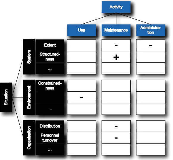
Figure 1: High-level view on an activity-based quality model as a matrix

Because facts are a composite of an entity and an attribute, the organisation in a hierarchy is straightforward. Hierarchical relationships between entities do usually already exist. The top-level in Figure 1 is the Situation of the software development project, which denotes the root for all entities of the system as well as entities from its environment. In the example, it contains the System, the system’s Environment and the development Organisation. Again, these entities need to be further refined. For example, the system could consist of the source code as well as the executable. All of these entities can be described with attributes, e.g., the STRUCTUREDNESS of the System. In principle, there could be more complex relationships instead of hierarchies, but modelling and finding information tends to be easier if such complex relationships are mapped to hierarchies.

The two hierarchies, the fact tree and the activity tree, together with the impacts of the facts on the activities can then be visualised using a matrix as in Figure 1. The fact tree is shown on the left, the activity tree on the top. The impacts are depicted by entries in the matrix where a “+” denotes a positive and a “–” a negative impact.

The associations between facts in the fact tree can have two different meanings. Either an entity is a part or a kind of its super-entity. Along the inheritance associations, parts and attributes are inherited. Hence, it allows a more compact description and prevents omissions in the model. For example, naming conventions are valid for all identifiers no matter whether they are class names, file names, or variable names.

Having defined all these entries in the ABQM, we can specify which activities we want to support and which influencing facts need to be analysed. In terms of the above example, if we want to support the activity Modification, we know that we need to inspect the identifiers for their consistency.

Another way of looking at ABQMs is as GQM patterns [9, 10]. The activity defines the goal and the facts are questions for that goal that are measured by certain metrics in a defined assessment. In the example, the goal is to evaluate the modification activity that is analysed by asking the question “How consistent are the identifiers?”, which is asked in an assessment.

There exists a prototype tool to define this kind of large and detailed quality models [4]. Besides the easier creation and modification of the model, this has also the advantage that we can automate certain quality assurance tasks. For example, by using the tool we can automatically generate customised review guidelines for specific views.

3 Assessment and Prediction Approach

Although activity-based quality models have proven to be useful in practice, there is no systematic measurement approach for them. Hence, there are no quantitative assessments and predictions possible so far. We propose an approach that can be used for systematically deriving assessment and prediction models from an activity-based quality model.

3.1 Aim and Basic Idea

The general aim of the approach is to provide quality managers with a systematic method to derive assessments and predictions from an activity-based quality model. In the ABQM, there are definitions of what quality means with respect to different situations, artefacts, and considered activities. At present, we give a textual description in the quality model that specifies how a fact could be assessed. For example, the fact described by [Method$\,|\,$REDUNDANCY] contains the following assessment description: “This fact can be assessed manually or semi-automatically. For the automatic assessments there are tools such as ConQAT or CCFinder to detect redundant parts of the source code.” This information is useful for quality assurance planning but cannot directly be used for an overall assessment, let alone prediction.

Moreover, as the basic principle of activity-based quality models is that the most important question in quality is how well activities can be performed on and with the system, not only facts but also activities should be assessed and predicted from the knowledge of facts and impacts. At present, activity-based quality models only make the qualitative statement whether an impact is positive or negative. This is suitable for rough assessments only. More comprehensive and precise assessments of the current state and prediction of future states need a more sophisticated approach. It has to systematically help using the given relationships and enriching them with quantitative information. In terms of measurement scales, we move from an ordinal scale to an interval scale or higher.

As most facts and especially the relationships between facts and activities have an associated uncertainty, statistical methods are necessary. The two major reasons are

1. that we cannot determine the exact relationship but can derive an uncertain range and

2. measured values can be uncertain, e.g., values from expert opinion.

Moreover, the statistical method needs to be able to directly model the dependencies of different factors from the quality model. We identified Bayesian networks as most suitable for that task.

3.2 Bayesian Networks

Bayesian networks, also known as Bayesian belief nets or belief networks, are a modelling technique for causal relationship based on Bayesian inference. They are represented as a directed acyclic graph with nodes for uncertain variables and edges for directed relationships between the variables. This graph models all the relationships abstractly. A hypothetical example with the 3 variables Code Complexity, Testing Effort, and Number of Field Failures is given in Figure 2. The code complexity influences the testing effort and the number of field failures of a software. The testing effort also impacts the number of failures.

Figure 2: A simple example Bayesian network

For each node or variable there is a corresponding node probability table (NPT). These tables define the relationships and the uncertainty of these variables. The variables are usually discrete with a fixed number of states. For each state, it gives the probability that the variable is in this state. If there are parent nodes, i.e., a node that influences the current node, it defines these probabilities in dependence on the states of the parents. An example for the variable Number of Field Failures is shown in Table 1. It specifies all combinations, e.g., that the Number of Field Failures is with a probability of 60% in the state “$>100$” if both parents are in the state low, and with 40% in “$>100$” if the testing effort is high and the code complexity is low.

Table 1: An example NPT for the variable Number of Field Failures with two states and two parents

Testing Effort		low			high
Code Complexity	low	med	high	low	med	high
$<100$	0.4	0.3	0.2	0.6	0.55	0.5
$>100$	0.6	0.7	0.8	0.4	0.45	0.5

The process of building a Bayesian network contains the identification of important variables that shall be modelled, representing them as nodes, constructing the topology and specifying the NPTs. Each of these steps is important and non-trivial. First, the identification of important variables includes the assumption that the model builder can decide on some basis what is important. In many cases, this is not clear beforehand. One possibility is to include many variables and use sensitivity analysis to remove insignificant ones. A model of the complete situation is usually not feasible, because the network becomes too complex, very elaborate to build, and most often there is no knowledge available about several variables.

Second, the creation of the topology utilises the assumption that the model builder can decide on the dependence and independence of the identified variables. In the process of building the Bayesian network, especially for independence assumptions (i.e., missing edges in the graph), detailed justifications should be given. Third, the problem of constructing NPTs is widely acknowledged in the literature [11]. A major part of this problem is that it involves defining quantitative relationships between variables. There are various possible methods for this quantification such as a probability wheel or regression from empirically collected data. All methods have their pros and cons.

It is important to note that each of these steps is important and errors in each of these steps can have a large effect on the outcome. Bayesian networks and the corresponding tool support make it easy to build models and get quantitative results. However, one needs to be aware that many assumptions are embedded in a Bayesian network that need to be validated before it can be trusted.

3.3 Four Steps for Network Building

We propose a four-step approach for building a Bayesian network as assessment and prediction model derived systematically from an activity-based quality model. The resulting Bayesian network contains three types of nodes:

• Activity nodes that represent activities from the quality model

• Fact nodes that represent facts from the quality model

• Indicator nodes that represent metrics for activities or facts

We need four steps to derive these nodes from the information of the ABQM. First, we identify the relevant activities with indicators based on the assessment or prediction goal. Second, influences by sub-activities and facts are identified. This step is repeated recursively for sub-activities. The resulting facts together with their impacts are modelled. Third, suitable indicators for the facts are added. Fourth, the node probability tables (NPT) are defined to reflect the quantitative relationships. Having that, the Bayesian network can be used for simulation by setting values for any of the nodes. However, we first describe the four steps in more detail.

Step 1

The first step is a goal-based derivation of relevant activities and their indicators. We use GQM [9] to structure that derivation. We first define the assessment or prediction goal, for example, optimal maintenance planning or optimisation of security assurance. The identification and resolution of conflicting goals is out of scope of this method. The goal leads to relevant activities, such as maintenance or attack. This is refined by stating questions that need to be answered to reach that goal. For example, how high will be the maintenance effort over the next year or how often will there be a successful attack in the next year? Finally, we derive metrics or indicators that allow a measurement to answer the question. In the examples, it can be the average change effort or the number of harmful attacks over the next year.

Step 2

In the second step, we use the quality model to identify the other factors that are related to the identified activities. There are two possibilities:

1. There are sub-activities of the identified activities.

2. There are impacts from facts to the identified activities.

We repeat this recursively for the sub-activities until all facts are collected that have an impact on the activities sub-tree below the identified activity. For each activity we immediately see the impacts and hence the corresponding facts. All activities and facts identified this way are modelled as nodes in the Bayesian network. We add edges from sub-activities to super-activities and from facts to activities on which they have an impact. Figure 3 gives an abstract overview of that mapping from the quality model to the Bayesian network.

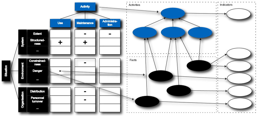
Figure 3: Mapping of quality model elements to Bayesian network elements. The dashed arrows indicate examples for mappings.

Step 3

In the third step, we add additional nodes as indicators for each fact and activity node that we want a measurement for. In the first step, we defined the indicator for our relevant activity. Hence, we can add additional indicators for sub-activities if needed. In any case, there need to be at least one indicator for each fact that is modelled. There might be a precise description in the quality model already. Otherwise, we need to derive our own metric or use an existing one from the literature. The indicator does not have to be measured automatically, but manual reviews can also be included in the assessment. The edges are directed from the activity and fact nodes to the indicators, i.e., the indicators are dependent on the facts and activities as an indicator is only an expression of the underlying factor it describes.

A main advantage of using an ABQM as a basis for the Bayesian network is that it prescribes its topology. One of the prime points of such quality models is to qualitatively describe the relationships between different factors that are relevant for software quality. We rely on that and assume that all dependencies have been modelled and that all other factors are independent. On the one hand, this constrains the validity of the results of the Bayesian network by the validity of the ABQM. On the other hand, it frees the network builder from reasoning about independence and dependence.

Step 4

Finally, the fourth step enriches the Bayesian network with quantitative information. This includes defining node states as well as filling the NPT for each node. The activity and fact nodes are usually modelled as ranked nodes, i.e., in an ordinal scale. The most common example is the scale containing low, medium, and high. This has advantages in evaluation and aggregation. The evaluation is easier as not precise numbers have to be determined but coarse-grained levels. These levels actually reflect much more the high uncertainty in the data. In aggregating over nodes (up the hierarchy in the activity tree) coarse-grained ranked data is also more simple to handle. It is easier to define an aggregation specification for only a few levels in an ordinal scale than for continuous data.

To define the NPT, we use an approach proposed by Fenton, Neil and Galan Caballero [12]. The basic idea is to formalise the behaviour observed with experts that have to estimate NPTs. They usually estimate the central tendency or some extreme values based on the influencing nodes. The remaining cells of the table are then filled accordingly. This is similar to linear regression where a Normal distribution is used to model the uncertainty. We use the doubly truncated Normal distribution (TNormal) that is only defined in the $[0,1]$ region. It allows to model a variety of shapes depending on the mean and variation. For example, it renders it possible to model the NPT of a node by a weighted mean over the influencing nodes.

The node states of indicator nodes depend on the scale of the indicator used. This often will be continuous or discrete interval states such as lines of codes in intervals of a hundred or a thousand. The NPTs of the indicator nodes are then defined using either common industry distributions or information from company-internal measurements. For example, typical LOC distributions can be accumulated over time. The influence of the activity or fact node it belongs to can be modelled in at least two ways:

• partitioned expressions

• arithmetic expressions

The latter describes a direct arithmetical relationship from the level in the activity or fact node to the indicator. Using a partitioned expression, the additional uncertainty can be expressed by defining probability distributions for each level of the node.

3.4 Usage of the Bayesian Network

A major feature of Bayesian networks is their capability to simulate different scenarios. Having built the Bayesian network based on the ABQM, we can ask “what if?” questions. These questions are formulated in scenarios that can be simulated and compared. A scenario involves adding additional information to the model, more specifically, adding an observation for a node. This way, the uncertainty is removed and the consequences for the other nodes can be calculated. In a Bayesian network it is possible to do forward as well as backward inference, i.e., information can be added to any node and the effect is calculated in any direction of the graph.

A first straightforward scenario is to add the currently measured values for the fact indicator nodes. This will drive the calculation up to the activities and the activity indicator node. The activity indicator node then shows the probability distribution for its value, i.e., the value of the activity. Afterwards changes can be made to the fact indicator nodes in other scenarios to reflect possible changes and their effect on the activity can be predicted. A further interesting scenario is to set a desired value for the activity indicator and let the network calculate the most probable explanation in the fact indicators. It provides the values that should be reached in order to fulfil the goal.

4 Initial Evaluation

The approach presented above can be used in various contexts to answer assessment and prediction questions. In this section, we provide an initial evaluation by applying the approach to several publicly available data sets as well as automatically collectable measures for an open source system.

4.1 Goal

We provide an exemplary application of the approach based on a small extract of our quality model for maintainability for which there is public data available, and on our model for security for which we collect measures from an open source system. The examples demonstrate the basic principles of the approach on real data sets. This way, we analyse whether the approach is feasible in an almost realistic setting. The predictive validity in the examples can give an indication of the usefulness of the approach, because we expect an improvement over industry average values at least.

At present, we cannot provide a complete validation of the assessment and prediction approach because this would involve measuring a large number of facts from the quality model in order to take full advantage from the knowledge contained in it. This data is not available in public data sets. Measuring this at a company will need time and effort. Only then a sensible analysis of the predictive validity and comparisons with other prediction models are possible.

4.2 Maintainability Cases

The first part of the examples deals with the analysis of maintainability. We follow the IEEE and define maintainability as follows: “The ease with which a software system or component can be modified to correct faults, improve performance or other attributes, or adapt to a changed environment.” [13]

4.2.1 Context

The 4 systems under analysis for maintainability were developed by NASA in the projects CM1, KC1, KC3, and KC4 for which the data has been publicised [14]. The characteristics of these projects are summarised in Table 2. Various metrics, including the McCabe and Halstead metrics, have been collected in these projects. The projects were selected for this analysis because their data is openly available and effort data per defect was collected. Hence, the selection criterion was opportunistic. Nevertheless, the diversity of sizes, functionality, and programming language in the set of analysed systems is sufficient to generalise the experiences to other systems.

Table 2: Characteristics of the projects used in the maintainability cases

Project	Size (LOC)	Lang.	Function
CM1	16,903	C	Space craft instrument
KC1	42,963	C++	Ground system
KC3	7,749	Java	Satellite data processing
KC4	25,436	Perl	Subscription server

As the quality model, we use the activity-based quality model for maintainability from [4]. It contains a complete activity tree for maintenance as well as about 200 facts with an impact on those activities. The NASA data sets do not contain data for all of these facts; hence, we select a small set of facts and corresponding activities to predict maintainability. The choice was therefore guided by the availability of the data. The actual maintainability can be judged for these projects, because the effort for several changes has been documented. We will use this as our surrogate measure.

For modelling the Bayesian network, we use the tool AgenaRisk. It provides a complete tool environment for Bayesian networks including the usage of expressions for describing the NPT and sensitivity analysis.

4.2.2 Procedure

The first step in our assessment and prediction approach is to identify the relevant activities and corresponding indicators (metrics) in a GQM-like procedure. We want to analyse maintainability and we assume that the quality manager is interested in the question of how high the maintenance efforts will be on average in the future. This information helps in planning the maintenance team. Hence, we formulate the goal as “Planning of future maintenance efforts”. We can directly identify the activity Maintenance in that goal. To further operationalise that, we define the corresponding question as “What will be the maintenance effort per change request?”. This information, together with a prediction of the yearly number of change requests, would give a good basis for maintenance planning. However, we concentrate only on the question about the effort per change request. This leads us straightforwardly to the metric “average effort per change request”.

In the second step, we start building the Bayesian network. We look at the maintainability model and find no direct impacts on Maintenance that should be considered here. However, we find 10 sub-activities including the following 3 that we analyse further: Quality Assurance, Implementation and Analysis. All three have impacts from facts but having in mind the available data, we ignore these and use the further sub-activities Testing, Modification and Comprehension with its child Code Reading. We create nodes for these activities and connect them with edges corresponding to their hierarchy. They can be seen in Figure 4 in the box “Activities”.

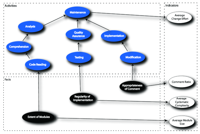
Figure 4: The topology of the Bayesian network for the maintainability cases

We only include 3 impacts on each of the lowest level activities chosen so far because we can find corresponding data in the NASA data sets. These facts together with their impacts are:

• [Module$\,|\,$EXTENT] $\stackrel{{\scriptstyle-}}{{\longrightarrow}}$ [Code Reading]
  The size of a module has an impact on reading the code of the module. In essence, the larger the module, the longer it takes to read it.

• [Implementation$\,|\,$REGULARITY] $\stackrel{{\scriptstyle+}}{{\longrightarrow}}$ [Testing]
  An implementation is regular if it does not use unnecessarily nested branches. This complex structure would render coverage by tests more difficult.

• [Comment$\,|\,$APPROPRIATENESS] $\stackrel{{\scriptstyle+}}{{\longrightarrow}}$ [Modification]
  Comments need to appropriately describe the code it is associated with.

We add these facts as nodes in the Bayesian network into the box “Facts” in Figure 4. The impacts are included as the arrows from the facts to the activities. There are further impacts conceivable, but we restrain them to the impacts available in the used maintainability model [4].

The indicators that are identified in the fourth step of the approach are taken from the available data of the data set. We only use one indicator per fact although we are aware that each fact has more aspects that should be covered. For the Extent of Modules, we use the indicator Average module size given in LOC. The Regularity of the Implementation is indicated by the Average Cyclomatic Complexity. This is not a particularly good indicator as it only gives a number for the decision points in the implementation. In contrast, a manual review could far better decide whether the implementation is regular. However, we have no access to review results. A similar reasoning holds for the indicator Comment Ratio for the fact Appropriateness of Comments. The proportion of the comments in relation to the other code is only of minor importance in comparison with the semantic appropriateness. However, we do not have access to such a semantic judgement. The indicators can be found in Figure 4 on the right-hand side in the box “Indicators”.

A difficult problem in general with Bayesian networks is the definition of the node probability tables (NPT) [11]. Network builders can use various methods to define these NPTs, which we do not describe here in detail. For the approach, we can simplify the problem to 2 cases:

• Activity and fact NPTs

• Indicator NPTs

The NPTs for the activities and facts can be assumed as uniformly distributed unless there is additional knowledge. The impacts are only modelled as direct influence. Here, a special method for ranked nodes [12] can be applied that simplifies the task. For example, the node Maintenance is modelled by the following distribution as its NPT:

$$\mbox{TNormal}\left[\frac{\mbox{Analysis}+\mbox{Quality\ Assurance}+\mbox{Implementation}}{3},\frac{1}{3},0.001\right]$$ (1)

The values of the three nodes Analysis, Quality Assurance, and Implementation are averaged with the implicit weight 1 each. The 1/3 gives the normalisation and 0.001 is the variance.

For the indicator NPTs either empirically investigated distributions of the company or industry average distribution should be used. This forms the distribution of the indicator values under uncertainty without any observations. The indicator node Comment Ratio is shown as an example in Table 3. It gives the NPT as an partitioned expression depending on the state of the parent node Appropriateness of Comments.

Table 3: NPT of the indicator node Comment Ratio

Appropriateness of Comments	Expressions
Low	TNormal[0.01,1,0.03]
Medium	TNormal[0.1,1,0.05]
High	TNormal[0.25,1,0.1]

For the average effort of a change, we refer to [15] that gave a mean defect removal cost of 27.4 person-hours with minimum 3.9 and maximum 66.6. Although a change does not always have to be a defect removal, it is precise enough for the initial evaluation. For the distributions of the other indicators, no published distributions were available. Hence, our own expert opinion was used as a basis.

4.2.3 Results and Discussion

Figure 5: The Bayesian network for KC1 in AgenaRisk. The standard scenario is shown in light grey, the KC1 scenario in dark grey.

Figure 5 shows a screenshot from AgenaRisk as an example. The light-grey values describe the general scenario in which no observations have been made. The dark-grey values are for the KC1 scenario in which for the three fact indicators the real measured values are set as observations. Table 4 summarises the used observation data and the results from the Bayesian network for all 4 maintainability cases. It shows the observed values for the comment ratio, the average cyclomatic complexity, and the average module size in LOC. These were fixed in their corresponding scenarios. This has effects on the rating of the facts and in turn on the activities. The most interesting value, however, is the average change effort. In the general scenario, this variable has a mean value of 27 with a standard deviation of 12.1. The table gives the predicted average change effort in person hours together with the standard deviation as well as the actually observed average change effort.

Table 4: Observations and results for the maintainability cases

	CM1	KC1	KC3	KC4
Comment ratio	0.25	0.02	0.08	0.00
Avg. cyclomatic complexity	5.18	2.84	3.45	10.05
Avg. module size	33.47	20.39	16.92	203.49
Predicted avg. change effort	15.9	19.4	19.2	36.1
Standard deviation	8.5	9.8	9.8	12.1
Observed avg. change effort	6.0	21.7	24.8	12.1

The 4 cases show 3 different types of results. For KC1 and KC3, the predictions are very close to the observed values with a difference of 2.3 and 5.6 person-hours per change, respectively. For both predictions, the observed values are well inside the standard deviation. Hence, in these cases, the predictions are reasonably accurate.

For CM1, the additional information about the measured values shifts the distribution to the left. The mean decreases to 15.9 with a standard deviation of 8.5. This is a deviation of 9.9 from the observed value. However, it is much closer than the industry standard of 27. Hence, it is an improvement in comparison to just using standard numbers.

In the case of KC4, the industry standard 27 [15] would have been closer than the prediction of 36.1 which constitutes a difference of 24 from the actual value. This is not even inside the standard deviation. The prediction is far too pessimistic. The reason for the large difference between the prediction and the real value can be three-fold. First, the effort distribution from [15] might not be appropriate for the NASA environment. Second, it might also be the case that the data in the NASA data sets do not use exactly the same measures as in [15]. The degree to which additional efforts for re-inspection and re-testing are included could vary. Third, several more factors than the 3 considered might have an influence on the maintenance effort. The quality model contains many explanations in terms of facts that should be investigated. Especially for KC4, there are probably other factors that decrease the change effort in such a way. For example, the capabilities of the developers are known to have a large effect on development productivity [16]. However, we cannot include this as a fact in this case, because we have no data available.

4.3 Security Case

The second part of the examples looks at security. We use the following definition of Avizienis et al.: “Security is a composite of the attributes of confidentiality, integrity, and availability, requiring the concurrent existence of 1) availability for authorized actions only, 2) confidentiality, and 3) integrity with ‘improper’ meaning ‘unauthorized.”’ [17]

4.3.1 Context

The servlet container Tomcat is the reference implementation of the Java servlet and JSP specification by the Apache Software Foundation. Its main goal is to deliver HTTP responses dynamically assembled based on an HTTP request. For this, Tomcat is one of the most used systems in the world. We employ version 6.0 of Tomcat, which implements the Java servlet specification 2.5 and the JSP specification 2.1. The initial version 6.0.0 was released in December 2006. The current version 6.0.20 dates from May 2009. It consists of over 300 KLOC of Java code and it is in real production on many sites.

A software application with such a fundamental role in Java web applications has special responsibilities in the management of vulnerabilities. Therefore, the Apache foundation openly publishes the identified vulnerabilities. They can be found on the Tomcat website. This published list of vulnerabilities together with the availability of the source code for further analyses is the reason for selecting Tomcat for this example. Hence, the selection criterion was again opportunistic.

The ABQM used for the security case is the security model as described in [7]. This model uses a well-known hierarchy of attacks as activities and a collection of open security guidelines as facts. As modelling tool for the Bayesian network, we employ again AgenaRisk.

4.3.2 Procedure

We start with the first step of our assessment and prediction approach and identify the relevant activities and corresponding indicators. We analyse security, in particular the risk of vulnerabilities in the system. The risk can be the basis for deciding whether further security improvements need to be employed. Therefore, the goal is “Planning of further security improvements”. For security improvements, attacks on the system need to be confounded. Hence, the activity Attack need to be analysed. For the operationalisation, we define the question “How many vulnerabilities are there in relation to the software size?”. For the security improvement planning, it is not only important how many vulnerabilities there are but also whether this number is in a reasonable relation to the system size. It might be economically inadvisable to invest in removing all vulnerabilities. The corresponding metric vulnerability density that measures the number of vulnerabilities by source code size in KSLOC can be directly derived from the question.

In the second step of the prediction and assessment approach, we build the Bayesian network (see Figure 6). In the ABQM for security, there is the top-level activity Attack that we measure by the above derived vulnerability density. There are no direct impacts on this activity. Therefore, we break it down to Abuse of Functionality, Injection, and Resource Manipulation. The former is further refined into Functionality Misuse, the second into Format String Injection and Embedding Scripts in Non-Script Elements, the latter into Variable Manipulation. In the Bayesian network, nodes are created for these activities w.r.t. the given hierarchy.

We can include 8 impacts on these activities. The impacts are chosen so that their corresponding facts can be automatically measured by a bug pattern tool. We chose the open source tool FindBugs, because it is widely used and well evaluated. The facts used together with their impacts are:

• [Object$\,|\,$IMMUTABILITY] $\stackrel{{\scriptstyle-}}{{\longrightarrow}}$ [Variable Manipulation]
  When objects are not immutable the caller can change the contents of these objects which may have security implications. Hence, objects should be immutable if possible.

• [Field$\,|\,$LOCALITY] $\stackrel{{\scriptstyle-}}{{\longrightarrow}}$ [Variable Manipulation]
  A mutable static field could be changed by malicious code or by accident from another package. The field could be made package protected and/or made final to avoid this vulnerability.

• [Field$\,|\,$IMMUTABILITY] $\stackrel{{\scriptstyle-}}{{\longrightarrow}}$ [Variable Manipulation]
  When a static field is mutable or references mutable objects, these could be changed by malicious code.

• [Finalizer$\,|\,$LOCALITY] $\stackrel{{\scriptstyle-}}{{\longrightarrow}}$ [Functionality Misuse]
  Malicious code could call the method finalize if it is not declared protected while the object is still used and external resources could be closed too early.

• [Cookie$\,|\,$SANITATION] $\stackrel{{\scriptstyle-}}{{\longrightarrow}}$ [Format String Injection]
  If a web product does not properly protect assumed-immutable values from cookies, this can lead to modification of critical data.

• [Dynamic Web Page$\,|\,$SANITATION] $\stackrel{{\scriptstyle-}}{{\longrightarrow}}$ [Embedding Script in HTTP Headers]
  [Dynamic Web Page$\,|\,$SANITATION] $\stackrel{{\scriptstyle-}}{{\longrightarrow}}$ [Embedding Scripts in HTTP Query Strings]
  [Dynamic Web Page$\,|\,$SANITATION] $\stackrel{{\scriptstyle-}}{{\longrightarrow}}$ [XSS in Error Pages]
  If a web application does not sufficiently sanitise the data it is using in output, arbitrary content, including scripts, can be included by attackers.

In the fourth step of the approach, indicators are defined for all 8 impacts. The indicators in this case are all derived from FindBugs bug patterns that are summed if they only measure different aspects of the same fact and set into relation to the size of the system. Hence, we end up with a set of densities of detected bug pattern. Table 5 gives the used facts together with their associated bug patterns and the corresponding name of the density of the sum of the findings for these patterns. The final topology of the Bayesian net is shown in Figure 6.

Table 5: The mapping of facts to FindBugs patterns and metrics

Fact	FindBugs Pattern	Metric
[Object$\,|\,$IMMUTABILITY]	• May expose internal representation by returning reference to mutable object • May expose internal representation by incorporating reference to mutable object	OJI
[Field$\,|\,$LOCALITY]	• Field isn’t final and can’t be protected from malicious code • Field should be moved out of an interface and made package protected • Field should be package protected • Field isn’t final but should be	FDL
[Field$\,|\,$IMMUTABILITY]	• May expose internal static state by storing a mutable object into a static field • Field is a mutable array • Field is a mutable Hashtable	FDI
[Finalizer$\,|\,$LOCALITY]	Finalizer should be protected, not public	FZL
[Cookie$\,|\,$SANITATION]	HTTP cookie formed from untrusted input	COS
[Dyn. Web Page$\,|\,$SANITATION]	Servlet reflected cross site scripting vulnerability	DWS

Figure 6: The topology of the Bayesian network for the security case

There is little quantitative data published on vulnerabilities. Therefore, we use the data on vulnerability densities from Alhazmi, Malaiya, and Ray [18] who analysed several releases of Microsoft Windows and Red Hat Linux. On average, these systems had a known vulnerability density of 0.0054 with a minimum of 0.0022 and a maximum of 0.0112 vulnerabilities per KSLOC. There is no data available about what are average densities or even occurrences of specific bug patterns in software systems. Hence, we make the coarse assumption that we consider a density of 0.4 as normal for all defined indicators for the facts. That means that 4 occurrences of each of these bug patterns in 10 KSLOC is normal. We employed an exponential distribution as we assume that there is a high concentration in the lower areas of the distribution that decreases quickly in the higher areas.

4.3.3 Results and Discussion

Using the analysis tool ConQAT [19], we found that the whole Tomcat 6.0.0 source distribution contains 306,675 LOC of Java code, which correspond to 151,509 SLOC in 1030 files. This is the size baseline for all the following densities. The total number of published vulnerabilities of Tomcat is 24. However, we only consider the vulnerabilities rated as important and moderate because we assume that in other systems other vulnerabilities would not be counted as such. With this assumption the number is reduced to 11.

Table 6 contains the summarised results. First, the 6 indicators are given. These densities range from 0 to 1.14 occurrences per KSLOC. In the Bayesian network, this led to the prediction of 0.006 vulnerabilities per KSLOC with a standard deviation of 0.003. Actually observed in Tomcat over all 6.0 versions, we found a vulnerability density of 0.07 vulnerabilities per KSLOC.

Table 6: Observations and results for the security case. All densities are given in occurrences per KSLOC.

OJI density	1.14
FDL density	1.63
FDI density	0.06
FZL density	0.03
COS density	0.00
DWS density	0.00
Predicted vulnerability density	0.006
Standard deviation	0.003
Observed vulnerability density	0.070

Obviously, the prediction is not very accurate, but the distribution shifts in the correct direction as the mean of the distribution used for the vulnerability density is 0.0054. This effect is similar as in the CM1 case in section 4.2. The model cannot completely overcome deficiencies in the underlying distributions for the indicators.

Windows and Linux have 15–40 MSLOC, i.e., the are an order of magnitude larger than Tomcat. Hence, one explanation of the large difference could be that the used underlying distribution for the vulnerability is wrong and need to be improved with data from systems with other sizes. Another possibility is that the system size is a fact that needs to be considered. In this case, it seems that smaller systems have a higher vulnerability density. This could be explained by the fact that in Tomcat almost all parts of the system are exposed to external access. Therefore, the fact Size of Software might be introduced as an additional factor. However, experimenting with this additional fact showed that it cannot reach accurate prediction as it is still constrained by the vulnerability density distribution.

The large difference can also mean that our chosen metric vulnerability density is not suitable as it seems to be strongly dependent on the system size, type, or both. Hence, more advanced metrics such as breach rates or cost to breach [20] should be used. These measures are, however, significantly harder to measure.

4.4 Discussion

The foremost goal of these examples was not to show predictive validity but to investigate the general feasibility of the assessment and prediction approach. Nevertheless, in two of the maintainability cases, we were able to come to accurate predictions although we had little knowledge about the actual system. Furthermore, we saw that it is possible to build a Bayesian model with reasonable effort. The four-step approach gives direct guidance for most of the network building. However, setting up the NPTs is still a challenge. There are usually several possibilities how a relationship can be expressed and with how much uncertainty it should be afflicted. This needs expert opinion and experimentation. Nevertheless, AgenaRisk provides sophisticated tool support to find easier ways to define an NPT.

Another problem encountered in the analysed cases was to find a reasonable empirical data basis for the distribution of the indicators. For the facts and activities, it is sufficient to employ rather coarse-grained ranked states and the good tool support helps in defining corresponding distributions. For the indicators, a good data basis or distributions from the literature are crucial.

As our ABQMs can get very large with a few hundreds of model elements, it remains to be evaluated whether the approach scales when the quality model is fully mapped to a Bayesian network. Probably a selection of a subset of the quality model is necessary first.

Furthermore, it is important to note that a more in-depth validation of a resulting Bayesian network is necessary in order to ensure that all parts – topology, node states, and NPTs – represent the interdependencies of the quality factors good enough so that a valid statement about the quality of the software system can be made. This is not covered by these examples but has to be the next step.

The usage of the proposed approach, however, has benefits beyond assessing a quality goal. If we are able to calibrate the model and establish sufficient accuracy in the Bayesian network, we will be able to calculate low level goals for quality goals. For example, we can infer requirements for the indicators of the maintainability cases for a given goal for the average change effort. A required average change effort of only 10 person-hours has the most likely explanation in a comment ratio of 0.3, an average cyclomatic complexity of 6.4, and an average module size of 64 LOC. This can be used to guide development. Finally, also requirements specification is supported by this approach as quality requirements now can use the given indicators to specify assessable requirements.

5 Related Work

The basic idea to use Bayesian networks for assessing and predicting software quality has been developed foremost by Fenton, Neil, and Littlewood. They introduced Bayesian networks as a tool in this area and applied it in various contexts related to software quality. In [21] they formulate a critique on current defect prediction models and suggest to use Bayesian networks. Other researchers also used Bayesian networks for software quality prediction similarly [22, 23]

The work closest to the approach proposed in this paper is [24]. The authors discuss quality models such as the ISO 9126 [2] and their problems such as the undefinedness of the relationships in such a model. They aim at solving these problems by defining Bayesian networks for quality attributes directly. Our work differentiates in using a defined structure for quality models that contain far more details as common quality models. This structure and detail allows a straightforward derivation of a Bayesian network from the quality model. This has the advantage that the basic quality model can also be used for other purposes then prediction such as the specification of quality requirements.

Beaver, Schiavone, and Berrios [25] also used a Bayesian network to predict software quality including diverse factors such as team skill and process maturity. In his thesis [26], Beaver even compared the approach to neural networks and Least Squares regressions that both were outperformed by the Bayesian network. However, they did not rely on a structured quality model as in our approach.

An earlier version of this paper was published in [27]. It already contained the 4-step approach as described in this paper. However, we added 3 additional projects to the maintainability case and a completely new security case in order to validate the applicability of the approach more broadly.

6 Conclusions

A high goal in software quality management is the reliable quantitative assessment and prediction of software quality. Many efforts in building assessment and prediction models have given insights in the usefulness but also the constraints of such models. However, these models have not been tightly integrated into other quality management activities. Activity-based quality models have proven in practice to be a solid foundation for defining quality on a detailed level. However, quantitative analyses have not been directly possible so far.

Bayesian networks have been shown to provide promising results in quality predictions. Because of that and their clear structuring that can straightforwardly reflect the structure of activity-based quality models, a four-step approach for transferring activity-based quality models to Bayesian networks was proposed. It allows to systematically construct a Bayesian network that uses the knowledge encoded in the quality model to provide information about a given assessment or prediction goal. In the terminology of [28], we use a quality definition model (the ABQM) and enrich it with a quality assessment and quality prediction model (the Bayesian Network).

Although not fully validated, we demonstrated the approach in a study using real NASA project data and automatically measured bug patterns of the Tomcat servlet container. The examples showed the applicability of the approach to such projects and could improve the prediction in comparison to industry standard values. For 2 of the 5 cases, the predictions were accurate despite the usage of literature values as basis for the distributions only.

The use of Bayesian networks opens many possibilities. Most interestingly, after building a large Bayesian network, a sensitivity analysis of that network can be performed. This can answer the practically very relevant question which of the factors are the most important ones. It would allow to reduce the measurement efforts significantly by concentrating on these most influential facts.

We plan to apply this approach in future case studies at our industrial partners in order to further validate the approach. A comprehensive analysis of the predictive validity is necessary to judge the usefulness of the approach and to compare it with other means for assessment and prediction.

7 Acknowledgments

This work has partially been supported by the German Federal Ministry of Education and Research (BMBF) in the project QuaMoCo (01 IS 08023B). I would like to thank the anonymous reviewers at PROMISE for feedback on an earlier version and Vic Basili, Sebastian Winter, and the anonymous IST reviewers for helpful suggestions for this version.

References

- [1] S. Wagner, F. Deissenboeck, An integrated approach to quality modelling, in: Proc. 5th International Workshop on Software Quality (5-WoSQ), IEEE Computer Society Press, 2007.
- [2] ISO 9126-1, Software engineering – Product quality – Part 1: Quality model, 2001.
- [3] B. Kitchenham, S. L. Pfleeger, Software quality: The elusive target, IEEE Software 13 (1) (1996) 12–21. doi:http://dx.doi.org/10.1109/52.476281.
- [4] F. Deissenboeck, S. Wagner, M. Pizka, S. Teuchert, J.-F. Girard, An activity-based quality model for maintainability, in: Proc. 23rd International Conference on Software Maintenance (ICSM ’07), IEEE Computer Society Press, 2007.
- [5] S. Wagner, K. Lochmann, S. Winter, A. Goeb, M. Klaes, Quality models in practice: a preliminary analysis, in: Proc. 3rd International Symposium on Empirical Software Engineering and Measurement (ESEM ’09), IEEE Computer Society, 2009.
- [6] S. Winter, S. Wagner, F. Deissenboeck, A comprehensive model of usability, in: Proc. Engineering Interactive Systems 2007, Vol. 4940 of LNCS, Springer-Verlag, 2008, pp. 106–122.
- [7] S. Wagner, D. Méndez Fernández, S. Islam, K. Lochmann, A security requirements approach for web systems, in: Proc. Quality Assessment in Web (QAW 2009), CEUR, 2009.
- [8] ISO/IEC 14764, IEEE Std. 14764-2006, Software Engineering – Software Life Cycle Processes - Maintenance, 2006.
- [9] V. R. Basili, G. Caldiera, H. D. Rombach, Goal question metric paradigm, in: J. C. Marciniak (Ed.), Encyclopedia of Software Engineering, Vol. 1, John Wiley & Sons, 1994.
- [10] M. Lindvall, P. Donzelli, S. Asgari, and V. Basili. Towards reusable measurement patterns, in: Proc. 11th IEEE International Software Metrics Symposium, IEEE Computer Society, 2005.
- [11] N. Fenton, M. Neil, Managing risk in the modern world. Applications of Bayesian networks, Knowledge transfer report, London Mathematical Society (2007).
- [12] N. E. Fenton, M. Neil, J. G. Caballero, Using ranked nodes to model qualitative judgments in Bayesian networks, IEEE Transactions on Knowledge and Data Engineering 19 (10) (2007) 1420–1432.
- [13] IEEE standard glossary of software engineering terminology, IEEE Std 610.12-1990 (1990).
-
[14]
NASA IV&V Facility, Metrics data program.
URL http://mdp.ivv.nasa.gov/ - [15] S. Wagner, A literature survey of the quality economics of defect-detection techniques, in: Proc. 5th ACM-IEEE International Symposium on Empirical Software Engineering (ISESE ’06), ACM Press, 2006.
- [16] B. W. Boehm, C. Abts, A. W. Brown, S. Chulani, B. K. Clark, E. Horowith, R. Madachy, D. Reifer, B. Steece, Software Cost Estimation with COCOMO II, Prentice Hall, 2000.
- [17] A. Avizienis, J.-C. Laprie, B. Randell, C. Landwehr, Basic concepts and taxonomy of dependable and secure computing, IEEE Transactions on Dependable and Secure Computing 1 (1) (2004) 11–33. doi:10.1109/TDSC.2004.2.
- [18] O. Alhazmi, Y. Malaiya, I. Ray, Security vulnerabilities in software systems: Security vulnerabilities in software systems: A quantitative perspective, in: Data and Applications Security 2005, Vol. 3654 of LNCS, Springer-Verlag, 2005, pp. 281–294.
- [19] F. Deissenboeck, E. Juergens, B. Hummel, S. Wagner, B. Mas y Parareda, M. Pizka, Tool support for continuous quality control, IEEE Software 25 (5) (2008) 60–67. doi:http://dx.doi.org/10.1109/MS.2008.30.
- [20] S. E. Schechter, Toward econometric models of the security risk from remote attack, IEEE Security and Privacy 3 (1) (2005) 40–44. doi:http://doi.ieeecomputersociety.org/10.1109/MSP.2005.30.
- [21] N. E. Fenton, M. Neil, A critique of software defect prediction models, IEEE Transactions on Software Engineering 25 (5) (1999) 675–689. doi:http://dx.doi.org/10.1109/32.815326.
- [22] S. Amasaki, Y. Takagi, O. Mizuno, T. Kikuno, Constructing a Bayesian belief network to predict final quality in embedded system development, IEICE Transactions on Information and Systems E88-D (6) (2005) 1134–1141.
- [23] E. Perez-Minana, J. Gras, Improving fault prediction using Bayesian networks for the development of embedded software applications, Software Testing Verification and Reliability 16 (3) (2006) 157.
- [24] M. Neil, B. Littlewood, N. Fenton, Applying Bayesian belief networks to systems dependability assessment, Safety Critical Systems Club Newsletter 8 (3).
- [25] J. M. Beaver, G. A. Schiavone, J. S. Berrios, Predicting software suitability using a bayesian belief network, in: Proc. Fourth International Conference on Machine Learning and Applications, IEEE Computer Society, 2005, pp. 82–88. doi:http://doi.ieeecomputersociety.org/10.1109/ICMLA.2005.52.
- [26] J. M. Beaver, A life cycle software quality model using bayesian belief networks, Ph.D. thesis, University of Central Florida (2006).
- [27] S. Wagner, A Bayesian network approach to assess and predict software quality using activity-based quality models, in: Proc. 1st International Conference on Predictor Models in Software Engineering (PROMISE ’09), ACM Press, 2009.
- [28] F. Deissenboeck, E. Juergens, K. Lochmann, S. Wagner, Software quality models: Purposes, usage scenarios and requirements, in: Proc. 7th International Workshop on Software Quality (WoSQ ’09), IEEE Computer Society, 2009.