Bridges in Complex Networks

Abstract

A bridge in a graph is an edge whose removal disconnects the graph and increases the number of connected components. We calculate the fraction of bridges in a wide range of real-world networks and their randomized counterparts. We find that real networks typically have more bridges than their completely randomized counterparts, but very similar fraction of bridges as their degree-preserving randomizations. We define a new edge centrality measure, called bridgeness, to quantify the importance of a bridge in damaging a network. We find that certain real networks have very large average and variance of bridgeness compared to their degree-preserving randomizations and other real networks. Finally, we offer an analytical framework to calculate the bridge fraction , the average and variance of bridgeness for uncorrelated random networks with arbitrary degree distributions.

A bridge, also known as cut-edge, is an edge of a graph whose removal disconnects the graph, i.e., increases the number of connected components (see Fig. 1, red edges) bollobas1998modern. A dual concept is articulation point (AP) or cut-vertex, defined as a node in a graph whose removal disconnects the graph behzad1972introduction; harary1969graph. Both bridges and APs in a graph can be identified via a linear-time algorithm based on depth-first search tarjan1972depth (see Supplemental Material Sec.I for details) and represent natural vulnerabilities of real-world networks. Analysis of APs has recently provided us a new angle to systematically investigate the structure and function of many real-world networks tian2016articulation. This prompts us to ask if similar analysis can be applied to bridges.

Note that bridge is similar but different from the notion of red bond introduced in percolation theory to characterize substructures of percolation clusters on lattices pike1981order. To define a red bond, we consider the percolation cluster as a network of wires carrying electrical current and we impose a voltage drop between two nodes in the network. Then red bonds are those links that carry all current, whose removal stops the current. The definition of bridges does not require us to impose a voltage drop on the network. Instead, it just concerns the connectivity of the whole network.

Despite that bridges play important roles in ensuring the network connectivity, the notion of bridge has never been systematically studied in complex networks. What is the typical number of bridges in a random graph with prescribed degree distribution? Are the bridges in a real network overpresented or underpresented? How to quantify the network vulnerability in terms of bridge attack? In this Letter, we systematically address those questions in both real networks and random graphs.

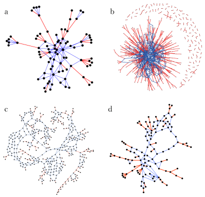
Figure 1: Bridges in real-world networks. Bridges (in red) are edges whose removal will increase the number of connected components in a graph. (a) Food web of Grassland dunne2002food; (b) The protein-protein interaction network of C. elegans simonis2009empirically; (c) A subgraph of the road network of California leskovec2015snap; (d) A subgraph of the power grid in three western states of US watts1998collective.

We first calculate the fraction of bridges ($f_{\mathrm{b}}:=L_{\mathrm{b}}/L$) in a wide range of real-world networks, from infrastructure networks to food webs, neuronal networks, protein-protein interaction (PPI) networks, gene regulatory networks, and social graphs. Detailed information of those networks can be found in Supplemental Material Sec. IV. Here $L_{\mathrm{b}}$ and $L$ denote the number of bridges and total links in a network, respectively. We find that many real networks have very small fraction of bridges, while a few of them (e.g., PPI networks) have very large fraction of bridges (Fig. 2a). To identify the topological characteristics that determine $f_{\mathrm{b}}$ in real networks, we compare $f_{\mathrm{b}}$ of a given network with that of its randomized counterpart. We first randomize each real network using a complete randomization procedure that turns the network into an Erdős-Rényi (ER) type of random graph with the number of nodes $N$ and links $L$ unchanged erdos1960evolution. We find that most of the completely randomized networks possess very different $f_{\mathrm{b}}$, compared to their corresponding real networks (Fig. 2a). This indicates that complete randomization eliminates the topological characteristics that determine $f_{\mathrm{b}}$. Moreover, we find that real networks typically display much higher $f_{\mathrm{b}}$ than their completely randomized counterparts (Fig. 2a). By contrast, when we apply a degree-preserving randomization, which rewires the edges among nodes while keeping the degree $k$ of each node unchanged, this procedure does not alter $f_{\mathrm{b}}$ significantly (Fig. 2b). In other words, the characteristics of a real network in terms of $f_{\mathrm{b}}$ is largely encoded in its degree distribution $P(k)$.

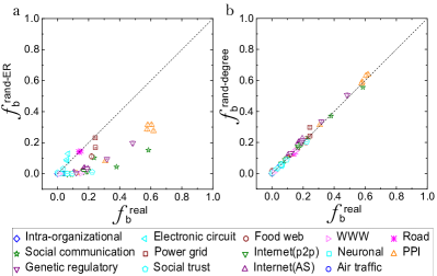
Figure 2: Fraction of bridges in real-world networks. The dashed lines are $y=x$. The error bars represent the standard deviation, calculated from 100 randomizations. (a) Complete randomization of real networks. (b) Degree-preserving randomization.

In order to quantify the importance of an edge in damaging a network, we define an edge centrality measure $B$, called bridgeness, for each edge in a graph as the number of nodes disconnected from the giant connected component (GCC) bollobas2001cambridge after the edge removal. By definition, if an edge is not a bridge or outside the GCC, it has zero bridgeness. Also, in the absence of GCC, all edges have zero bridgeness. We notice that bridgeness has been defined differently in the literature  nepusz2008fuzzy; gong2011variability; jensen2015detecting; cheng2010bridgeness (see Supplemental Material Sec.II). Here we define bridgeness based on the notion of bridge and we focus on the damage to the GCC, which is typically the main functional part of a network.

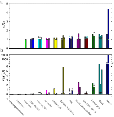
Figure 3: Average and variance of bridgeness in real-world networks. The bars represent the values of real networks and empty symbols represent the values of their degree-preserving randomizations. The error bars represent the standard deviation, calculated from 10 randomizations. (a) Average bridgeness. (b) Variance of bridgeness.

Bridgeness differentiates edges based on their structural importance. Consider all bridges that have non-trivial bridgeness, i.e., $B>0$. Denote their average and variance as $\langle B\rangle$ and $\mathrm{var}(B)$, respectively. We find that Word Wide Web (WWW) and road networks have much larger $\langle B\rangle$ than their randomized counterparts and other real networks (Fig. 3a). Moreover, those networks also have very large $\mathrm{var}(B)$ (Fig. 3b). The reason why road networks have very large $\langle B\rangle$ and $\mathrm{var}(B)$ is the presence of very long paths and the expense of constructing alternative paths. While for WWW, the reason is the presence of certain bridges that connect different large biconnected components in the GCC (see Supplemental Material Sec.IV). Here a biconnected component (BCC) is a connected subgraph where for any two nodes there are at least two paths connecting them that have no nodes in common other than these two nodes RN8034. (Note that by definition no bridges exist in a BCC.)

Since the bridge fractions in real networks are almost the same as their degree-preserving randomized counterparts, the difference of average bridgeness between real networks and their degree-preserving randomizations indicates variations of vulnerability of those networks in terms of bridge attack. Fig. 3a shows that certain types of networks, such as air traffic, road networks, social graphs and WWW, are more vulnerable, displaying much larger $\langle B\rangle$ than their randomizations. By contrast, the Internet at the autonomous system (AS) level and the Internet peer-to-peer (p2p) file sharing networks have smaller $\langle B\rangle$ than their randomized counterparts, indicating that those networks are robust from the bridge attack perspective.

The results of real-world networks prompt us to analytically decipher bridge structure for large uncorrelated random networks with prescribed degree distributions. To begin with, we adopt the local tree approximation, which assumes the absence of finite loops in the thermodynamic limit (i.e., as the network size $N\to\infty$) and allows only infinite loops tian2016articulation. This approximation leads to three important properties: (1) all finite connected components (FCCs) are trees, and hence all edges inside them are bridges; (2) there exists only one giant connected component (GCC) newman2001random, only one BCC (which has no bridges), and the BCC is a subgraph of the GCC; (3) subgraphs inside the GCC but outside the BCC are trees and all edges in those subgraphs are bridges cohen2000resilience; callaway2000network; newman2001random; dorogovtsev2008critical; mezard2009information; tian2016articulation.

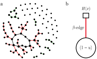
Figure 4: Demonstration of different types of edges. (a) The green lines, red lines and black lines represent $\alpha$-edges, $\beta$-edges and $\gamma$-edges, respectively. (b) Neighborhood of a $\beta$-edge. The red line is a $\beta$-edge and the black square and ellipse represent an FCC and the GCC, respectively, after the removal of the $\beta$-edge.

Based on the above considerations, we categorize all the edges in a graph into three types (Fig. 4a): (i) $\alpha$-edge: edges in FCCs, which are bridges; (ii) $\beta$-edge: edges inside the GCC but outside the BCC, which are also bridges; (iii) $\gamma$-edge: edges inside the BCC, which are not bridges. Hereafter we also use $\alpha$, $\beta$ or $\gamma$ to denote the probability that a randomly chosen edge is a $\alpha$-edge, $\beta$-edge, or $\gamma$-edge, respectively. By definitions, we have $\alpha+\beta+\gamma=1$, and $f_{\mathrm{b}}=\alpha+\beta$. Note that according to our definition of bridgeness, only $\beta$-edges have nontrivial bridgenesses, i.e., $B>0$.

The generating functions $G_{0}(x)=\sum_{k=0}^{\infty}P(k)x^{k}$ and $G_{1}(x)=\sum_{k=1}^{\infty}Q(k)x^{k-1}$ are very useful in calculating key quantities of random graphs, such as the mean component size and the size of GCC newman2001random. Here $Q(k)=kP(k)/c$, and $c=\sum_{k=0}\infty kP(k)$ is the mean degree. To calculate $\alpha$, $\beta$ and $\gamma$, we introduce the generating function $H_{1}(x)$ for the size distribution of the components that are reached by choosing a random edge and following it to one of its ends. (Note that the notation $H_{0}(x)$ is reserved for the generating function of the size distribution of the components that a randomly chosen node sits in, see Supplemental Material Sec. III)  newman2001random. Note that we only include the FCCs in calculating $H_{1}(x)$, which means that the chosen edge must be a bridge, namely either $\alpha$- or $\beta$-edge.

According to the local tree approximation, $H_{1}(x)$ satisfies the following self-consistency equation newman2001random:

$$H_{1}(x)=\sum_{k=1}^{\infty}xQ(k)[H_{1}(x)]^{k-1}.$$

Equation (1) implies that following a bridge, the excess edges of its end to finite subcomponents should also be bridges. We can rewrite Eq. (1) using the generation function of $Q(k)$, i.e.,

$$H_{1}(x)=xG_{1}(H_{1}(x)).$$

Define $u:=H_{1}(1)$, which represents the probability that following a randomly chosen edge to one of its end nodes, the node belongs to an FCC after removing this edge. Then the probability that a randomly chosen edge is an $\alpha$-edge or belongs to an FCC is simply $\alpha=u^{2}$. For a $\beta$-edge, one of its end nodes belongs to an FCC and the other one belongs to the GCC after removing this edge. Hence we have $\beta=2u(1-u).$ For a $\gamma$-edge, both of its end nodes belong to the GCC after its removal, and hence $\gamma=(1-u)^{2}.$ Note that the normalization condition $\alpha+\beta+\gamma=1$ is naturally satisfied. The fraction of bridges is simply given by

$$f_{\mathrm{b}}=\alpha+\beta=1-(1-u)^{2}.$$

In Fig. 5a, we show the bridge fraction $f_{\mathrm{b}}$ calculated from Eqs.(2) and (3), the relative size of BCC ($s_{\mathrm{BCC}}$) RN8034, and the relative size of GCC ($s_{\mathrm{GCC}}$) newman2001random as functions of mean degree $c$ in ER random graphs with Poisson degree distribution $P(k)=e^{-c}c^{k}/k!$ erdos1960evolution. We find that before the GCC and BCC emerge at the percolation threshold $c^{*}=1$, all components are FCCs and all edges are $\alpha$-edges, rendering $f_{\mathrm{b}}=1$. After the emergence of the GCC and BCC at $c^{*}=1$ dorogovtsev2008critical, $f_{b}$ begins to deviate from $1$, and the fraction of $\beta$-edges displays a non-monotonic behavior (because the difference between $s_{\mathrm{GCC}}$ and $s_{\mathrm{BCC}}$ increases first and then decreases). We also calculate $f_{\mathrm{b}}$ for scale-free (SF) networks with power-law degree distribution $P(k)\sim k^{-\lambda}$ generated by the static model goh2001universal; catanzaro2005analytic; lee2006intrinsic. For SF networks, the smaller the degree exponent $\lambda$, the smaller the percolation threshold $c^{*}$ dorogovtsev2008critical, rendering $f_{\mathrm{b}}$ deviate from 1 at smaller $c^{*}$ (Fig. 5b).

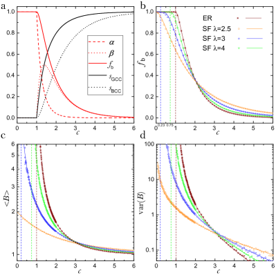
Figure 5: Bridge and bridgeness in ER and SF random networks. The size of all these random network is $10^{6}$. Curves in (a)-(d) are analytical predication about bridges, and symbols are simulation results. (a) The behavior of the bridge fraction $f_{\mathrm{b}}$, relative sizes of the BCC and GCC (denoted as $s_{\mathrm{BCC}}$, $s_{\mathrm{GCC}}$, respectively) in ER random graphs. (b) Bridge fraction in different random networks with dashed vertical lines representing the corresponding percolation threshold $c^{*}$ where the GCC and BCC emerge. Note that $c^{*}_{\mathrm{SF}}(\lambda=2.5)=0$, $c^{*}_{\mathrm{SF}}(\lambda=3.0)\approx 0.23$, $c^{*}_{\mathrm{SF}}(\lambda=4.0)\approx 0.75$, and $c^{*}_{\mathrm{ER}}=1.0$. (c) Average bridgeness in random networks. (d) The variance of bridgeness in random networks. For detailed calculation and more distributions see Supplemental Material Sec. III.

Besides $f_{\mathrm{b}}$, we can also calculate the bridgeness distribution $P(B)$ from $H_{1}(x)$. For nontrivial bridgeness ($B>0$) we only consider the bridges in the GCC. In other words, we calculate $P(B)$ for $\beta$-edges in random graphs. Define the generating function of $P(B)$ as

$$F(x)=\sum_{B=1}^{\infty}P(B)x^{B},$$

which leads to $P(B)=\frac{1}{B!}\frac{\mathrm{d}^{B}F(x)}{\mathrm{d}x^{B}}|_{x=0}.$ Since one end node of a $\beta$-edge locates in the GCC after this edge is removed (Fig. 4b), we have:

$$F(x)=\frac{2(1-u)H_{1}(x)}{\beta}=\frac{H_{1}(x)}{u},$$

where the numerator represents the generating function for the bridgeness distribution of a randomly chosen $\beta$-edge, and the denominator originates from the fact that we focus on $\beta$-edges. The moments of $P(B)$ are then given by:

$$\langle B^{k}\rangle=\sum_{B=1}^{\infty}B^{k}P(B)=\left[\left(x\frac{\mathrm{d}}{\mathrm{d}x}\right)^{k}F(x)\right]_{x=1}.$$

We calculate the average bridgeness $\langle B\rangle$ and the variance of bridgeness $\mathrm{var}(B)(:=\langle B^{2}\rangle-\langle B\rangle^{2})$ in ER and SF random networks (Fig. 5c-d). We find that for both ER and SF networks, $\langle B\rangle$ and $\mathrm{var}(B)$ monotonically decrease as $c$ increases. Note that $\langle B\rangle$ and $\mathrm{var}(B)$ of SF networks are typically lower than those of ER networks for small $c$, and higher for large $c$. This is because SF networks tend to first form densely connected components of hub nodes and then slowly stretch out. This means that they form the BCC earlier but extending bridges while ER networks absorbs bridges quickly. The divergent behavior of bridgeness around the percolation threshold $c^{*}$ is due to the emergence of the GCC, which initially is tree-like and therefore contains bridges with a huge range of bridgeness.

In conclusion, we systematically investigate the bridge structure in complex networks. We demonstrate bridges in real-world networks, calculate the fraction of bridges in different networks, and define a new edge centrality measure, called bridgeness, to quantify the importance of bridges in damaging a network. Finally we analytically calculate bridge structure in random graphs with prescribed degree distributions. The presented results help us understand the complex architecture of real-world networks and may shed lights on the design of more robust networks against bridge attack.

Acknowledgements: We thank Wei Chen for valuable discussions. This work is supported by the John Templeton Foundation (Award number 51977), National Natural Science Foundation of China (Grant No. 11505095), Research Fund for the Doctoral Program of Higher Education of China (Grant No. 20133218120033), and the Fundamental Research Funds for the Central Universities of China (Grants Nos. NS2014072 and NZ2015110). Author Contributions: Y.-Y.L conceived and designed the project. A.-K.W and L.T. did the analytical calculations. A.-K.W. did the numerical simulations and analyzed the empirical data. All authors analyzed the results. A.-K.W. and Y.-Y.L. wrote the manuscript. L.T. edited the manuscript.

Appendix A Supplemental Material

Appendix B Algorithm for identifying bridges and Calculating Bridgeness

The algorithm for identifying bridges in a network is based on depth-first search (DFS), which has linear time complexity tarjan1972depth. Randomly choosing a node from the network, we start DFS and track two indices for each node $i$: its DFS visited time stamp (DFS[$i$]) and the lowest DFS reachable ancestor (low[$i$]). $\text{DFS}[i]$ is defined as the number of other visited nodes till the current one in DFS. And $\text{low}[i]$ represents the lowest $\text{DFS}[j]$ of an previously visited node $j$ that can be reached again by current node $i$ in the later DFS. Note that, for two successively visited nodes $i$ and $j$ in the DFS, the index low[$i$] is updated by min(low[$i$], low[$j$]) after $j$ is visited.

Note that $\text{low}[i]$ marks the node’s topological position in the network. For two nodes $i$ and $j$ in the same biconnected component (BCC), low[$i$]=low[$j$]. For nodes in tree structure, low[$i$]=DFS[$i$], which is different for each node. A bridge between two nearest neighboring nodes ($i$ and $j$) is identified whenever the later visited node, say node $i$, has larger low[$i$] than that of the previously visited node $j$.

To calculate the size ($b$) of the subgraph that will be cut from the network due to the removal of a bridge, we can simply use current time step ($T$), i.e., the number of visited nodes, to subtract the DFS visited time stamp of the end of the bridge (which is inside the BCC), and plus one. For instance, in Fig. 6(c), $b=T-\text{DFS}[3]+1=6-3+1=4$. Naturally each bridge has two components to be cut from the network. And we define bridgeness to be the smaller size of the two components. Thus, to calculate the bridgeness, we need to go through the giant connected component (GCC) again, and $B$is calculated as $\text{min}\{b,S-b\}$, where $S$ represents the size of the whole connected component, see Fig. 6(e).

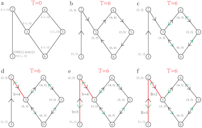
Figure 6: Using depth-first search to identify bridges and calculate bridgeness. The labels in nodes and arrows on edges represent the sequence of DFS, red edges are bridges, and for each node its two indices are presented as a coordinate (DFS[i], low[i]). (a) Initial state of indices. (b) The moment when DFS just finishes visiting all the nodes in the connected component. The size $S$ of this connected component is given by the current time step $T$. (c-e) Updates of indices when the search goes back. (f) Checking through all nodes in the component and let bridgeness be the size of the smaller part separated from that component.

To summarize, we first conduct DFS in each connected component of a graph to identify bridges with one of the separating parts ($b$) after their removal and get the size of each connected component. Then we go through the GCC again to get the bridgeness ($B$) of each $\beta$-edge.

Appendix C Previous definitions of bridgeness

The notion of bridgeness has been introduced in the literature with various different definitions. But none of them is based on the notion of bridges. Some of them are actually node-based.

C.1 A local index on edge significance in maintaining global connectivity

In cheng2010bridgeness, the bridgeness of an edge is defined to be a local index quantifying the edge importance in maintaining the network connectivity:

$$B_{e}=\frac{\sqrt{S_{x}S_{y}}}{S_{e}},$$ (1)

where $x$ and $y$ are the two endpoints of the edge $e$ and $S_{x}$, $S_{y}$, $S_{e}$ are the clique sizes of nodes $x$, $y$ and the edge $e$, respectively. A clique of size $k$ is a fully connected subgraph with $k$ nodes xiao2007empirical and the clique size of a node $x$ or an edge $e$ is defined as the size of maximum clique that contains this node or edge shen2009detect; shen2009quantifying. See Fig. 7 for a small example.

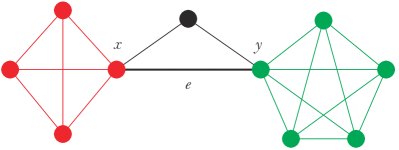
Figure 7: An example for the local bridgeness. In this example, $S_{x}=4$, $S_{y}=5$, $S_{e}=3$ and $B_{e}=1.49$.

C.2 Global bridges in networks

A node-based bridgeness, called bridgeness centrality (BRI), is derived from the node’s betweenness centrality (BC) jensen2015detecting. Consider the betweenness centrality of a node $j$ freeman1977set; freeman1979centrality:

$$BC(j)=\sum_{i\neq j\neq k}\frac{\sigma_{ik}(j)}{\sigma_{ik}},$$ (2)

where $i$, $j$, $k$ are nodes; $\sigma_{ik}$ represents the number of shortest paths between $i$ and $k$ while $\sigma_{ik}(j)$ is the number of such paths running through $j$. The bridgeness centrality of node $j$ is defined as the non-local part of its betweenness centrality:

$$BRI(j)=\sum_{i\notin N_{G}(j)\wedge k\notin N_{G}(j)}\frac{\sigma_{ik}(j)}{\sigma_{ik}},$$ (3)

where $N_{G}(j)$ are neighbor nodes of $j$. Examples are shown in Fig. 8.

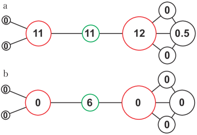
Figure 8: Betweenness centrality and bridgeness centrality. The sizes of nodes are proportional to their degrees and colored nodes are articulation points, where the green one is the global center and red ones are local centers. Numbers in nodes are their BC or BRI measures. (a) Betweenness centrality in a graph. (b) Bridgeness centrality in the same graph. Betweenness cannot differentiate the global center (the green node) from APs (red nodes), as it gives slighter higher score to high-degree nodes, which are local centers. In contrast, bridgeness centrality effectively scores the node that plays an important role in global connectivity (the green node).

C.3 Nodal bridgeness in communities with overlap

Nodal bridgeness can also be defined as a generalization of articulation point to solve the community detection problem. The number of communities $M$ in a graph can either be given in advance or by some community detection algorithm nepusz2008fuzzy and the partition of nodes is represented by the partition matrix $\textbf{U}=[u_{ik}]$, where $u_{ik}$ measures the relationship between the node $v_{k}$ and community $i$, which is determined by the complicated partition based on vertex similarities nepusz2008fuzzy. This nodal bridgeness measures the extent, to which a given node is shared among different communities nepusz2008fuzzy. If a node belongs only to one community, it has zero bridgeness while a node shared by all communities has bridgeness one. This bridgeness is defined on a vertex $v_{i}$ as the distance of its membership vector $\textbf{u}_{i}=[u_{1i},u_{2i},...,u_{Mi}]$ from the reference vector $[1/M,1/M,...1/M]$ in the Euclidean vector norm, inverted and normalized to $[0,1]$ as nepusz2008fuzzy:

$$b_{i}=1-\sqrt{\frac{M}{M-1}\sum_{j=1}^{M}\left(u_{ji}-\frac{1}{M}\right)^{2}}.$$ (4)

Appendix D Bridges in random graphs with specific degree distributions

In this section, we derive the equations in analytically calculating the first and second moments of the bridgeness distribution, as well as the relative size of GCC and BCC, for uncorrelated random graphs with prescribed degree distributions.

According to the definitions of $G_{1}(x)=\sum_{k=1}^{\infty}Q(k)x^{k-1}$, $H_{1}(x)=\sum_{k=1}^{\infty}xQ(k)[H_{1}(x)]^{k-1}$, $Q(k)=kP(k)/c$ and the self-consistency equation $H_{1}(x)=xG_{1}(H_{1}(x))$, we calculate $H_{1}^{\prime}(X)$ and $H_{1}^{\prime\prime}(x)$ as follows:

$$\begin{split}H_{1}^{\prime}(x)=G_{1}(H_{1}(x))+xG_{1}^{\prime}(H_{1}(x))H_{1}^{\prime}(x)\\ \Rightarrow H_{1}^{\prime}(x)=\frac{G_{1}(H_{1}(x))}{1-xG_{1}^{\prime}(H_{1}(x))},\end{split}$$ (5)

and

$$\begin{split}&H_{1}^{\prime\prime}(x)=\{G_{1}^{\prime}(H_{1}(x))H_{1}^{\prime}(x)[1-xG_{1}^{\prime}(H_{1}(x))]+\\ &\qquad\qquad[G_{1}^{\prime}(H_{1}(x))+xG_{1}^{\prime\prime}(H_{1}(x))H_{1}^{\prime}(x)]G_{1}(H_{1}(x))\}/\\ &\qquad\qquad[1-xG_{1}^{\prime}(H_{1}(x))]^{2}\\ &\qquad\quad=\{G_{1}^{\prime}(H_{1}(x))G_{1}(H_{1}(x))+\\ &\qquad\qquad[G_{1}^{\prime}(H_{1}(x))+xG_{1}^{\prime\prime}(H_{1}(x))H_{1}^{\prime}(x)]G_{1}(H_{1}(x))\}/\\ &\qquad\qquad[1-xG_{1}^{\prime}(H_{1}(x))]^{2}.\end{split}$$ (6)

Therefore we have:

$$\langle B\rangle=F^{\prime}(1)=\frac{H_{1}^{\prime}(1)}{u}=\frac{H_{1}^{\prime}(1)}{H_{1}(1)},$$ (7)

with $u=H_{1}(1)$ is the probability that following a randomly chosen edge to one of its end nodes, the node belongs to an FCC after removing this edge. And

$$\begin{split}&\langle B^{2}\rangle=\left[\left(x\frac{\mathrm{d}}{\mathrm{d}x}\right)^{2}F(x)\right]_{x=1}=F^{\prime}(1)+F^{\prime\prime}(1)\\ &\qquad=\frac{H_{1}^{\prime}(1)+H_{1}^{\prime\prime}(1)}{u}.\end{split}$$ (8)

Consequently, the variance of bridgeness is

$$\text{var}(B):=\langle B^{2}\rangle-\langle B\rangle^{2}=\frac{H_{1}^{\prime}(1)[u-H_{1}^{\prime}(1)]+uH_{1}^{\prime\prime}(1)}{u^{2}}.$$ (9)

Note that $G_{0}(x)=\sum_{k=0}^{\infty}P(k)x^{k}$ is the generating function of the node degree distribution $P(k)$ and $H_{0}(x)=\sum_{k=0}^{\infty}xP(k)H_{1}^{k}(x)=xG_{0}(H_{1}(x))$ is the generating function for the size distribution of components that a randomly chosen node sits in. For the calculation of the relative size of GCC, we let $s_{\text{FCC}}$ be the fraction of vertices in the graph that do not belong to the giant component. Hence we have

$$s_{\text{FCC}}=H_{0}(1)=G_{0}(u).$$ (10)

Then the relative size of the GCC is given by

$$s_{\text{GCC}}=1-s_{\text{FCC}}=1-G_{0}(u).$$ (11)

For the calculation of the relative size of BCC, it can be derived as newman100bicomponents

$$\begin{split}&s_{\text{BCC}}=1-\sum_{k=1}^{\infty}P(k)u^{k}-\sum_{k=1}^{\infty}kP(k)(1-u)u^{k-1}\\ &\qquad=1-G_{0}(u)-(1-u)G_{0}^{\prime}(u),\end{split}$$ (12)

where $\sum_{k=1}^{\infty}P(k)u^{k}+\sum_{k=1}^{\infty}kP(k)(1-u)u^{k-1}$ means that if a vertex is outside the BCC, its surroundings should have at most one element that is not $u$.

Here we propose a new method to calculate $s_{\text{BCC}}$, which relies on the result of $s_{\text{GCC}}$. Consider the $\beta$-edges, which are inside the GCC but outside of the BCC. Note that each $\beta$-edge can be assigned to one node that is inside the GCC but outside the BCC. Hence $s_{\text{BCC}}$ can be calculated as:

$$s_{\text{BCC}}=s_{\text{GCC}}-\beta c/2=s_{\text{GCC}}-u(1-u)c,$$ (13)

where $\beta c/2=u(1-u)c$ represents the fraction of $\beta$-edges normalized by total number of nodes. Note that the above two equations are equivalent, because $G_{0}^{\prime}(u)=cG_{1}(u)=cu$.

D.1 Poisson-distributed graphs

The degree distribution $P(k)$ for Erdős-Rényi random graphs follows Poisson distribution erdos1960evolution:

$$P(k)=\frac{e^{-c}c^{k}}{k!},$$ (14)

with $c$ is the mean degree. Then the generating functions are:

$$G_{0}(x,c)=e^{c(x-1)},$$ (15)

$$G_{1}(x,c)=e^{c(x-1)},$$ (16)

with derivatives:

$$G_{1}^{\prime}(x)=ce^{c(x-1)},$$ (17)

$$G_{1}^{\prime\prime}(x)=c^{2}e^{c(x-1)}.$$ (18)

With

$$u=H_{1}(1)=G_{1}(H_{1}(1))=e^{c(u-1)},$$ (19)

and

$$H_{1}^{\prime}(1)=\frac{G_{1}(u)}{1-G_{1}^{\prime}(u)}=\frac{u}{1-cu},$$ (20)

we have

$$f_{\text{b}}=[1-(1-u)^{2}],$$ (21)

and

$$\langle B\rangle=\frac{1}{1-cu}.$$ (22)

Substituting Eq. (S16-22) into Eq. (S6-9), we can get

$$\text{var}(B)=\frac{cu}{(1-cu)^{3}}.$$ (23)

Besides, by Eq. (S11-13, 19), we also have

$$s_{\text{GCC}}=1-e^{c(u-1)},$$ (24)

and

$$s_{\text{BCC}}=1-e^{c(u-1)}-u(1-u)c.$$ (25)

Results are shown in main text Fig. 5.

D.2 Exponentially distributed graphs

The degree distribution for exponentially distributed graphs is liu2012core; newman2001random :

$$P(k)=(1-e^{-1/\kappa})e^{-k/\kappa},$$ (26)

and the mean degree is

$$c=\frac{e^{-1/\kappa}}{1-e^{-1/\kappa}}.$$ (27)

The generating functions are

$$G_{0}(x)=\frac{1-e^{-1/\kappa}}{1-xe^{-1/\kappa}},$$ (28)

$$G_{1}(x)=\left[\frac{1-e^{-1/\kappa}}{1-xe^{-1/\kappa}}\right]^{2},$$ (29)

with derivatives

$$G_{1}^{\prime}(x)=\frac{2e^{-1/\kappa}(1-e^{-1/\kappa})^{2}}{(1-xe^{-1/\kappa})^{3}},$$ (30)

$$G_{1}^{\prime\prime}(x)=\frac{6e^{-2/\kappa}(1-e^{-1/\kappa})^{2}}{(1-xe^{-1/\kappa})^{4}}.$$ (31)

Inserting Eq. (S26-31) into Eq. (S5-13), we can get $f_{\text{b}}$, $s_{\text{GCC}}$, $s_{\text{BCC}}$, $\langle B\rangle$ and $\text{var}(B)$. Results of these quantities can be found in Fig. 9,10.

D.3 Purely power-law distributed graphs

The degree distribution for purely power-law distributed graphs is liu2012core; newman2001random:

$$P(k)=\frac{k^{-\lambda}}{\zeta(\lambda)}\qquad\text{for}\qquad k\geq 1,$$ (32)

where $\zeta(\lambda)=\sum_{k=1}^{\infty}k^{-\lambda}$ is the Riemann Zeta function. Note that $P(k)$ can be normalized only for $\lambda\geq 2$. It is obvious that the mean degree is larger than $1$ in this situation and larger $\lambda$ leads to smaller mean degree.

The generating functions are

$$G_{0}(x)=\frac{\text{Li}_{\lambda}(x)}{\zeta(\lambda)},$$ (33)

$$G_{1}(x)=\frac{\text{Li}_{\lambda-1}(x)}{x\zeta(\lambda-1)},$$ (34)

where $\text{Li}_{n}(x)=\sum_{k=1}^{\infty}x^{k}/k^{n}$ is the $n$th polylogarithm of $x$, whose derivative is $\frac{\mathrm{d}\text{Li}_{n}(x)}{\mathrm{d}x}=\frac{\text{Li}_{\lambda-1}(x)}{x}$. The derivatives of the generating functions are

$$G_{1}^{\prime}(x)=\frac{\text{Li}_{\lambda-2}(x)-\text{Li}_{\lambda-1}(x)}{x^{2}\zeta(\lambda-1)},$$ (35)

$$G_{1}^{\prime\prime}(x)=\frac{\text{Li}_{\lambda-3}(x)-3\text{Li}_{\lambda-2}(x)+2\text{Li}_{\lambda-1}(x)}{x^{3}\zeta(\lambda-1)}.$$ (36)

Inserting Eq. (S32-36) into Eq. (S5-13), we can get $f_{\text{b}}$, $s_{\text{GCC}}$, $s_{\text{BCC}}$, $\langle B\rangle$ and $\text{var}(B)$. Results are shown in Fig. 9,10.

D.4 Power-law distribution with exponential cutoff

The degree distribution for a purely power-law distribution with exponent $\lambda$ and exponential cutoff is liu2012core; newman2001random:

$$P(k)=\frac{k^{-\lambda}e^{-k/\kappa}}{\text{Li}_{\lambda}(e^{-1/\kappa})}\qquad\text{for}\qquad k\geq 1.$$ (37)

This distribution can be normalized for any $\lambda$.

The generating functions are

$$G_{0}(x)=\frac{\text{Li}_{\lambda}(xe^{-1/\kappa})}{\text{Li}_{\lambda}(e^{-1/\kappa})}.$$ (38)

$$G_{1}(x)=\frac{\text{Li}_{\lambda-1}(xe^{-1/\kappa})}{x\text{Li}_{\lambda-1}(e^{-1/\kappa})},$$ (39)

$$G_{1}^{\prime}(x)=\frac{\text{Li}_{\lambda-2}(xe^{-1/\kappa})-\text{Li}_{\lambda-1}(xe^{-1/\kappa})}{x^{2}\text{Li}_{\lambda-1}(e^{-1/\kappa})}.$$ (40)

$$G_{1}^{\prime\prime}(x)=\frac{\text{Li}_{\lambda-3}(xe^{-1/\kappa})-3\text{Li}_{\lambda-2}(xe^{-1/\kappa})+2\text{Li}_{\lambda-1}(xe^{-1/\kappa})}{x^{3}\text{Li}_{\lambda-1}(e^{-1/\kappa})}.$$ (41)

Inserting Eq. (S37-41) into Eq. (S5-13), we can get $f_{\text{b}}$, $s_{\text{GCC}}$, $s_{\text{BCC}}$, $\langle B\rangle$ and $\text{var}(B)$. Results are shown in Fig. 9,10.

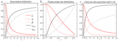
Figure 9: The analytical results of the bridge fraction $f_{\text{b}}$, relative sizes of the BCC and GCC in different random graphs. (a) Exponentially distributed graphs. (b) Purely power-law distributed graphs. (c) Power-law distribution with exponential cutoff parameter $\kappa=100$.

Figure 10: Bridge fraction, average and variance of bridgeness in different degree distribution. All the results are analytical and the dashed lines mark their percolation positions.

D.5 Static model

In the main text, we use static model to generate scale-free (SF) random graphs goh2001universal. This model consists of following steps liu2012core:

• Given $N$ isolated nodes, we label them from $1$ to $N$. For each node i, we assign a weight $p_{i}\propto i^{-a}$, where $a=\frac{1}{\lambda-1}$ and $\lambda$ is the characteristic parameter of SF graphs.

• Then we randomly choose two nodes according to their weights and connect them if they are not connected. Self-links and multi-links are forbidden here. We repeat this step until $M=cN/2$ links are added.

The degree distribution of the static mode can be analytically derived as catanzaro2005analytic; lee2006intrinsic:

$$P(k)=\frac{[c(1-a)]^{1/a}}{a}\frac{\Gamma(k-1/a,c(1-a))}{\Gamma(k+1)},$$ (42)

with $\Gamma(s)$ the gamma function and $\Gamma(s.x)$ the upper incomplete gamma function. When $k\to\infty$, $P(k)\sim k^{-(1+1/a)}=k^{-\lambda}$. Therefore, we can build different SF random graphs by tuning $a$. The generating functions are:

$$G_{0}(x)=\frac{1}{a}E_{1+\frac{1}{a}}[c(1-a)(1-x)],$$ (43)

$$G_{1}(x)=\frac{1-a}{a}E_{\frac{1}{a}}[c(1-a)(1-x)],$$ (44)

where $E_{n}=\int_{1}^{\infty}e^{-xy}y^{-n}\mathrm{d}y$ is the exponential integral. Note that the derivative of $E_{n}$ follows $E_{n}^{\prime}=-E_{n-1}(x)$. From the generating functions, we can derive $f_{\text{b}}$, $s_{\text{GCC}}$, $s_{\text{BCC}}$, $\langle B\rangle$ and $\text{var}(B)$. Results are shown in main text Fig. 5.

Appendix E Network datasets

Detailed information about the real-world networks analyzed in this paper are listed in Tables S1 with brief descriptions. We categorize networks according to their types and show their names, numbers of nodes, edges, bridges and biconnected components, size of the GCC as well as the average, variance and maximum of bridgeness.

Table 1: Real network datasets.

category	name	$N$	$L$	$s_{\text{GCC}}$	$N_{\text{BCC}}$	$N_{\text{bridges}}$	$\langle B\rangle$	$\text{var}(B)$	$B_{\text{max}}$	description
Air traffic	USairport500 colizza2007reaction	500	2,980	500	4	82	1.15	0.37	5	Network among the top 500 busiest
										commercial airports in US
	USairport-2010 opsahl2011anchorage	1,574	17,215	1,572	1	335	1.02	0.023	2	US airport network in 2010
	openfights opsahl2011anchorage	2,939	15,677	2,905	6	724	1.15	0.89	20	non-US-based airport network
Road networks leskovec2015snap	RoadNet-CA	1,965,206	2,766,607	1,957,027	4,042	376,517	1.598	6.53	162	California road network
	RoadNet-PA	1,088,092	1,541,898	1,087,562	1,815	216,994	1.39	2.16	94	Pennsylvania road network
	RoadNet-TX	1,379,917	1,921,660	1,351,137	3,054	290,333	1.48	5.32	209	Texas road network
Power grids (PG)	PG-Texas bianconi2008local	4889	5855	4889	3	1425	1.40	1.61	27	Power grid in Texas
	PG-WestState watts1998collective	4,941	6,594	4,941	16	1,611	1.58	2.37	18	High-voltage power grid in the Western
										states in US
Internet:	as20000102	6,474	12,572	6,474	1	2,451	1.04	0.064	5	AS graph from January 02, 2000
Autonomous	oregon1-010331	10,670	22,002	10,670	1	3,799	1.03	0.077	10	AS peering information inferred from
										Oregon route-views (I)
Systems(AS) leskovec2015snap	oregon1-010407	10,729	21,999	10,729	1	3,848	1.03	0.048	5	Same as above (at different time)
	oregon1-010414	10,790	22,469	10,790	1	3,853	1.03	0.048	5	Same as above (at different time)
	oregon1-010421	10,859	22,747	10,859	1	3,855	1.03	0.047	6	Same as above (at different time)
	oregon1-010428	10,886	22,493	10,886	1	3,844	1.03	0.049	7	Same as above (at different time)
	oregon1-010505	10,943	22,607	10,943	1	3,832	1.03	0.046	6	Same as above (at different time)

category	name	$N$	$L$	$s_{\text{GCC}}$	$N_{\text{BCC}}$	$N_{\text{bridges}}$	$\langle B\rangle$	$\text{var}(B)$	$B_{\text{max}}$	description
Internet:	oregon1-010512	11,011	22,677	11,011	1	3,909	1.03	0.047	7	Same as above (at different time)
Autonomous	oregon1-010519	11,051	22,724	11,051	1	3,920	1.03	0.044	6	Same as above (at different time)
Systems(AS) leskovec2015snap	oregon1-010526	11,174	23,409	11,174	1	3,946	1.02	0.035	6	Same as above (at different time)
	oregon2-010331	10,900	31,180	10,900	1	3,274	1.02	0.025	6	AS peering information inferred from Oregon
										route-views (II)
	oregon2-010407	10,981	30,855	10,981	1	3,332	1.02	0.032	5	Same as above (at different time)
	oregon2-010414	11,019	31,761	11,019	1	3,316	1.014	0.019	4	Same as above (at different time)
	oregon2-010421	11,080	31,538	11,080	1	3,294	1.015	0.022	5	Same as above (at different time)
	oregon2-010428	11,113	31,434	11,113	1	3,283	1.016	0.020	3	Same as above (at different time)
	oregon2-010505	11,157	30,943	11,157	1	3,282	1.014	0.017	3	Same as above (at different time)
	oregon2-010512	11,260	31,303	11,260	2	3,296	1.017	0.026	5	Same as above (at different time)
	oregon2-010519	11,375	32,287	11,375	1	3,320	1.016	0.019	3	Same as above (at different time)
	oregon2-010526	11,461	32,730	11,461	1	3,351	1.015	0.018	4	Same as above (at different time)
Electronic	s838	512	819	512	1	49	1.33	0.22	2	Electronic sequential logic circuit
circuits milo2002network	s420	252	399	252	1	25	1.32	0.22	1	Same as above
	s208	122	189	122	1	13	1.31	0.21	2	Same as above
World Wide Web	stanford.edu leskovec2015snap	281,903	1,992,636	255,265	1,073	27,344	4.42	2,081.1	4907	WWW from stanford.edu domain
(WWW)	nd.edu albert1999internet	325,729	1,090,108	325,729	308	166,376	1.58	264.29	2,660	WWW from nd.edu domain
Neural network watts1998collective	C.elegans	297	2,148	297	1	15	1.00	0.00	0	Neural network of C.elegans

category	name	$N$	$L$	$s_{\text{GCC}}$	$N_{\text{BCC}}$	$N_{\text{bridges}}$	$\langle B\rangle$	$\text{var}(B)$	$B_{\text{max}}$	description
Inertnet:	p2p-Gnutella04	10,876	39,994	10,876	1	2,497	1.020	0.099	12	Gnutella p2p file sharing network
peer-to-peer (p2p)	p2p-Gnutella05	8,846	31,839	8,842	1	2,009	1.011	0.012	3	Same as above (at different time)
(p2p)file sharing	p2p-Gnutella06	8,717	31,525	8,717	1	1,990	1.012	0.013	3	Same as above (at different time)
file sharing networks leskovec2015snap	p2p-Gnutella08	6,301	20,777	6,299	1	1,765	1.016	0.067	10	Same as above (at different time)
	p2p-Gnutella09	8,114	26,013	8,104	1	2,503	1.008	0.010	2	Same as above (at different time)
	p2p-Gnutella24	26,518	65,369	26,498	1	10,989	1.005	0.0053	2	Same as above (at different time)
	p2p-Gnutella25	22,687	54,705	22,663	1	9,322	1.006	0.014	9	Same as above (at different time)
	p2p-Gnutella30	36,682	88,328	36,646	1	16,477	1.004	0.005	3	Same as above (at different time)
	p2p-Gnutella31	62,586	147,892	62,561	1	28,759	1.005	0.0075	6	Same as above (at different time)
Food webs (FW)	baydry ulanowicz1998fy97	128	2,106	128	1	0	0.00	0.00	0	FW at Florida Bay, Dry Season
	baywet ulanowicz1998fy97	128	2,075	128	1	0	0.00	0.00	0	FW at Florida Bay, Wet Season
	Chesapeake baird1989seasonal	39	170	39	1	0	0.00	0.00	0	FW at Chesapeake Bay Mesohaline Net
	ChesLower hagy2002eutrophication	37	167	37	1	0	0.00	0.00	0	FW at Lower Chesapeake Bay in Summer
	ChesMiddle hagy2002eutrophication	37	198	37	1	0	0.00	0.00	0	FW at Middle Chesapeake Bay in Summer
	ChesUpper hagy2002eutrophication	37	199	37	1	0	0.00	0.00	0	FW at Upper Chesapeake Bay in Summer
	CrystalC ulanowicz2012growth	24	114	24	1	0	0.00	0.00	0	FW at Crystal River Creek (Control)
	CrystalD ulanowicz2012growth	24	92	24	1	0	0.00	0.00	0	FW at Crystal River Creek (Delta Temp)
	cypdry websitepajek	71	618	71	1	0	0.00	0.00	0	FW at Cypress, Dry Season
	cypwet websitepajek	71	612	71	1	0	0.00	0.00	0	FW at Cypress, Wet Season

category	name	$N$	$L$	$s_{\text{GCC}}$	$N_{\text{BCC}}$	$N_{\text{bridges}}$	$\langle B\rangle$	$\text{var}(B)$	$B_{\text{max}}$	description
Food webs (FW)	Everglades ulanowicz2000annual	69	880	69	1	0	0.00	0.00	0	FW at Everglades Graminoid Marshes
	Florida ulanowicz1998fy97	128	2,075	128	1	0	0.00	0.00	0	FW at Florida Bay Trophic Exchange Matrix
	gramdry ulanowicz2000annual	69	879	69	1	0	0.00	0.00	0	FW at Everglades Graminoids, Dry Season
	gramwet ulanowicz2000annual	69	880	69	1	0	0.00	0.00	0	FW at Everglades Graminoids, Wet Season
	grassland dunne2002two	88	137	88	4	30	1.80	2.69	5	FW at Grassland
	littlerock martinez1991artifacts	183	2,434	183	1	1	1.00	0.00	0	FW at Little Rock lake.
	mangdry patricio2005thesis	97	1,445	97	1	0	0.00	0.00	0	FW at Mangrove Estuary, Dry Season
	mangwet patricio2005thesis	97	1,446	97	1	0	0.00	0.00	0	FW at Mangrove Estuary, Wet Season
	Maspalomas almunia1999benthic	24	77	24	1	0	0.00	0.00	0	FW at Charca de Maspalomas
	Michigan websitepajek	39	209	39	1	0	0.00	0.00	0	FW at Lake Michigan Control network
	Mondego patricio2005thesis	46	358	46	1	1	1.00	0.00	0	FW at Mondego Estuary - Zostrea site
	Narragan patricio2005thesis	35	204	35	1	0	0.00	0.00	0	FW at Narragansett Bay Model
	Rhode websitepajek	20	45	19	1	0	0.00	0.00	0	FW at Rhode River Watershed - Water Budget
	seagrass christian1999organizing	49	223	49	1	0	0.00	0.00	0	FW at St. Marks Seagrass.
	silwood memmott2000predators	154	365	153	1	60	1.20	0.56	4	FW at Silwood Park
	StMarks baird1998assessment	54	350	54	1	0	0.00	0.00	0	FW at St. Marks River (Florida) Flow network
	stmartin goldwasser1993construction	45	224	45	1	2	1.00	0.00	1	FW at St. Martin Island
	ythan dunne2002two	135	596	135	1	7	1.00	0.00	1	FW at Ythan Estuary

category	name	$N$	$L$	$s_{\text{GCC}}$	$N_{\text{BCC}}$	$N_{\text{bridges}}$	$\langle B\rangle$	$\text{var}(B)$	$B_{\text{max}}$	description
Transcriptional	TRN-Yeast-Babu balaji2006comprehensive	4,441	12,864	4,441	1	1,556	1.00	0.00	0	Transcriptional regulatory network
										of S.cerevisiae
regulatory networks	TRN-Yeast-Alon milo2002network	688	1,078	662	1	343	1.31	3.17	20	Same as above (compiled by different
										group)
(TRN)	TRN-EC-RDB64 gama2008regulondb	1,550	3,234	1,454	1	616	1.046	0.18	7	Transcriptional regulatory network
										of E.coli
	TRN-EC-Alon milo2002network	418	519	328	3	251	1.45	5.86	24	Same as above (compiled by different
										group)
Communication	Cellphone song2010limits	36,595	56,853	30,420	415	13,382	1.66	2.56	36	Call network of cell phone users
networks	Email-Enron leskovec2015snap	36,692	183,831	33,696	366	10,714	1.08	1.53	105	Email communication network from
										Enron
	Email-EuAll leskovec2015snap	265,214	364,481	224,832	10	213,190	1.012	0.52	169	Email network from a large European
										research institute
	Email-epoch eckmann2004entropy	3,188	31,857	3,186	1	613	1.0016	0.0016	1	Email network in a university
	UCIonline opsahl2009clustering	1,899	13,838	1,893	1	398	1.020	0.025	2	Online message network of students
										at UC, Irvine
	WikiTalk leskovec2015snap	2,394,385	4,659,565	2,388,953	13	1,768,844	1.0024	0.0043	19	Wikipedia talk network
Social networks	Epinions richardson2003semantic	75,888	405,740	75,877	87	38,679	1.12	0.35	34	Who-trusts-whom network of
										Epinions.com

category	name	$N$	$L$	$s_{\text{GCC}}$	$N_{\text{BCC}}$	$N_{\text{bridges}}$	$\langle B\rangle$	$\text{var}(B)$	$B_{\text{max}}$	description
Social networks	college student van2003evolution; milo2004superfamilies	32	80	32	1	0	0.00	0.00	0	Social networks of positive sentiment
	prison inmate van2003evolution; milo2004superfamilies	67	142	67	1	5	1.20	0.16	1	Same as above (prison inmates)
	Slashdot-1 leskovec2015snap	77,357	468,554	77,350	46	29,680	1.063	0.096	8	Slashdot social network
	Slashdot-2 leskovec2015snap	81,871	497,672	81,867	46	29,998	1.066	0.1084	9	Same as above (at different time)
	Slashdot-3 leskovec2015snap	82,144	500,481	82,140	46	30,086	1.066	0.1084	8	Same as above (at different time)
	Slashdot-4 leskovec2015snap	77,360	469,180	77,360	46	29,649	1.063	0.096	9	Same as above (at different time)
	Slashdot-5 leskovec2015snap	82,168	504,230	82,168	45	30,035	1.066	0.108	8	Same as above (at different time)
	Twitter leskovec2015snap	81,306	1,342,296	81,306	1	4,996	1.00	0.00	0	Social circles from Twitter
	WikiVote leskovec2015snap	7,115	100,762	7,066	1	2,306	1.006	0.011	5	Wikipedia who-votes-on-whom network
	Youtube leskovec2015snap	1,134,890	2,987,624	1,134,890	1,944	667,090	1.20	1.25	91	Youtube online social network
Intra-	Freemans-1 freeman1979networkers	34	415	34	1	0	0.00	0.00	0	Social network of network researchers
organizational	Freemans-2 freeman1979networkers	34	474	34	1	0	0.00	0.00	0	Same as above (at different time)
networks	Freemans-3 freeman1979networkers	32	266	32	1	0	0.00	0.00	0	Same as above (at different time)
	Consulting-1 cross2004hidden	46	550	46	1	0	0.00	0.00	0	Social network from a consulting company
	Consulting-2 cross2004hidden	46	505	46	1	0	0.00	0.00	0	Same as above (different evaluation)
	Manufacturing-1 cross2004hidden	77	1,344	77	1	0	0.00	0.00	0	Social network from a manufacturing
										company
	Manufacturing-2 cross2004hidden	77	1,341	77	1	0	0.00	0.00	0	Same as above (different evaluation)
PPI networks	CCSB-Y2H yu2008high	892	1,015	787	1	627	1.145	0.197	4	Interactions from CCSB-YI11

category	name	$N$	$L$	$s_{\text{GCC}}$	$N_{\text{BCC}}$	$N_{\text{bridges}}$	$\langle B\rangle$	$\text{var}(B)$	$B_{\text{max}}$	description
PPI networks	Y2H-union yu2008high	1,304	1,412	946	1	820	1.48	1.36	12	The union of CCSB-YI1, Ito-core and
										Uetz-screen
	wi2004 simonis2009empirically	743	827	511	1	477	1.37	0.91	9	Interactions from 2004 Y2H screen
	wi2007 simonis2009empirically	814	863	545	1	522	1.40	0.97	8	Interactions from 2007 Y2H screen
	HI-I-05 rual2005towards	1,551	2,612	1,307	2	803	1.20	0.41	8	Proteome-scale map of the human binary interactome
										network generated by systematically screening Space-I
	HI-II-14 rolland2014proteome	4,305	13,428	4,100	1	1,652	1.08	0.13	4	Same as above (by different screening space)

References

- Bollobás (1998) B. Bollobás, Modern graph theory, volume 184 of Graduate Texts in Mathematics (Springer-Verlag, New York, 1998).
- Behzad and Chartrand (1972) M. Behzad and G. Chartrand, Introduction to the Theory of Graphs (Allyn and Bacon, Boston, 1972).
- Harary et al. (1969) F. Harary et al., Graph theory (Addison-Wesley Reading, MA, 1969).
- Tarjan (1972) R. Tarjan, SIAM Journal on Computing 1, 146 (1972).
- (5) L. Tian, A. Bashan, D.-N. Shi, and Y.-Y. Liu, Nat. Commun. (in press), arXiv:1609.00094 .
- Pike and Stanley (1981) R. Pike and H. E. Stanley, J. Phys. A: Math. Gen. 14, L169 (1981).
- Dunne et al. (2002) J. A. Dunne, R. J. Williams, and N. D. Martinez, Proc. Natl. Acad. Sci. USA 99, 12917 (2002).
- Simonis et al. (2009) N. Simonis, J.-F. Rual, A.-R. Carvunis, M. Tasan, I. Lemmens, T. Hirozane-Kishikawa, T. Hao, J. M. Sahalie, K. Venkatesan, F. Gebreab, et al., Nat. Methods 6, 47 (2009).
- Leskovec and Krevl (2014) J. Leskovec and A. Krevl, SNAP Datasets: Stanford Large Network Dataset Collection (https://snap.stanford.edu/data/) (2014).
- Watts and Strogatz (1998) D. J. Watts and S. H. Strogatz, nature 393, 440 (1998).
- Erdös and Rényi (1960) P. Erdös and A. Rényi, Publ. Math. Inst. Hung. Acad. Sci 5, 43 (1960).
- Bollobás et al. (2001) B. Bollobás, W. Fulton, A. Katok, F. Kirwan, and P. Sarnak, in Random graphs (Cambridge University Press, New York, 2001).
- Nepusz et al. (2008) T. Nepusz, A. Petróczi, L. Négyessy, and F. Bazsó, Phys. Rev. E 77, 016107 (2008).
- Gong et al. (2011) K. Gong, M. Tang, H. Yang, and M. Shang, Chaos 21, 043130 (2011).
- Jensen et al. (2015) P. Jensen, M. Morini, M. Karsai, T. Venturini, A. Vespignani, M. Jacomy, J.-P. Cointet, P. Mercklé, and E. Fleury, Journal of Complex Networks , cnv022 (2015).
- Cheng et al. (2010) X.-Q. Cheng, F.-X. Ren, H.-W. Shen, Z.-K. Zhang, and T. Zhou, J. Stat. Mech. 2010, P10011 (2010).
- Newman and Ghoshal (2008) M. E. J. Newman and G. Ghoshal, Phys. Rev. Lett. 100, 1 (2008).
- Newman et al. (2001) M. E. Newman, S. H. Strogatz, and D. J. Watts, Phys. Rev. E 64, 026118 (2001).
- Cohen et al. (2000) R. Cohen, K. Erez, D. Ben-Avraham, and S. Havlin, Phys. Rev. Lett. 85, 4626 (2000).
- Callaway et al. (2000) D. S. Callaway, M. E. Newman, S. H. Strogatz, and D. J. Watts, Phys. Rev. Lett. 85, 5468 (2000).
- Dorogovtsev et al. (2008) S. N. Dorogovtsev, A. V. Goltsev, and J. F. Mendes, Rev. Mod. Phys. 80, 1275 (2008).
- Mezard and Montanari (2009) M. Mezard and A. Montanari, Information, physics, and computation (Oxford University Press, 2009).
- Goh et al. (2001) K.-I. Goh, B. Kahng, and D. Kim, Phys. Rev. Lett. 87, 278701 (2001).
- Catanzaro and Pastor-Satorras (2005) M. Catanzaro and R. Pastor-Satorras, Eur. Phys. J. B 44, 241 (2005).
- Lee et al. (2006) J.-S. Lee, K.-I. Goh, B. Kahng, and D. Kim, Eur. Phys. J. B 49, 231 (2006).

References

- Tarjan (1972) R. Tarjan, SIAM Journal on Computing 1, 146 (1972).
- Cheng et al. (2010) X.-Q. Cheng, F.-X. Ren, H.-W. Shen, Z.-K. Zhang, and T. Zhou, J. Stat. Mech. 2010, P10011 (2010).
- Xiao et al. (2007) W.-K. Xiao, J. Ren, F. Qi, Z.-W. Song, M.-X. Zhu, H.-F. Yang, H.-Y. Jin, B.-H. Wang, and T. Zhou, Phys. Rev. E 76, 037102 (2007).
- Shen et al. (2009a) H. Shen, X. Cheng, K. Cai, and M.-B. Hu, Physica A 388, 1706 (2009a).
- Shen et al. (2009b) H.-W. Shen, X.-Q. Cheng, and J.-F. Guo, J. Stat. Mech. 2009, P07042 (2009b).
- Jensen et al. (2015) P. Jensen, M. Morini, M. Karsai, T. Venturini, A. Vespignani, M. Jacomy, J.-P. Cointet, P. Mercklé, and E. Fleury, Journal of Complex Networks , cnv022 (2015).
- Freeman (1977) L. C. Freeman, Sociometry , 35 (1977).
- Freeman et al. (1979) L. C. Freeman et al., Social networks 1, 215 (1979).
- Nepusz et al. (2008) T. Nepusz, A. Petróczi, L. Négyessy, and F. Bazsó, Phys. Rev. E 77, 016107 (2008).
- (10) M. Newman and G. Ghoshal, Phys. Rev. Lett 100, 138701.
- Erdös and Rényi (1960) P. Erdös and A. Rényi, Publ. Math. Inst. Hung. Acad. Sci 5, 43 (1960).
- Liu et al. (2012) Y.-Y. Liu, E. Csóka, H. Zhou, and M. Pósfai, Phys. Rev. Lett. 109, 205703 (2012).
- Newman et al. (2001) M. E. Newman, S. H. Strogatz, and D. J. Watts, Phys. Rev. E 64, 026118 (2001).
- Goh et al. (2001) K.-I. Goh, B. Kahng, and D. Kim, Phys. Rev. Lett. 87, 278701 (2001).
- Catanzaro and Pastor-Satorras (2005) M. Catanzaro and R. Pastor-Satorras, Eur. Phys. J. B 44, 241 (2005).
- Lee et al. (2006) J.-S. Lee, K.-I. Goh, B. Kahng, and D. Kim, Eur. Phys. J. B 49, 231 (2006).
- Colizza et al. (2007) V. Colizza, R. Pastor-Satorras, and A. Vespignani, Nat. Phys. 3, 276 (2007).
- Opsahl (2011) T. Opsahl, Why anchorage is not (that) important: Binary ties and sample selection (http://toreopsahl.com/2011/08/12/why-anchorage-is-not-that-important-binary-tiesand-sample-selection) (2011).
- Leskovec and Krevl (2014) J. Leskovec and A. Krevl, SNAP Datasets: Stanford Large Network Dataset Collection (https://snap.stanford.edu/data/) (2014).
- Bianconi et al. (2008) G. Bianconi, N. Gulbahce, and A. E. Motter, Phys. Rev. Lett. 100, 118701 (2008).
- Watts and Strogatz (1998) D. J. Watts and S. H. Strogatz, nature 393, 440 (1998).
- Milo et al. (2002) R. Milo, S. Shen-Orr, S. Itzkovitz, N. Kashtan, D. Chklovskii, and U. Alon, Science 298, 824 (2002).
- Albert et al. (1999) R. Albert, H. Jeong, and A.-L. Barabási, Nature 401, 130 (1999).
- (24) R. E. Ulanowicz and D. L. DeAngelis, FY97: The Florida Bay Ecosystem pp. 20688-20038 (1998) .
- Baird and Ulanowicz (1989) D. Baird and R. E. Ulanowicz, Ecological monographs 59, 329 (1989).
- Hagy (2002) J. D. Hagy, Eutrophication, hypoxia and trophic transfer efficiency in Chesapeake Bay (PhD Dissertation, University of Maryland at College Park (USA), 446 pp, 2002).
- Ulanowicz (2012) R. E. Ulanowicz, Growth and development: ecosystems phenomenology (Springer Science & Business Media, 2012).
- (28) Pajek food web datasets, http://vlado.fmf.uni-lj.si/pub/networks/data/bio/foodweb/foodweb.htm .
- Ulanowicz et al. (2000) R. E. Ulanowicz, J. J. Heymans, and M. S. Egnotovich, Annual Report to the United States Geological Service Biological Resources Division Ref. No.[UMCES] CBL 00-0176, Chesapeake Biological Laboratory, University of Maryland (2000).
- Dunne et al. (2002) J. A. Dunne, R. J. Williams, and N. D. Martinez, Proc. Nat. Acad. Sci. 99, 12913 (2002).
- Martinez (1991) N. D. Martinez, Ecological Monographs 61, 367 (1991).
- Patrcio (2005) J. M. Patrcio, PhD thesis, University of Coimbra, Coimbra, Portugal (2005).
- Almunia et al. (1999) J. Almunia, G. Basterretxea, J. Arıstegui, and R. Ulanowicz, Estuarine, Coastal and Shelf Science 49, 363 (1999).
- Christian and Luczkovich (1999) R. R. Christian and J. J. Luczkovich, Ecological Modelling 117, 99 (1999).
- Memmott et al. (2000) J. Memmott, N. D. Martinez, and J. Cohen, Journal of Animal Ecology 69, 1 (2000).
- Baird et al. (1998) D. Baird, J. Luczkovich, and R. R. Christian, Estuarine, Coastal and Shelf Science 47, 329 (1998).
- Goldwasser and Roughgarden (1993) L. Goldwasser and J. Roughgarden, Ecology 74, 1216 (1993).
- Balaji et al. (2006) S. Balaji, M. M. Babu, L. M. Iyer, N. M. Luscombe, and L. Aravind, Journal of molecular biology 360, 213 (2006).
- Gama-Castro et al. (2008) S. Gama-Castro, V. Jiménez-Jacinto, M. Peralta-Gil, A. Santos-Zavaleta, M. I. Peñaloza-Spinola, B. Contreras-Moreira, J. Segura-Salazar, L. Muñiz-Rascado, I. Martínez-Flores, H. Salgado, et al., Nucleic acids research 36, D120 (2008).
- Song et al. (2010) C. Song, Z. Qu, N. Blumm, and A.-L. Barabási, Science 327, 1018 (2010).
- Eckmann et al. (2004) J.-P. Eckmann, E. Moses, and D. Sergi, Proc. Nat. Acad. Sci. 101, 14333 (2004).
- Opsahl and Panzarasa (2009) T. Opsahl and P. Panzarasa, Social networks 31, 155 (2009).
- Richardson et al. (2003) M. Richardson, R. Agrawal, and P. Domingos, The Semantic Web-ISWC 2003 (Springer, 2003).
- Van Duijn et al. (2003) M. A. Van Duijn, E. P. Zeggelink, M. Huisman, F. N. Stokman, and F. W. Wasseur, Journal of Mathematical Sociology 27, 153 (2003).
- Milo et al. (2004) R. Milo, S. Itzkovitz, N. Kashtan, R. Levitt, S. Shen-Orr, I. Ayzenshtat, M. Sheffer, and U. Alon, Science 303, 1538 (2004).
- Freeman and Freeman (1979) S. C. Freeman and L. C. Freeman, The networkers network: A study of the impact of a new communications medium on sociometric structure (School of Social Sciences University of Calif., 1979).
- Cross and Parker (2004) R. L. Cross and A. Parker, The hidden power of social networks: Understanding how work really gets done in organizations (Harvard Business Review Press, 2004).
- Yu et al. (2008) H. Yu, P. Braun, M. A. Yıldırım, I. Lemmens, K. Venkatesan, J. Sahalie, T. Hirozane-Kishikawa, F. Gebreab, N. Li, N. Simonis, et al., Science 322, 104 (2008).
- Simonis et al. (2009) N. Simonis, J.-F. Rual, A.-R. Carvunis, M. Tasan, I. Lemmens, T. Hirozane-Kishikawa, T. Hao, J. M. Sahalie, K. Venkatesan, F. Gebreab, et al., Nat. Methods 6, 47 (2009).
- Rual et al. (2005) J.-F. Rual, K. Venkatesan, T. Hao, T. Hirozane-Kishikawa, A. Dricot, N. Li, G. F. Berriz, F. D. Gibbons, M. Dreze, N. Ayivi-Guedehoussou, et al., Nature 437, 1173 (2005).
- Rolland et al. (2014) T. Rolland, M. Taşan, B. Charloteaux, S. J. Pevzner, Q. Zhong, N. Sahni, S. Yi, I. Lemmens, C. Fontanillo, R. Mosca, et al., Cell 159, 1212 (2014).