Combining Data-driven and Model-driven Methods for Robust Facial Landmark Detection

Abstract

Facial landmark detection is an important yet challenging task for real-world computer vision applications. This paper proposes an effective and robust approach for facial landmark detection by combining data- and model-driven methods. Firstly, a Fully Convolutional Network (FCN) is trained to compute response maps of all facial landmark points. Such a data-driven method could make full use of holistic information in a facial image for global estimation of facial landmarks. After that, the maximum points in the response maps are fitted with a pre-trained Point Distribution Model (PDM) to generate the initial facial shape. This model-driven method is able to correct the inaccurate locations of outliers by considering the shape prior information. Finally, a weighted version of Regularized Landmark Mean-Shift (RLMS) is employed to fine-tune the facial shape iteratively. This Estimation-Correction-Tuning process perfectly combines the advantages of the global robustness of data-driven method (FCN), outlier correction capability of model-driven method (PDM) and non-parametric optimization of RLMS. Results of extensive experiments demonstrate that our approach achieves state-of-the-art performances on challenging datasets including 300W, AFLW, AFW and COFW. The proposed method is able to produce satisfying detection results on face images with exaggerated expressions, large head poses, and partial occlusions.

I Introduction

Facial landmark detection, or face alignment, aims to localize a set of semantic points, such as eye-corners, nose tip, and lips, on a face image accurately and efficiently. It is a fundamental problem in computer vision study with wide applications in face recognition, facial expression analysis, human-computer interaction, video games, etc. Impressive progress has been made on facial landmark detection in recent years and current methods could provide reliable results for near-frontal face images [1, 2, 3, 4, 5, 6]. However, it is still a challenging problem for localizing landmarks in face images with partial occlusions or large appearance variations due to illumination conditions, poses, and expression changes.

In order to deal with these difficulties in facial landmark detection, a robust solution should make use of both textural appearance information in facial images and the inherent structural constraint of facial landmarks.

For appearance information, the classic Active Shape Models (ASMs) [7] build the profile models via multivariate Gaussians to capture the appearance variance. Active Appearance Models (AAMs) [8, 9] construct the holistic appearance on the shape-free warped textures. Both ASMs and AAMs build generative models based on the appearance information, and it is hard for them to reflect complex and subtle face variations in natural conditions. In order to capture the textural information more effectively, Constrained Local Models (CLMs) [10, 11] train the local experts discriminatively for each facial landmark. For regression-based methods [1, 2, 3], the appearance information is encoded in shape-indexed features [1] represented by handcrafted descriptors (e.g. SIFT) [2] or learned in a data-driven manner [3]. Meanwhile, Deep Neural Networks (DNNs) also prove to be competent for extracting features invariant to various undesired conditions [12, 6, 13, 14]. Different network architectures including Convolutional Neural Networks (CNNs) [12], Auto-Encoder [4, 15], Recurrent Neural Networks (RNNs) [16, 14, 17] and Fully Convolutional Networks (FCNs) [13, 18] have been exploited as regressors to predict the facial landmark shapes or response maps for each individual facial landmark. Data-driven methods have shown their expressive power in handling the appearance variations caused by head poses and expressions [6, 19, 18].

For shape constraint, ASMs, AAMs and CLMs build Point Distribution Model (PDM) [7] by applying Principal Component Analysis (PCA) onto training shapes normalized via Procrustes analysis. In this way, the structural relationships between landmarks are embedded in the PCA bases of PDM. The shape model PDM could be viewed as a global constraint imposed on the local appearance models in ASMs or CLMs. In the last decade, more complex models, such as Markov random field [20] and tree-structured models [21], are proposed to capture the dependencies between facial landmarks. Unfortunately, the practical usages of these models are limited due to inefficient inference or the lack of loopy spatial constraints. For regression-based methods like [1, 3], the shape constraint is encoded implicitly in the cascaded regressors, which achieves breakthroughs in accuracy and speed of facial landmark detection algorithms. However, it is still difficult for them to cover a wide range of head poses [2]. Moreover, deep learning based methods [13, 16, 19] typically model the dependencies between landmarks by resorting to complex network structures, which may lead to deeper architectures or sophisticated learning strategies.

In this paper, a novel three-step framework named ECT (Estimation-Correction-Tuning) is proposed for facial landmark detection by combining data- and model-driven methods. In the estimation step, the appearance information is captured discriminatively in a data-driven manner. Correction is then performed to impose the structural constraint on the estimated shape by a generative shape model. The resultant shape is then fine-tuned iteratively to balance the data-driven and model-driven efforts. The merits of the proposed method are emphasized as follows.

(a) Data-driven estimation of initial landmarks: A Fully Convolutional Network (FCN) is employed to learn a desirable response map for each landmark. The ideal response map is defined as a 2D Gaussian with its center located precisely at the facial landmark point [22, 13]. Such a data-driven method could make full use of holistic information to avoid local minimum traps.

(b) Model-driven correction of outliers: The initial landmarks extracted from the response maps are fitted into a pre-trained Point Distribution Model (PDM), so that the outliers could be corrected according to the shape prior. Moreover, utilizing the structural information is beneficial to inferring invisible landmarks in cases with partial occlusions.

(c) Non-parametric fine-tuning of facial shape: The confidence of the response map is integrated into a weighted version of Regularized Landmark Mean-Shift (RLMS) [11] framework. The combination of the evidence from the response maps and parametric shape prior further improves the accuracy of facial landmark detection. Both the expressive power of data-driven method (FCN) and the reasonable shape constraints (PDM) are incorporated into a general framework for robust facial landmark detection.

(d) The novel pipeline makes full use of each component and contributes to the success of our approach. Extensive experiments show that the proposed method achieves state-of-the-art performances on the in-the-wild face datasets including 300W [23], AFLW [24], AFW [21] and COFW [25]. The success of the Estimation-Correction-Tuning strategy and the idea of combining data- and model-driven methods provide a novel solution to develop more advanced methods for robust facial landmark detection. Moreover, our method also has great potential in solving other computer vision problems, such as human pose estimation and image segmentation.

The rest of this paper is organized as follows. Section II briefly reviews representative works related to our method. The technical details of our method are presented in Section III. Experimental results are reported in Section IV. Finally, Section V concludes this paper.

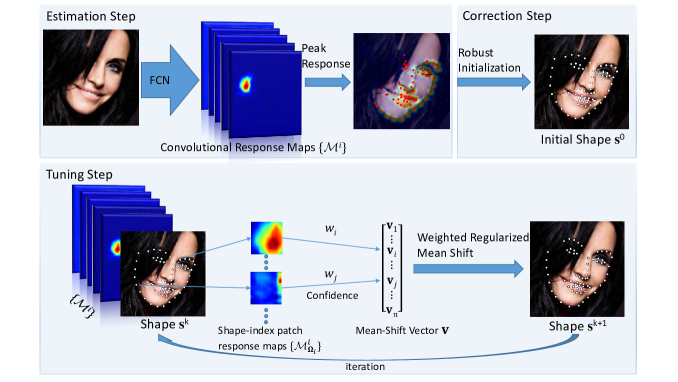
Figure 1: Overview of the proposed ECT (Estimation-Correction-Tuning) approach for facial landmark detection. The framework mainly consists of three steps: 1) The Estimation Step obtains a coarse landmark shape according to the peak response points in the response maps regressed by a fully convolutional network; 2) The Correction Step fits the coarse estimation with the PDM to get a more reasonable initial shape for subsequent procedures; 3) The Tuning Step fine-tunes the landmark shape iteratively based on the proposed weighted regularized mean shift.

II Related work

Facial landmark detection algorithms could be roughly classified into three categories, part-based methods [26, 21], holistic methods [8, 9], and regression-based methods [1, 2, 3, 4, 13, 19]. The part-based methods assemble the outputs from part models and refine the results jointly under certain regulations. The holistic methods manage to optimize a holistic appearance model that best fits the given test face. For regression-based methods, the regressors are typically built to regress the landmark shape directly or predict response maps for each landmark.

II-A Part-based Methods

Our method has an inherent relationship with a sort of part-based methods [7, 10, 11], which typically build a local model for each landmark to suggest the update direction and use a shape model to regulate the result globally. This idea originates from the famous ASM [7] and is extended in CLM [10] to build the more discriminative patch experts. ASM and CLM establish a general framework for facial landmark detection. Different patch experts and more efficient optimization methods have been proposed in recent years [11, 27, 28]. Saragih et al. [11] interpret the CLM in a probabilistic perspective and propose the well-known RLMS via a nonparametric approximation of the response maps. Asthana et al. [28] compress the response maps using dimensionality reduction and regress the shape parameters from the low-dimensional representation of response maps. Baltrusaitis et al. [29] enhance the patch experts using Local Neural Field (LNF) and propose a non-uniform version of RLMS by considering the reliability of patch experts. Recently, they [30] also introduce Convolutional Experts Network (CEN) to replace LNF and achieve higher performances. The weighted term in their non-uniform RLMS is pre-determined and fixed during testing, which is different from our formulation. One limitation of the above mentioned part-based methods is that the utilization of the appearance information is limited in the vicinity of each part. To alleviate this, Alabort-i-Medina et al. [31] propose a unified formulation to merge the holistic and part-based methods. Alternately, we extend the patch experts to make full use of holistic information and utilize the confidence of each expert explicitly to handle the occlusions.

II-B Regression-based Methods

Tackling facial landmark detection as a regression problem is another trend in recent years [1, 3, 12, 4]. Typical approaches [1, 2] use cascaded regressors to predict the coordinates of landmarks directly from shape-indexed features. More recent methods [4, 19, 32] develop strategies such as coarse-to-fine prediction and global-to-local regression to capture information at different scales. On the other hand, Tompson et al. [33] argue that mapping directly from image features to coordinates of joints is highly non-linear and difficult in the context of human pose estimation. Instead of regressing the coordinates, they propose to regress heat-maps, which indicates the per-pixel likelihood of alignment for each body joint. Since then, predicting dense heat-maps via FCN-based networks is exploited for both human pose estimation [22, 34] and facial landmark detection [35, 13, 36, 18]. In [22], Pfister et al. propose to fuse the shallower and deeper layers of the convolutional network to learn spatial dependencies between body parts. In [34], Newell et al. introduce Stacked Hourglass Network for human pose estimation by incorporating multi-resolution features to learn the spacial relationships between joints. For facial landmark detection, Huang et al. [35] introduce a unified FCN framework named DenseBox for simultaneous landmark localization and face detection. Bulat et al. [13] propose a two-step detection-followed-by-regression network to predict the detection scoremap for each landmark. Xiao et al. [16] propose to extract shape-indexed deep features from FCN and refine the landmark locations recurrently via LSTM. In the recent works of [36, 18], Stacked Hourglass Network is also shown to be effective for facial landmark detection. Additionally, landmark heatmaps are used as indicators to help extract discriminative features from images. In [37], Kowalski et al. revise Cascade Shape Regression based methods by stacking the landmark heatmaps with the raw image as input for each stage. Kumar et al. [38] also adopt a similar strategy in an iterative multi-task learning framework to predict the head pose, visibility and position of each landmark simultaneously. The methods mentioned above either build the pre-defined structure model into the network or implicitly exploit the structural constraint by resorting to the elaborate network architectures. In contrast, we propose a framework based on convolutional response maps and explicitly utilize the structure model to regulate the landmark locations with respect to the confidence of the response maps, which is shown to be effective in our experiments.

III Approach

The framework of the proposed ECT approach is shown in Fig. 1. Given an input face image, the landmark detection result is obtained after all three steps of ECT, namely estimation, correction and tuning step. The Estimation Step aims to compute a global localization of the initial landmarks based on the peak response points in the response maps, which are learned from a fully convolutional network (FCN). After that, a more reasonable and accurate initial shape for subsequent procedures is computed by correcting the outlier landmarks using a pre-trained point distribution model (PDM). Finally, the landmark locations are fine-tuned based on the proposed weighted regularized mean shift.

This section firstly introduces the problem formulation for the proposed approach. Then the principal parts of the ECT approach, namely convolutional response map, robust initialization and weighted regularized mean shift, are presented later in detail.

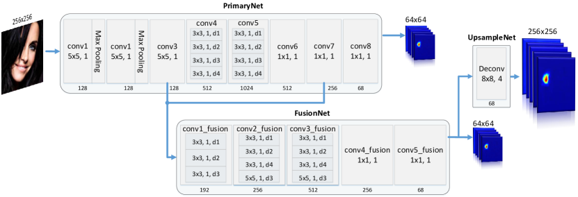
(a)

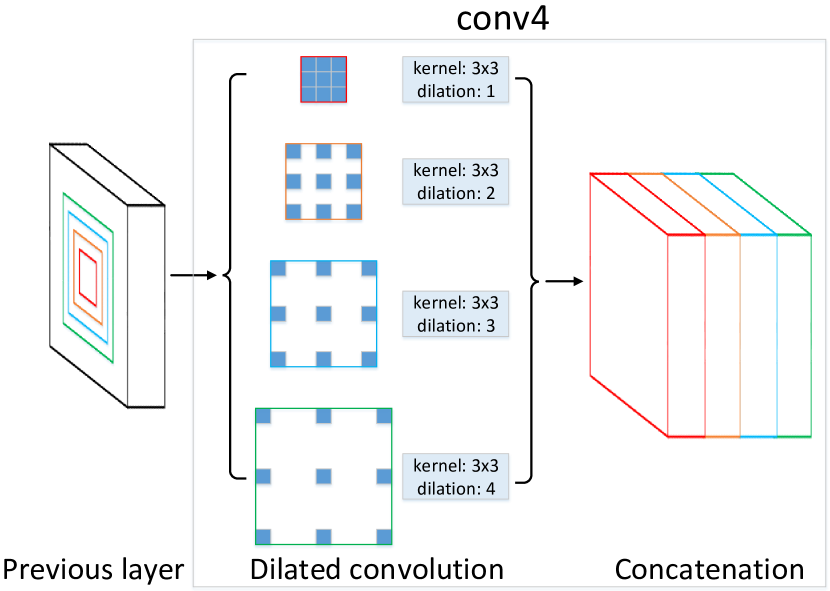
(b)

Figure 2: Architecture of the proposed fully convolutional network (FCN). (a) Overview of our FCN. The filter parameter of each layer is denoted in the form of (kernel size, stride [, d*]) where d* means that there is a dilated convolution with the dilation factor of *. The number below the layer block shows the size of the output channel. ReLU nonlinearity is employed after each convolutional layer except conv8 and conv5_fusion. (b) The Inception module with different dilated convolution filters. Note that dilated convolution with same number of filter parameters could have receptive fields with different sizes.

III-A Problem Formulation

Point distribution model (PDM) [7] is widely used in classic part-based methods. It models the shape with global rigid transformations (scaling, in-plane rotation, and translation) as well as non-rigid variations (head poses and expressions). A 2D shape $\mathbf{s}=[{{\mathbf{x}}_{1}^{\mathsf{T}}},\ldots,{{\mathbf{x}}_{n}^{\mathsf{T}}}]^{\mathsf{T}}\in{{\mathbb{R}}^{2n\times 1}}$ could be considered as the concatenation of $n$ landmarks, with coordinates of the $i$-th landmark written as ${\mathbf{x}}_{i}=[{x}_{i},{y}_{i}]^{\mathsf{T}}$. Further decomposition of ${\mathbf{x}}_{i}$ could be expressed in the following equation:

$$\mathbf{x}_{i}=s\mathbf{R}(\overline{{\mathbf{x}}}_{i}+{\mathbf{\Phi}_{i}\mathbf{q}})+\mathbf{t}$$ (1)

where $\mathbf{p}=\{s,\mathbf{R},\mathbf{t},\mathbf{q}\}$ denotes the parameters of PDM. Concretely, $\mathbf{p}$ consists of a set of global rigid transform parameters (global scaling $s$, rotation $\mathbf{R}$, translation $\mathbf{t}$) and non-rigid parameters $\mathbf{q}$. $\overline{\mathbf{x}}_{i}$ and $\mathbf{\Phi}_{i}$ denote the pertaining sub-matrix of the $i$-th landmark in the mean shape $\overline{\mathbf{s}}$ and the shape components $\mathbf{\Phi}$, respectively. $\mathbf{\Phi}$ is the collection of eigenvectors corresponding to the $m$ largest eigenvalues by applying PCA to a set of training shapes. Given enough training samples, $\mathbf{\Phi}$ is capable of encoding rich expressions. Assuming that the rigid transformation mentioned earlier has a non-informative prior and that the non-rigid shape parameter $\mathbf{q}$ exhibits Gaussian distributions, the PDM parameter $\mathbf{p}$ has the following prior:

$$p(\mathbf{p})\varpropto\mathcal{N}(\mathbf{q};\mathbf{0},\mathbf{\Lambda});\leavevmode\nobreak\ \leavevmode\nobreak\ \mathbf{\Lambda}=\text{diag }\{[{{\lambda}_{1}},\ldots,{{\lambda}_{m}}]\}$$ (2)

where ${\lambda}_{i}$ denotes the eigenvalue of the $i$-th eigenvector in ${\mathbf{\Phi}}$. With this prior knowledge, the parameter $\mathbf{p}$ could be inferred in a Bayesian manner. Assuming the detection results are conditionally independent for each landmark, the posterior distribution of $\mathbf{p}$ could then be written as:

$$p(\mathbf{p}|\{{{l}_{i}}=1,{\mathcal{D}_{i}}\}_{i=1}^{n},\mathcal{I})\propto p(\mathbf{p})\prod\limits_{i=1}^{n}{p({{l}_{i}}=1|{{\mathbf{x}}_{i}},{\mathcal{D}_{i}},\mathcal{I})}$$ (3)

where ${{l}_{i}}\in\{1,-1\}$ indicates whether the $i$-th landmark is aligned or misaligned on coordinate ${\mathbf{x}}_{i}$ for image $\mathcal{I}$, and ${\mathcal{D}}_{i}$ is the given detection expert for the $i$-th landmark.

Assuming that there is a set of candidate coordinates ${{\mathbf{\Psi}}_{i}}$ for the $i$-th landmark, the conditional likelihood $p({{l}_{i}}=1|{{\mathbf{x}}_{i}},{\mathcal{D}}_{i},\mathcal{I})$ could be approximated with a nonparametric representation [11] using Kernel Density Estimator (KDE). Mathematically, the conditional likelihood has the following form:

$$p({{l}_{i}}=1|{{\mathbf{x}}_{i}},{\mathcal{D}}_{i},\mathcal{I})=\sum\limits_{{{\mathbf{y}}_{i}}\in{{\mathbf{\Psi}}_{i}}}{{{\pi}_{{{\mathbf{y}}_{i}}}}\mathcal{N}({{\mathbf{x}}_{i}};{{\mathbf{y}}_{i}},{\rho}_{i}\mathbf{I})}$$ (4)

where ${{\pi}_{{{\mathbf{y}}_{i}}}}=p({{l}_{i}}=1|{{\mathbf{y}}_{i}},{\mathcal{D}}_{i},\mathcal{I})$ is corresponding to the response map (normalized) to be introduced in the next subsection. ${\rho}_{i}=\frac{{\rho}^{2}}{w_{i}}$ is used to smooth the response map, where $\rho$ is a free parameter and $w_{i}$ adjusts the smoothness according to the confidence of the detection expert ${\mathcal{D}}_{i}$ for image $\mathcal{I}$.

Combining Eqs. (3) and (4) gives us the following expression:

$$p(\mathbf{p}|\{{{l}_{i}}=1,{{\mathcal{D}}_{i}}\}_{i=1}^{n},\mathcal{I})\propto p(\mathbf{p})\prod\limits_{i=1}^{n}{\sum\limits_{{{\mathbf{y}}_{i}}\in{{\mathbf{\Psi}}_{i}}}{{{\pi}_{{{\mathbf{y}}_{i}}}}\mathcal{N}({{\mathbf{x}}_{i}};{{\mathbf{y}}_{i}},{\rho}_{i}\mathbf{I})}}$$ (5)

Eq. (5) could be solved iteratively using the EM algorithm and the mean-shift algorithm [11]. In the E-step, the posterior over $\mathbf{y}_{i}$ could be evaluated as follows when treating the candidates $\{\mathbf{y}_{i}\}_{i=1}^{n}$ as hidden variables:

$${{w}_{{{\mathbf{y}}_{i}}}}=p({{\mathbf{y}}_{i}}|{{l}_{i}}=1,{{\mathbf{x}}_{i}},{{\mathcal{D}}_{i}},\mathcal{I})=\frac{{{\pi}_{{{\mathbf{y}}_{i}}}}\mathcal{N}\left({{\mathbf{x}}_{i}};{{\mathbf{y}}_{i}},{\rho}_{i}\mathbf{I}\right)}{\sum\nolimits_{{{\mathbf{z}}_{i}}\in{{\mathbf{\Psi}}_{i}}}{{{\pi}_{{{\mathbf{z}}_{i}}}}\mathcal{N}\left({{\mathbf{x}}_{i}};{{\mathbf{z}}_{i}},{\rho}_{i}\mathbf{I}\right)}}$$ (6)

Then, the M-step works on minimizing the Q function:

$$\begin{split}Q(\mathbf{p})&={{E}_{q(\mathbf{y})}}[-\ln\{p(\mathbf{p})\prod\limits_{i=1}^{n}{p({{l}_{i}}=1,{{\mathbf{y}}_{i}}|{{\mathbf{x}}_{i}},{\mathcal{D}}_{i},\mathcal{I})}\}]\\ &\propto\left\|\mathbf{q}\right\|_{{{\mathbf{\Lambda}}^{-1}}}^{2}+\sum\limits_{i=1}^{n}{{{w}_{i}}\sum\limits_{{{\mathbf{y}}_{i}}\in{{\mathbf{\Psi}}_{i}}}{\frac{{{w}_{{{\mathbf{y}}_{i}}}}}{{\rho}^{2}}{{\left\|{{\mathbf{x}}_{i}}-{{\mathbf{y}}_{i}}\right\|}^{2}}}}\end{split}$$ (7)

where $q(\mathbf{y})=\prod\nolimits_{i=1}^{n}{p({{\mathbf{y}}_{i}}|{{l}_{i}}=1,{{\mathbf{x}}_{i}},{{\mathcal{D}}_{i}},\mathcal{I})}$. The iterative solution $\Delta\mathbf{p}$ for each update could thus be written as:

$$\Delta\mathbf{p}=-{{({\rho}^{2}{{\widetilde{\mathbf{\Lambda}}}^{-1}}+{{\mathbf{J}}^{\mathsf{T}}}\mathbf{WJ})}^{-1}}({\rho}^{2}{{\widetilde{\mathbf{\Lambda}}}^{-1}}\mathbf{p}-{{\mathbf{J}}^{\mathsf{T}}}\mathbf{Wv})$$ (8)

In the above equation, $\widetilde{\mathbf{\Lambda}}=\text{diag}\{[\mathbf{0},{{\lambda}_{1}},\ldots,{{\lambda}_{m}}]\}$, $\mathbf{J}=[\mathbf{J}_{1},\ldots,\mathbf{J}_{n}]$, where $\mathbf{J}_{i}$ is the Jacobian of PDM in Eq. (1), $\mathbf{W}=\text{diag}\{[{{w}_{{{x}_{1}}}},{{w}_{{{y}_{1}}}},\ldots,{{w}_{{{x}_{n}}}},{{w}_{{{y}_{n}}}}]\}$ with ${w}_{{{x}_{i}}}={w}_{{{y}_{i}}}={w}_{i}$, $\mathbf{v}=[{\mathbf{v}}_{1}^{\mathsf{T}},\ldots,{\mathbf{v}}_{n}^{\mathsf{T}}]^{\mathsf{T}}$ is the mean shift vectors of all landmarks:

$${{\mathbf{v}}_{i}}=\left(\sum\limits_{{{\mathbf{y}}_{i}}\in{{\mathbf{\Psi}}_{i}}}{\frac{{{\pi}_{{{\mathbf{y}}_{i}}}}\mathcal{N}\left(\mathbf{x}_{{{\mathbf{y}}_{i}}}^{c};{{\mathbf{y}}_{i}},{\rho}_{i}\mathbf{I}\right)}{\sum\nolimits_{{{\mathbf{z}}_{i}}\in{{\mathbf{\Psi}}_{i}}}{{{\pi}_{{{\mathbf{z}}_{i}}}}\mathcal{N}\left(\mathbf{x}_{i}^{c};{{\mathbf{z}}_{i}},{\rho}_{i}\mathbf{I}\right)}}}{{\mathbf{y}}_{i}}\right)-\mathbf{x}_{i}^{c}$$ (9)

where $\mathbf{x}_{i}^{c}$ is the currently estimated position of the $i$-th landmark.

Eqs. (8) and (9) demonstrate that our algorithm alternates between computing the move step from response maps and regularizing it with the shape model’s constraint. The main difference between our formulation and RLMS [11] is that a weight value is assigned to each landmark mean-shift vector before it is projected onto the subspace spanned by the PDM’s Jacobian, which contributes a key factor to the success in robust facial landmark detection. Note that the weights are updated in each tuning step, which is different from the non-uniform RLMS [29]. Specifically, the mean-shift vector calculated from response maps is selectively projected onto the PCA space according to the latest weight matrix $\mathbf{W}$, so that the tuning step could effectively reach the balance between the efforts from detection experts and the global prior information from PDM.

III-B Convolutional Response Map

Regression-based methods [1, 12, 2] train regressors to predict the landmark location $\mathbf{x}_{i}$ directly. Following the previous work [22, 13], the regressor FCN in our method, namely the part detection expert, is used to regress the ideal response map for each landmark in a data-driven manner. The ideal response map of the $i$-th landmark for image $\mathcal{I}$ is a single-channel image $\mathcal{M}^{i}$ with the same resolution as $\mathcal{I}$, and its pixel value at position $\mathbf{z}$ is defined as $\mathcal{M}_{\mathbf{z}}^{i}=\mathcal{N}(\mathbf{z};{{\mathbf{x}}_{i}^{*}},{{\sigma}^{2}}\mathbf{I})$, where $\mathbf{x}_{i}^{*}$ is the ground truth location of the $i$-th landmark, and $\sigma$ serves to control the scope of the response.

Fig. 2(a) shows an overview of the proposed FCN architecture. Our FCN network consists of three connected subnetworks, namely the PrimaryNet, FusionNet and UpsampleNet. Given an input image with the size of $256\times 256$, the first two subnetworks regress the smaller response maps with the size of $64\times 64$. The last UpsampleNet is simply a deconvolutional layer which bilinearly upsamples the feature maps back to the size of the input image.

Given the training dataset $N=\{(\mathcal{I},\mathbf{s}^{*})\}$, where $\mathbf{s}^{*}$ is the ground truth shape embedded in image $\mathcal{I}$, the objective of the regressor becomes estimating the network weights $\lambda$ that minimize the following L2 loss function:

$$\mathcal{L}(\lambda)=\sum\limits_{(\mathcal{I},{{\mathbf{s}}^{*}})\in N}{\sum\limits_{i}{{{\left\|{{\mathcal{M}}^{i}}-{{\phi}^{i}}(\mathcal{I},\lambda)\right\|}^{2}}}}$$ (10)

where ${\phi}^{i}(\mathcal{I},\lambda)$ is the output of the $i$-th channel of the regression network fed with the image $\mathcal{I}$. The loss functions for the PrimaryNet and FusionNet have the same loss function as expressed in (10) with downsampled spatial resolutions.

The design of the PrimaryNet and FusionNet is originated from the pose estimation networks [22] and adapted to the case of facial landmark detection. As mentioned in [22], the PrimaryNet can not learn the spatial dependencies of landmarks very well. To address this problem, conv3 and conv7 are firstly concatenated and then fed to the FusionNet. The main difference between the architectures of our subnetworks and the pose estimation networks [22] is that we adopt the Inception module [39] with different dilated convolution filters [40] for layer conv4, conv5, conv1_fusion, conv2_fusion and conv3_fusion. All these dilated convolution sub-layers are concatenated together so that the next layer could extract features from different scales simultaneously (see illustration in Fig. 2(b)). Such an improvement could achieve a comparable regression result with the size of the model reduced by half. The benefit of using dilated convolution is significant, as it supports exponential expansion of the receptive field with the number of parameters growing linearly. These dilated convolution filters are well-suited for landmark detection task which requires pixel level texture information in multiple scales.

in 2,3,4,5

(a)

Figure 3: Robust initialization. (a)-(c) show the result of locating the landmarks according to the peak responce points, projecting the landmarks onto the PDM space, and correcting them using non-uniform regularization to obtain the initial shape, respectively. The response maps of all landmarks are superimposed over each other for better visualization. (d) shows the provided ground truth (red) and the initial shape (white) together with the face image.

in 2,3,1,4,5,6,7 in 2,3,1,4,5,6,7

Figure 4: Visualization of the detection confidence of different facial landmarks. The upper row shows the superimposed response maps of all landmarks. The lower row shows the landmark position and the reliability calculated at the final stage. The radius of a landmark is inversely proportional to its reliability.

III-C Robust Initialization

At inferrence time, the image $\mathcal{I}$ is fed into a pre-trained FCN to obtain the response maps $\mathcal{M}=\{{\mathcal{M}}^{i}\}$. The facial landmarks are firstly located at the peak response positions in the response maps and then fitted into the PDM to obtain a more reasonable and accurate landmark shape as initialization. Generally, the coarsely estimated shape $\mathbf{s}$ could be regularized with the PDM directly by minimizing the reconstruction error. However, such a regularization treats each landmark equally without considering their reliabilities. For a more robust initialization, a non-uniform regularization is proposed by minimizing the following reconstruction error:

$$\underset{s,\mathbf{R},\mathbf{t},\mathbf{q}}{\mathop{\arg\min}}\,\left\|\mathbf{s}-s\widetilde{\mathbf{R}}(\overline{\mathbf{s}}+\mathbf{\Phi q})-\widetilde{\mathbf{t}}\right\|_{\mathbf{W}}^{2}$$ (11)

where $\widetilde{\mathbf{R}}$ and $\widetilde{\mathbf{t}}$ are repeated copies of the rotation matrix $\mathbf{R}$ and translation vector $\mathbf{t}$ respectively, and $\mathbf{W}$ is a diagonal weight matrix where the diagonal elements are the weights of corresponding facial landmarks. Note that the weight matrix is estimated in the same way as the $\mathbf{W}$ in Eq. 8 and will be described in detail in the next subsection. Adding the regularization term gives us the following objective function:

$$\underset{s,\mathbf{R},\mathbf{t},\mathbf{q}}{\mathop{\arg\min}}\,\left\|\mathbf{s}-s\widetilde{\mathbf{R}}(\overline{\mathbf{s}}+\mathbf{\Phi q})-\widetilde{\mathbf{t}}\right\|_{\mathbf{W}}^{2}+\gamma\left\|\mathbf{q}\right\|_{{{\mathbf{\Lambda}}^{-1}}}^{2}$$ (12)

where $\gamma$ is used to balance the two norms.

The optimal parameters of Eq. (12) could be obtained by iteratively solving the global similarity transform parameters $\{s,\mathbf{R},\mathbf{t}\}$ and non-rigid parameters $\mathbf{q}$. Using the orthonormalization of the global similarity transform [41], the shape model (Eq. (1)) could be compactly written as:

$$\mathbf{s}=\overline{\mathbf{s}}+\mathbf{S}\mathbf{p}$$ (13)

where $\mathbf{S}=[\mathbf{s}_{1}^{*},\ldots,\mathbf{s}_{4}^{*},\mathbf{\Phi}]\in{{\mathbb{R}}^{2n\times(4+m)}}$ is the concatenation of the similarity bases $\mathbf{s}_{i}^{*}$ with the original shape components $\mathbf{\Phi}$, and $\mathbf{p}=[p_{1}^{*},\ldots,p_{4}^{*},\mathbf{q}^{\mathsf{T}}]^{\mathsf{T}}\in{{\mathbb{R}}^{(4+m)\times 1}}$ is re-defined as the concatenation of the similarity parameters $p_{i}^{*}$ with the non-rigid shape parameter $\mathbf{q}$. Following the above decomposition, the optimal parameters of the initial shape ${\mathbf{s}}^{0}$ have the closed form:

$${{\mathbf{p}}^{0}}={{(\gamma{{\widetilde{\mathbf{\Lambda}}}^{-1}}+{{\mathbf{S}}^{\mathsf{T}}}\mathbf{WS})}^{-1}}{{\mathbf{S}}^{\mathsf{T}}}\mathbf{Ws}$$ (14)

Note that Eq. (14) is equivalent to Eq. (8) when substituting $\mathbf{x}_{i}^{c}$ and $\mathbf{p}$ with $\mathbf{0}$ and regarding the move step $\mathbf{v}$ as $\mathbf{s}$.

Fig. 3 demonstrates the effect of the robust initialization. It could be seen that the proposed non-uniform regularization is able to correct the location error of outliers so that they could more accurately locate within the vicinity of the ground truth. Such a correction step could provide a more reasonable initial shape for subsequent procedures and reduce the chance of failing during testing.

III-D Weighted Regularized Mean Shift

After computing the initial shape $\mathbf{s}^{0}$ from the correction step, the estimated shape is then fine-tuned iteratively using the weighted regularized mean shift.

In the $k$-th stage, the currently estimated shape $\mathbf{s}^{k}$ is obtained and the shape-index patch response maps are extracted from $\mathcal{M}$ for each landmark. The shape-index patch response map $\{\pi_{\mathbf{y}_{i}}\}$ for the $i$-th landmark is a $r\times r$ square subarea centered at $\mathbf{x}_{i}^{k}$ in the response map ${\mathcal{M}}^{i}$. For those areas which are partially out of the range of ${\mathcal{M}}^{i}$ (e.g. $\mathbf{x}_{i}^{k}$ is close to the boundary of ${\mathcal{M}}^{i}$ when $r$ is large enough), the missing parts are padded with zeros. The collection of all coordinates in the square subarea for the $i$-th landmark is denoted as $\mathbf{\Omega}_{i}$. Inspired by the work in [3], the patch size $r$ is progressively shrinked from early stage to later stage.

For each shape-index patch response map, its confidence $w_{i}$ is estimated empirically as follows:

$${{w}_{i}}=sigmoid(a\frac{\sum\nolimits_{{{\mathbf{y}}_{i}}\in{{\mathbf{\Omega}}_{i}}}{{{\pi}_{{{\mathbf{y}}_{i}}}}}}{{{\operatorname{var}}_{{{\mathbf{y}}_{i}}\in{{\mathbf{\Omega}}_{i}}}}({\mathbf{y}_{i}},{{\pi}_{{{\mathbf{y}}_{i}}}})}+b)$$ (15)

where ${\operatorname{var}}_{{{\mathbf{y}}_{i}}\in{{\mathbf{\Omega}}_{i}}}({\mathbf{y}_{i}},{{\pi}_{{{\mathbf{y}}_{i}}}})$ denotes the variance of the patch response map, $a$ and $b$ are two empirical parameters which could be optimized via cross-validation. Eq. (15) suggests that the confidence of a local expert is proportional to the sum of its response values and inversely proportional to the degree of dispersion of its spatial distribution. Sigmoid function is used to normalize the confidence values within the range of $(0,1)$. Fig. 4 visualizes the detection confidence of different facial landmarks on several examples. It could be observed that those blurred or invisible parts are able to be differentiated from others easily.

After calculating the weights, the mean shift vectors $\mathbf{v}_{i}$ are computed for all landmarks using Eq. (9), where the candidate coordinates ${{\mathbf{\Psi}}_{i}}$ are set equal to ${\mathbf{\Omega}_{i}}$, and the response map $\{\pi_{\mathbf{y}_{i}}\}$ is normalized so that $\sum\nolimits_{{{\mathbf{y}}_{i}}\in{{\mathbf{\Psi}}_{i}}}{{{\pi}_{{{\mathbf{y}}_{i}}}}}=1$. The confidence $w_{i}$ is assigned to each mean shift vector $\mathbf{v}_{i}$, and the update $\Delta\mathbf{p}$ for PDM parameters could be computed with the projection in Eq. (8). Finally the latest estimated shape $\mathbf{s}^{k+1}$ is obtained for the next iteration by applying the incremental version of Eq. (1).

The fine-tuning process could converge to stable outcomes after a number of iterations. A desirable result could typically be achieved within 5 iterations in our experiments. The complete process of our algorithm is summarized in Algorithm 1.

Algorithm 1 ECT (Estimation-Correction-Tuning) for facial landmark detection.

The pre-trained FCN and PDM, the input face image $\mathcal{I}$

 

The facial shape $\mathbf{s}$
$\triangleright$ Estimation step

1:Feed $\mathcal{I}$ into FCN and get the response maps $\{\mathcal{M}^{i}\}$

2:Obtain the coarse shape by locating the landmarks at the peak response positions in $\{\mathcal{M}^{i}\}$

$\triangleright$ Correction step

3:Regularize the coarse shape with PDM and get the initial shape $\mathbf{s}^{0}$ using Eq. (14)

$\triangleright$ Tuning step

4:for $k=0\leavevmode\nobreak\ to\leavevmode\nobreak\ K$ do

5:     for the $i$-th landmark do

6:         Calculate shape-index patch coordinates $\mathbf{\Omega}_{i}$

7:         Extract patch response map $\{{\pi}_{\mathbf{y}_{i}}=\mathcal{M}_{\mathbf{y}_{i}}^{i}\}$ where ${{{\mathbf{y}}_{i}}\in{{\mathbf{\Omega}}_{i}}}$

8:         Calculate $w_{i}$ and $\mathbf{v}_{i}$ from $\{{\pi}_{\mathbf{y}_{i}}\}$, using Eqs. (15) and (9) respectively

9:     end for

10:     Calculate $\Delta\mathbf{p}$ using Eq. (8)

11:     Update PDM parameters $\mathbf{p}^{k+1}=\mathbf{p}^{k}+\Delta\mathbf{p}$

12:     Update shape $\mathbf{s}^{k+1}$ using Eq. (1)

13:end for

IV Experiments

Datasets. The evaluation experiments are conducted on four benchmark datasets, 300W [23], AFLW [24], AFW [21] and COFW [25], to demonstrate the effectiveness of the proposed method on challenging face images in natrual scenes.

• 300W [23]: The 300W dataset contains near-frontal face images in the wild and provides 68 annotated points for each face. To keep consistent with previous work, the datasets are partitioned and renamed as follows. The 300W training set contains 3,148 training images from AFW [21], LFPW [42] and HELEN [43]. The common subset of 300W contains 554 test images from LFPW and HELEN. The challenging subset of 300W contains 135 test images from IBUG [23]. The fullset of 300W is the union of the common and challenging subset. The 300W test set contains 600 test images which are provided officially by the 300W competition [23] and said to have a similar distribution to the IBUG dataset.

• AFLW [24]: The original AFLW dataset contains about $25k$ in-the-wild faces with a wide range of head pose and provides up to 21 annotated points visible on each face. A subset of AFLW with a balanced distribution of head pose is selected in [44] and is denoted as AFLW-PIFA. Additional 13 landmarks are labeled later in [45] so that 34 landmarks and their visible/invisible states are provided in AFLW-PIFA. For the evaluation on AFLW, 3,901 training images of AFLW-PIFA are used for training and the remaining 1,299 images are used for testing.

• AFW [21]: The AFW dataset is a popular benchmark for facial landmark detection, containing 468 faces of all pose ranges in 205 images. A detection bounding box as well as up to 6 visible landmarks are provided for each face. The AFW dataset is only used for testing in our experiments due to the small number of samples.

• COFW [25]: The COFW dataset contains in-the-wild face images with heavy occlusions, including 1345 face images for training and 507 face images for testing. For each face, 29 landmarks and the corresponding occlusion states are annotated in the COFW dataset.

Evaluation metric. For fair comparison, the evaluation metrics are chosen as the common protocols in the literature [1, 27, 23, 46, 45]. The primary metric is the Normalized Mean Error (NME), which could be calculated as $\frac{1}{n}\sum\nolimits_{i=1}^{n}{\frac{{{\left\|{{\mathbf{x}}_{i}}-\mathbf{x}_{i}^{*}\right\|}_{2}}}{d}}$, where $d$ denotes the normalized distance and $n$ is the number of facial landmarks involved in the evaluation. Other evaluation metrics such as the Mean Average Pixel Error (MAPE), the Cumulative Error Distribution (CED) curve, the Area-Under-the-Curve (AUC) calculated from the CED curve and the failure rate are also reported in experiments for thorough analysis.

Implementation details. The FCN in our experiments is implemented using the Caffe framework [47]. The FCN takes the input of a $256\times 256$ face image and outputs a set of response maps with the same resolution. To avoid overfitting, we randomly flip the input image horizontally and crop a $248\times 248$ arbitrary sub-image from it. Then, we rotate it with a random angle from $-30^{\circ}$ to $30^{\circ}$ before rescaling it back to $256\times 256$. The variance $\sigma$ of the 2D Guassians in ideal response maps is set to $6$. For those facial landmarks marked as invisible in the AFLW and COFW datasets, the ideal responses are re-defined as zeros instead of the 2D Gaussian responses. During training of the FCN, the learning rate is fixed to $10^{-8}$ and the momentum is set to 0.95. The parameter $a$ and $b$ in Eq. (15) is set to 0.25 and 25 respectively in our experiments. The weighted regularized mean shift algorithm is implemented based on the Menpo project [48]. Code has been made publicly available.

Table I: Comparison of AUC (%) and failure rate (%) on the test set of the 300W competition. The results of other methods are obtained from [14, 37].

	51 points		68 points
Method	AUC	Failure rate	AUC	Failure rate
ERT [49]	40.60	13.50	32.35	17.00
PO-CR [50]	47.65	11.70	-	-
SDM [2]	38.47	19.70	-	-
CLNF [29]	37.65	17.17	19.55	38.83
CFSS [5]	50.79	7.80	39.81	12.30
MDM [14]	56.34	4.20	45.32	6.80
DAN [37]	-	-	47.00	2.67
ECT	58.26	1.17	45.98	3.17

Table II: Comparison of NME (%) with state-of-the-art methods on the fullset of 300W.

Method	Common Subset	Challenging Subset	Fullset
CDM [27]	10.10	19.54	11.94
TSPM [21]	8.22	18.33	10.20
Smith et al. [51]	-	13.30	-
DRMF [28]	6.65	19.79	9.22
GN-DPM [26]	5.78	-	-
CLNF [29]	-	-	10.95
RCPR [25]	6.18	17.26	8.35
CFAN [4]	5.50	16.78	7.69
ESR [1]	5.28	17.00	7.58
SDM [2]	5.57	15.4	7.50
ERT [49]	-	-	6.40
LBF [3]	4.95	11.98	6.32
CFSS [5]	4.73	9.98	5.76
TCDCN [6]	4.80	8.60	5.54
3DDFA [52]	5.53	9.56	6.31
DDN [53]	-	-	5.65
RAR [16]	4.12	8.35	4.94
JFA [32]	5.32	9.11	6.06
DAN [37]	4.42	7.57	5.03
TR-DRN [19]	4.36	7.56	4.99
DeFA [54]	5.37	9.38	6.10
PIFA-S [55]	5.43	9.88	6.30
RDR [56]	5.03	8.95	5.80
ECT	4.66	7.96	5.31

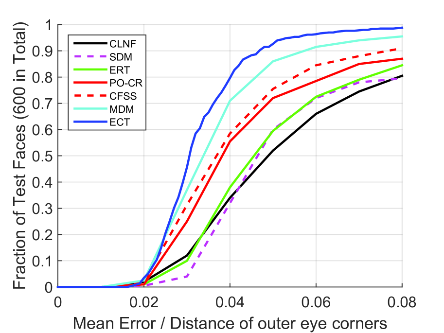
(a) The 300W test set, 51 points

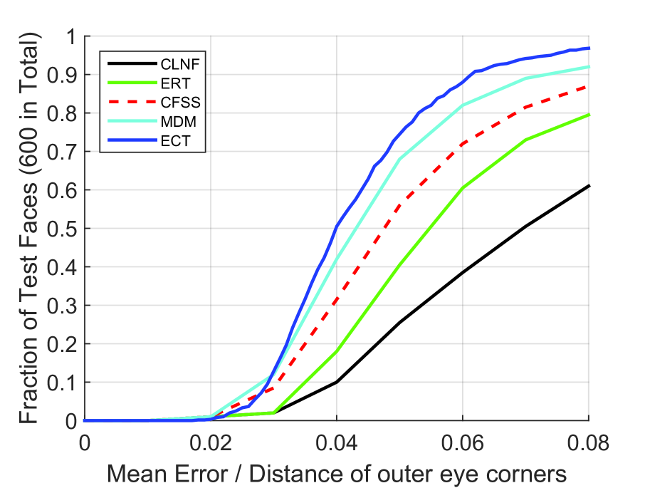
(b) The 300W test set, 68 points

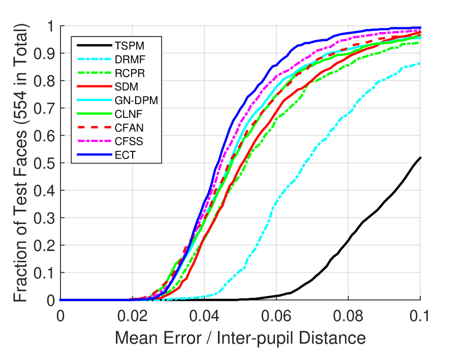
(c) The common subset

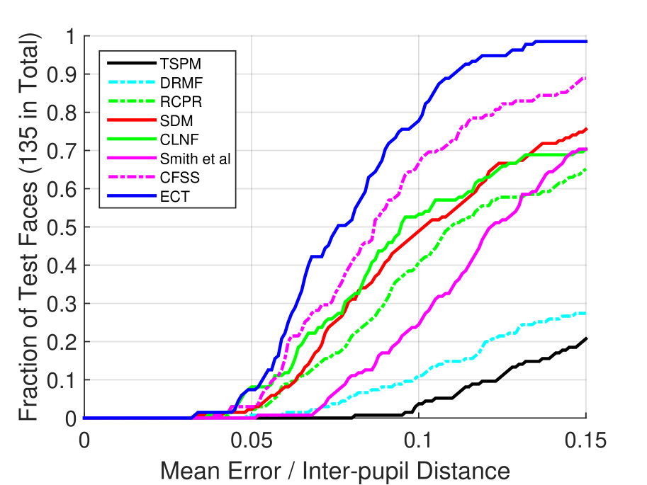
(d) The challenging subset

Figure 5: Comparison of cumulative errors distribution (CED) curves on 300W. (a)(b) show CED curves of existing methods on the 300W test set for 51 points and 68 points. (c)(d) show CED curves of existing methods on the common subset and the challenging subset of 300W.

IV-A Comparison with Existing Methods

We compare our approach with existing methods including CLNF [29], CDM [27], SDM [2], LBF [3], RCPR [25], TCDCN [6], DDN [53], MDM [14], RAR [16], PIFA-S [55], RDR [56], etc. Among these algorithms, CLNF and CDM are two part-based methods built upon the revised part models and parametric shape models. SDM and LBF are two representative cascaded regression methods. RCPR is a regression-based method aimed at handling occlusions. TCDCN is a deep learning based method using multi-task learning. DDN is a cascaded method incorporating structural constraints within the CNN framework. MDM and RAR are two state-of-the-art methods using recurrent neural networks to refine the landmark prediction. PIFA-S and RDR are two pose-invariant methods utilizing the 3D face model.

IV-A1 Evaluation on 300W

The evaluation on 300W consists of two parts. The first part is conducted on the 300W test set provided officially by the 300W competition [23]. The second part of the evaluation is performed on the fullset of 300W which is widely used in the literature.

For the 300W test set, the error is normalized by the distance of outer corners of the eyes to maintain consistency with the 300W competition. The evaluation metrics used are the AUC and failure rate as in [14]. The AUC stands for the area-under-the-curve of CED curves, and the failure rate is calculated with the threshold set to 0.08 for the normalized point-to-point error. The comparison results with different methods for both 51 points and 68 points are reported in Table I. Experimental results show that our method is narrowly beaten by DAN [37] and outperforms other state-of-the-art methods including PO-CR [50], CFSS [5] and MDM [14] especially on failure rate.

For the fullset of 300W, we compare the localization results on the common subset, the challenging subset and the fullset. For fair comparison, the localization error is normalized by the inter-pupil distance, which is consistent with previous works [3, 5]. Since the pupil landmark positions are not available in the 300W dataset, they are instead estimated by averaging the coordinates of the landmarks around the eyes [3, 5]. The comparison with various state-of-the-art methods are reported in Table II. It should be noted that the performance on the fullset of 300W is nearly saturated for the end-to-end methods proposed recently. Our method achieves a comparable result in comparison with the most recent state-of-the-art methods RAR [16], DAN [37] and TR-DRN [19], and shows superior performance to others.

Cumulative error distribution (CED) curves of different methods on 300W are also plotted in Fig. 5. As can be seen, the performance of ECT is superior to other approches particularly on the 300W test set and the challenging subset, which means ECT is robust to various challenging conditions such as exaggerated expressions or occlusions. Fig. 6 shows example results of the proposed method on 300W.

Table III: Comparison of NME (%) with state-of-the-art methods on AFLW. Results of other methods are obtained from literature [46, 45, 13].

	AFLW-PIFA
Method	21 points (vis.)	34 points (vis.)
CDM [27]	8.59	-
RCPR [25]	7.15	6.26
CFSS [5]	6.75	-
ERT [49]	7.03	-
SDM [2]	6.96	-
LBF [3]	7.06	-
PIFA [44]	6.52	8.04
PAWF [45]	-	4.72
CCL [46]	5.81	-
CALE [13]	2.63	2.96
KEPLER [38]	2.98	-
PIFA-S [55]	-	4.45
DeFA [54]	-	3.86
ECT	3.21	3.36

IV-A2 Evaluation on AFLW

We evaluate our method on AFLW-PIFA [44] to demonstrate its effectiveness on face images with challenging appearance and head pose variations. During testing, only the visible landmarks are involved in the evaluation. To be consistent with previous works [44, 46], the normalized distance is the square root of the bounding box size, calculated as $\sqrt{w_{bbox}*h_{bbox}}$. The comparison with existing methods for both 21 and 34 points are shown in Table III. It can be observed that ECT achieves results comparable to the latest state-of-the-art methods CALE [13] and KEPLER [38], and outperforms pose-invariant approaches CDM [27], CCL [46], 3D approaches PIFA [44], PAWF [45] and PIFA-S [55] by a large margin. It should be noted that CALE develops a much deeper neural network with the model size an order of magnitude larger than ours. For comparison on landmark detection error across poses, three subsets are divided according to their absolute yaw angles: [0°, 30°], [30°, 60°], and [60°, 90°] with each subset containing 433 samples. Comparison of landmark detection error of 21 points visible on AFLW across poses is reported in Table IV. Note that the results of RCPR, ESR, and SDM are derived from [52] and these algorithms have been adapted to large poses by retraining them on 300W-LP [52]. As shown in Table IV, the proposed method outperforms other algorithms consistently across poses. Fig. 7 shows example results of the proposed method on the AFLW-PIFA dataset.

Table IV: Comparison of NME (%) on AFLW across poses. Results of other methods are obtained from [52, 57, 58, 56].

Method	[0°, 30°]	[30°, 60°]	[60°, 90°]	mean	std
CDM [27]	8.15	13.02	16.17	12.44	4.04
RCPR [25]	5.43	6.58	11.53	7.85	3.24
ESR [1]	5.66	7.12	11.94	8.24	3.29
SDM [2]	4.75	5.55	9.34	6.55	2.45
3DDFA [52]	4.75	4.83	6.38	5.32	0.92
HyerFace [57]	3.93	4.14	4.71	4.26	0.41
3DSTN [58]	3.55	3.92	5.21	4.23	0.87
RDR [56]	3.63	4.29	5.31	4.41	-
ECT	2.94	2.84	3.85	3.21	0.56

Table V: Comparison of NME (%) and MAPE (pixels) with state-of-the-art methods on AFW. Results of other methods are obtained from [46, 45] and respective papers.

Method	NME (%)	MAPE (pixels)
TSPM [21]	-	11.09
CDM [27]	5.70	9.13
RCPR [25]	3.87	-
CFSS [5]	3.43	-
ERT [49]	3.25	-
SDM [2]	3.88	-
LBF [3]	3.39	-
PIFA [44]	-	8.61
PAWF [45]	-	7.43
CCL [46]	2.45	-
KEPLER [38]	3.01	-
PIFA-S [55]	-	6.27
ECT	2.62	5.90

IV-A3 Evaluation on AFW

We further test our method on AFW using the model trained on AFLW-PIFA. Following the setting of previous works [27, 46, 45], we pick out 6 visible landmarks for evaluation on AFW. We report both the Normalized Mean Error (NME) and the Mean Average Pixel Error (MAPE) for comparison in Table V. For NME, the normalized distance is the square root of the bounding box size provided in the AFW dataset. For MAPE, the average of landmark detection errors is calculated at the original image scale. As shown in Table V, the proposed method achieves at least a comparable, or a superior performance in comparison with other state-of-the-art methods including CCL [46], KEPLER [38] and PIFA-S [55]. Example results of the proposed method on AFW is shown in Fig. 8.

IV-A4 Evaluation on COFW

We conduct experiments on the COFW dataset to quantitatively demonstrate the effectiveness of the proposed method on face images with heavy occlusions. 507 face images from the test set of COFW are used for evaluation. Table VI shows the comparison of the landmark detection error, failure rate and occlusion prediction accuracy on COFW. The mean error is normalized with respect to the inter-pupil distance and the failure rate is calculated with the threshold set to 10% of the normalized mean error. In our method, the occlusion status of the landmarks are simply predicted by thresholding the confidence (i.e. Eq. (15)) of the patch response maps in the final stage. It can be seen that the proposed method achieves a nearly saturated landmark detection performance and a significantly higher occlusion prediction accuracy (recall of 63.4% vs. 49.11% at precision = 80%) compared with the previous methods including Wu et al. [59], RCPR [25], RAR [16] and SimLPD [60]. Example results of our method are depicted in Fig. 9.

Table VI: Comparison of facial landmark detection and occlusion prediction results on COFW. The results of TSPM, CDM, ESR, and SDM are obtained from [6].

Method	NME (%)	Failure Rate (%)	Precision/Recall (%)
Human [25]	5.60	-	-
TSPM [21]	14.4	-	-
CDM [27]	13.67	-	-
ESR [1]	11.2	-	-
SDM [2]	11.14	-	-
RCPR [25]	8.5	20	80/40
OC [61]	7.46	13.24	80.8/37.0
RPP [62]	7.52	16.20	78/40
Wu et al. [59]	5.93	-	80/49.11
TCDCN [6]	8.05	-	-
RAR [16]	6.03	4.14	-
SimLPD [60]	6.40	-	80/44.43
ECT	5.98	4.54	80/63.4

Table VII: Comparison of network complexity (number of parameters), runtime (time spent on GPU and CPU) and speed (faces per second) with other deep learning based methods. Numbers are obtained from respective papers or evaluated based on the released codes.

		Runtime
Method	#Parameter	GPU	CPU	FPS
CFAN [4]	$\sim$18M	0	23ms	43
TCDCN [6]	$\sim$0.1M	0	18ms	56
3DDFA [52]	-	23ms	52ms	13
DDN [53]	-	-	-	770
RAR [16]	-	-	-	4
CALE [13]	$\sim$140M	-	-	3
HyperFace [57]	-	-	-	5
KEPLER [38]	-	-	-	4
TR-DRN [19]	$\sim$99M	-	-	83
DAN [37]	$\sim$22M	-	-	45
3DSTN [58]	-	-	-	52
RDR [56]	-	31ms	142ms	6
PIFA-S [55]	-	-	-	4.3
ECT	$\sim$9.5M	30ms	53ms	12

in 1,2,3,4,5,6,7

Figure 6: Example results of the proposed method on the 300W dataset. The images are from the common subset (the top row), the challenging subset (the middle row), and the 300W testset (the bottom row), respectively.

in 8,9,10,11,12,13,14

in 15,16,17,18,19,20,21

in 1,2,3,4,5,6,7

Figure 7: Example results of the proposed method on the AFLW-PIFA dataset. Note that all landmarks are localized from a 3D perspective.

in 8,9,10,11,12,13,14

in 1,2,3,4,5,6,7

Figure 8: Example results of the proposed method on the AFW dataset.

in 1,2,3,4,5,6,7

Figure 9: Example results of the proposed method on the COFW dataset. Green/red points indicate the visible/invisible landmarks predicted by the algorithm.

in 8,9,10,11,12,13,14

IV-A5 Time Complexity

Our method can run in realtime, with the speed of 12fps tested on an Intel Xeon 2.20GHz CPU and an NVIDIA TITAN X GPU. Comparison of network complexity and runtime with other deep learning based methods is reported in Table VII. It can be seen that our method has a more moderate computation cost while achieving promising performances. The most computationally expensive part of our method is generating the response maps. It takes about 30ms for the FCN to process a 256x256 face image on GPU. Using a shallower FCN could further reduce both the model size and runtime with only a slight drop in performance, as pointed out in the next subsection. In our Python implementation of the weighed regularized mean shift, each iteration takes about 15ms to run on CPU. Parallel processing of each landmark or conducting the weighted regularized mean shift on GPU could greatly reduce the runtime of the post-processing stage. Tricks like using sparser candidate landmark sets or a precomputed grid for table lookup could further accelerate the fitting algorithm, as mentioned in [11].

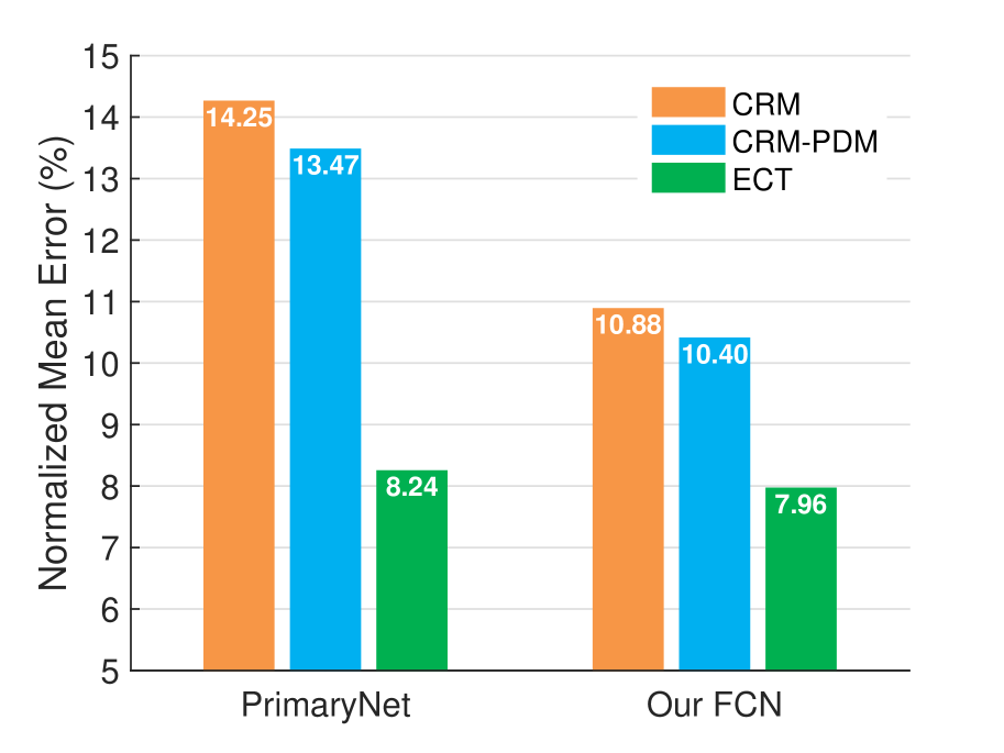
(a)

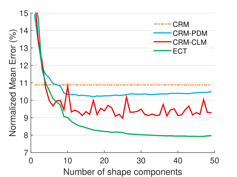
(b)

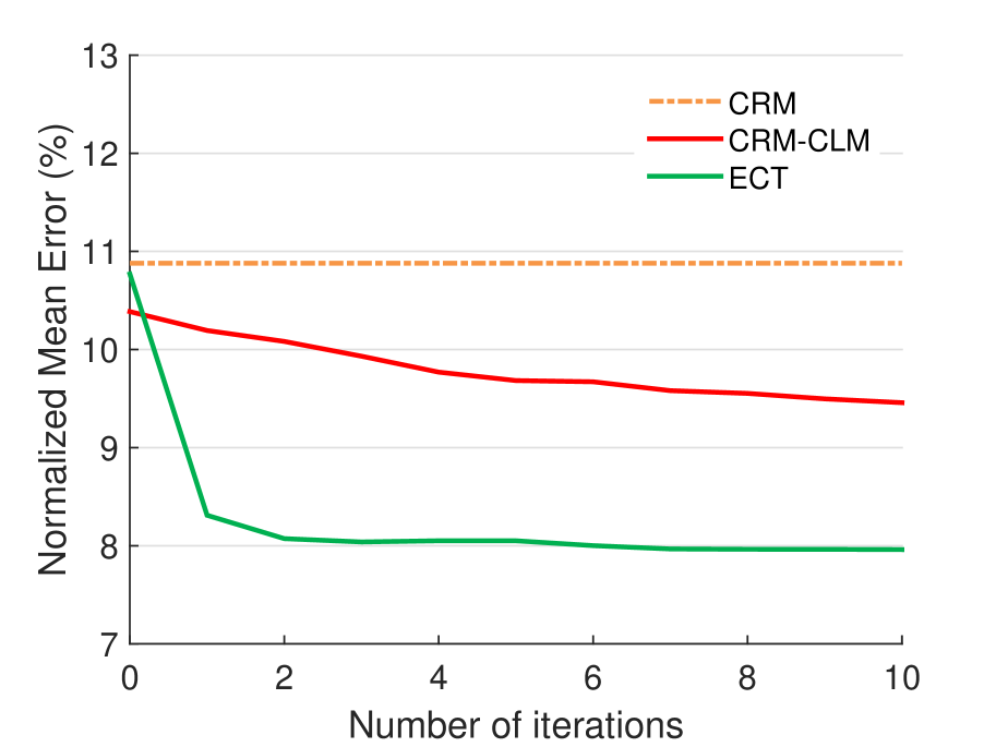
(c)

Figure 10: Component analysis of the proposed method on the challenging subset of 300W. (a) Performance of methods based on the proposed FCN and its subnetwork PrimaryNet. (b) Performance across the number of shape components. (c) Performance across iterations in the tuning step.

Table VIII: Comparison of NME (%) to validate the key components of the proposed method.

Experiment	Common Subset	Challenging Subset	Fullset
CRM(Baseline)	6.61	10.88	7.44
CRM-PDM	6.35	10.40	7.15
CRM-CLM	5.28	9.49	6.10
CRM-CLM-C	5.00	8.32	5.65
ECT	4.66	7.96	5.31

in 1,3,4,5 in img,heatmap,peak,pdm,init,ect
in Input images,Response maps,CRM,CRM-PDM,CRM-Correction,ECT

Figure 11: Qualitative evaluation for ablation study of the proposed method. The images shown in Column 1 are input images. The response maps superimposed on the input images are shown in Column 2. The detection results of CRM and CRM-PDM are shown in Column 3 and 4, respectively. Column 5 shows the results obtained from the correction step of ECT. The results of the proposed ECT method are shown in the last column.

IV-B Ablation Study

It is interesting to investigate the contribution of each module of the proposed ECT method. In this subsection, we analyze the effectiveness of components of ECT using samples from the fullset of 300W. The validation experiment results are shown in Table VIII. CRM denotes the baseline method which simply locates the landmarks at the peak response positions in the Convolutional Response Maps. The subsequent methods denoted in Table VIII are the variant methods based on CRM, which will be introduced shortly.

Validation of PDM. CRM-PDM is a simple combination of CRM and PDM by projecting the peak response coordinates directly onto the PCA space of PDM. The improvement is consistent on both the common subset and the challenging subset in the comparison between CRM and CRM-PDM. The results demonstrate the success of combining data-driven (CRM) and model-driven (PDM) methods.

Validation of robust initialization. The correction step in our framework provides a reasonable initialization for subsequent procedures, which contributes to the robustness of the proposed method. In Table VIII, CRM-CLM uses the regularization results from CRM-PDM as the initial shape and refines the results using the original RLMS. This approach could be regarded as a variant of CLM with its local experts extracted from our response maps. CRM-CLM-C is similar to CRM-CLM but adopts the Correction step to initialize the landmark shape. Comparison between CRM-CLM and CRM-CLM-C concludes that the proposed robust initialization could effectively improve the detection performance especially on the challenging subset.

Validation of the weighted regularized mean shift. The aforementioned method CRM-CLM-C is equivalent to setting all weights as ones in Eq. (9). A comparison between ECT and CRM-CLM-C shows that the tuning step based on weighted regularized mean shift is necessary to achieve a better performance. In addition, when comparing ECT and CRM-CLM in Table VIII, we could observe the improvements of 12% and 16% on the common subset and the challenging subset, respectively. Joint optimization of response maps and PDM in the weighted regularized mean shift framework leads to significant improvement on the challenging subset since the confidence of the response maps provides a more reasonable balance between the prior and the evidence.

Fig. 11 visualizes the response maps resulting from the baseline method and its variants for qualitative evaluation of key components of our method. These results illustrate that ECT is capable of inferring the location of those blurred or invisible landmarks with the guidance of PDM prior and response maps.

IV-C Component Analysis

To gain insights of how each component contributes to the performance of the proposed method, we conduct experiments on the challenging subset (i.e. IBUG) of 300W and report the results across different settings of each component.

Performance across different FCN architectures. Combinations with other FCN architectures rather than the proposed are also feasible in our framework. The FCN proposed in Section III-B could be regarded as a light FCN and replaced with a shallower one. To verify this, we remove the FusionNet from our FCN while keeping other sub-networks untact, and then finetune the truncated network with a small learning rate of $10^{-11}$. The performance on the challenging subset based on these two architectures is reported in Fig. 10(a). The improvement over the baseline is more considerable though the new baseline is much worse. The new FCN contains 30% parameters less than the original one but still achieves a state-of-the-art performance on IBUG (with the mean error of 8.24), which demonstrates the potential for tailoring the proposed method to practical applications where the computational power is limited.

Performance across the number of shape components. The structural information of facial landmarks is embedded in the PCA components of PDM. Utilization of the global prior information is critical to part-based methods. Fig. 10(b) shows the performance across different numbers of shape components. It could be seen that there are obvious improvements over the baseline method CRM using within 10 shape components for CRM-PDM, CRM-CLM and ECT. Compared with CRM-PDM and CRM-CLM, the proposed ECT could utilize more shape components for higher detection accuracy.

Performance across iterations in the tuning step. The landmark detection errors at different iterations in the tuning step are reported in Fig. 10(c). It is clear that the proposed method converges in two iterations, which is much faster than its counterpart CRM-CLM. This could be attributed to the weighted strategy since the shape parameters update more efficiently in each iteration.

Key Component Analysis. (i) The convolutional response maps regressed by FCN in a data-driven manner are highly discriminative and invariant to translation, scale and rotation. As shown in Fig. 4 and 11, the response maps are robust against large head poses, exaggerated expressions and scale variations in face images. The invariance of the response maps makes great contributions to the robustness of our method to large pose and exaggerated expression. Shape initialization from such desirable response maps could make full use of the holistic information so that our method is not prone to local minimums. (ii) The shape model PDM encodes the prior structural information between facial landmarks. It is used as a generative model to infer the occlusion part which is hard for the discriminative regressor FCN to deal with. (iii) The weighted regularized mean shift incorporates the information from the regressor FCN and shape model PDM, which could effectively balance the estimation effort of FCN and correction effort of PDM, More intuitively, it could be observed from Fig. 4 and 11 that the landmark location lies close to the peak response point when the weight $w$ calculated from the convolutional response map is large, otherwise, it is found at the inference point spanned by PDM.

V Conclusion

In this work, we propose a three-step (Estimation-Correction-Tuning) framework, combining model-driven and data-driven methods, as a robust solution for facial landmark detection. The proposed ECT method achieves superior, or at least comparable performance in comparison with state-of-the-art methods on challenging datasets including 300W, AFLW, AFW and COFW. Experimental results demonstrate its effectiveness on face images with extreme appearance variations, large head poses and heavy occlusions. The success of the method comes from holistically capturing the appearance information in a data-driven manner, explicitly utilizing the structural constraint in a model-driven manner and selectively balancing the efforts between the partial likelihood and global prior. Basically, the proposed framework ECT manages to incorporate the discriminative regressor FCN with the generative model PDM, which is applicable to many similar problems in computer vision and pattern recognition problems. In future work, we will investigate ECT further in the context of general object alignment, human pose estimation, and image segmentation, etc.

References

- [1] X. Cao, Y. Wei, F. Wen, and J. Sun, “Face alignment by explicit shape regression,” International Journal of Computer Vision, vol. 107, no. 2, pp. 177–190, 2014.
- [2] X. Xiong and F. De la Torre, “Supervised descent method and its applications to face alignment,” in Proceedings of the IEEE Conference on Computer Vision and Pattern Recognition, 2013, pp. 532–539.
- [3] S. Ren, X. Cao, Y. Wei, and J. Sun, “Face alignment at 3000 fps via regressing local binary features,” in Proceedings of the IEEE Conference on Computer Vision and Pattern Recognition, 2014, pp. 1685–1692.
- [4] J. Zhang, S. Shan, M. Kan, and X. Chen, “Coarse-to-fine auto-encoder networks (cfan) for real-time face alignment,” in European Conference on Computer Vision, 2014, pp. 1–16.
- [5] S. Zhu, C. Li, C. Change Loy, and X. Tang, “Face alignment by coarse-to-fine shape searching,” in Proceedings of the IEEE Conference on Computer Vision and Pattern Recognition, 2015, pp. 4998–5006.
- [6] Z. Zhang, P. Luo, C. C. Loy, and X. Tang, “Learning deep representation for face alignment with auxiliary attributes,” IEEE Transactions on Pattern Analysis and Machine Intelligence, vol. 38, no. 5, pp. 918–930, 2016.
- [7] T. F. Cootes and C. J. Taylor, “Active shape models smart snakes ,” in British Machine Vision Conference, 1992, pp. 266–275.
- [8] T. F. Cootes, G. J. Edwards, and C. J. Taylor, “Active appearance models,” IEEE Transactions on Pattern Analysis and Machine Intelligence, no. 6, pp. 681–685, 2001.
- [9] G. Tzimiropoulos and M. Pantic, “Optimization problems for fast aam fitting in-the-wild,” in Proceedings of the IEEE International Conference on Computer Vision, 2013, pp. 593–600.
- [10] D. Cristinacce and T. F. Cootes, “Feature detection and tracking with constrained local models.” in British Machine Vision Conference, vol. 1, no. 2, 2006, p. 3.
- [11] J. M. Saragih, S. Lucey, and J. F. Cohn, “Deformable model fitting by regularized landmark mean-shift,” International Journal of Computer Vision, vol. 91, no. 2, pp. 200–215, 2011.
- [12] Y. Sun, X. Wang, and X. Tang, “Deep convolutional network cascade for facial point detection,” in Proceedings of the IEEE Conference on Computer Vision and Pattern Recognition, 2013, pp. 3476–3483.
- [13] A. Bulat and G. Tzimiropoulos, “Convolutional aggregation of local evidence for large pose face alignment,” in British Machine Vision Conference, 2016, pp. 1–12.
- [14] G. Trigeorgis, P. Snape, M. A. Nicolaou, E. Antonakos, and S. Zafeiriou, “Mnemonic descent method: A recurrent process applied for end-to-end face alignment,” in Proceedings of the IEEE Conference on Computer Vision and Pattern Recognition, 2016, pp. 4177–4187.
- [15] Q. Li, Z. Sun, and R. He, “Fast multi-view face alignment via multi-task auto-encoders,” in International Joint Conference on Biometrics, 2017, pp. 538–545.
- [16] S. Xiao, J. Feng, J. Xing, H. Lai, S. Yan, and A. Kassim, “Robust facial landmark detection via recurrent attentive-refinement networks,” in European Conference on Computer Vision. Springer, 2016, pp. 57–72.
- [17] H. Lai, S. Xiao, Y. Pan, Z. Cui, J. Feng, C. Xu, J. Yin, and S. Yan, “Deep recurrent regression for facial landmark detection,” IEEE Transactions on Circuits and Systems for Video Technology, 2016.
- [18] A. Bulat and G. Tzimiropoulos, “How far are we from solving the 2d & 3d face alignment problem? (and a dataset of 230,000 3d facial landmarks),” in Proceedings of the IEEE International Conference on Computer Vision, Oct 2017, pp. 1021–1030.
- [19] J. Lv, X. Shao, J. Xing, C. Cheng, and X. Zhou, “A deep regression architecture with two-stage re-initialization for high performance facial landmark detection,” in Proceedings of the IEEE Conference on Computer Vision and Pattern Recognition, 2017, pp. 3691–3700.
- [20] M. Valstar, B. Martinez, X. Binefa, and M. Pantic, “Facial point detection using boosted regression and graph models,” in Proceedings of the IEEE Conference on Computer Vision and Pattern Recognition. IEEE, 2010, pp. 2729–2736.
- [21] X. Zhu and D. Ramanan, “Face detection, pose estimation, and landmark localization in the wild,” in Proceedings of the IEEE Conference on Computer Vision and Pattern Recognition, 2012, pp. 2879–2886.
- [22] T. Pfister, J. Charles, and A. Zisserman, “Flowing convnets for human pose estimation in videos,” in Proceedings of the IEEE International Conference on Computer Vision, 2015, pp. 1913–1921.
- [23] C. Sagonas, G. Tzimiropoulos, S. Zafeiriou, and M. Pantic, “300 faces in-the-wild challenge: The first facial landmark localization challenge,” in Proceedings of the IEEE International Conference on Computer Vision Workshops, 2013, pp. 397–403.
- [24] M. Köstinger, P. Wohlhart, P. M. Roth, and H. Bischof, “Annotated facial landmarks in the wild: A large-scale, real-world database for facial landmark localization,” in Proceedings of the IEEE International Conference on Computer Vision Workshops. IEEE, 2011, pp. 2144–2151.
- [25] X. P. Burgos-Artizzu, P. Perona, and P. Dollár, “Robust face landmark estimation under occlusion,” in Proceedings of the IEEE International Conference on Computer Vision, 2013, pp. 1513–1520.
- [26] G. Tzimiropoulos and M. Pantic, “Gauss-newton deformable part models for face alignment in-the-wild,” in Proceedings of the IEEE Conference on Computer Vision and Pattern Recognition, 2014, pp. 1851–1858.
- [27] X. Yu, J. Huang, S. Zhang, W. Yan, and D. N. Metaxas, “Pose-free facial landmark fitting via optimized part mixtures and cascaded deformable shape model,” in Proceedings of the IEEE International Conference on Computer Vision, 2013, pp. 1944–1951.
- [28] A. Asthana, S. Zafeiriou, S. Cheng, and M. Pantic, “Robust discriminative response map fitting with constrained local models,” in Proceedings of the IEEE Conference on Computer Vision and Pattern Recognition, 2013, pp. 3444–3451.
- [29] T. Baltrusaitis, P. Robinson, and L.-P. Morency, “Constrained local neural fields for robust facial landmark detection in the wild,” in Proceedings of the IEEE International Conference on Computer Vision Workshops, 2013, pp. 354–361.
- [30] A. Zadeh, Y. C. Lim, T. Baltrušaitis, and L.-P. Morency, “Convolutional experts constrained local model for 3d facial landmark detection,” in Proceedings of the IEEE Conference on Computer Vision and Pattern Recognition Workshops, 2017, pp. 2051–2059.
- [31] J. Alabort-i Medina and S. Zafeiriou, “Unifying holistic and parts-based deformable model fitting,” in Proceedings of the IEEE Conference on Computer Vision and Pattern Recognition, 2015, pp. 3679–3688.
- [32] X. Xu and I. A. Kakadiaris, “Joint head pose estimation and face alignment framework using global and local cnn features,” in 12th IEEE International Conference on Automatic Face Gesture Recognition, vol. 2, 2017, pp. 642–649.
- [33] J. J. Tompson, A. Jain, Y. LeCun, and C. Bregler, “Joint training of a convolutional network and a graphical model for human pose estimation,” in Advances in neural information processing systems, 2014, pp. 1799–1807.
- [34] A. Newell, K. Yang, and J. Deng, “Stacked hourglass networks for human pose estimation,” in European Conference on Computer Vision. Springer, 2016, pp. 483–499.
- [35] L. Huang, Y. Yang, Y. Deng, and Y. Yu, “Densebox: Unifying landmark localization with end to end object detection,” arXiv preprint arXiv:1509.04874, 2015.
- [36] J. Yang, Q. Liu, and K. Zhang, “Stacked hourglass network for robust facial landmark localisation,” in Proceedings of the IEEE Conference on Computer Vision and Pattern Recognition Workshops. IEEE, 2017, pp. 2025–2033.
- [37] M. Kowalski, J. Naruniec, and T. Trzcinski, “Deep alignment network: A convolutional neural network for robust face alignment,” in Proceedings of the IEEE Conference on Computer Vision and Pattern Recognition Workshops, July 2017, pp. 2034–2043.
- [38] A. Kumar, A. Alavi, and R. Chellappa, “Kepler: Keypoint and pose estimation of unconstrained faces by learning efficient h-cnn regressors,” in 12th IEEE International Conference on Automatic Face Gesture Recognition, 2017, pp. 258–265.
- [39] C. Szegedy, W. Liu, Y. Jia, P. Sermanet, S. Reed, D. Anguelov, D. Erhan, V. Vanhoucke, and A. Rabinovich, “Going deeper with convolutions,” in Proceedings of the IEEE Conference on Computer Vision and Pattern Recognition, 2015, pp. 1–9.
- [40] F. Yu and V. Koltun, “Multi-scale context aggregation by dilated convolutions,” in Proceedings of the International Conference on Learning Representations, 2016.
- [41] I. Matthews and S. Baker, “Active appearance models revisited,” International Journal of Computer Vision, vol. 60, no. 2, pp. 135–164, 2004.
- [42] P. N. Belhumeur, D. W. Jacobs, D. J. Kriegman, and N. Kumar, “Localizing parts of faces using a consensus of exemplars,” IEEE Transactions on Pattern Analysis and Machine Intelligence, vol. 35, no. 12, pp. 2930–2940, 2013.
- [43] V. Le, J. Brandt, Z. Lin, L. Bourdev, and T. S. Huang, “Interactive facial feature localization,” in European Conference on Computer Vision, 2012, pp. 679–692.
- [44] A. Jourabloo and X. Liu, “Pose-invariant 3d face alignment,” in Proceedings of the IEEE International Conference on Computer Vision, 2015, pp. 3694–3702.
- [45] ——, “Large-pose face alignment via cnn-based dense 3d model fitting,” in Proceedings of the IEEE Conference on Computer Vision and Pattern Recognition, 2016, pp. 4188–4196.
- [46] S. Zhu, C. Li, C.-C. Loy, and X. Tang, “Unconstrained face alignment via cascaded compositional learning,” in Proceedings of the IEEE Conference on Computer Vision and Pattern Recognition, 2016, pp. 3409–3417.
- [47] Y. Jia, E. Shelhamer, J. Donahue, S. Karayev, J. Long, R. Girshick, S. Guadarrama, and T. Darrell, “Caffe: Convolutional architecture for fast feature embedding,” in Proceedings of the 22nd ACM international conference on Multimedia. ACM, 2014, pp. 675–678.
- [48] J. Alabort-i Medina, E. Antonakos, J. Booth, P. Snape, and S. Zafeiriou, “Menpo: A comprehensive platform for parametric image alignment and visual deformable models,” in Proceedings of the 22nd ACM international conference on Multimedia. ACM, 2014, pp. 679–682.
- [49] V. Kazemi and J. Sullivan, “One millisecond face alignment with an ensemble of regression trees,” in Proceedings of the IEEE Conference on Computer Vision and Pattern Recognition, 2014, pp. 1867–1874.
- [50] G. Tzimiropoulos, “Project-out cascaded regression with an application to face alignment,” in Proceedings of the IEEE Conference on Computer Vision and Pattern Recognition, 2015, pp. 3659–3667.
- [51] B. M. Smith, J. Brandt, Z. Lin, and L. Zhang, “Nonparametric context modeling of local appearance for pose-and expression-robust facial landmark localization,” in Proceedings of the IEEE Conference on Computer Vision and Pattern Recognition, 2014, pp. 1741–1748.
- [52] X. Zhu, Z. Lei, X. Liu, H. Shi, and S. Z. Li, “Face alignment across large poses: A 3d solution,” in Proceedings of the IEEE Conference on Computer Vision and Pattern Recognition, 2016, pp. 146–155.
- [53] X. Yu, F. Zhou, and M. Chandraker, “Deep deformation network for object landmark localization,” in European Conference on Computer Vision. Springer, 2016, pp. 52–70.
- [54] Y. Liu, A. Jourabloo, W. Ren, and X. Liu, “Dense face alignment,” in Proceedings of the IEEE International Conference on Computer Vision Workshops, 2017.
- [55] A. Jourabloo, M. Ye, X. Liu, and L. Ren, “Pose-invariant face alignment with a single cnn,” in Proceedings of the IEEE International Conference on Computer Vision, Oct 2017, pp. 3219–3228.
- [56] S. Xiao, J. Feng, L. Liu, X. Nie, W. Wang, S. Yan, and A. Kassim, “Recurrent 3d-2d dual learning for large-pose facial landmark detection,” in Proceedings of the IEEE International Conference on Computer Vision, 2017, pp. 1642–1651.
- [57] R. Ranjan, V. M. Patel, and R. Chellappa, “Hyperface: A deep multi-task learning framework for face detection, landmark localization, pose estimation, and gender recognition,” IEEE Transactions on Pattern Analysis and Machine Intelligence, 2017.
- [58] C. Bhagavatula, C. Zhu, K. Luu, and M. Savvides, “Faster than real-time facial alignment: A 3d spatial transformer network approach in unconstrained poses,” in Proceedings of the IEEE International Conference on Computer Vision, Oct 2017, pp. 4000–4009.
- [59] Y. Wu and Q. Ji, “Robust facial landmark detection under significant head poses and occlusion,” in Proceedings of the IEEE International Conference on Computer Vision, 2015, pp. 3658–3666.
- [60] Y. Wu, C. Gou, and Q. Ji, “Simultaneous facial landmark detection, pose and deformation estimation under facial occlusion,” in Proceedings of the IEEE Conference on Computer Vision and Pattern Recognition, July 2017, pp. 5719–5728.
- [61] G. Ghiasi and C. C. Fowlkes, “Occlusion coherence: Localizing occluded faces with a hierarchical deformable part model,” in Proceedings of the IEEE Conference on Computer Vision and Pattern Recognition, 2014, pp. 2385–2392.
- [62] H. Yang, X. He, X. Jia, and I. Patras, “Robust face alignment under occlusion via regional predictive power estimation,” IEEE Transactions on Image Processing, vol. 24, no. 8, pp. 2393–2403, 2015.