Fast and backward stable computation of eigenvalues and eigenvectors of matrix polynomials

Abstract

In the last decade matrix polynomials have been investigated with the primary focus on adequate linearizations and good scaling techniques for computing their eigenvalues and eigenvectors. In this article we propose a new method for computing a factored Schur form of the associated companion pencil. The algorithm has a quadratic cost in the degree of the polynomial and a cubic one in the size of the coefficient matrices. Also the eigenvectors can be computed at the same cost.

The algorithm is a variant of Francis’s implicitly shifted QR algorithm applied on the companion pencil. A preprocessing unitary equivalence is executed on the matrix polynomial to simultaneously bring the leading matrix coefficient and the constant matrix term to triangular form before forming the companion pencil. The resulting structure allows us to stably factor each matrix of the pencil as a product of $k$ matrices of unitary-plus-rank-one form, admitting cheap and numerically reliable storage. The problem is then solved as a product core chasing eigenvalue problem. A backward error analysis is included, implying normwise backward stability after a proper scaling. Computing the eigenvectors via reordering the Schur form is discussed as well.

Numerical experiments illustrate stability and efficiency of the proposed methods.

Keywords: Matrix polynomial, product eigenvalue problem, core chasing algorithm, eigenvalues, eigenvectors
MSC class: 65F15, 65L07

1 Introduction

We are interested in computing the eigenvalues and eigenvectors of a degree $d$ square matrix polynomial:

$$P(\lambda)v=0,\qquad\mbox{ where }\qquad P(\lambda)=\sum_{i=0}^{d}P_{i}\lambda^{i},\qquad P_{i}\in\mathbb{C}^{k\times k}.$$

The eigenpairs $(\lambda,v)$ are useful for a wide range of different applications, such as, for instance, the study of vibrations in structures [26, 22, 20] and the numerical solution of differential equations [4], or the solution of certain matrix equations [5].

Even though recently a lot of interest has gone to studying other types of linearizations [19, 10, 22], the classical approach to solve this problem is still to construct the so-called block companion pencil linearization

$$S-\lambda T=\begin{bmatrix}\lambda I_{k}&&&P_{0}\\ -I_{k}&\ddots&&\vdots\\ &\ddots&\lambda I_{k}&P_{d-2}\\ &&-I_{k}&\lambda P_{d}+P_{d-1}\end{bmatrix}\in{\mathbb{C}}^{n\times n}[\lambda],$$ (1)

with $n=dk$ and $I_{k}$ the $k\times k$ identity, having eigenvalues identical to the eigenvalues of $P(\lambda)$ [17, 16].

Even though the companion pencil is highly structured, the eigenvalues of $S-\lambda T$ are usually computed by means of the QZ iteration [24], which ignores the available structure. For example the MATLAB function polyeig uses LAPACK’s QZ implementation to compute the eigenvalues in this way. This approach has a cubic complexity in both the size of the matrices and the degree $\mathcal{O}(d^{3}k^{3})$. The algorithm we propose is cubic in the size of the matrices, but quadratic in the degree $\mathcal{O}(d^{2}k^{3})$. In all cases where high degree matrix polynomials are of interest, such as the approximation of the stationary vector for M/G/1 queues [5] or the interpolation of nonlinear eigenvalue problems [12], this reduction in computational cost is significant.

If we consider a particular case of the above setting $k=1$, the problem corresponds to approximating the roots of a scalar polynomial. In a recent paper Aurentz, Mach, Vandebril, and Watkins [1] have shown that it is possible to exploit the unitary-plus-rank-one structure of the companion matrix to devise a backward stable $\mathcal{O}(d^{2})$ algorithm, which is much cheaper than the required $\mathcal{O}(d^{3})$ when running an iteration that does not exploit the structure. On the other hand the case $d=1$ is just a generalized eigenvalue problem. This can be solved directly by the QZ iteration. The cost of this process equals $\mathcal{O}(k^{3})$. Based on these considerations, we believe that an asymptotic complexity $\mathcal{O}(d^{2}k^{3})$ is the best one can hope for, for solving this problem by means of a QR based approach. In this work we will introduce an algorithm achieving this complexity. Even though a fundamentally different approach from the one presented here might lead to a lesser complexity of, e.g., $\mathcal{O}(\max(d,k)dk^{2})$, we think that a QZ based strategy cannot easily achieve a better result.

There are only few other algorithms we are aware of that solve the matrix polynomial eigenvalue problem. Bini and Noferini [6] present two versions of the Ehrlich-Aberth method; one is applied directly on the matrix polynomial leading to a complexity of $\mathcal{O}(d^{2}k^{4})$ and another approach applied on the linearization leads to an $\mathcal{O}(d^{3}k^{3})$ method. Delvaux, Frederix, and Van Barel [9] proposed a fast method to store the unitary plus low rank matrix based on the Givens-weight representation. Cameron and Steckley [8] propose a technique based on Laguerre’s iteration which is of the order $\mathcal{O}(dk^{4}+d^{2}k^{3})$. In his PhD thesis [25] Robol proposes a fast reduction of the block companion matrix to upper Hessenberg form, taking the quasiseparable structure into account; this could be used as a preprocessing step for other solvers. Eidelman, Gohberg, and Haimovici [13, Theorems 29.1 and 29.4] present in their monograph an algorithm for computing the eigenvalues of a unitary-plus-rank-$k$ matrix of total cost $\mathcal{O}(d^{2}k^{5})$. Fundamentally different techniques, via contour integration, are discussed by Van Barel in [27].

We will compute the eigenvalues of the original matrix polynomial by solving the generalized block companion pencil $(S,T)$ in an efficient way. The most important part in the entire algorithm is the factorization of the block companion matrix $S$ and the upper triangular matrix $T$ into the product of upper triangular or Hessenberg unitary-plus-rank-one matrices. Relying on the results of Aurentz, et al. [1] we can store each of these factors efficiently with only $\mathcal{O}(n)$ parameters. Relying on the factorization we can rephrase the remaining eigenvalue problem into a product eigenvalue problem [3, 7, 31]. A product eigenvalue problem can be solved by iterating on the formal product of the factors until they all converge to upper triangular form. This procedure has been proven to be backward stable by Benner, Mehrmann, and Xu [3] and the eigenvalues are formed by the product of the diagonal elements. The efficient storage and a core chasing implementation of the product eigenvalue problem lead to an $\mathcal{O}(d^{2}k^{3})$ method for computing the Schur form. The eigenvectors can be computed as well in $\mathcal{O}(d^{2}k^{3})$. Moreover, we will prove that the algorithm is backward stable, if suitable scaling is applied initially.

The paper is organized as follows. In Section 2 we present three different factorizations: we propose two ways of factoring the block companion matrix $S$ and a way to factor the upper triangular matrix $T$. One factorization of $S$ uses elementary Gaussian transformations, the other Frobenius companion matrices. In Section 3 we show how to store each of the unitary-plus-rank-one factors efficiently by $\mathcal{O}(n)$ parameters. As the block companion matrix is not yet in Hessenberg form, we need to preprocess the pencil $(S,T)$ to reduce it to Hessenberg-triangular form. We present an algorithm with complexity $\mathcal{O}(d^{2}k^{3})$ that achieves this in Section 5. The product eigenvalue problem is solved in Section 6. Deflation of infinite and zero eigenvalues is handled in Section 7. Computing the eigenvectors fast is discussed in Section 8. Finally we examine the backward stability in Section 9 and provide numerical experiments in Section 10 validating both the stability and computational complexity of the proposed methods.

2 Factoring matrix polynomials

The essential ingredient of this article is the factorization of the companion pencil associated with a matrix polynomial. The factorization of the pencil coefficients into structured matrices, providing cheap and efficient storage allows the design of a fast structured product eigenvalue solver.

2.1 Matrix polynomials and pencils

Consider a degree $d$ matrix polynomial

$$\lambda^{d}P_{d}+\lambda^{d-1}P_{d-1}+\cdots+\lambda P_{1}+P_{0}\in{\mathbb{C}}^{k\times k}[\lambda],$$ (2)

whose eigenvalues one would like to compute as eigenvalues of a pencil $S-\lambda T\in{\mathbb{C}}^{n\times n}[\lambda],$ with $n=dk$. The classical linearization equals (1). Following, however, the results of Mackey, Mackey, Mehl, and Mehrmann [23] and of Aurentz, Mach, Vandebril, and Watkins [2] we know that all pencils

$$S=\left[\begin{array}[]{cccccc}&&&&-M_{0}\\ I_{k}&&&&-M_{1}\\ &I_{k}&&&\\ &&\ddots&&\vdots\\ &&&I_{k}&-M_{d-1}\end{array}\right]\;\;\mbox{ and }\;\;T=\left[\begin{array}[]{cccccc}I_{k}&&&&N_{1}\\ &I_{k}&&&\\ &&\ddots&&\vdots\\ &&&I_{k}&N_{d-1}\\ &&&&N_{d}\end{array}\right],$$ (3)

with $I_{k}$ the $k\times k$ identity, $M_{0}=P_{0}$, $N_{d}=P_{d}$, and $M_{i}+N_{i}=P_{i}$, for all $2\leqslant i\leqslant d-1$ have identical eigenvalues. In this article we discuss the more general setting (3), since the algorithm can deal with this. An optimal distribution of the matrix coefficients over $S$ and $T$ in terms of accuracy is, however, beyond the scope of this manuscript, though a reasonable distribution should satisfy

$$\sqrt{\|[M_{0},\ldots,M_{d-1}]\|^{2}+\|[N_{1},\ldots,N_{d}]\|^{2}}\approx\sqrt{\sum_{i=0}^{d}\|P_{i}\|^{2}}.$$

In the next sections we will factor the matrices $S$ and $T$. Before being able to do so, we need to preprocess the matrix polynomial. The leading coefficient $P_{d}$ needs to be brought to upper triangular form and the constant term $P_{0}$ to upper or lower triangular form. This is shown pictorially in Figure 1 or Figure 2.

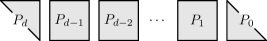
Figure 1: Structure of the matrices: $P_{d}$ upper and $P_{0}$ lower triangular

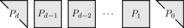
Figure 2: Structure of the matrices: $P_{d}$ and $P_{0}$ upper triangular

These structures can be achieved stably by computing the generalized Schur decomposition of either $(P_{d},P_{0}^{-*})$ or $(P_{d},P_{0})$. Suppose $U$ and $V$ are the two unitary matrices such that $U^{*}P_{d}V$ is upper triangular and $U^{*}P_{0}V$ is triangular.

Performing an equivalence transformation on (2) with $U$ and $V$ provides the desired factorization. In the remainder of this section we will therefore assume without loss of generality that all $P_{i}$’s are overwritten by $U^{*}P_{i}V$, such that the leading coefficient $P_{d}=N_{d}$ is upper triangular and the constant term $P_{0}=M_{0}$ is triangular.

2.2 Frobenius factorization

The block companion matrix $S$ from (3) having its upper right block $M_{0}$ in lower triangular form (see Figure 1) can be factored into the product of scalar companion matrices.

Theorem 1 (Frobenius factorization).

The block companion matrix $S$ in (3), with blocks $M_{i}\in{\mathbb{C}}^{k\times k}$ and $M_{0}$ lower triangular, can be factored as $S=S_{1}S_{2}\cdots S_{k}$, where each $S_{i}\in{\mathbb{C}}^{n\times n}$, $n=dk$, is the Frobenius companion matrix linked to a scalar monic polynomial of degree $n$.

Proof.

The proof is constructive and proceeds recursively. We show how to factor a companion matrix $S$ into the product of two matrices $S=S_{1}\widetilde{S}$, with $S_{1}$ a companion matrix of a scalar polynomial of degree $n=dk$ and $\widetilde{S}$ the matrix on which we will apply the recursion.

Consider $J$ the $n\times n$ nilpotent downshift matrix, i.e., it has ones on the subdiagonal and zeros elsewhere. Name $M=[M_{0}^{T},M_{1}^{T},\ldots,M_{d-1}^{T}]^{T}$ the skinny matrix of size $n\times k$ having all $M_{i}$ stacked vertically. The elements of the blocks $M_{i}$ ($0\leqslant i\leqslant d-1$) are indexed according to their position in $M$, thus $M_{0}$ and $M_{d-1}$ look like

$$\left[\begin{array}[]{cccc}m_{11}\\ m_{21}&m_{22}&\\ \vdots&&\ddots\\ m_{k1}&m_{k2}&\cdots&m_{kk}\\ \end{array}\right]\;\;\mbox{and}\;\;\left[\begin{array}[]{cccc}m_{(d-1)k+1,1}&m_{(d-1)k+1,2}&\cdots&m_{(d-1)k+1,k}\\ m_{(d-1)k+2,1}&m_{(d-1)k+2,2}&&m_{(d-1)k+2,k}\\ \vdots&&\ddots&\vdots\\ m_{dk,1}&m_{dk,2}&\cdots&m_{dk,k}\\ \end{array}\right].$$

The block companion matrix $S=J^{k}-M\left[\;0,\;\ldots,\;0,\;I_{k}\right]$ admits a factorization $S_{1}\widetilde{S}$, where $S_{1}=J-\left[m_{11},m_{21},\ldots,m_{dk,1}\right]^{T}\,e_{n}^{T}$, and $\widetilde{S}=J^{k-1}-\widetilde{M}\left[\;0,\;\ldots,\;0,\;I_{k-1}\right]\;,$ with $e_{n}$ the $n$-th standard basis vector and $\widetilde{M}$ of size $n\times(k-1)$ consisting of the last $k-1$ columns of $M$ moved up one row. The top $k$ and bottom $k$ rows of $\widetilde{M}$ are thus of the forms

$$\left[\begin{array}[]{cccc}m_{22}\\ m_{32}&m_{33}&\\ \vdots&&\ddots\\ m_{k,2}&m_{k,3}&\cdots&m_{k,k}\\ m_{k+1,2}&m_{k+1,3}&\cdots&m_{k+1,k}\\ \end{array}\right]\;\;\mbox{and}\;\;\left[\begin{array}[]{cccc}m_{(d-1)k+2,2}&m_{(d-1)k+2,3}&\cdots&m_{(d-1)k+2,k}\\ m_{(d-1)k+3,2}&m_{(d-1)k+3,3}&&m_{(d-1)k+3,k}\\ \vdots&&\ddots&\vdots\\ m_{dk,2}&m_{dk,3}&\cdots&m_{dk,k}\\ 0&0&\cdots&0\end{array}\right].$$

Continuing to factor $\widetilde{S}$ in a similar way results in the desired factorization $S=S_{1}\cdots S_{k}$, where each $S_{i}$ is the Frobenius companion linearization of a degree $n=dk$ scalar polynomial. ∎

Remark 2.

Computing the Frobenius factorization is cheap and stable as no arithmetic operations are involved.

Example 3.

Consider a degree $3$ matrix polynomial $\lambda^{3}I_{3}+\lambda^{2}M_{2}+\lambda M_{1}+M_{0}$ with $3\times 3$ blocks

$$M_{0}=-\left[\begin{array}[]{ccc}1&&\\ 2&10&\\ 3&11&18\\ \end{array}\right],\;\;M_{1}=-\left[\begin{array}[]{ccc}4&12&19\\ 5&13&20\\ 6&14&21\\ \end{array}\right],\;\;\mbox{and}\;\;M_{2}=-\left[\begin{array}[]{ccc}7&15&22\\ 8&16&23\\ 9&17&24\\ \end{array}\right].$$

The associated companion matrix $S$ equals $S_{1}S_{2}S_{3}$, with

$$\small S_{1}=\left[\begin{array}[]{cccccc}&&&&&1\\ 1&&&&&2\\ &\ddots&&&&\vdots\\ &&1&&&7\\ &&&1&&8\\ &&&&1&9\end{array}\right],\;S_{2}=\left[\begin{array}[]{ccccccc}&&&&&10\\ 1&&&&&11\\ &\ddots&&&&\vdots\\ &&1&&&16\\ &&&1&&17\\ &&&&1&0\end{array}\right],\;S_{3}=\left[\begin{array}[]{cccccc}&&&&&18\\ 1&&&&&19\\ &\ddots&&&&\vdots\\ &&1&&&24\\ &&&1&&0\\ &&&&1&0\end{array}\right].$$

In Section 2.4 we will provide an alternative factorization of the block companion matrix $S$, which, as we will show in Section 9 leads to a slightly better bound on the backward error.

2.3 Gaussian factorization

Both $S$ and $T$ are of unitary-plus-low-rank form, which is essential for developing a fast algorithm. For proving backward stability in Section 9, we need, however, more; we require that all the factors in the factorizations of $S$ and $T$ have the low rank part concentrated in a single column, the spike. For instance a companion is also a unitary-plus-spike matrix. For factoring $T$ from (3), we will use Gaussian transformations providing us a factorization into identity-plus-spike matrices, that is, matrices that can be written as the sum of the identity and a rank-one matrix having a single nonzero column.

Theorem 4 (Gaussian factorization).

The matrix $T$ from (3), with matrix blocks $N_{i}\in\mathbb{C}^{k\times k}$ and $N_{d}$ upper triangular can be factored as $T=T_{1}T_{2}\cdots T_{k}$, where each $T_{i}\in{\mathbb{C}}^{n\times n}$, with $n=dk$, is upper triangular and of identity-plus-spike form.

Proof.

The proof is again of recursive and constructive nature and involves elementary matrix operations. We will factor $T$ as $\tilde{T}T_{k}$, where $T_{k}$ is of the desired upper triangular and identity-plus-spike form, the recursion will be applied on the matrix $\tilde{T}$. Write

$$T=I_{n}+[N_{1}^{T},N_{2}^{T},\ldots,N_{d-1}^{T},\tilde{N}_{d}^{T}]^{T}[0,\ldots,0,I_{k}]=I_{n}+\tilde{N}\;[0,\ldots,0,I_{k}],$$

with $\tilde{N}\in{\mathbb{C}}^{n\times k}$ and $\tilde{N}_{d}=N_{d}-I_{k}$. Again we index the individual blocks $N_{i}$ ($1\leqslant i\leqslant d-1$) and $\tilde{N}_{d}$ according to $N$. It is easily verified that $T=\widetilde{T}T_{k}$, with

$$T_{k}=I_{n}+\left[n_{11},n_{21},\ldots,\\ \tilde{n}_{(d-1)k+1,1},\\ 0,\ldots,0\right]e_{(d-1)k+1}^{T}=(\tilde{N}e_{1})e_{(d-1)k+1}^{T},$$

and

$$\widetilde{T}=I_{n}+\left[\begin{array}[]{cccc}n_{12}&n_{13}&\cdots&n_{1k}\\ n_{22}&n_{23}&\cdots&n_{2k}\\ \vdots&\vdots&&\vdots\\ n_{(d-1)k,2}&n_{(d-1)k,3}&\cdots&n_{(d-1)k,k}\\ \tilde{n}_{(d-1)k+1,2}&\tilde{n}_{(d-1)k+1,3}&\cdots&\tilde{n}_{(d-1)k+1,k}\\ \tilde{n}_{(d-1)k+2,2}&\tilde{n}_{(d-1)k+2,3}&\cdots&\tilde{n}_{(d-1)k+2,k}\\ &\tilde{n}_{(d-1)k+3,3}&\cdots&\tilde{n}_{(d-1)k+3,k}\\ &&\ddots&\vdots\\ &&&\tilde{n}_{dk,k}\\ \end{array}\right][0_{(k-1)\times((d-1)k+1)},I_{k-1}].$$

Continuing to factor $\widetilde{T}$ proves the theorem.

∎

Remark 5.

There are two important consequences of having $P_{d}=N_{d}$ in upper triangular form. First, the proof of Theorem 4 reveals that we can compute the factorization in an exact way, as no computations are involved. Second, all factors in the factorization of $T$ are already in upper triangular form, which will come in handy in Section 5 when transforming the pencil $(S,T)$ to Hessenberg-triangular form.

Example 6.

Consider a $9\times 9$ upper triangular matrix $T$ as in (3), with $3\times 3$ blocks

$$N_{2}=\left[\begin{array}[]{ccc}1&8&16\\ 2&9&17\\ 3&10&18\end{array}\right],\quad N_{3}=\left[\begin{array}[]{ccc}4&11&19\\ 5&12&20\\ 6&13&21\\ \end{array}\right],\;\mbox{and}\;\quad N_{4}=\left[\begin{array}[]{ccc}7&14&22\\ &15&23\\ &&24\end{array}\right].$$

Then we have that $T=T_{1}T_{2}T_{3}$ with

$$\small T_{1}=\left[\begin{array}[]{cccccc}1&&&&&16\\ &\ddots&&&&\vdots\\ &&1&&&21\\ &&&1&&22\\ &&&&1&23\\ &&&&&24\end{array}\right],\;T_{2}=\left[\begin{array}[]{cccccc}1&&&&8&\\ &\ddots&&&\vdots&\\ &&1&&13&\\ &&&1&14&\\ &&&&15&\\ &&&&&1\end{array}\right],\;T_{3}=\left[\begin{array}[]{cccccc}1&&&1\\ &\ddots&&\vdots\\ &&1&6\\ &&&7&\\ &&&&1\\ &&&&&1\end{array}\right].$$

2.4 Gaussian factorization of the block companion matrix

In this section we provide a second option for factoring the block companion matrix $S$ (see (3)). Whereas Theorem 1 factors $S$ into regular Frobenius companion matrices, the factorization proposed here relies only on Theorem 4 for factoring upper triangular matrices. To be able to do so the block $M_{0}$ needs to be in upper triangular form (see Figure 2), in contrast to the lower triangular form required by Theorem 1.

Instead of factoring $S$ directly we compute its QR factorization first. Let ($n=dk$)

$$\mathcal{Q}=\left[\begin{array}[]{ccccc}0&0&\cdots&0&1\\ 1&&&&0\\ &1&&&0\\ &&\ddots&&\vdots\\ &&&1&0\end{array}\right]\in{\mathbb{C}}^{n\times n},$$ (11)

leading to

$$S=\mathcal{Q}^{k}R=\left[\begin{array}[]{ccccc}0&0&\cdots&0&I_{k}\\ I_{k}&&&&0\\ &I_{k}&&&0\\ &&\ddots&&\vdots\\ &&&I_{k}&0\end{array}\right]\left[\begin{array}[]{ccccc}I_{k}&&&&-M_{1}\\ &I_{k}&&&-M_{2}\\ &&\ddots&&\vdots\\ &&&I_{k}&-M_{d-1}\\ &&&&-M_{0}\end{array}\right].$$

The upper triangular matrix $R$ can be factored by Theorem 4 as $R=R_{1}\cdots R_{k}$, providing a factorization of $S$ of the form $S=\mathcal{Q}^{k}R_{1}\cdots R_{k}$.

3 Structured storage

To develop an efficient product eigenvalue algorithm we will exploit the structure of the factors. In addition to being sparse, all factors are also of unitary-plus-rank-one form, and we can use an $\mathcal{O}(n)$ storage scheme, where $n=dk$. We recall how to efficiently store these matrices, since the upper triangular factors differ slightly from what is presented by Aurentz et al. [1].

To factor these matrices efficiently we use core transformations $Q_{i}$, which are identity matrices except for a unitary two by two block $Q_{i}(i:i+1,i:i+1)$. Note that the subscript $i$ in core transformations will always refer to the active part $(i:i+1,i:i+1)$. For instance rotations or reflectors operating on two consecutive rows are core transformations.

Let us first focus on the factorization $S=S_{1}\cdots S_{k}$ from Section 2.2. All matrices $S_{i}$ with $1\leqslant i\leqslant k$ are of unitary-plus-rank-one and of Hessenberg form and we replace them by their QR factorization $S_{i}=\mathcal{Q}R_{i}$. This factors the companion matrices into a unitary $\mathcal{Q}$ and upper triangular identity-plus-spike matrices $R_{i}$. Indeed, the matrix $\mathcal{Q}$ is, initially, identical for all $S_{i}$, and looks like (11), being the product of $n-1$ core transformations: $\mathcal{Q}=Q_{1}\dotsm Q_{n-1}$, with all $Q_{i}(i:i+1,i:i+1)=\left[\begin{smallmatrix}0&1\\ 1&0\end{smallmatrix}\right]$ counteridentities. From now on, we will use caligraphic letters to denote a sequence of core transformations such as $\mathcal{Q}$. Because the core transformations in $\mathcal{Q}$ are ordered such that the first one acts on rows $1$ and $2$, the second one on rows $2$ and $3$, the third one on rows $3$ and $4$, and so forth, we will refer to it as a descending sequence of core transformations. When presenting core transformations pictorially as in Section 5 we see that $\mathcal{Q}$ clearly describes a descending pattern of core transformations.

As a result we have a factorization for $S$ of the form

$$\begin{array}[]{rcll}S&=&S_{1}S_{2}\cdots S_{k}\;=\;\mathcal{Q}R_{1}\,\mathcal{Q}R_{2}\,\cdots\,\mathcal{Q}R_{k}&\quad(\mbox{Frobenius factorization}).\end{array}$$ (13)

Alternatively, considering the factorization from Section 2.4, we would get

$$\begin{array}[]{rcll}S&=&\mathcal{Q}^{k}R_{1}\cdots R_{k}&\quad(\mbox{Gaussian factorization}).\end{array}$$ (14)

It is important to notice that even though (13) and (14) use the same symbols $R_{i}$, they are different. However, as both factorizations are never used simultaneously, we will reuse these symbols throughout the text.

Since $\mathcal{Q}$ can be factored into $n-1$ core transformations $\mathcal{Q}^{k}$ from (11) admits a factorization into $k$ descending sequences of core transformations too. It remains to efficiently store the upper triangular identity-plus-spike matrices $R_{i}$:

$$R_{i}=\left[\begin{array}[]{cccccccc}1&&&&\times\\ &1&&&\times\\ &&\ddots&&\vdots\\ &&&1&\times\\ &&&&\times\\ &&&&&1\\ &&&&&&\ddots\\ &&&&&&&1\end{array}\right].$$ (15)

In the Frobenius case (13) the spike is always located in the last column and in Gaussian case (14) the spike is found in column $n+1-i$.

For simplicity we drop the subscript $i$ and we deal with all cases at once: Let $R$ have the form (15), with the spike in column $\ell$. Then $R=Y+(x-e_{\ell})y^{T}$ with $Y=I_{n}$ unitary, $x\in\mathbb{C}^{n}$ the vector containing the spike, and $y=e_{\ell}\in\mathbb{C}^{n}$. We begin by embedding $R$ in a larger matrix $\underline{R}$ having one extra zero row and an extra column with only a single element different from zero:

$$\underline{R}=\left[\begin{array}[]{cccccccc|c}1&&&&\times&&&&0\\ &1&&&\times&&&&0\\ &&\ddots&&\vdots&&&&\vdots\\ &&&1&\times&&&&0\\ &&&&\times&&&&1\\ &&&&&1&&&0\\ &&&&&&\ddots&&\vdots\\ &&&&&&&1&0\\ \hline\cr 0&0&\cdots&0&0&0&\cdots&0&0\end{array}\right].$$

Let $P$ denote the $(n+1)\times n$ matrix obtained by adding a zero row to the bottom of the $n\times n$ identity matrix. Then $R=P^{T}\underline{R}P$. In fact our object of interest is $R$, but for the purposes of efficient storage we need the extra room provided by the larger matrix $\underline{R}$. The $1$ in the last column ensures that the matrix $\underline{R}$ remains of unitary-plus-spike form $\underline{R}=\underline{Y}+\underline{x}\underline{y}^{T}$, where $\underline{y}=e_{\ell}\in\mathbb{C}^{n+1}$, and $\underline{x}\in\mathbb{C}^{n+1}$ is just $x$ with a $-1$ adjoined at the bottom. Thus $P^{T}\underline{y}=y$, $P^{T}\underline{x}=x$,

$$\underline{Y}=\left[\begin{array}[]{cccccccc|c}1&&&&&&&&\\ &1&&&&&&&\\ &&\ddots&&&&&&\\ &&&1&&&&&\\ &&&&0&&&&1\\ &&&&&1&&&\\ &&&&&&\ddots&&\\ &&&&&&&1&\\ \hline\cr&&&&1&&&&0\end{array}\right]\;\;\mbox{ and }\;\;\underline{x}=\left[\begin{array}[]{c}\times\\ \times\\ \times\\ \vdots\\ \times\\ 0\\ \vdots\\ 0\\ \hline\cr-1\\ \end{array}\right].$$ (16)

Let $C_{1},\dotsc,C_{n}$ be core transformations such that $C_{1}\dotsm C_{n}\underline{x}=\alpha e_{1}$, with $|{\alpha}|=\lVert\underline{x}\rVert_{2}$. Because of the nature of $\underline{x}$, each of the core transformations $C_{\ell+1},\dotsc,C_{n}$ has the simple active part $F=\left[\begin{smallmatrix}0&1\\ 1&0\end{smallmatrix}\right]$. If we use the symbol $F_{j}$ to denote a core transformation with active part $F$, then $C_{j}=F_{j}$ for $j=\ell+1$, …, $n$. Let $\mathcal{C}=C_{1}\dotsm C_{n}$. Then we can write

$$\underline{R}=\mathcal{C}^{*}(\mathcal{C}\underline{Y}+e_{1}\underline{y}^{T}),$$

where we have absorbed the factor $\alpha$ into $y$. Let $\mathcal{B}=\mathcal{C}\underline{Y}=C_{1}\dotsm C_{n}\underline{Y}$. It is easy to check that $C_{\ell+1}\dotsm C_{n}\underline{Y}=F_{\ell+1}\dotsm F_{n}\underline{Y}=F_{\ell}F_{\ell+1}\dotsm F_{n}$. Thus $\mathcal{B}=C_{1}\dotsm C_{\ell}F_{\ell}\dotsm F_{n}$, so we can write $\mathcal{B}=B_{1}\dotsm B_{n}$, where $B_{\ell}=C_{\ell}F_{\ell}$, and $B_{j}=C_{j}$ for $j\neq\ell$. As a result we get

$$R=P^{T}C_{n}^{*}\dotsm C_{1}^{*}(B_{1}\dotsm B_{n}+e_{1}\underline{y}^{T})P=P^{T}\mathcal{C}^{*}(\mathcal{B}+e_{1}\underline{y}^{T})P.$$ (17)

The symbols $P$ and $P^{T}$ are there just to make the dimensions come out right. They add nothing to the storage or computational cost, and we often forget that they are there.

Remark 7.

It was shown in [1] that by adding an extra row and column to the matrix $R$, preserving the unitary-plus-spike and the upper triangular structure, that all the information about the rank-one part is encoded in the unitary part. Thus we will not need to store the rank-one-part explicitly. We will consider this in more detail in Section 9 when discussing the backward error.

The overall computational complexity for efficiently storing the factored form of the pencil equals $\mathcal{O}(dk^{3})$ subdivided in the following parts.

The preprocessing step to bring the constant and leading coefficient matrix to suitable triangular form requires solving a product eigenvalue problem or computing a Schur decomposition which costs $\mathcal{O}(k^{3})$ operations. Also the other matrices require updating: $2(d-1)$ matrix-matrix products, assumed to take $\mathcal{O}(k^{3})$ each are executed. Factoring $T$ and $S$ is for free since no arithmetic operations are involved. Overall, computing the factored form requires thus $\mathcal{O}(dk^{3})$ operations.

The cost of computing the efficient storage of a single identity-plus-spike matrix is essentially the one of computing $\mathcal{C}\underline{x}=\alpha e_{1}$. This requires computing $n=dk$ core transformations for $2k$ matrices. In total this sums up to $\mathcal{O}(dk^{2})$.

4 Operating with core transformations

The proposed factorizations are entirely based on core transformations; we need three basic operations to deal with them: a fusion, a turnover, and a pass-through operation. To understand the flow of the algorithm better we will explain it with pictures. A core transformation is therefore pictorially denoted as $\begin{smallmatrix}\raisebox{-3.1298pt}[2.84544pt][0.0pt]{\mbox{$\Rsh$}}\\[3.01385pt] \raisebox{3.1298pt}[2.84544pt][0.0pt]{\mbox{\rotatebox[origin={c}]{180.0}{\reflectbox{\raisebox{-3.1298pt}[2.84544pt][0.0pt]{\mbox{$\Rsh$}}}}}}\end{smallmatrix}$, where the arrows pinpoint the rows affected by the transformation.

Two core transformations $F_{i}$ and $G_{i}$ undergo a fusion when they operate on identical rows and can be replaced by a single core tranformation $H_{i}=F_{i}G_{i}$. Pictorially this is shown on the left of (18). Given a product $F_{i}G_{i+1}H_{i}$ of three core transformations, then one can always refactor the product as ${F}_{i+1}{G}_{i}{H}_{i+1}$. This operations is called a turnover. This is shown pictorially on the right of (18).

$$\begin{matrix}\raisebox{-3.1298pt}[2.84544pt][0.0pt]{\mbox{$\Rsh$}}&\raisebox{-3.1298pt}[2.84544pt][0.0pt]{\mbox{$\Rsh$}}\\ \raisebox{3.1298pt}[2.84544pt][0.0pt]{\mbox{\rotatebox[origin={c}]{180.0}{\reflectbox{\raisebox{-3.1298pt}[2.84544pt][0.0pt]{\mbox{$\Rsh$}}}}}}&\raisebox{3.1298pt}[2.84544pt][0.0pt]{\mbox{\rotatebox[origin={c}]{180.0}{\reflectbox{\raisebox{-3.1298pt}[2.84544pt][0.0pt]{\mbox{$\Rsh$}}}}}}\end{matrix}\ =\ \begin{matrix}\raisebox{-3.1298pt}[2.84544pt][0.0pt]{\mbox{$\Rsh$}}\\ \raisebox{3.1298pt}[2.84544pt][0.0pt]{\mbox{\rotatebox[origin={c}]{180.0}{\reflectbox{\raisebox{-3.1298pt}[2.84544pt][0.0pt]{\mbox{$\Rsh$}}}}}}\end{matrix}\;,\quad\quad\quad\quad\begin{matrix}\raisebox{-3.1298pt}[2.84544pt][0.0pt]{\mbox{$\Rsh$}}&&\raisebox{-3.1298pt}[2.84544pt][0.0pt]{\mbox{$\Rsh$}}\\ \raisebox{3.1298pt}[2.84544pt][0.0pt]{\mbox{\rotatebox[origin={c}]{180.0}{\reflectbox{\raisebox{-3.1298pt}[2.84544pt][0.0pt]{\mbox{$\Rsh$}}}}}}&\raisebox{-3.1298pt}[2.84544pt][0.0pt]{\mbox{$\Rsh$}}&\raisebox{3.1298pt}[2.84544pt][0.0pt]{\mbox{\rotatebox[origin={c}]{180.0}{\reflectbox{\raisebox{-3.1298pt}[2.84544pt][0.0pt]{\mbox{$\Rsh$}}}}}}\\ &\raisebox{3.1298pt}[2.84544pt][0.0pt]{\mbox{\rotatebox[origin={c}]{180.0}{\reflectbox{\raisebox{-3.1298pt}[2.84544pt][0.0pt]{\mbox{$\Rsh$}}}}}}&\\ \end{matrix}\ =\begin{matrix}&\raisebox{-3.1298pt}[2.84544pt][0.0pt]{\mbox{$\Rsh$}}&\\ \raisebox{-3.1298pt}[2.84544pt][0.0pt]{\mbox{$\Rsh$}}&\raisebox{3.1298pt}[2.84544pt][0.0pt]{\mbox{\rotatebox[origin={c}]{180.0}{\reflectbox{\raisebox{-3.1298pt}[2.84544pt][0.0pt]{\mbox{$\Rsh$}}}}}}&\raisebox{-3.1298pt}[2.84544pt][0.0pt]{\mbox{$\Rsh$}}\\ \raisebox{3.1298pt}[2.84544pt][0.0pt]{\mbox{\rotatebox[origin={c}]{180.0}{\reflectbox{\raisebox{-3.1298pt}[2.84544pt][0.0pt]{\mbox{$\Rsh$}}}}}}&&\raisebox{3.1298pt}[2.84544pt][0.0pt]{\mbox{\rotatebox[origin={c}]{180.0}{\reflectbox{\raisebox{-3.1298pt}[2.84544pt][0.0pt]{\mbox{$\Rsh$}}}}}}\\ \end{matrix}\;.$$ (18)

The final operation involves core transformations and upper triangular matrices. A core transformation can be moved from one side of an upper triangular matrix to the other side: $RG_{i}=\tilde{G}_{i}\tilde{R}$, named a pass-through operation.

When describing an algorithm with core transformations, typically one core transformation is more important than the others and it is desired to move this transformation around. Pictorally we represent the movement of a core transformation by an arrow. For instance

(19)

demonstrates pictorially the movement of a core transformation from the right to the left as the result of executing a turnover (left and middle picture of (19)) and a fusion (right picture of (19)), where the right rotation is fused with the one on the left. We need pass-through operations in both directions, pictorially shown as

In the description of the forthcoming algorithms we will also pass core transformations through the inverses of upper triangular matrices. In case of an invertible upper triangular matrix $R$, this does not pose any problems; numerically, however, this is unadvisable as we do not wish to invert $R$. So instead of computing $R^{-1}G_{i}=\tilde{G}_{i}\tilde{R}^{-1}$ we compute $G^{*}_{i}R=\tilde{R}\tilde{G}^{*}_{i}$, which can be executed numerically reliably (even when $R$ is singular). Pictorially

Not only will we pass core transformations through the inverses of upper triangular matrices, we will also pass them through sequences of upper triangular matrices. Suppose, e.g., that we have a product of $\ell$ upper triangular matrices $R_{1}\cdots R_{\ell}$ and we want to pass $G_{i}$ from the right to the left through this sequence. Passing the core transformation sequentially through $R_{\ell}$, $R_{\ell-1}$, up to $R_{1}$ provides us $(R_{1}\cdots R_{\ell})G_{i}=\tilde{G}_{i}(\tilde{R}_{1}\cdots\tilde{R}_{\ell}).$ Or, simply writing $R=R_{1}\cdots R_{\ell}$ we have $RG_{i}=\tilde{G}_{i}\tilde{R}$, what is exactly what we will often do to simplify the pictures and descriptions. Pictorially

One important issue remains. We have described how to pass a core transformation from one side to the other side of an upper triangular matrix. In practice, however, we do not have dense upper triangular matrices, but a factored form as presented in (17), which we are able to update easily. Since the rank-one part can be recovered from the unitary matrices $\mathcal{C}$ and $\mathcal{B}$, we can ignore it; passing a core transformation through the upper triangular matrix $R=P^{T}\mathcal{C}^{*}(\mathcal{B}+e_{1}\underline{y}^{T})P$ can be replaced by passing a core transformation through the unitary part $\mathcal{C}^{*}\mathcal{B}$ only. So $RG_{i}=\tilde{G}_{i}\tilde{R}$ is computed as $(\mathcal{C}^{*}\mathcal{B})\underline{G}_{i}=\underline{\tilde{G}}_{i}(\tilde{\mathcal{C}}^{*}\tilde{\mathcal{B}})$, where $\underline{G}_{i}=\left[\begin{smallmatrix}G_{i}&0\\ 0&1\end{smallmatrix}\right]$ and $\underline{\tilde{G}}_{i}=\left[\begin{smallmatrix}\tilde{G}_{i}&0\\ 0&1\end{smallmatrix}\right]$ and thus $\underline{G}_{i}P=PG_{i}$ and $\underline{\tilde{G}}_{i}P=P\tilde{G}_{i}$. The pass-through operation requires two turnovers as pictorially shown, for $d=2$, $k=3$, and $n=dk=6$,

We emphasize that $\underline{G}_{i}e_{n+1}=\underline{\tilde{G}}_{i}e_{n+1}=e_{n+1}$ and $W^{*}e_{1}=e_{1}$ will always hold and these relations are used in the backward error analysis.

All these operations, i.e., a turnover, a fusion, and a pass-through, require a constant $\mathcal{O}(1)$ number of arithmetic operations and are thus independent of the matrix size. As a result, passing a core transformation through a sequence of compactly stored upper triangular unitary-plus-rank-one matrices costs $\mathcal{O}(k)$, where $k$ is the number of upper triangular matrices involved. Moreover, the turnover and the fusion are backward stable operations [1], they introduce only errors of the order of the machine precision on the original matrices. The stability of a pass-through operation involving factored upper-triangular-plus-rank-one matrices will be discussed in Section 9.

5 Transformation to Hessenberg-triangular form

The companion matrix $S$ has $k$ nonzero subdiagonals. To efficiently compute the eigenvalues of the pencil $(S,T)$ via Francis’s implicitly shifted QR algorithm [14, 15] we need a unitary equivalence to transform the pencil to Hessenberg-triangular form.

We will illustrate the reduction procedure on the Frobenius factorization (13), though it can be applied equally well on the Gaussian factorization (14). We search for unitary matrices $U$ and $V$ such that the pencil ($U^{*}SV$, $U^{*}TV$) is of Hessenberg-triangular form. We operate directly on the factorized versions of $S$ and $T$ in $U^{*}SVV^{*}T^{-1}U$ and we compute

$$(U^{*}S_{1}U_{1})\;(U_{1}^{*}S_{2}U_{2})\;\cdots\;(U_{k-1}^{*}S_{k}V)\;(V^{*}T_{k}^{-1}V_{k-1})\;(V_{k-1}^{*}T_{k-1}^{-1}V_{k-2})\;\cdots\;(V_{1}^{*}T_{1}^{-1}U)$$

$$= \tilde{S}_{1}\;\tilde{S}_{2}\;\cdots\;\tilde{S}_{k}\;\tilde{T}_{k}^{-1}\;\tilde{T}_{k-1}^{-1}\;\cdots\;\tilde{T}_{1}^{-1},$$

where $\tilde{S}_{1}$ is Hessenberg and all other factors $\tilde{S}_{2},\ldots\tilde{S}_{k},\tilde{T}_{1},\ldots,\tilde{T}_{k}$ are upper triangular. Every time we have to pass a core transformation through an $n\times n$ upper triangular factor we use the efficient representation and the tools described in Section 4 to pass it through the product and the inverse factors.

We illustrate the procedure on a running example with $k=3$ and $d=2$, so the matrices are of size $6\times 6$ and the product is of the form

However, we do not work on these Hessenberg matrices, but directly on their QR factorizations. Pictorially, where for simplicity of presentation we have replaced $T_{3}^{-1}T_{2}^{-1}T_{1}^{-1}$ by $T^{-1}$ we get

It remains to remove all subdiagonal elements of the matrices $S_{2}$ and $S_{3}$, this means that all core transformations between matrices $R_{1}$ and $R_{2}$, and the matrices $R_{2}$ and $R_{3}$ need to be removed. We will first remove all the core transformations acting on rows $1$ and $2$, followed by those acting on rows $2$ and $3$, and so forth. We remove transformations from the right to the left, so first the top core transformation between $R_{2}$ and $R_{3}$ is removed followed by the top core transformation between $R_{1}$ and $R_{2}$.

First we bring the top core transformation in the last sequence to the outer left. The transformation has to undergo two pass-through operations: one with $R_{2}$ and one with $R_{1}$, and two turnovers to get it there

To continue the chasing a similarity transformation is executed removing the rotation from the left and bringing it to the right of the product. Pictorially

As a result we now have a core transformation on the outer right operating on rows $3$ and $4$. Originally this transformation was acting on rows $1$ and $2$. Every time we do a turnover the core transformation moves down a row. The operation of moving a core transformation to the outer left and then bringing it back to the right via a similarity transformation is vital in all forthcoming algorithms, we will name this a sweep. Depending on the number of turnovers executed in a sweep, the effect is clearly a downward move of the involved core transformation. Finally it hits the bottom and gets fused with another core transformation.

We continue this procedure and try to execute another sweep: we move the transformation on the outer right back to the outer left by $5$ pass-through operations ($3$ are needed to pass the transformation through $T^{-1}=T_{3}^{-1}T_{2}^{-1}T_{1}^{-1}$) and $2$ turnovers. At the end, the core transformation under consideration operates on the bottom two rows as it was moved down $2$ times. The result looks like

At this point it is no longer possible to move the core transformation further to the left. We can get rid of it by fusing it with the bottom core transformation of the first sequence. We have removed a single core transformation and it remains to chase the others in a similar fashion. Pictorially we have

The top core transformation in the second sequence is now marked for removal. Pictorially we have accumulated all steps leading to

The next core transformation to be chased is the second one of the outer right sequence of core transformations we are handling. Pictorially all steps of the chasing at once look like

The entire procedure to chase a single core transformation consists of executing sweeps until the core transformation hits the bottom and can fuse with another core transformation.

At the very end we obtain the factorization

(20)

This matrix is in upper Hessenberg form and on this factorization we will run the product eigenvalue problem.

The algorithm annihilates the unwanted core transformations acting on the first rows, followed by those acting on the second row, and so forth. As a consequence a single full sweep from right to left always takes $k$ turnovers and $2k$ pass-through operations, and gets thus a complexity $\mathcal{O}(k)$. To get rid of a single core transformation $G_{i}$ we need approximately $\lfloor(dk-i)/k\rfloor$ sweeps leading to an approximate complexity count

$$\sum_{i=1}^{dk}\sum_{j=1}^{k-1}\frac{dk-i}{k}k=\mathcal{O}(d^{2}k^{3}),$$

where $i$ runs over the core transformations and $j$ over the sequences.

6 Product eigenvalue problem

The following discussion is a concise description of the actual QR algorithm. It is based on the results of Aurentz, Mach, Vandebril, and Watkins [1, 29] combined with Watkins’s interpretation of product eigenvalue problems [30]. For simplicity, we will only describe a single shifted QR step in the Hessenberg case, for information beyond the Hessenberg case we refer to Vandebril [28].

Suppose we have a Hessenberg-triangular pencil $(\tilde{S},\tilde{T})$, with $\tilde{S}=\tilde{S}_{1}\cdots\tilde{S}_{k}$ and $\tilde{T}=\tilde{T}_{1}\cdots\tilde{T}_{k}$, where $\tilde{S}_{1}$ is of Hessenberg form and all other factors upper triangular and nonsingular. The algorithm for solving the generalized product eigenvalue problem can be seen as a QR algorithm applied on $\tilde{S}\tilde{T}^{-1}$. Pictorially, for $d=2$, $k=3$, and $n=dk=6$, this looks as in (20). As before all upper triangular factors are combined into a single one, where $\tilde{S}_{1}=\tilde{Q}_{1}\tilde{R}_{1}$ is a QR factorization of $\tilde{S}_{1}$. Pictorially we get

To initiate the core chasing algorithm we pick a suitable shift $\mu$ and form $u=(\tilde{S}-\mu\tilde{T})e_{1}$. The initial similarity transformation is determined by the core transformation $U_{1}$ such that $U_{1}^{*}u=\alpha e_{1}$ for some $\alpha$. We fuse the two outer left core transformations and pass the core transformation $U_{1}$ on the right through the upper triangular matrix to get a new core transformation $X_{1}$. Pictorially we get the left of (21). The resulting matrix is not of upper Hessenberg form anymore, it is perturbed by the core transformation $X_{1}$. We will chase this core transformation to the bottom. We name this core transformation $X_{1}$ the misfit. A turnover will move $X_{1}$ to the outer left. Pictorially we get the right of (21).

                (21)

Next we execute a similarity transformation with $U_{2}$. This will cancel out $U_{2}$ on the left and bring it to the right. Next pass $U_{2}$ through the upper triangular matrix. Pictorially the flow looks like the left of (22). This looks similar to (21), except for the misfit which has moved downward one row. We can continue now by executing a turnover, a similarity, and a pass-through to move the misfit down one more position. Pictorially we end up in the right of (22).

                (22)

After $n-2$ similarities we are not able to execute a turnover anymore. The final core transformation $X_{n-1}$ fuses with the last core transformation of the sequence and we are done

In fact we continue executing sweeps until the core transformation hits the bottom and gets fused. After few QR steps a deflation will occur. Classically a deflation in a Hessenberg matrix is signaled by subdiagonal elements being relatively small with respect to the neighbouring diagonal elements. Before being able to utilize this convergence criterion we would need to compute and accumulate all diagonal elements of the compactly stored upper triangular factors. In this factored form, however, a cheaper and more reliable [21] criterion is more suitable. Deflations are signaled by almost diagonal core transformations in the descending sequence preceding the upper triangular factors. Only a simple check of the core transformations is required and we do not need to extract the diagonal elements out the compact representation, nor do we need to accumulate them.

Solving the actual product eigenvalue problem requires to compute $n=dk$ eigenvalues, where on average each eigenvalue should be found in a few QR steps. A single QR step requires the chasing of an artificially introduced core transformation. During each sweep this core transformation moves down a row because of a single turnover, hence $n=dk$ sweeps are required, each taking $2k$ pass-throughs and one turnover operations. In total this amounts to $\mathcal{O}(d^{2}k^{3})$.

7 Removing infinite and zero eigenvalues

Typically the unitary-plus-spike matrices in the factorizations will be nonsingular, but there are exceptions. If the pencil has a zero eigenvalue, then $S$ will be singular, and therefore one of the factors $R_{i}$ will necessarily be singular. If there is an infinite eigenvalue, $T$ will be singular, so one of the factors $T_{i}$ must be singular. We must therefore ask whether singularity of any of these factors can cause any difficulties.

As we shall see, infinite eigenvalues present no problems. They are handled automatically by our algorithm. Unfortunately we cannot say the same for zero eigenvalues. For the proper functioning of the Francis QR iterations, any exactly zero eigenvalues must be detected and deflated out beforehand. We will present a procedure for doing this.

7.1 Singular unitary-plus-rank-one matrices

We begin by characterizing singularity of a unitary-plus-spike factor. Suppose $R=R_{i}$ (15) is singular. (The same considerations apply to $T_{i}$.) There must be a zero on the main diagonal, and this can occur only at the intersection of the diagonal and the spike, i.e. at position $(\ell,\ell)$, where $\ell=n+1-i$. $R$ is stored in the factored form $R=P^{T}C_{n}^{*}\cdots C_{1}^{*}(B_{1}\ldots B_{n}+e_{1}y^{T})P$. The validity of this representation was established in [1], and it remains valid even though $R$ is singular. Let’s see how singularity shows up in the representation.

Recall from the construction of $\mathcal{C}$ and $\mathcal{B}$ that $C_{\ell+1},\ldots,C_{n}$, all have active part $\left[\begin{smallmatrix}0&1\\ 1&0\end{smallmatrix}\right]$. In other words $C_{j}=F_{j}$ for $j=\ell+1$, …, $n$. But now the additional zero element at position $\ell$ in $\underline{x}$ implies that also $C_{\ell}=F_{\ell}$ as well. But then $B_{\ell}=C_{\ell}F_{\ell}=F_{\ell}^{2}=I$. The converse holds as well: $B_{\ell}$ is trivial if and only if $R$ has a zero at the $\ell$th diagonal position. All of the other $B_{j}$ are equal to $C_{j}$, and these are all nontrivial.

This is the situation at the time of the initial construction of $R$. In the course of the reduction algorithm and subsequent Francis iterations, $R$ is modified repeatedly by having core transformations passed through it, but it continues to be singular and it continues to contain one trivial $B_{i}$ core transformation, as Theorem 8 below demonstrates. As preparation for this theorem we remark that Theorems 4.2, 4.3, and 4.7 of [1] remain valid, ensuring that all of the $C_{i}$ remain nontrivial.

Theorem 8 (Modification of [1, Theorem 4.3]).

Consider a factored unitary-plus-rank-one matrix $R=P^{T}\mathcal{C}^{*}(\mathcal{B}+e_{1}y^{T})P=P^{T}C_{n}^{*}\cdots C_{1}^{*}(B_{1}\cdots B_{n}+e_{1}y^{T})P$, with core transformations $C_{1}$, …, $C_{n}$ nontrivial. Then $R$ is upper triangular. Moreover $B_{\ell}$ is trivial if and only if the $\ell$th diagonal element of $R$ equals zero.

Proof.

Originally we started out with

$$\underline{R}=\left[\begin{array}[]{cc}R&\times\\ 0&0\end{array}\right]$$ (23)

where the symbol $\times$ represents a vector that is not of immediate interest. The bottom row of $\underline{R}$ is zero initially and it remains zero forever. This is so because the core transformations that are passed into and out of $R$ act on rows and columns $1$, …, $n$; they do not alter row $n+1$. Letting $H=B+e_{1}y^{T}$, we have $\underline{R}=\mathcal{C}^{*}H$, or equivalently $H=\mathcal{C}\underline{R}$. Partition this equation as

$$\left[\begin{array}[]{cc}\times&\times\\ \tilde{H}&\times\end{array}\right]=\left[\begin{array}[]{cc}\times&\times\\ \tilde{C}&\times\end{array}\right]\left[\begin{array}[]{cc}R&\times\\ 0&0\end{array}\right],$$ (24)

where $\tilde{H}$ and $\tilde{C}$ are $n\times n$ and the vectors marked $\times$ are not of immediate interest. We deduce that

$$\tilde{H}=\tilde{C}R.$$

$H$ is upper Hessenberg, so $\tilde{H}$ is upper triangular. Since all $C_{i}$ are nontrivial, $\mathcal{C}$ is a proper upper Hessenberg matrix ($c_{i+1,i}\neq 0$, $i=1,\ldots,n$), so $\tilde{C}$ is upper triangular and nonsingular. We have

$$R=\tilde{C}^{-1}\tilde{H}.$$ (25)

so $R$ must be upper triangular. Now looking at the main diagonal of the equation $\tilde{H}=\tilde{C}R$, we find that $h_{\ell+1,\ell}=c_{\ell+1,\ell}\,r_{\ell,\ell}$. Since $c_{\ell+1,\ell}\neq 0$ we see that $r_{\ell,\ell}=0$ if and only if $h_{\ell+1,\ell}=0$, and this happens if and only if $B_{\ell}$ is trivial. ∎

The existence of trivial core transformations in the factors presents no difficulties for the reduction to Hessenberg-triangular form. In some cases it will result in trivial core transformations being chased forward, but this does no harm. Now let us consider what happens in the iterative phase of the procedure.

7.2 Infinite eigenvalues

Behavior of infinite eigenvalues under Francis iterations is discussed in [31]. There it is shown that a zero on the main diagonal of $T$ gets moved up by one position on each iteration. Let’s see how this manifests itself in our structured case. Consider an example of a singular $T_{i}$ with a trivial core transformation in the third position, $B_{3}=I$, as shown pictorially below. Since $T_{i}$ is in the “inverted” part, core transformations pass through it from left to right. Suppose we pass $G_{2}$ through $T_{i}$, transforming $G_{2}T_{i}$ to $\tilde{T}_{i}\tilde{G}_{2}$. The first turnover is routine, but in the second turnover there is a trivial factor: $F_{3}B_{2}B_{3}=F_{3}B_{2}I$. This turnover is thus trivial: $F_{3}B_{2}I=IF_{3}B_{2}$. $I$ becomes the new $B_{2}$. The old $B_{2}$ is pushed out of the sequence to become $\tilde{G}_{2}$. Pictorially

The trivial core transformation in $\mathcal{B}$ has moved up one position.

On each iteration it moves up one position until it gets to the top. At that point an infinite eigenvalue can be deflated at the top. The deflation happens automatically; no special action is necessary.

7.3 Zero eigenvalues

In the case of a zero eigenvalue, one of the $R_{i}$ factors has a trivial core transformation, for example, $B_{3}$. During the iterations, core transformations pass through $R_{i}$ from right to left. One might hope that the trivial core transformation gets pushed downward by one position on each iteration, eventually resulting in a deflation at the bottom. Unfortunately this is not what happens. When a transformation $G_{2}$ is pushed into $R_{i}$ from the right, the first turnover is trivial: $B_{2}IG_{2}=I\tilde{B}_{2}I$, where $\tilde{B}_{2}=B_{2}G_{2}$. A trivial core transformation is ejected on the left, and the iteration dies.

It turns out that this problem is not caused by the special structure of our factors but by the fact that we are storing the matrix in $QR$-decomposed form. There is a simple general remedy. Consider a singular upper-Hessenberg $A$ with no special structure, stored in the form $A=Q_{1}\cdots Q_{n-1}R$. If $A$ is singular, then so is $R$, so $r_{ii}=0$ for some $i$. The reader can easily check that if $r_{ii}=0$ for $i<n$, then $a_{i+1,i}=0$, so $A$ is not properly upper Hessenberg, and a deflation should be possible. We will show how to do this below, but first consider the case when $r_{nn}=0$. We have

$$A\ =\ QR\ =\ \parbox{133.72786pt}{ \leavevmode\immediate\hbox{{\leavevmode\includegraphics{}{}{tikz/Paper-figure23.pdf}}} },$$

where $R$ has a zero at the bottom. Do a similarity transformation that moves the entire matrix $Q$ to the right. Then pass the core transformations back through $R$, and notice that when $Q_{n-1}$ is multiplied into $R$, it acts on columns $n-1$ and $n$ and does not create a bulge. Thus nothing comes out on the left. Or, if you prefer, we can say that $\hat{Q}_{n-1}=I$ comes out on the left:

$$\parbox{125.19194pt}{ \leavevmode\immediate\hbox{{\leavevmode\includegraphics{}{}{tikz/Paper-figure24.pdf}}} }\ =\ \parbox{133.72786pt}{ \leavevmode\immediate\hbox{{\leavevmode\includegraphics{}{}{tikz/Paper-figure25.pdf}}} }.$$

Now we can deflate out the zero eigenvalue.

It is easy to relate what we have done here to established theory. It is well known [31] that if there is a zero eigenvalue, one step of the explicit QR algorithm with zero shift ($A=QR$, $RQ=\hat{A}$) will extract it. This is exactly what we have done here. One can equally well check that if one does a single Francis iteration with shift $\rho=0$, this is exactly what results.

Now consider the case $r_{ii}=0$, $i<n$. Depicting the case $i=3$ we have

$$A\ =\ QR\ =\ \parbox{133.72786pt}{ \leavevmode\immediate\hbox{{\leavevmode\includegraphics{}{}{tikz/Paper-figure26.pdf}}} }.$$

Pass $Q_{i+1}$, …, $Q_{n-1}$ from left to right through $R$ to get them out of the way:

$$\parbox{150.79968pt}{ \leavevmode\immediate\hbox{{\leavevmode\includegraphics{}{}{tikz/Paper-figure27.pdf}}} }.$$

Since these do not touch row or column $i$, the zero at $r_{ii}$ is preserved. Now the way is clear to multiply $Q_{i}$ into $R$ without creating a bulge. This gets rid of $Q_{i}$. Now the core transformations that were passed through $R$ can be returned to their initial positions either by passing them back through $R$ or by doing a similarity transformation. Either way the result is

$$\parbox{133.72786pt}{ \leavevmode\immediate\hbox{{\leavevmode\includegraphics{}{}{tikz/Paper-figure28.pdf}}} },$$

or more compactly

$$\parbox{108.12054pt}{ \leavevmode\immediate\hbox{{\leavevmode\includegraphics{}{}{tikz/Paper-figure29.pdf}}} }.$$

The eigenvalue problem has been decoupled into two smaller eigenvalue problems, one of size $i\times i$ at the top and one of size $(n-i)\times(n-i)$ at the bottom. The upper problem has a zero eigenvalue, which can be deflated immediately by doing a similarity transformation with $Q_{1}\cdots Q_{i-1}$ and passing those core transformations back through $R$ as explained earlier. The result is

$$\parbox{108.12054pt}{ \leavevmode\immediate\hbox{{\leavevmode\includegraphics{}{}{tikz/Paper-figure30.pdf}}} }.$$

We now have an eigenvalue problem of size $(i-1)\times(i-1)$ at the top, a deflated zero eigenvalue in position $(i,i)$, and an eigenvalue problem of size $(n-i)\times(n-i)$ at the bottom.

We have described the deflation procedure in the unstructured case, but it can be applied equally well in the structured context of this paper. Instead of a simple upper-triangular $R$, we have a more complicated $RT^{-1}$, which is itself a product of many factors. The implementation details are different, but the procedure is the same.

8 Computation of eigenvectors

In practice typically only the left or the right eigenvectors are required. We will compute left eigenvectors since these ones are easier to retrieve than the right ones. If the right eigenvectors are wanted, one can compute the left ones of $P(\lambda)^{T}$.

For $w$ as a left eigenvector corresponding to the eigenvalue $\lambda$, i.e., $w^{T}P(\lambda)=0$, we get that

$$\hat{w}=\begin{bmatrix}w\\ \lambda w\\ \vdots\\ \lambda^{d-1}w\\ \end{bmatrix},$$

will be a left eigenvector of the companion pencil (1). This implies that once an eigenvector $\hat{w}$ of the companion pencil is computed, the first $k$ elements of that vector define the eigenvector $w$ of the matrix polynomial. To save storage and computational cost it suffices thus to compute only the first $k$ elements of each eigenvector. For reasons of numerical stability, however, we will also compute the last $k$ elements of $\hat{w}$ and use its top $k$ elements if $|\lambda|\leqslant 1$ and its trailing $k$ elements if $|\lambda|>1$ to define $w$.

Suppose our algorithm has run to completion and we have ended up with the Schur form $U^{*}(S-\lambda T)V=\hat{S}-\lambda\hat{T}$, where both $\hat{S}$ and $\hat{T}$ are upper triangular. The left eigenvector, corresponding to the eigenvalue $\hat{\lambda}$ found in the lower right corner of $\hat{S}-\lambda\hat{T}$ equals $\hat{w}=Ue_{n}$. But since the top or bottom $k$ elements of $\hat{w}$ suffice to retrieve $w$ we only need to store the top $k$ and bottom $k$ rows of $U$. Let $P$ be of size $2k\times dk$

$$P=\left[\begin{array}[]{ccccc}I_{k}&0&\ldots&0&0\\ 0&0&\ldots&0&I_{k}\end{array}\right],$$

then we see that $PUe_{n}$ provides us all essential information. As the matrix $U^{*}$ is an accumulation of all core transformations applied to the left of $S$ and $T$ during the algorithm we can save computations by forming $PU$ directly instead of $U$.

Let us estimate the cost of forming $PU$. Applying a single core transformation from the right to a $2k\times dk$ matrix costs $\mathcal{O}(k)$ operations. Each similarity transformation with a core transformation requires us to update $PU$; it remains thus to count the total number of similarities executed. In the initial reduction procedure to Hessenberg-triangular form we need at most $d$ similarities to remove a single core transformation. As roughly $dk$ core transformations need to be removed, we end up with $\mathcal{O}(d^{2}k)$ similarities. Under the assumption that a $\mathcal{O}(1)$ of QZ steps are required to get convergence to a single eigenvalue we have $\mathcal{O}(dk)$ similarities for a single eigenvalue, in total this amounts $\mathcal{O}(d^{2}k^{2})$ similarities for all eigenvalues. In total forming the matrix $PU$ has a complexity of $\mathcal{O}(d^{2}k^{3})$.

Unfortunately the Schur form allows us only to compute the left eigenvector corresponding to the eigenvalue found in the lower right corner. To compute other eigenvectors we need to reorder the Schur form so that each corresponding eigenvalue appears once at the bottom, after which we can extract the corresponding eigenvector. To reorder the Schur pencil we can rely on classical reordering methods [31]. In our setting we will only swap two eigenvalues at once and we will use core transformations to do so. To compute the core transformation that swaps two eigenvalues in the Schur pencil, we need the diagonal and superdiagonal elements of $\hat{S}$ and $\hat{T}$, these are obtained by computing the diagonal and superdiagonal elements of each of the involved factors. We refer to Aurentz et al. [1] for details on computing diagonal and superdiagonal elements of a properly stored unitary-plus-rank-one matrix. After this core transformation is computed we apply it the Schur pencil and update all involved factors by chasing the core transformation through the entire sequence. After the core transformation has reached the other end it is accumulated in $PU$.

If all eigenvectors are required, we need quite some swaps and updating. Let us estimate the cost. Bringing the eigenvalue in the bottom right position to the upper left top thereby moving down all other eigenvalues a single time requires $dk-1$ swaps. Doing this $dk-1$ times makes sure that each eigenvalue has reached the bottom right corner once, enabling us to extract the corresponding eigenvector. In total $\mathcal{O}(d^{2}k^{2})$ swaps are thus sufficient to get all eigenvectors. A single swap requires updating the $2k$ upper triangular factors involving $4k$ turnovers. Also $PU$ needs to be updated and this takes $\mathcal{O}(k)$ operations as well. In total this leads to an overall complexity of $\mathcal{O}(d^{2}k^{3})$ for computing all the eigenvectors of the matrix polynomial.

9 Backward stability

The algorithm consists of three main steps: a preprocessing of the matrix coefficients, the reduction to Hessenberg-triangular form, and the actual eigenvalue computations. We will quantify how the backward errors can accumulate in all steps. The second and third step are dealt with simultaneously. In this section we use $\doteq$ to denote an equality where some second or higher order terms have dropped, $\delta X$ will denote a perturbation of $X$, and $\lesssim$ stands for less than, up to multiplication with polynomial in $d$ and $k$ of modest degree. For simplicity we assume the norms to be unitarily invariant.We make use of the Frobenius norm, but will denote it simply as $\|\cdot\|$ without subscripted F.

The preprocessing step brings the matrix polynomial’s leading and trailing coefficients to triangular form and all other polynomial coefficients are transformed via a unitary equivalence $\tilde{P}_{i}=U^{*}P_{i}V$. In floating point arithmetic, however, we get $\hat{P}_{i}$. Relying on the backward stability of the QZ algorithm and since both $U$ and $V$ are unitary we get that $\hat{P}_{i}=U^{*}(P_{i}+\delta P_{i})V$, where $\|\delta P_{i}\|/\|P_{i}\|\lesssim u$, where $u$ denotes the unit round-off [18]. Factoring the pencil matrices is free of errors and provides us unitary-plus-spike matrices

In Section 9.1 we analyze unitary-plus-spike matrices and see that we end up with a highly structured backward error. In Sections 9.2 and 9.3 we consider the combined error of the reduction and eigenvalue computations for the Frobenius and Gaussian factorizations. We prove and show in the numerical experiments, Section 10, that both factorizations have the error bounded by the same order of magnitude, but the Gaussian factorization has a smaller constant. In Section 9.4 we conclude by formulating generic perturbation theorems pushing the error back on the pencil and on the matrix polynomial. We show that with an appropriately scaling we end up with a backward stable algorithm.

9.1 Perturbation results for unitary-plus-spike matrices

We first state a generic perturbation theorem for upper triangular unitary-plus-spike matrices. This theorem is more detailed compared to our previous error bound [1]. The precise location of the error is essential in properly accumulating the errors of the various factor matrices in Theorems 11 and 13. We show that the backward error on an upper triangular unitary-plus-spike matrix that has undergone some pass-through operations is distributed non-smoothly. Suppose the spike has zeros in the last $\ell$ spots. Then the associated upper triangular matrix will have its lower $\ell$ rows perturbed only by a modest multiple of the machine precision. The other upper rows will incorporate a larger error depending on $\|R\|$, and the upper part of the spike absorbs the largest error being proportional to $\|R\|^{2}$.

Theorem 9.

Let $R$ be an $n\times n$ upper triangular identity-plus-spike matrix factored as

$$R=P^{T}\mathcal{C}^{*}(\mathcal{B}+e_{1}\underline{y}^{T})P=I_{n}+(x-e_{\ell})y^{T},\qquad\lVert C^{*}e_{1}\rVert=\lVert\underline{x}\rVert=1,$$

with the notational conventions on $x$, $y$, $\underline{x}$, and $\underline{y}$ and the rank-one part implicitly encoded in the unitary part as in Section 3. Let $U$ and $V$ be unitary matrices representing the action of several pass-through operations through $R$ such that the resulting $\tilde{R}=U^{*}RV$ is an upper triangular unitary-plus-rank-one matrix. If $\hat{R}$ is the result obtained computing $\tilde{R}$ in floating point, operating on the unitary part only (see Section 4) and reconstructing the rank-one part from the unitary part, we get

$$\hat{R}=U^{*}(R+\delta R)V=U^{*}(R_{u}+\delta R_{u}+R_{o}+\delta R_{o})V,$$

where $R_{u}=P^{T}\mathcal{C}^{*}\mathcal{B}P$ and $R_{o}=P^{T}\mathcal{C}^{*}e_{1}\underline{y}^{T}P$, and $\delta R_{u}$ stands for the error in the unitary and $\delta R_{o}$ in the rank-one part. The error in the unitary part $\lVert\delta R_{u}\rVert\lesssim u$, and the error in the rank-one part

$$\delta R_{o}\doteq-\delta\rho_{r}\,xy^{T}+\delta w_{1}\,y^{T}+x\,\delta w_{2}^{T},$$

with $\lVert\delta w_{1}\rVert\lesssim u$, $\lVert\delta w_{2}\rVert\lesssim\lVert\underline{y}\rVert u$, and $|\delta\rho_{r}|\lesssim\lVert\underline{y}\rVert u$.

Proof.

The rank-one part of $R$ is stored implicitly in the unitary matrices so, in practice, the equivalence transformation $U^{*}RV$ only manipulates the unitary part $\mathcal{C}^{*}\mathcal{B}$. So we execute $\underline{U}^{*}\mathcal{C}^{*}\mathcal{B}\underline{V}$ where, following our notational convention, $\underline{U}=\left[\begin{smallmatrix}U&0\\ 0&1\end{smallmatrix}\right]$ and $\underline{V}=\left[\begin{smallmatrix}V&0\\ 0&1\end{smallmatrix}\right]$. This operation is implemented as $\underline{U}^{*}\mathcal{C}^{*}W\;W^{*}\mathcal{B}\underline{V}$, first passing core transformations through $\mathcal{B}$ and then through $\mathcal{C}$. The resulting upper triangular $\tilde{R}$ can therefore be factored as

$$\tilde{R}=P^{T}\underline{\tilde{R}}P=P^{T}\tilde{\mathcal{C}}^{*}(\tilde{\mathcal{B}}+e_{1}\tilde{\underline{y}}^{T})P,$$

where

$$\tilde{\mathcal{C}}=W^{*}{\mathcal{C}}\underline{U}, \tilde{\mathcal{B}}=W^{*}{\mathcal{B}}\underline{V}.$$

Letting $\tilde{\rho}=(e_{n+1}^{T}\tilde{\mathcal{C}}^{*}e_{1})$, the vector $\tilde{y}$ is given by

$$\underline{\tilde{y}}^{T} = -(e_{n+1}^{T}\tilde{\mathcal{C}}^{*}e_{1})^{-1}(e_{n+1}^{T}\tilde{\mathcal{C}}^{*}\tilde{\mathcal{B}})=-\tilde{\rho}^{-1}(e_{n+1}^{T}\tilde{\mathcal{C}}^{*}\tilde{\mathcal{B}}).$$

Since $We_{1}=e_{1}$ and $\underline{U}e_{n+1}=e_{n+1}$ we have that $\tilde{\rho}=e_{n+1}^{T}{\tilde{\mathcal{C}}}^{*}e_{1}=e_{n+1}^{T}{\mathcal{C}}^{*}e_{1}=\rho$, which in turn is the final element of $\underline{x}$.

In floating point, however, we end up with $\hat{R}$ rebuilt from the computed $\hat{\mathcal{C}}$ and $\hat{\mathcal{B}}$, which are the perturbed version of $\tilde{\mathcal{C}}$ and $\tilde{\mathcal{B}}$, by using

$$\hat{R}=P^{T}\underline{\hat{R}}P=P^{T}\hat{\mathcal{C}}^{*}(\hat{\mathcal{B}}+e_{1}\hat{\underline{y}}^{T})P,$$

where, for $\hat{\rho}=(e_{n+1}^{T}\hat{\mathcal{C}}^{*}e_{1})$, the vector $\hat{y}$ is computed from

$$\underline{\hat{y}}^{T}=-(e_{n+1}^{T}\hat{\mathcal{C}}^{*}e_{1})^{-1}(e_{n+1}^{T}\hat{\mathcal{C}}^{*}\hat{\mathcal{B}})=-\hat{\rho}^{-1}(e_{n+1}^{T}\hat{\mathcal{C}}^{*}\hat{\mathcal{B}}).$$

The matrices $\hat{\mathcal{C}}$ and $\hat{\mathcal{B}}$ are the result of executing turnovers on $\mathcal{C}$ and $\mathcal{B}$. Each turnover introduces a small backward error of the order $u$ [1] and we have, for $\lVert\delta\mathcal{C}\rVert\lesssim u$, $\lVert\delta\mathcal{B}\rVert\lesssim u$, the relations $\hat{\mathcal{C}}=W^{*}({\mathcal{C}}+\delta{\mathcal{C}})\underline{U}$ and $\hat{\mathcal{B}}=W^{*}({\mathcal{B}}+\delta{\mathcal{B}})\underline{V}$. All the individual perturbations are accumulated in $\delta{\mathcal{C}}$ and $\delta{\mathcal{B}}$, which could be dense, unstructured, in general. It’s worth noting, however, that the implementation ensures that $\hat{\mathcal{C}}$ as well as $\hat{\mathcal{B}}$ remain unitary.

Let us focus now on the factor $\hat{\rho}$. In floating point we compute $\hat{\rho}=\rho+\delta\rho_{a}=\rho(1+\delta\rho_{r})$ (subscripts $a$ and $r$ denoting the absolute and relative error respectively). Given that $|\delta\rho_{a}|\lesssim u$ we have $|\delta\rho_{r}|\lesssim|\rho|^{-1}u$, which can be bounded by $|\delta{\rho_{r}}|\lesssim\lVert\underline{y}\rVert u$. Under the assumption that $\delta\rho_{r}$ is tiny we get $(1+\delta\rho_{r})^{-1}\doteq(1-\delta\rho_{r})$.

Combining these relations and using $We_{1}=e_{1}$ and $\underline{U}e_{n+1}=e_{n+1}$ leads to

$$\underline{\hat{R}} = \underline{U}^{*}(\mathcal{C}+\delta\mathcal{C})^{*}W\;\Big{(}W^{*}(\mathcal{B}+\delta\mathcal{B})\underline{V}$$

$$\quad+e_{1}(-\rho^{-1})(1+\delta\rho_{r})^{-1}(e_{n+1}^{T}\underline{U}^{*}(\mathcal{C}+\delta\mathcal{C})^{*}W\;W^{*}(\mathcal{B}+\delta\mathcal{B})\underline{V})\Big{)}$$

$$\doteq \underline{U}^{*}\Big{(}(\mathcal{C}+\delta\mathcal{C})^{*}(\mathcal{B}+\delta\mathcal{B})-(\mathcal{C}+\delta{\mathcal{C}})^{*}e_{1}\rho^{-1}(1-\delta\rho_{r})e_{n+1}^{T}(\mathcal{C}+\delta\mathcal{C})^{*}(\mathcal{B}+\delta\mathcal{B})\Big{)}\underline{V}.$$

Using $\underline{x}=\mathcal{C}^{*}e_{1}$ and $\underline{y}^{T}=-\rho^{-1}(e_{n+1}^{T}\mathcal{C}^{*}\mathcal{B})$ provides the following approximation of the error

$$U(\hat{R}-\tilde{R})V^{*} \doteq P^{T}\Big{(}\delta{\mathcal{C}}^{*}\,{\mathcal{B}}+{\mathcal{C}}^{*}\,\delta{\mathcal{B}}+\delta{\mathcal{C}}^{*}e_{1}\underline{y}^{T}-\delta\rho_{r}\,\underline{x}\underline{y}^{T}-\rho^{-1}\underline{x}e_{n+1}^{T}(\delta{\mathcal{C}}^{*}\,\mathcal{B}+{\mathcal{C}}^{*}\,\delta\mathcal{B})\Big{)}P$$

$$=\delta R_{u}+\delta w_{1}\,y^{T}-\delta\rho_{r}\,xy^{T}+x\,\delta w_{2}^{T},$$

where $\delta R_{u}=P^{T}\left(\delta{\mathcal{C}}^{*}\,{\mathcal{B}}+{\mathcal{C}}^{*}\,\delta{\mathcal{B}}\right)P$. The bounds on the norms of $\delta w_{1}$ and $\delta w_{2}$ follow directly. ∎

We can show that $\lVert\underline{y}\rVert\leqslant\lVert\underline{R}\rVert\leqslant 1+\lVert\underline{y}\rVert$ and $\lVert R\rVert\leqslant\lVert\underline{R}\rVert\leqslant 1+\lVert R\rVert$. Looking at the four terms that comprise the backward error, we see that $\|\delta R_{u}\|\lesssim u$, $\lVert\delta w_{1}\,y^{T}\rVert\lesssim\lVert y\rVert u\lesssim\lVert R\rVert u$, $\lVert\delta\rho_{r}xy^{T}\rVert\lesssim\lVert y\rVert^{2}u\lesssim\lVert R\rVert^{2}u$, and $\lVert x\,\delta w_{2}^{T}\rVert\lesssim\lVert y\rVert u\lesssim\lVert R\rVert u$. We can conclude that $\|\delta R\|\lesssim\|R\|^{2}u$.

Note, however, that only one of the four terms has a $\lVert R\rVert^{2}$ factor, namely $\delta\rho_{r}xy^{T}$. This is a backward error; the rank-one matrix $xy^{T}$ is the initial rank-one matrix, which is in the shape of the initial spike. It follows that the part of the backward error that depends on $\lVert R\rVert^{2}$ is confined to the spike. The regions of dependence can be depicted as follows.

9.2 Gaussian factorization

We first consider the Gaussian factorization, and we write $S$ and $T$ as

$$S=QR_{1}\cdots R_{k},\mbox{ and }T=T_{1}\cdots T_{k}.$$

The structure of $T$ is a particular case of the one of $S$ where we have chosen $Q=I_{n}$. Besides $Q$ both matrices consist of a product of unitary-plus-spike matrices, and we will use the perturbation results from Theorem 9 for each of these factors individually. For simplicity we perform the backward error analysis on $S$ only. The same holds unchanged for $T$ by ignoring $Q$.

At the end of the algorithm, when $S$ has reached upper triangular form, we will have $\tilde{S}=U^{*}SV$. In floating point we compute a matrix $\hat{S}$ such that $\hat{S}=U^{*}(S+\delta S)V$. In the Gaussian case we have that, for $j=1,\ldots,k$,

$$R_{j}=I_{n}+(x_{j}-e_{\ell})y_{j}^{T},\qquad y_{j}=\alpha_{j}e_{\ell},$$ (27)

$\ell=n-j+1$. Only the first $\ell$ elements of $x_{j}$ can be different from zero. We remark that $x_{j}$ is normalized such that its enlarged version has norm one: $\|\underline{x}_{j}\|=1$. We are interested in bounding the norm of $\delta S$. A simple lemma is required, before stating the main result of the section.

Lemma 10.

For $j=1,\ldots,k$ and $R_{j}$ the factors of the Gaussian factorization (27) we have that $R_{1}\cdots R_{j-1}x_{j}=x_{j}$ and $y_{j}^{T}R_{j+1}\cdots R_{k}=y_{j}^{T}$.

Proof.

Whenever $i<j$, we have $y_{i}^{T}x_{j}=\alpha_{i}e_{n-i+1}^{T}x_{j}=0$, because of the zero structure of $x_{j}$. The relation $R_{1}\cdots R_{j-1}x_{j}=x_{j}$ follows from (27). Similar arguments prove the second relation.

∎

Theorem 11.

Let $\hat{S}$ be the result of the floating point computation of $\tilde{S}=U^{*}SV$, where a Gaussian factorization of $S$ was used. Then we have that

$$\hat{S}=U^{*}(S+\delta S)V,\;\;\mbox{with}\;\;\lVert\delta S\rVert\lesssim\lVert S\rVert^{2}u.$$

Proof.

The upper triangular matrix $\tilde{S}$ is expressed as the product of upper triangular matrices $\tilde{R}_{j}=U^{*}_{j-1}R_{j}U_{j}$, for $j=1,\ldots,k$ (set $U_{k}=V$), with the matrices $R_{j}$ as in (27):

$$\tilde{S}=U^{*}SV=\underbrace{U^{*}QU_{0}}_{\tilde{Q}=I_{n}}\,\underbrace{U_{0}^{*}R_{1}U_{1}}_{\tilde{R}_{1}}\,\underbrace{U_{1}^{*}R_{2}U_{2}}_{\tilde{R}_{2}}\,\cdots\,\underbrace{U_{k-1}^{*}R_{k}V}_{\tilde{R}_{k}}.$$

Applying Theorem 9 to each of the upper triangular factors gives $\hat{R}_{j}=U^{*}_{j-1}(R_{j}+\delta R_{j})U_{j}$. For the unitary part we have $U^{*}(Q+\delta Q)U_{0}$, with $\|\delta Q\|\lesssim u$. Combining the relations for the upper triangular and unitary part yields, up to first order terms:

$$U\hat{S}V^{*}-S\doteq\delta Q\,R_{1}\cdots R_{k}+\sum_{j=1}^{k}Q\,R_{1}\cdots R_{j-1}\,\delta R_{j}\,R_{j+1}\cdots R_{k}.$$ (28)

Relying on the explicit form of the perturbation from Theorem 9 combined with Lemma 10 allows to rewrite the product of the upper triangular factors as follows

$$R_{1}\cdots R_{j-1}\,\delta R_{j}\,R_{j+1}\cdots R_{k} \doteq R_{1}\cdots R_{j-1}\,\delta R_{j,u}\,R_{j+1}\cdots R_{k}-\delta\rho_{j,r}\,x_{j}y_{j}^{T}$$

$$+R_{1}\cdots R_{j-1}\,\delta w_{j,1}\,y_{j}^{T}+x_{j}\,\delta w_{j,2}^{T}\,R_{j+1}\cdots R_{k}.$$

Noting that $\lVert R_{1}\cdots R_{j-1}\rVert\leqslant\lVert S\rVert$, $\lVert R_{j+1}\cdots R_{k}\rVert\leqslant\lVert S\rVert$, and $\lVert\underline{y_{j}}\rVert\lesssim\lVert S\rVert$, we can bound each of the above terms by a modest multiple of $\lVert S\rVert^{2}u$. Plugging this bound into (28) and taking into account that $\|\delta Q\,R_{1}\cdots R_{k}\|\lesssim\|S\|u$ gives the result. ∎

As a consequence we immediately know also that the backward error on $T$ is bounded by a modest multiple of $\|T\|^{2}u$.

9.3 Frobenius factorization

The Frobenius factorization is slightly more difficult to analyze. At the start, we factor $S$ as

$$S=\mathcal{Q}R_{1}\cdots\mathcal{Q}R_{k}=S_{1}\cdots S_{k}.$$

We are able to prove roughly the same results, that means an error depending on $\|S\|^{2}$ only, but we will see that the constant could be much larger than in the Gaussian case, due to the intermediate factor matrices $Q$. In the Gaussian case there is only a single factor in front the unitary-plus-spike matrices; here, however, the interlacing unitary factors will spread out the errors more leading to a higher constant.

According to Section 2.2 each $S_{j}$ is of the form

$$S_{j}=\mathcal{Q}(I_{n}+x_{j}y_{j}^{T}),\;\;\mbox{ with }\;\;y_{j}=\alpha_{j}e_{n},$$ (29)

and $\mathcal{Q}x_{j}$ can only have its first $n-j+1$ elements different from zero.

Lemma 12.

For $j=1,\ldots,k$ and $S_{j}$ the factors (29) of the Frobenius factorization we have $S_{1}\cdots S_{j-1}\mathcal{Q}x_{j}=\mathcal{Q}^{j}x_{j}$ and $y_{j}^{T}S_{j+1}\cdots S_{k}=y_{j}^{T}\mathcal{Q}^{k-j}$.

Proof.

We know that each $\mathcal{Q}x_{j}$ has $j-1$ trailing zeros (for $1\leqslant j\leqslant k$), as a consequence, recall the structure (11) of $\mathcal{Q}$, we have that $\mathcal{Q}^{j-\ell}x_{j}=\mathcal{Q}^{j-\ell-1}\mathcal{Q}x_{j}$ has $\ell$ trailing zeros. As a consequence we have that $y_{\ell}^{T}\mathcal{Q}^{j-\ell}x_{j}=\alpha_{\ell}e_{n}^{T}\mathcal{Q}^{j-\ell}x_{j}=0$ as long as $\ell<j$. Using (29) proves the first relation, the second relation is obtained similarly. ∎

Theorem 13.

Let $\hat{S}$ be the result of the floating point computation of $\tilde{S}=USV^{*}$, where a Frobenius factorization of $S$ was used. Then we have that $\hat{S}=U(S+\delta S)V^{*}$ with $\lVert\delta S\rVert\lesssim\lVert S\rVert^{2}u$.

Proof.

The upper triangular matrix $\tilde{S}$ can be expressed as the product of upper triangular matrices $\tilde{R}_{j}$ and unitary matrices $\tilde{Q}_{i}=I_{n}$ as follows:

$$\tilde{S}=U^{*}SV=\underbrace{U^{*}\mathcal{Q}X_{0}}_{\tilde{Q}_{1}}\,\underbrace{X_{0}^{*}R_{1}U_{1}}_{\tilde{R}_{1}}\,\underbrace{U_{1}^{*}\mathcal{Q}X_{1}}_{\tilde{Q}_{2}}\,\underbrace{X_{1}^{*}R_{2}U_{2}}_{\tilde{R}_{2}}\,\cdots\underbrace{U_{k-1}\mathcal{Q}X_{k-1}^{*}}_{\tilde{Q}_{k}}\,\underbrace{X_{k-1}^{*}R_{k}V}_{\tilde{R}_{k}}.$$

Using again Theorem 9 to bound the perturbation on the upper triangular factors and assuming that in floating point we have computed $U_{j}^{*}(\mathcal{Q}+\delta\mathcal{Q}_{j})X_{j}$, for $j=0,\ldots,k-1$ (set $U_{0}=U$), with $\|\delta Q_{j}\|\lesssim u$, yields, up to first order terms:

$$U\hat{S}V^{*}-S\doteq\sum_{j=1}^{k}S_{1}\cdots S_{j-1}\,\delta\mathcal{Q}_{j}\,R_{j}\,S_{j+1}\cdots S_{k}+\sum_{j=1}^{k}S_{1}\cdots S_{j-1}\,\mathcal{Q}\,\delta R_{j}\,S_{j+1}\cdots S_{k}.$$

For the left part of the summand we get $\|S_{1}\cdots S_{j-1}\,\delta\mathcal{Q}_{j}\,R_{j}\,S_{j+1}\cdots S_{k}\|\lesssim\|S\|^{2}u$. The right part can be analyzed similarly as before and by Theorem 9 and Lemma 12 we get

$$S_{1}\cdots S_{j-1}\,\mathcal{Q}\,\delta R_{j}\,S_{j+1}\cdots S_{k} \doteq S_{1}\cdots S_{j-1}\,\mathcal{Q}\,\delta R_{j,u}S_{j+1}\cdots S_{k}-\delta\rho_{j,r}\,\mathcal{Q}^{j}x_{j}y_{j}^{T}\mathcal{Q}^{k-j}$$

$$+S_{1}\cdots S_{j-1}\mathcal{Q}\,\delta w_{j,1}\,y_{j}^{T}\mathcal{Q}^{k-j}+\mathcal{Q}^{j}x_{j}\,\delta w_{j,2}^{T}\,S_{j+1}\cdots S_{k}.$$

All of the terms above can be bounded by $\lVert S\rVert^{2}u$ and the result follows. ∎

Remark 14.

Both factorizations yield a quadratic dependency on the norm of $S$ for the backward error. A careful look at the proof reveals, however, that the bound in the Gaussian factorization is smaller than the one of the Frobenius case. In the latter case we have $k$ terms $S_{1}\cdots S_{j-1}\,\delta\mathcal{Q}_{j}\,R_{j}\,S_{j+1}\cdots S_{k}$ contributing to the quadratic error in $\|S\|$, and these terms are not present in the Gaussian factorization.

The error bounds can be improved significantly by scaling the problem. It is straightforward to apply a diagonal scaling from the right on the matrix polynomial such that the entire block column in (1) has norm $1$. This scaling is used in the numerical experiments.

9.4 Main backward error results

The generic perturbation results can be summarized into three theorems.

Theorem 15 (Backward error on the block companion pencil).

Given a block companion pencil $S-\lambda T$, the Schur form computed via the algorithm proposed in this paper is the exact Schur form of a perturbed pencil $(S+\delta S)-\lambda(T+\delta T)$, where $\|\delta T\|\lesssim\|T\|^{2}u$, $\|\delta S\|\lesssim\|S\|^{2}u$, and $u$ is the unit round-off.

The proof is a combination of the results of this section.

Theorem 16 (Backward error on the block companion pencil in case of scaling).

Given a block companion pencil $S-\lambda T$ and run the algorithm proposed in this paper on the scaled pencil $(\alpha^{-1}S)-\lambda(\alpha^{-1}T)$, where $\alpha=\max(\|T\|,\|S\|)$. Then the computed Schur form is the exact Schur form of a perturbed pencil $(S+\delta S)-\lambda(T+\delta T)$, where $\|\delta T\|\lesssim\alpha\,u$, $\|\delta S\|\lesssim\alpha\,u$, and $u$ is the unit round-off.

Proof.

Applying Theorem 15 to $(\alpha^{-1}S)-\lambda(\alpha^{-1}T)$, we get the following bounds on the backward errors $\lVert\delta(\alpha^{-1}S)\rVert\lesssim\lVert\alpha^{-1}S\rVert^{2}u\leqslant u$ and $\lVert\delta(\alpha^{-1}T)\rVert\lesssim\lVert\alpha^{-1}T\rVert^{2}u\leqslant u$ of the perturbed pencil $(\alpha^{-1}S+\delta(\alpha^{-1}S))-\lambda(\alpha^{-1}+\delta(\alpha^{-1}T))$ whose Schur form we have actually computed.

Mapping this to the original pencil $(S+\delta S)-\lambda(T+\delta T)=(S+\alpha\,\delta(\alpha^{-1}S))-\lambda(T+\alpha\,\delta(\alpha^{-1}T))$ proves the theorem. ∎

For our final result we make the assumption that

$$\sqrt{\|[M_{0},\ldots,M_{d-1}]\|^{2}+\|[N_{1},\ldots,N_{d}]\|^{2}}\approx\sqrt{\sum_{i=0}^{d}\|P_{i}\|^{2}}.$$

Theorem 17 (Backward error on the matrix polynomial).

Given a matrix polynomial $P(\lambda)=\sum_{i=0}^{d}P_{i}\lambda^{i},$ whose eigenvalues are computed via the algorithm in this paper, including a scaling of the order $\sqrt{\sum_{i=0}^{d}\lVert P_{i}\rVert^{2}}$. Then we know that these eigenvalues are the exact eigenvalues of a nearby polynomial

$$P(\lambda)+\delta P(\lambda)=\sum_{i=0}^{d}(P_{i}(\lambda)+\delta P_{i}(\lambda))\lambda^{i},$$

where

$$\sqrt{\sum_{i=0}^{d}\|\delta P_{i}\|^{2}}\lesssim\,u\,\sqrt{\sum_{i=0}^{d}\|P_{i}\|^{2}}.$$

Proof.

The eigenvalues and eigenvectors of a matrix polynomial are invariant with respect to scaling, so we compute the eigenvalues of the scaled matrix polynomial

$$Q(\lambda)=\alpha^{-1}P(\lambda),\;\mbox{ where }\;\alpha\approx\sqrt{\sum_{i=0}^{d}\lVert P_{i}\rVert^{2}}.$$

According to Theorem 16 this provides the Schur form of the block companion pencil of $Q(\lambda)$ computed with a backward error of the order of the machine precision $u$. Both the block companion pencil and the gathered coefficients of $Q(\lambda)$ have norm about $1$. Relying on the work of Edelman and Murakami [11], or Dopico, Lawrence, Pérez, and Van Dooren [10] this implies that we have computed the exact eigenvalues of a nearby polynomial $Q(\lambda)+\delta Q(\lambda)$, with $\sqrt{\sum_{i=0}^{d}\lVert\delta Q_{i}\rVert^{2}}\lesssim u$. Therefore, we have computed the exact eigenvalues of $P(\lambda)+\delta P(\lambda)$, with $\delta P(\lambda)=\alpha\,\delta Q(\lambda)$, and $\delta P(\lambda)$ satisfies

$$\sqrt{\sum_{i=0}^{d}\lVert\delta P_{i}\rVert^{2}}=\alpha\sqrt{\sum_{i=0}^{d}\lVert\delta Q_{i}\rVert^{2}}\lesssim\,u\,\sqrt{\sum_{i=0}^{d}\lVert P_{i}\rVert^{2}}.$$

∎

We remark that the results in this paper provide normwise backward error results on all coefficients simultaneously and coefficient-wise backward stability cannot be guaranteed by these theorems.

So far we have not yet discussed the computation of the eigenvectors. The only operations involved are computing the swapping core transformations, turnovers to move the swapping core transformations through the upper triangular factors, and updating the matrix $PU$. These are all backward stable and as a result retrieving a single eigenvector is backward stable. It must be said, however, that we can only state that a single eigenpair is computed stably. Stability does not necessarily hold for the entire eigendecomposition as the perturbation will be eigenvector dependent. In other words, we do not claim that there is a single small perturbation on the matrix polynomial such that its exact eigenvectors match all our computed eigenvectors.

10 Numerical experiments

The algorithm is implemented in the software package eiscor, which provides eigenvalue algorithms based on core transformations. The software can be freely downloaded from Github by visiting https://github.com/eiscor/eiscor/. We examine the computational complexity of computing only eigenvalues, the backward error on the Schur form, complexity and stability of computing eigenpairs, and we conclude with some examples from the NLEVP collection.

10.1 Computing eigenvalues: complexity analysis

We verify the asymptotic computational complexity of the method. We proved in Section 5 that the expected computational complexity is $\mathcal{O}(d^{2}k^{3})$. Two tests were executed.

• We verified the quadratic complexity in $d$ by fixing $k=4$ and then computing eigenvalues of random matrix polynomial eigenvalue problems for different values of $d$. We compared the timings with the QZ iteration implemented in LAPACK 3.6.0.

• We verified the cubic complexity in $k$ by fixing $d=4$ and running the algorithm for different values of $k$ ranging between $1$ and $1024$.

In Figure 3, fixing $k$, we notice that the current implementation is faster than LAPACK at about $d=40$. In Figure 4 we plotted the complexity as a function of the size of the coefficient matrices. The plot shows that the slope of the curve representing the reduction is well approximated by $3$, indicating a cubic dependency on $k$.

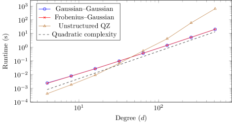
Figure 3: Test of the quadratic complexity in the degree $d$ of the matrix polynomial, $k=4$, and the tests were averaged over $10$ runs. The runtime is compared with the one of the unstructured QZ algorithm from LAPACK. The dashed line represents a quadratic dependence of the runtime on the degree and is added for reference. The runtimes are reported for (Frobenius,Gaussian)-factored and (Gaussian,Gaussian)-factored pencils, whose timings are almost indistinguishable.

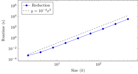
Figure 4: Test of the complexity in the size of the matrices $k$. The examples all have degree $d=4$ and for each combination of $d$ and $k$ $10$ tests were run.

10.2 Backward stability of the Schur form

In Section 9 we provided bounds on the backward error of the computed Schur form. In order to validate these bounds we have measured the backward error on the computed upper triangular pencil $\hat{S}-\lambda\hat{T}$ by evaluating $\lVert U\hat{S}V^{*}-S\rVert_{F}$ and $\lVert U\hat{T}V^{*}-T\rVert_{F}$, where $S-\lambda T$ is the companion pencil associated to a matrix polynomial with random coefficients. We have run 1000 experiments for $k=8$ and $d=10$. The results are reported in Figure 5 for a (Frobenius,Gaussian)-factored pencil and in Figure 6 for a (Gaussian,Gaussian)-factored pencil. We see that, even though both approaches exhibit a quadratic growth in $S$, the (Gaussian,Gaussian)-factorization provides, for this test setting, the best backward error. Both plots also show that the bounds that we have found are asymptotically tight.

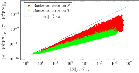
Figure 5: Backward error on the computed Schur form for different values of $\lVert S\rVert_{F}$ and $\lVert T\rVert_{F}$. We took $k=8$, $d=10$ and ran 1000 tests. For $S$ a Frobenius factorization and for $T$ a Gaussian factorization was used. The dashed lines represent a reference line for the quadratic complexity.

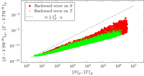
Figure 6: Backward error on the computed Schur form for different values of $\lVert S\rVert_{F}$ and $\lVert T\rVert_{F}$. We took $k=8$, $d=10$ and 1000 runs. In this example the Gaussian factorization has been used for both matrices $S$ and $T$.

10.3 Computing eigenvectors: complexity and stability

Finally, we have computed the eigenvalues and the eigenvectors of random matrix polynomials of degree $d=4$ and size $k=8$. We have generated the coefficients drawing the entries from a normal distribution, and we have randomly scaled each coefficient in order to make them of unbalanced norms. More precisely, each coefficient is of the form $2^{\alpha}M$, where the entries of $M$ are distributed as Gaussians with mean $0$ and variance $1$, and $\alpha$ is drawn from the uniform distribution on $[-15,15]$.

According to Tisseur [26], the absolute backward error on a computed eigenpair $(\lambda,v)$ can be evaluated as

$$err(P,\lambda,v)=\lVert P(\lambda)v\rVert\cdot\left(\sum_{j=0}^{d}|\lambda|^{j}\right)^{-1}.$$ (30)

In Figure 7 we report the maximum of the absolute backward errors on the eigenpairs of $P(\lambda)$ computed with our algorithm; on the $x$ axis we have reported the norm of the coefficients of $P(\lambda)$, computed as the Frobenius norm of $[P_{0},\ldots,P_{d}]$. The linear dependence of the backward error on the norm of the coefficients as predicted by Theorem 17 is clearly visible.

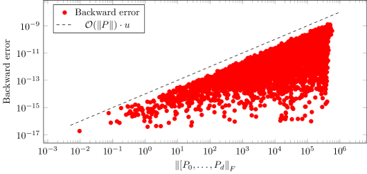
Figure 7: Asolute backward error on the computed eigenpairs of random matrix polynomials $P(\lambda)$ of different norms, according to the formula (30).

     

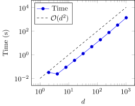
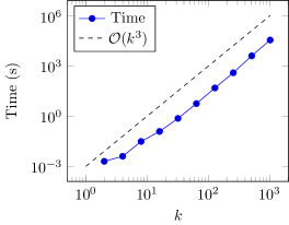
Figure 8: Timings for the computation of all the eigenvectors and eigenvalues of a matrix polynomial as a function of the degree and of the size. The expected quadratic and cubic growth of the complexity are visible.

In Figure 8 we have reported the timings for the computation of all the eigenvectors of al matrix polynomial $P(\lambda)$ for various degrees and sizes. The numerical results show that the behavior remains quadratic in $d$ and cubic in $k$ even when the additional work for the computation of the eigenvectors is required.

10.4 Nonlinear eigenvalue problems: NLEVP

To verify the reliability of our approach we have tested our algorithm on some problems from the NLEVP collection [4]. This archive contains realistic polynomial eigenvalue problems. Most of them do have low degree, however, so we have tested our approach only on problems of degree $4$, namely the orr_sommerfeld, the plasma_drift, and the planar_waveguide problems.

To verify the backward stability, we have reported the backward error on the computed Schur form in Table 1. The pencil was scaled as in Theorem 16.

In Figure 9 we have reported the backward error on the single computed eigenpairs according to (30). The results clearly show that the proposed method performs as well as the classical QZ method.

	$\lVert\delta S\rVert$ (eiscor)	$\lVert\delta S\rVert$ (polyeig)	$\lVert\delta T\rVert$ (eiscor)	$\lVert\delta T\rVert$ (polyeig)
planar_waveguide	8.361 e-14	8.336 e-14	8.910 e-14	7.214 e-14
orr_sommerfeld	3.855 e-14	5.523 e-14	3.285 e-14	4.475 e-14
plasma_drift	6.177 e-14	6.418 e-14	5.705 e-14	4.882 e-14

Table 1: Backward error on the Schur form of the properly scaled companion pencil for some NLEVP problems. The norms reported are the norms of the perturbations to $S$ and $T$.

   

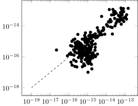
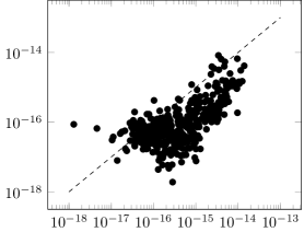
Figure 9: Backward errors on the computed eigenvalues for the orr_sommerfeld (on the left) and plasma_drift (on the right) NLEVP problems. Each point in the plot has the backward error obtained using the QZ algorithm on the (scaled) companion pencil from LAPACK as y coordinate and the algorithm presented in this paper as the x one.

11 Conclusions

A fast, backward stable algorithm was proposed to compute the eigenvalues of matrix polynomials. A factorization of the pencil matrices allowed us to design a product eigenvalue problem operating on a structured factorization of the involved unitary-plus-rank-one factors. Stability was proved and confirmed by the numerical experiments.

References

- [1] J. L. Aurentz, T. Mach, R. Vandebril, and D. S. Watkins, Fast and backward stable computation of roots of polynomials, SIAM Journal on Matrix Analysis and Applications, 36 (2015), pp. 942–973.
- [2] J. L. Aurentz, T. Mach, R. Vandebril, and D. S. Watkins, A note on companion pencils, Contemporary Mathematics, 658 (2016), pp. 91–101.
- [3] P. Benner, V. Mehrmann, and H. Xu, Perturbation analysis for the eigenvalue problem of a formal product of matrices, BIT Numerical Mathematics, 42 (2002), pp. 1–43.
- [4] T. Betcke, N. J. Higham, V. Mehrmann, C. Schröder, and F. Tisseur, NLEVP: a collection of nonlinear eigenvalue problems, ACM Transactions on Mathematical Software, 39 (2013), pp. 7:1–7:28.
- [5] D. Bini and B. Meini, On the solution of a nonlinear matrix equation arising in queueing problems, SIAM Journal on Matrix Analysis and Applications, 17 (1996), pp. 906–926.
- [6] D. A. Bini and V. Noferini, Solving polynomial eigenvalue problems by means of the Ehrlich–Aberth method, Linear Algebra and its Applications, 439 (2013), pp. 1130–1149.
- [7] A. W. Bojanczyk, G. H. Golub, and P. Van Dooren, Periodic Schur decomposition: algorithms and applications, in San Diego’92, International Society for Optics and Photonics, 1992, pp. 31–42.
- [8] T. R. Cameron and N. I. Steckley, On the application of Laguerre’s method to the polynomial eigenvalue problem. Arxiv:1703.08767, 2017.
- [9] S. Delvaux, K. Frederix, and M. Van Barel, An algorithm for computing the eigenvalues of block companion matrices, Numerical Algorithms, 62 (2012), pp. 261–287.
- [10] F. M. Dopico, P. Lawrence, J. Pérez, and P. Van Dooren, Block Kronecker linearizations of matrix polynomials and their backward errors, Tech. Rep. 2016.34, Manchester Institute for Mathematical Sciences, School of Mathematics, The University of Manchester, 2016.
- [11] A. Edelman and H. Murakami, Polynomial roots from companion matrix eigenvalues, Mathematics of Computation, 64 (1995), pp. 763–776.
- [12] C. Effenberger and D. Kressner, Chebyshev interpolation for nonlinear eigenvalue problems, BIT Numerical Mathematics, 52 (2012), pp. 933–951.
- [13] Y. Eidelman, I. C. Gohberg, and I. Haimovici, Separable Type Representations of Matrices and Fast Algorithms – Volume 2: Eigenvalue Method, no. 235 in Operator Theory: Advances and Applications, Springer Basel, 2013.
- [14] J. G. F. Francis, The QR Transformation a unitary analogue to the LR transformation–Part 1, The Computer Journal, 4 (1961), pp. 265–271.
- [15] , The QR Transformation–Part 2, The Computer Journal, 4 (1962), pp. 332–345.
- [16] F. R. Gantmacher, The Theory of Matrices, Vol II, Chelsea, New York, USA, 1974.
- [17] I. Gohberg, P. Lancaster, and L. Rodman, Matrix polynomials, vol. 58, SIAM, Philadelphia, USA, 1982.
- [18] N. J. Higham, Accuracy and Stability of numerical algorithms, SIAM, Philadelphia, USA, 1996.
- [19] N. J. Higham, D. S. Mackey, and F. Tisseur, The conditioning of linearizations of matrix polynomials, SIAM Journal on Matrix Analysis and Applications, 28 (2006), pp. 1005–1028.
- [20] P. Lancaster, Lambda-Matrices and Vibrating Systems, Courier Corporation (Dover Publications), New York, USA, 2002.
- [21] T. Mach and R. Vandebril, On deflations in extended QR algorithms, SIAM Journal on Matrix Analysis and Applications, 35 (2014), pp. 559–579.
- [22] D. S. Mackey, N. Mackey, C. Mehl, and V. Mehrmann, Structured polynomial eigenvalue problems: good vibrations from good linearizations, SIAM Journal on Matrix Analysis and Applications, 28 (2006), pp. 1029–1051.
- [23] , Vector spaces of linearizations for matrix polynomials, SIAM Journal on Matrix Analysis and Applications, 28 (2006), pp. 971–1004.
- [24] C. B. Moler and G. W. Stewart, An algorithm for generalized matrix eigenvalue problems, SIAM Journal on Numerical Analysis, 10 (1973), pp. 241–256.
- [25] L. Robol, Exploiting rank structures for the numerical treatment of matrix polynomials, PhD thesis, University of Pisa, Italy, 2015.
- [26] F. Tisseur, Backward error and condition of polynomial eigenvalue problems, Linear Algebra and its Applications, 309 (2000), pp. 339–361.
- [27] M. Van Barel, Designing rational filter functions for solving eigenvalue problems by contour integration, Linear Algebra and its Applications, 502 (2016), pp. 346–365.
- [28] R. Vandebril, Chasing bulges or rotations? A metamorphosis of the QR-algorithm, SIAM Journal on Matrix Analysis and Applications, 32 (2011), pp. 217–247.
- [29] R. Vandebril and D. S. Watkins, An extension of the QZ algorithm beyond the Hessenberg-upper triangular pencil, Electronic Transactions on Numerical Analysis, 40 (2012), pp. 17–35.
- [30] D. S. Watkins, Product eigenvalue problems, SIAM Review, 47 (2005), pp. 3–40.
- [31] , The Matrix Eigenvalue Problem: GR and Krylov Subspace Methods, SIAM, Philadelphia, USA, 2007.