Improvement of flatness for nonlocal phase transitions

Abstract.

We establish an improvement of flatness result for critical points of Ginzburg-Landau energies with long-range interactions. It applies in particular to solutions of $(-\Delta)^{s/2}u=u-u^{3}$ in $\mathbb{R}^{n}$ with $s\in(0,1)$. As a corollary, we establish that solutions with asymptotically flat level sets are $1$D and prove the analogue of the De Giorgi conjecture (in the setting of minimizers) in dimension $n=3$ for all $s\in(0,1)$ and in dimensions $4\leqslant n\leqslant 8$ for $s\in(0,1)$ sufficiently close to $1$.

The robustness of the proofs, which do not rely on the extension of Caffarelli and Silvestre, allows us to include anisotropic functionals in our analysis.

Our improvement of flatness result holds for all solutions, and not only minimizers. This cannot be achieved in the classical case $-\Delta u=u-u^{3}$ (in view of the solutions bifurcating from catenoids constructed in [24]).

1. Introduction

1.1. Ginzburg-Landau energy with long range interactions

The paper is concerned with critical points of the following Ginzburg-Landau energy with long range interactions

$$J(v):=\frac{1}{4}\iint_{\mathbb{R}^{n}\times\mathbb{R}^{n}}\frac{|v(x)-v(z)|^{2}}{\|x-z\|_{K}^{n+s}}\,dx\,dz+\int_{\mathbb{R}^{n}}W(v)\,dx.$$

Here, $K$ is an even and $C^{1,1}$ convex body, $\|\cdot\|_{K}$ denotes the norm of $\mathbb{R}^{n}$ with unit ball $K$, and $W$ is a double-well potential.

Such energies naturally arise in several contexts, such as phase transitions, atom dislocations in crystals, mathematical biology, etc. (see e.g. Section 2 in [26], the Appendix in [21], the Introduction in [13], and also [8] and the references therein for a series of motivations under different perspectives).

We establish a improvement of flatness result for the level sets of critical points $J$. That is, for solutions $u$ of

$$Lu=f(u)\quad\mbox{in }\mathbb{R}^{n},$$ (1.1)

where $L$ is an elliptic scaling invariant operator of order $s\in(0,1)$, of the form

$$Lu(x):=\int_{\mathbb{R}^{n}}\frac{u(x)-u(x+y)}{\|y\|_{K}^{n+s}}\,dy.$$ (1.2)

Throughout the paper $f=-W^{\prime}$ will be the derivative of the double-well potential. Note that the case of the fractional Laplacian $L=(-\Delta)^{s/2}$ corresponds to $K$ being a ball —and thus $\|\cdot\|_{K}=|\,\cdot\,|$.

1.2. Large scale behavior and De Giorgi conjecture

If $v$ is a minimizer of $J$ in $\mathbb{R}^{n}$ (locally) then $v_{\varepsilon}(x)=v(x/\varepsilon)$ is a minimizer of

$$J_{\varepsilon}(v):=\frac{1}{4}\iint_{\mathbb{R}^{n}\times\mathbb{R}^{n}}\frac{|v(x)-v(z)|^{2}}{\|x-z\|_{K}^{n+s}}\,dx\,dz+\varepsilon^{-s}\int_{\mathbb{R}^{n}}W(v)\,dx$$

and solves the equation

$$Lv_{\varepsilon}=\varepsilon^{-s}f(v_{\varepsilon}).$$

By the methods introduced in [19] for the analysis of nonlocal phase transitions, one can prove that $\|\nabla v_{\varepsilon}\|_{L^{1}(B_{R})}\leqslant CR^{n-1}$ for all $R\geqslant 1$, with $C$ depending only on $n,s,K$. In particular, one can show that (up to subsequence)

$$v_{\varepsilon}\rightarrow\chi_{E}-\chi_{E^{c}}\quad\mbox{ in }L^{1}_{\rm loc}(\mathbb{R}^{n})$$ (1.3)

where $E$ is a minimizer of a fractional perimeter. More precisely, when $K$ is a ball one obtains the isotropic fractional perimeter (Caffarelli, Roquejoffre, and Savin [14]) while for other $K$ one obtains the anisotropic fractional perimeters (Ludwig in [34]).

In the range $s\in[1,2]$, in the isotropic setting one still has (1.3) but then $E$ is known to be a minimizer of the classical perimeter. This was proven in [35, 41] through $\Gamma-$convergence results.

We thus see that there is a striking difference between the two regimes $s\in(0,1)$ and $s\in[1,2]$ as far as asymptotic behavior at large scales is concernd. We use the wording genuinely nonlocal regime to refer to the case $s\in(0,1)$ because the long-range interactions survive in the asymptotic limit.

For $s=2$, the link between minimizers of the Ginzburg-Landau energy and minimizers of the classical perimeter motivates a famous conjecture of Ennio De Giorgi  [22]. This conjecture states that “every bounded solution of $-\Delta u=u-u^{3}$ in $\mathbb{R}^{n}$ that is monotone in one variable, say $\partial_{x_{n}}u>0$, is $1$D in dimension $n\leqslant 8$. Namely, its level sets are parallel hyperplanes”.

The threshold $n=8$ is related the classical results on entire minimal graphs: affine functions (hyperplanes) are the only entire minimal graphs up to dimension $n=8$ (see [45]) while non-affine examples can be found in dimensions $n=9$ or higher (see [7]).

Positive answers to De Giorgi conjecture have been established for $n=2$ in [33], $n=3$ in [3, 2] and, in the setting of minimizers, for $4\leqslant n\leqslant 8$ in [37]. A non- $1$D example was constructed in [23] for $n=9$. See also the excellent survey [38] for the history of the conjecture and the known results.

To prove the conjecture (in the setting of minimizers) for $4\leqslant n\leqslant 8$, Savin established in the celebrated paper [37] that

$$\left.\begin{array}[]{c}\mbox{ $u$ is a minimizing solution of $-\Delta u=u-u^{3}$,}\\ \mbox{and the level sets of $u$ are asymptotically flat}\end{array}\right\}\quad\Rightarrow\quad\mbox{$u$ is $1$D. }$$ (1.4)

Here, the word “minimizing” refers to the associated energy

$$\int_{\mathbb{R}^{n}}\frac{1}{2}|\nabla u|+\frac{1}{4}(1-u^{2})^{2}\,dx$$

while “the level sets of $u$ are asymptotically flat” means that $\{u_{\varepsilon}=\theta\}$ converges uniformly on compact sets to a hyperplane for all $\theta\in(-1,1)$ as $\varepsilon\downarrow 0$.

Since, as explained above, for $s\in[1,2]$ the Ginzburg-Landau energy behaves asymptotically like the classical perimeter, it is natural to conjecture that the statement of De Giorgi holds also true for $(-\Delta)^{s/2}u=u-u^{3}$ whenever $s\in[1,2]$.

In this direction the cases $s\in[1,2]$ are currently as well understood as the case $s=2$ —only the construction of a counterexample for $n=9$ is missing to have a full parallelism of results. These results have been obtain in  [12, 46, 9, 10, 44, 40]. In particular, the analogue of (1.4) for $s\in(1,2)$ has been recently established by Savin in [40] where also the important case of the half Laplacian $s=1$ has been announced.

For $s\in(0,1)$ it is natural to expect a analogue of the De Giorgi conjecture in sufficiently low dimensions. The heuristic giving $n=8$ as a critical dimension is only valid in the case $s\in[1,2]$ and the $1$D symmetry up to dimension $n=8$ is not expected for all $s\in(0,1)$ but just for $s$ sufficiently close to $1$. Despite of several works in that direction, up to now a positive result to the conjecture for $s\in(0,1)$ was only known in dimension $n=2$ —as established in [46, 11].

In this paper we prove —see the forthcoming Theorem 1.2—

$$\left.\begin{array}[]{c}\mbox{ $u$ is a solution of $Lu=u-u^{3}$ with $s\in(0,1)$,}\\ \mbox{and the level sets of $u$ are asymptotically flat}\end{array}\right\}\quad\Rightarrow\quad\mbox{$u$ is $1$D. }$$ (1.5)

As a consequence, we establish the De Giorgi conjecture (in the minimizer setting) in the following cases

• in dimension $n=3$, for all $s\in(0,1)$

• in dimension $4\leqslant n\leqslant 8$ for $s\in(0,1)$ sufficiently close to $1$.

Let us stress a fundamental difference between the classical case in (1.4) —or similarly the cases $s\in[1,2)$— and the nonlocal case in (1.5). Namely, the results for $s\in[1,2]$ are for minimizers while our result for $s\in(0,1)$ holds in the more general setting of solution (critical points). This is a feature of the genuinely nonlocal regime $s\in(0,1)$ that is not expected to be true in the case $s\in[1,2]$ (in view of the solutions bifurcating from catenoids constructed in [24] for $s=2$).

In the cases $s\in[1,2]$, the implication (1.4) follows as a direct consequence of an important improvement of flatness result for level sets of solutions to $(-\Delta)^{s/2}u=u-u^{3}$. This result is in the same spirit of the one of De Giorgi for classical minimal surfaces. Similarly, for $s\in(0,1)$ the implication (1.5) follows from an improvement of flatness result for solutions of $Lu=f(u)$, stated next in Subsection 1.4. As we will see, however, in the case $s\in(0,1)$ the improvement of flatness does not yield as a direct consequence (1.5) as for $s\in[1,2]$.

Before stating our main results let us make quantitative versions of our assumptions.

1.3. Quantitative assumptions on $L$ and $f$

We assume that the convex set $K$ defining the operator $L$ satisfies

$$K\subset B_{1} \partial K r_{K}>0 K$$ and each point of can be touched by a ball of radius contained in . (H1)

This is a quantitative version of $K$ being $C^{1,1}$.

We assume that $f$ belongs to $C^{1}\big{(}[-1,1]\big{)}$ and satisfies, for some $\kappa>0$ and $c_{\kappa}>0$,

$$f(-1)=f(1)=0\quad\mbox{and}\quad f^{\prime}(t)<-c_{\kappa}\quad\mbox{for }t\in[-1,-1+\kappa]\cup[1-\kappa,1].$$ (H2)

Moreover, we assume that

$$\mbox{there exists $\phi_{0}$ satisfying}\quad\begin{cases}\mathcal{L}\phi_{0}=f(\phi_{0})\ &\mbox{in }\mathbb{R},\\ \phi_{0}^{\prime}>0&\mbox{in }\mathbb{R},\\ \phi_{0}(0)=0,\\ \displaystyle\lim_{x\to\pm\infty}\phi_{0}=\pm 1,\end{cases}$$ (H3)

where $\mathcal{L}$ denotes (here and throughout the paper) the fractional Laplacian in dimension one (without normalization constant)— see (2.6).

We remark that assumption (H2) and (H3) are satisfied when $f=-W^{\prime}$, with $W$ being a $C^{2}$ double-well potential with wells (i.e. minima) at $\pm 1$ and satisfying that $W^{\prime\prime}>0$ near $\pm 1$. Indeed, the existence a one-dimensional heteroclinic solution is proven in [36, 11] (see also [20] for the case of general kernels) and thus (H3) is satisfied.

The constants in the estimates will also depend on

$$l_{\kappa}:=\inf\big{\{}\,l>0\ :\ \phi_{0}\big{(}[-l,l]\big{)}.\supset[-1+\kappa,1-\kappa]\big{\}}.$$ (1.6)

Note that $l_{\kappa}$ is (half of) the length of the symmetric interval where the transition of $\phi_{0}$ essentially occurs.

1.4. Improvement of flatness result

In the framework that we have just introduced, we are now in the position of stating our main result as follows.

Throughout the paper, we call a constant universal if it depends only on $n$, $s$, $r_{K}$ , $\kappa$, $c_{\kappa}$ and $l_{\kappa}$, see Subsections 2.2 and 1.3. In particular, universal constants depend only on $n$, $L$, and $f$.

In the statement of the next theorem, for fixed $\alpha_{0}>0$, given $a\in(0,1)$ we define

$$j_{a}:=\left\lfloor\frac{\log a}{\log(2^{-\alpha_{0}})}\right\rfloor.$$ (1.7)

Note that $j_{a}$ is a nonnegative integer and that $2^{\alpha_{0}j_{a}}$ is comparable to $1/a$.

Theorem 1.1.

Let $s\in(0,1)$. Assume that $L$ satisfies $\eqref{assumpK}$ and that $f$ satisfies (H2) and (H3). Then there exist universal constants $\alpha_{0}\in(0,s/2)$, $p_{0}\in(2,\infty)$ and $a_{0}\in(0,1/4)$ such that the following statement holds.

Let $a\in(0,a_{0}]$ and $\varepsilon\in(0,a^{p_{0}}]$. Let $u:\mathbb{R}^{n}\rightarrow(-1,1)$ be a solution of $Lu=\varepsilon^{-s}f(u)$ in $B_{2^{j_{a}}}$ such that $0\in\{-1+\kappa\leqslant u\leqslant 1-\kappa\}$ and

$$\{\omega_{j}\cdot x\leqslant-a2^{j(1+\alpha_{0})}\}\,\subset\,\{u\leqslant-1+\kappa\}\,\subset\,\{u\leqslant 1-\kappa\}\,\subset\,\{\omega_{j}\cdot x\leqslant a2^{j(1+\alpha_{0})}\}\quad\mbox{in }B_{2^{j}},$$

for $0\leqslant j\leqslant j_{a}$, where $\omega_{j}\in S^{n-1}$.

Then,

$$\left\{\omega\cdot x\leqslant-\frac{a}{2^{1+\alpha_{0}}}\right\}\,\subset\,\{u\leqslant-1+\kappa\}\,\subset\,\{u\leqslant 1-\kappa\}\,\subset\,\left\{\omega\cdot x\leqslant\frac{a}{2^{1+\alpha_{0}}}\right\}\quad\mbox{in }B_{1/2},$$

for some $\omega\in S^{n-1}$.

In order to explain more intuitively of Theorem 1.1, let us introduce some (informal) terminology. We call transition level sets (of $u$) all the level sets $\{u=\theta\}$ for $\theta\in(-1+\kappa,1-\kappa)$. We say that the transition level sets are flat at a scale $R$ if they are trapped, after some rotation, in a cylinder $B^{\prime}_{R}\times(-aR,aR)$. We call flatness the adimensional quantity $a$.

With this terminology, Theorem 1.1 says that if the transition level sets are flat enough at a very large scale, then its flatness improves geometrically at smaller scales. However, as we will see in more detail in Section 7, the geometric improvement of the flatness does not hold up to scale 1 but only up to some (still very large) mesoscale. This is because we need to assume $\varepsilon\leqslant a^{p_{0}}$ with $p_{0}$ large and not just $\varepsilon\leqslant ca$. This is related to the fact that the $1$D solution $\phi_{0}$ from (H3) decays to $\pm 1$ when $x\to\pm\infty$ only at a slow algebraic rate comparable to $|x|^{-s}$. We will comment more on this important difference with respect to [37] later on.

Theorem 1.1 can be also understood as an approximate $C^{1,\alpha}$ regularity result for level sets. Namely, if the transition level sets of the solution of $Lu=\varepsilon^{-s}f(u)$ in $B_{1}$ are trapped between two parallel planes close enough to the origin, and $\varepsilon$ is small enough, then the transition occurs essentially on a $C^{1,\alpha}$ graph in $B_{1/2}$ up to errors that decay algebraically (in $\varepsilon$) as $\varepsilon\downarrow 0$. The limit case as $\varepsilon\downarrow 0$ of this result plays a crucial role in the regularity theory of nonlocal minimal surfaces; see Theorem 6.8 in [14].

An analogue of Theorem 1.1 for $s\in(1,2)$ has been obtained very recently by Savin in [40, Theorem 6.1] by using a robust version [39] of the original proof in [37]. The important case of the half Laplacian ($s=1$) turns out to be a borderline case for the method in [39, 40], and a similar improvement of flatness result for $s=1$ has been announced also in [40]. Despite of the analogy in the statements, there exist fundamental difference between Theorem 1.1 and Theorem 6.1 of [40]. Indeed,

1. Theorem 1.1 is for solutions (not necessarily minimizers)

2. $\varepsilon\leqslant a^{p_{0}}$ is assumed Theorem 1.1 which is stronger than $\varepsilon\leqslant ca$ in [40] (the result for $s\in(0,1)$ is probably not true under the assumption $\varepsilon\leqslant ca$ due to the very slow decay of $u$ to $\pm 1$)

3. Theorem 1.1 includes anisotropic functionals (in particular our proofs do not make us of the Caffarelli Silvestre extension).

1.5. $1$D symmetry of asymptotically flat solutions

An important application Theorem 1.1 is the following rigidity result for solutions in the whole space with asymptotically flat level sets.

We say that a function $u:\mathbb{R}^{n}\to\mathbb{R}$ is $1$D if there exist $\bar{u}:\mathbb{R}\to\mathbb{R}$ and $\bar{\omega}\in S^{n-1}$ such that $u(x)=\bar{u}(\bar{\omega}\cdot x)$ for any $x\in\mathbb{R}^{n}$.

Theorem 1.2 (One-dimensional symmetry for asymptotically flat solutions).

Let $s\in(0,1)$. Assume that $L$ satisfies $\eqref{assumpK}$ and that $f$ satisfies (H2) and (H3) and let $u$ be a solution of $Lu=f(u)$ in $\mathbb{R}^{n}$.

Assume that there exist $R_{0}\geqslant 1$ and $a:(R_{0},+\infty)\rightarrow(0,1]$ such that $a(R)\downarrow 0$ as $R\uparrow+\infty$ and such that, for all $R>R_{0}$, we have

$$\{\omega\cdot x\leqslant-a(R)R\}\subset\{u\leqslant-1+\kappa\}\subset\{u\leqslant 1-\kappa\}\subset\{\omega\cdot x\leqslant a(R)R\}\quad\mbox{in }B_{R},$$ (1.8)

for some $\omega\in S^{n-1}$, which may depend on $R$.

Then, $u$ is $1$D.

A similar result for $s\in(1,2)$ is given in [40, Theorem 1.1]. In [40], this asymptotic result is a direct application of the improvement of flatness result [40, Theorem 6.1] and rescaling. In our case, Theorem 1.2 will still be a consequence of Theorem 1.1, but not an immediate one. Indeed:

• In [37, 40] the improvement of flatness only requires $\varepsilon\leqslant ca$, and can be iterated from a large scale $R$ all the way up to scale $1$ (thus giving the rigidity when letting $R\to\infty$).

• In contrast, Theorem 1.1 requires $\varepsilon\leqslant a^{p_{0}}$ and thus we can only improve the flatness geometrically from a large ball $B_{R}$ up to a still large mesoscopic ball $B_{r}$ with $r=R^{1-\delta}$.

Due to this, the proof of Theorem 1.2 becomes more interesting, and requires a suitable multiscale iteration of Theorem 1.1, combined with the use of the sliding method of Berestycki, Caffarelli and Nirenberg [5, 6] in its full strength. See Subsection 1.7 for further details on the proofs.

1.6. Application to the De Giorgi conjecture for $s\in(0,1)$

Let us now consider the concrete case of minimizing solutions of the nonlocal Allen-Cahn equation $(-\Delta)^{s/2}u=u-u^{3}$, with $s\in(0,1)$. We remark that the problem is variational, with associate energy functional given by

$${\mathcal{E}}(u,\Omega):={\mathcal{E}^{\rm Dir}}(u,\Omega)+\int_{\Omega}(1-u^{2}(x))^{2}\,dx,$$ (1.9)

where, for some appropriate constant $C_{n,s}>0$,

$${\mathcal{E}^{\rm Dir}}(u,\Omega):=C_{n,s}\iint_{\mathbb{R}^{2n}\setminus(\mathbb{R}^{n}\setminus\Omega)^{2}}\frac{|u(x)-u(y)|^{2}}{|x-y|^{n+s}}\,dx\,dy.$$ (1.10)

We say that a solution $u$ of $(-\Delta)^{s/2}u=u-u^{3}$ is a minimizer of $\mathcal{E}$ in $\mathbb{R}^{n}$ if

$${\mathcal{E}}(u,B)\leqslant{\mathcal{E}}(u+\varphi,B),$$

for any ball $B\subset\mathbb{R}^{n}$ and any $\varphi\in C^{\infty}_{0}(B)$ (notice that, for simplicity, we are dropping the normalization constant in the fractional Laplace framework).

In this setting, we have:

Theorem 1.3 (One-dimensional symmetry in the plane).

Let $u$ be a minimizer of $\mathcal{E}$ in $\mathbb{R}^{2}$.

Then, $u$ is $1$D.

Theorem 1.3 has been also proved, by different methods, in [11, 46]. On the other hand, the following results are, as far as we know, completely new, since they deal with higher-dimensional spaces (indeed, the only symmetry results known for the fractional Allen-Cahn equation are the ones in [9, 10], which hold in dimension $n=3$ with $s\in[1,2)$, while we will consider now the case $n\geqslant 3$ and $s\in(0,1)$, under different assumptions).

Theorem 1.4 (One-dimensional symmetry for monotone solutions in $\mathbb{R}^{3}$).

Let $n\leqslant 3$ and $u$ be a solution of $(-\Delta)^{s/2}u=u-u^{3}$ in $\mathbb{R}^{n}$.

Suppose that

$$\frac{\partial u}{\partial x_{n}}(x)>0\quad{\mbox{ for any }}x\in\mathbb{R}^{n}$$

and

$$\lim_{x_{n}\to\pm\infty}u(x^{\prime},x_{n})=\pm 1.$$

Then, $u$ is $1$D.

Theorem 1.4 has also been recently exploited in [25] in order to obtain additional results of De Giorgi type.

The next two results deal with the case in which the fractional parameter $s$ is sufficiently close to $1$ (that is, roughly speaking, when the nonlocal diffusive operator is sufficiently close to $\sqrt{-\Delta}$). In this case, it is known that the minimizers of the corresponding geometric problem of fractional perimeters are close to the classical minimal surfaces (see [18]). This fact provides an additional rigidity of the interfaces that we can exploit in order to obtain symmetry results.

Theorem 1.5 (One-dimensional symmetry when $s$ is close to 1).

Let $n\leqslant 7$. Then, there exists $\eta_{n}\in(0,1)$ such that for any $s\in[1-\eta_{n},\,1)$ the following statement holds true.

Let $u$ be a minimizer of $\mathcal{E}$ in $\mathbb{R}^{n}$. Then, $u$ is $1$D.

Theorem 1.6 (One-dimensional symmetry for monotone solutions in $\mathbb{R}^{8}$ when $s$ is close to $1$).

Let $n\leqslant 8$. Then, there exists $\eta_{n}\in(0,1)$ such that for any $s\in[1-\eta_{n},\,1)$ the following statement holds true.

Let $u$ be a solution of $(-\Delta)^{s/2}u=u-u^{3}$ in $\mathbb{R}^{n}$.

Suppose that

$$\frac{\partial u}{\partial x_{n}}(x)>0\quad{\mbox{ for any }}x\in\mathbb{R}^{n}$$ (1.11)

and

$$\lim_{x_{n}\to\pm\infty}u(x^{\prime},x_{n})=\pm 1.$$ (1.12)

Then, $u$ is $1$D.

1.7. Overview of the proofs and organization of the paper

The proof of Theorem 1.1 follows the classical “improvement of flatness strategy” that was pioneered by Savin in [37] for the case of level sets of classical phase transitions. The same general approach was suitably modified in [14] in the context of nonlocal minimal surfaces. Let us give next the “big picture” of it in order to explain the structure of the paper —we will assume here for simplicity $L=(-\Delta)^{s/2}$.

Very roughly, we take a sequence $u_{a}$ of solutions of $(-\Delta)^{s/2}u_{a}=\varepsilon^{-s}f(u_{a})$ such that the transition level sets of $u_{a}$ are trapped in a very flat cylinder $\{|x^{\prime}|\leqslant 1,|x_{n}|\leqslant a\}$. We assume that $\varepsilon<{a^{p_{0}}}$ for $p_{0}$ large and we show that $u_{a}\approx\pm 1$ outside of essentially a $n-1$ dimensional surface (that is very flat but possibly very irregular). We then consider “vertical rescalings”

$$(x^{\prime},x_{n})\mapsto\left(x^{\prime},\frac{x_{n}}{a}\right)$$

of these “transition surfaces”.

A main step in the proof then consists in proving that the vertical rescalings of the “transition surfaces” are compact as $a\downarrow 0$ and converge to a continuous graph $g:\mathbb{R}^{n-1}\rightarrow\mathbb{R}$.. To achieve this compactness we need a “Hölder type” estimate, or improvement of oscillation, for vertical rescalings of level sets. The proof of this improvement of oscillation estimate is given in Section 4. It requires to build fine barriers for the semilinear equation and several auxiliary result that are given in Section 2 and 3.

A second step in the proof is to show that the limit graph $g$ is a viscosity solution of the linear translation invariant elliptic equation $(-\Delta)^{\frac{1+s}{2}}g=0$ in $\mathbb{R}^{n-1}$. This is done in Section 5.

Finally we obtain the improvement by compactness, inheriting it from the $C^{1,\alpha}$ regularity of $(-\Delta)^{\frac{1+s}{2}}g=0$. This is done in Section 6.

The rest of the paper, namely Sections 7 and 8, is devoted to the proof of Theorem 1.2 and its consequences. As explained before, Theorem 1.2 follows from Theorem 1.1 but not in a straightforward way. Let us summarize next the main steps of its proof.

We use two different iterations of Theorem 1.1. The first iteration, that we informally call “preservation of flatness”, is given in Corollary 7.1. The second iteration, really a geometric “improvement of flatness”, is given in Corollary 7.2. Corollary 7.2 is stronger in the sense that the flatness is improved geometrically in a sequence of dyadic balls, but only up to a large mesoscale. In Corollary 7.1 the flatness does not improve but is just preserved across scales but, as a counterpart, it gives information up to scale 1.

To prove Theorem 1.2 we need to combine Corollary 7.1 with a multi-scale application of Corollary 7.2. Doing so, we prove that the transition level sets are trapped, in all of $\mathbb{R}^{n}$, between a Lipschitz graph and a finite vertical translation of it. Then, we need to use the sliding method (in its full strength) to conclude that the level sets of the solution are indeed flat.

Notation

For the convenience of the reader we gather here the notation that we will follow throughout all the paper. The following list of notations is just for quick reference and all the notations are introduced (again) within the text at their first appearance.

• $L$, $f$ are the nonlocal elliptic operator and the nonlinearity, respectively, see (1.1).

• $n\geqslant 2$, $s\in(0,1)$, $K$ are, respectively, the dimension, the order of the operator, and the even, $C^{1,1}$ convex set defining the norm $\|\cdot\|_{K}$ in the definition of $L$.

• ${\mathcal{L}}$ denotes the one-dimensional fractional Laplacian as in (2.6).

• $r_{K}$ is the inner curvature radius of $\partial K$; see (H1).

• $\kappa$, $c_{\kappa}$ and $l_{\kappa}$ are the constants in the quantitative assumptions of $f$, see Subsection 1.4.

• We will call a constant universal if it depends only on $n$, $s$, $r_{K}$ , $\kappa$, $c_{\kappa}$ and $l_{\kappa}$. In particular, universal constants depend only on $n$, $L$, and $f$.

• $\lambda,\Lambda$ are the ellipticity constants of $L$, $\mathcal{C}=\mathcal{C}_{L}$ is the convex body with support function $h_{L}$, and $\rho^{\prime}>\rho>0$ are the two constants in its curvature bounds, see Subsection 1.3.

• We write

  $$X\subset Y\quad\mbox{in }B\qquad\mbox{if}\qquad X\cap B\,\subset\,Y\cap B.$$

• We denote by $\|\,\cdot\,\|_{\mathcal{C}}$ the norm with unit ball $\mathcal{C}$. We also denote by $\mathcal{C}_{r}(y)$ the ball of radius $r$ and center $y$ with respect to this norm, namely

  $$\mathcal{C}_{r}(y):=y+r\mathcal{C}.$$

  Notice that when $L$ is the fractional Laplacian $\mathcal{C}_{r}(y)$ is simply $B_{r}(y)$.

• Points in $\mathbb{R}^{n-1}$ will be denoted by $x^{\prime}$ and $x=(x^{\prime},x_{n})$ denotes a point in $\mathbb{R}^{n}$ with $n$-th coordinate $x_{n}$. From now on, we also denote by $B_{r}^{\prime}$ the $(n-1)$-dimensional ball of radius $r>0$.

• $\xi$ denotes the function $\xi:\mathbb{R}^{n-1}\rightarrow\mathbb{R}$ which is defined by

  $$\xi(x^{\prime})=\xi(|x^{\prime}|):=\bigl{(}1+|x^{\prime}|^{2}\bigr{)}^{\frac{1+\alpha}{2}}-1.$$ (1.13)

• Given $b>0$, we denote by $d_{b}$ the signed distance function to the set $\{x_{n}\geqslant b\,\xi(x^{\prime})\}$ with respect to the norm $\|\,\cdot\,\|_{\mathcal{C}}$, that is,

  $$d_{b}(x)=\begin{cases}+\inf\big{\{}\|z-x\|_{\mathcal{C}}\ :\ z_{n}=b\,\xi(z^{\prime})\big{\}},\quad&\mbox{for }x_{n}\geqslant b\,\xi(x^{\prime}),\\ -\inf\big{\{}\|z-x\|_{\mathcal{C}}\ :\ z_{n}=b\,\xi(z^{\prime})\big{\}},&\mbox{for }x_{n}\leqslant b\,\xi(x^{\prime}).\end{cases}$$

• Given $\phi:\mathbb{R}\rightarrow(-1,1)$, for any $x\in\mathbb{R}$, we set

  $$\phi^{b}(x):=\phi\bigl{(}d_{b}(x)\bigr{)}.$$

  Notice that $\phi^{b}:\mathbb{R}\rightarrow(-1,1)$, and it may be seen as a “rearrangement” of the layer solution $\phi$ with respect to the signed distance function.

In addition to the previous notations we use also the following very standard ones.

• Given $r\in\mathbb{R}$, we denote by $r_{+}:=\max\{r,0\}$ and $r_{-}:=\max\{-r,0\}$.

• Given a measurable function $f:X_{1}\times\dots\times X_{m}\to\mathbb{R}$, we use the repeated integral notation

  $$\int_{X_{1}}\,dx_{1}\,\dots\,\int_{X_{m}}\,dx_{m}\,f(x_{1},\dots,x_{m}):=\int_{X_{1}}\left[\dots\int_{X_{m}}f(x_{1},\dots,x_{m})\,dx_{m}\dots\right]\,dx_{1}.$$

2. Approximate solutions via deformation of level sets

In this section we construct approximate solutions in $B_{1}$ by deforming (slightly curving) the flat level sets of a one-dimensional solution.

2.1. A layer cake formula

The main results of this paper are valid for an operator $L$ of the form

$$Lu(x):=\int_{\mathbb{R}^{n}}\big{(}u(x)-u(x+y)\big{)}\frac{\mu\big{(}y/|y|\big{)}}{|y|^{n+s}}\,dy.$$ (2.1)

The measure $\mu$ in (2.1) is often called in jargon the “spectral measure”. By assumption —see (H1) on page H1— we have that $\mu$ satisfies

$$\mu(z)=\mu(-z)\quad\mbox{and}\quad 0<\lambda\leqslant\mu(z)\leqslant\Lambda<+\infty\quad\mbox{for all }z\in S^{n-1}.$$ (2.2)

where $\lambda$, $\Lambda$ are positive constants depending only on $n$, $s$ and $r_{K}$ and are called the ellipticity constants.

Now we give a simple layer cake representation for the integro-differential operators.

We use the notation

$$\chi_{[a_{1},a_{2}]}(\theta):=\left\{\begin{matrix}1&{\mbox{ if }}a_{1}\leqslant a_{2}{\mbox{ and }}\theta\in[a_{1},a_{2}],\\ \,\\ 0&\begin{matrix}{\mbox{ if either }}a_{1}>a_{2},\\ {\mbox{ or }}a_{1}\leqslant a_{2}{\mbox{ and }}\theta\not\in[a_{1},a_{2}].\end{matrix}\end{matrix}\right.$$ (2.3)

Using this, we have the following simple layer cake type representation for nonlocal operators:

Lemma 2.1.

It holds that

$$Lv(x)=\int_{\mathbb{R}^{n}}\,dy\,\int_{\mathbb{R}}\,d\theta\Big{(}\chi_{[v(x+y),v(x)]}(\theta)-\chi_{[v(x),v(x+y)]}(\theta)\Big{)}\,\frac{\mu(y/|y|)}{|y|^{n+s}}.$$ (2.4)

Furthermore, if $x\in\mathbb{R}^{n}$ is such that $v(x)=w(x)$, then

$$Lv(x)-Lw(x)=\int_{\mathbb{R}^{n}}\,dy\,\int_{\mathbb{R}}\,d\theta\Big{(}\chi_{[v(x+y),w(x+y)]}(\theta)-\chi_{[w(x+y),v(x+y)]}(\theta)\Big{)}\,\frac{\mu(y/|y|)}{|y|^{n+s}}.$$ (2.5)

Proof.

By (2.3),

$$(a_{1}-a_{2})_{-}=(a_{2}-a_{1})_{+}=\int_{\mathbb{R}}\chi_{[a_{1},a_{2}]}(\theta)\,d\theta$$

and therefore

$$v(x)-v(x+y) = \big{(}v(x)-v(x+y)\big{)}_{+}-\big{(}v(x)-v(x+y)\big{)}_{-}$$

$$= \int_{\mathbb{R}}\chi_{[v(x+y),v(x)]}(\theta)\,d\theta-\int_{\mathbb{R}}\chi_{[v(x),v(x+y)]}(\theta)\,d\theta.$$

So, we integrate and we find (2.4).

Similarly, we write

$$w(x+y)-v(x+y)=\int_{\mathbb{R}}\chi_{[v(x+y),w(x+y)]}(\theta)\,d\theta-\int_{\mathbb{R}}\chi_{[w(x+y),v(x+y)]}(\theta)\,d\theta,$$

which gives (2.5) after integration. ∎

2.2. The operator $L$ and the convex set $\mathcal{C}_{L}$

Throughout the paper the fractional Laplacian in dimension $1$ (without normalization constant) will be denoted $\mathcal{L}$. Namely, given a bounded $\psi\in C^{2}(\mathbb{R})$, we define

$$\mathcal{L}\psi(z):=\int_{-\infty}^{\infty}\frac{\psi(z)-\psi(z+\zeta)}{|\zeta|^{1+s}}\,d\zeta,\quad z\in\mathbb{R}.$$ (2.6)

For $\psi$ as above, $\omega\in S^{n-1}$ and $h>0$, we define, for any $x\in\mathbb{R}^{n}$,

$$\bar{\psi}_{\omega,h}\,(x):=\psi\left(\omega\cdot\frac{x}{h}\,\right).$$ (2.7)

Then, for each operator $L$ of the form (2.1), let $h_{L}:S^{n-1}\rightarrow(0,\infty)$ be defined as follows. We set $h_{L}(\omega):=h$, where $h>0$ satisfies

$$L\bar{\psi}_{\omega,h}(x)=\mathcal{L}\psi\left(\omega\cdot\frac{x}{h}\right)\ \mbox{for all }\psi\in C^{2}(\mathbb{R})\cap L^{\infty}(\mathbb{R}).$$ (2.8)

Using the function $h_{L}$, we define the closed convex set

$$\mathcal{C}=\mathcal{C}_{L}:=\bigcap_{\omega\in S^{n-1}}\big{\{}x\in\mathbb{R}^{n}\,:\,x\cdot\omega\leqslant h_{L}(\omega)\big{\}}.$$ (2.9)

We notice also that, since $L$ is even, both $h_{L}$ and $\mathcal{C}_{L}$ are even, i.e. symmetric with respect to the origin. In addition, we remark that, when $L=(-\Delta)^{s/2}$, $\mathcal{C}_{L}$ is a ball (centered at $0$).

Our assumption (H1) on $K$ is made in order to guarantee that

$$\partial\,\mathcal{C}_{L} C^{1,1}$$ is and strictly convex. (2.10)

More quantitatively, that there are constants  $\rho^{\prime}>\rho>0$ depending only on $n$, $s$, $K$ such that

the curvatures of $$\partial\,\mathcal{C}_{L} \frac{1}{\rho} \frac{1}{\rho^{\prime}}$$ are bounded above by and below by . (H1’)

We remark that the definition of $h_{L}$ in (2.8) is well posed, and indeed an explicit expression of $h_{L}(\omega)$ is obtained through the formula

$$h_{L}(\omega)=\left(\frac{1}{2}\int_{S^{n-1}}|\omega\cdot\theta|^{s}\,\mu(\theta)\,d\theta\right)^{1/s}.$$ (2.11)

To prove (2.11), we proceed as follows

$$L\bar{\psi}_{\omega,h}\,(x) = \int_{\mathbb{R}^{n}}\left(\psi\left(\omega\cdot\frac{x}{h}\,\right)-\psi\left(\omega\cdot\frac{x+y}{h}\,\right)\right)\,\frac{\mu\big{(}y/|y|\big{)}}{|y|^{n+s}}\,dy$$

$$= \int_{0}^{+\infty}\,d\varrho\,\int_{S^{n-1}}\,d\theta\,\left(\psi\left(\omega\cdot\frac{x}{h}\,\right)-\psi\left(\omega\cdot\frac{x}{h}+\omega\cdot\frac{\varrho\theta}{h}\,\right)\right)\,\frac{\mu(\theta)}{\varrho^{1+s}}$$

$$= \frac{1}{2}\,\int_{-\infty}^{+\infty}\,d\varrho\,\int_{S^{n-1}}\,d\theta\,\left(\psi\left(\omega\cdot\frac{x}{h}\,\right)-\psi\left(\omega\cdot\frac{x}{h}+\omega\cdot\frac{\varrho\theta}{h}\,\right)\right)\,\frac{\mu(\theta)}{|\varrho|^{1+s}}$$

$$= \frac{1}{2}\,\int_{-\infty}^{+\infty}\,d\zeta\,\int_{S^{n-1}}\,d\theta\,\left(\psi\left(\omega\cdot\frac{x}{h}\,\right)-\psi\left(\omega\cdot\frac{x}{h}+\zeta\,\right)\right)\,\frac{|\omega\cdot\theta|^{s}\,\mu(\theta)}{h^{s}\,|\zeta|^{1+s}},$$

where we used the change of variables $\zeta=\frac{\varrho\omega\cdot\theta}{h}$. Hence, if $h=h_{L}(\omega)$ is given by (2.11),

$$L\bar{\psi}_{\omega,h}\,(x)=\int_{-\infty}^{+\infty}\left(\psi\left(\omega\cdot\frac{x}{h}\,\right)-\psi\left(\omega\cdot\frac{x}{h}+\zeta\,\right)\right)\,\frac{d\zeta}{|\zeta|^{1+s}}=\mathcal{L}\psi\left(\omega\cdot\frac{x}{h}\right),$$

that is (2.8).

A special case of (2.11) occurs when the spectral measure is induced by a convex set, namely when

$$\frac{\mu\big{(}y/|y|\big{)}}{|y|^{n+s}}=\frac{1}{\|y\|_{K}^{n+s}}$$

for some convex set $K$, where $\|\cdot\|_{K}$ is the norm with unit ball $K$, that is, for any $p\in\mathbb{R}^{n}$,

$$\|p\|_{K}:=\inf\{t>0{\mbox{ s.t. }}p/t\notin K\}.$$ (2.12)

Then, in this case, an integration in polar coordinates yields

$$h_{L}(\omega)=\left(\frac{1}{2}\,\int_{S^{n-1}}d\theta\frac{|\omega\cdot\theta|^{s}}{\|\theta\|_{K}^{n+s}}\right)^{1/s}=\left(\frac{n+s}{2}\,\int_{S^{n-1}}\,d\theta\int_{0}^{1/\|\theta\|_{K}}\,d\varrho\,|\omega\cdot\theta|^{s}\,\varrho^{n+s-1}\right)^{1/s}$$

$$\qquad\qquad\qquad=\left(\frac{n+s}{2}\,\int_{K}|\omega\cdot x|^{s}dx\right)^{1/s}.$$

As pointed out to us by M. Ludwig, to whom we are indebted for this comment and the interesting references provided, the convex body associated to this support function is the so called “$L_{p}$-intersection body” of $K$. These convex bodies are well studied in convex geometry, in relation to the important Busemann-Petty problem, see [4] and references therein for more information on this subject.

It is proved in [4] that, for any given convex set $K$ (bounded and with nonempty interior) which is symmetric with respect to the origin, the function $h_{L}$ is strictly convex in all the nonradial directions. Also, from (2.11) it follows that $h_{L}$ is $C^{1,1}$ in $\mathbb{R}^{n}\setminus\{0\}$ when $\mu$ is $C^{1,1}$. Actually $\mu\in C^{2-s+\varepsilon}$ suffices since the “kernel” $|\omega\cdot\theta|^{s}$ is $C^{s}$ and this yields a regularity improvement.

When $K$ is any $C^{1,1}$ convex set, the previous observations imply that the set

$$\mathcal{C}^{*}_{L}:=\{h_{L}=1\}$$

is a $C^{1,1}$, even with respect to $0$, strictly convex set. Noting that $\mathcal{C}_{L}$ and $\mathcal{C}^{*}_{L}$ are one the polar body of the other, one can show that $\mathcal{C}_{L}$ is also a $C^{1,1}$, even, strictly convex set. Indeed, since $\mathcal{C}^{*}_{L}$ is a $C^{1,1}$, even, strictly convex set, any point of its boundary can be touched by two even ellipsoids, one contained in, and the other one containing, $\mathcal{C}^{*}_{L}$. Considering the polar transformations of these ellipsoids we show the same property for $\mathcal{C}_{L}$.

The previous discussion can be summarized in the following

Lemma 2.2 ([4]).

If $L$ is of the form (1.2) with $K$ even and satisfying (H1) then $\mathcal{C}_{L}$ satisfies (H1’) for some  $\rho^{\prime}>\rho>0$ depending only on $n$, $s$, $K$.

Remark 2.3.

Theorems 1.1 and 1.2 are valid (and proved here) for general operators of the form (2.1) and under the more general assumption in (H1’) on page H1’ replacing (H1) on page H1.

In view of Remark 2.3, throughout the proofs, the general setting in (2.1) will be assumed, together with (H1’).

2.3. Touching the level sets of the distance function by concentric spheres

This section discuss some geometric features related to the signed anisotropic distance function to a convex set. To this aim, we recall some basic properties of the support function $h_{L}$ defined in (2.11). First of all, for any $x$, $y\in\mathbb{R}^{n}$, the following inequality of Cauchy-Schwarz type holds true

$$x\cdot y\leqslant h_{L}(y)\,\|x\|_{\mathcal{C}}.$$ (2.13)

See e.g. Lemma 1 in [28] for an elementary proof. Note that here $\|\cdot\|_{\mathcal{C}}$ denotes the norm with unit ball $\mathcal{C}=\mathcal{C}_{L}$, that is a convex set different from (although related to) $K$.

As a counterpart of (2.13), we have that equality holds when one of the two vectors is normal to the sphere to which the other vector belongs. More precisely, we have that if $z_{0}\in\mathbb{R}^{n}$, $R>0$, $z\in\partial{\mathcal{C}}_{R}(z_{0})$ and $\omega_{0}\in S^{n-1}$ is the inner normal of $\partial{\mathcal{C}}_{R}(z_{0})$ at the point $z$, then

$$\omega_{0}\cdot(z_{0}-z)=R\,h_{L}(\omega_{0}),$$ (2.14)

see for example Lemma 3 in [28].

Moreover, it is useful to recall that $h_{L}$ is the “support function” of the convex body ${\mathcal{C}}$, namely for any $\omega\in S^{n-1}$ we have that

$$h_{L}(\omega)=\sup_{x\in{\mathcal{C}}}x\cdot\omega,$$ (2.15)

see for instance Lemma 2 in [28].

We recall also here that both $h_{L}$ and $\mathcal{C}$ are even.

Given a nonempty, closed and convex set $K\subset\mathbb{R}^{n}$, we define the anisotropic signed distance function from $K$ as

$$d_{K}(x):=\inf\big{\{}\ell(x)\,:\,\ell(x)=\omega\cdot x+c,\quad h_{L}(\omega)=1,\quad c\in\mathbb{R}\quad\mbox{and}\quad\ell\geqslant 0\ \mbox{ in all of }K\big{\}}.$$ (2.16)

Notice that $d_{K}$ is a concave function, since it is the infimum of affine functions. Moreover, as shown for instance in Proposition 1 of [28], it holds that

$$d_{K}(x)=\begin{cases}+\inf\big{\{}\|z-x\|_{\mathcal{C}}\ :\ z\in\partial K\big{\}}\quad&\mbox{for }x\in K,\\ -\inf\big{\{}\|z-x\|_{\mathcal{C}}\ :\ z\in\partial K\big{\}}&\mbox{for }x\in\mathbb{R}^{n}\setminus K.\end{cases}$$ (2.17)

We have that $d_{K}$ is a Lipschitz function, with Lipschitz constant $1$ with respect to the anisotropic norm, namely, for any $p$, $q\in\mathbb{R}^{n}$,

$$|d_{K}(p)-d_{K}(q)|\leqslant\|p-q\|_{\mathcal{C}},$$ (2.18)

see e.g. Lemma 4 in [28].

With this setting, we can now prove that the level sets of $d_{K}$ are touched by appropriate concentric anisotropic spheres:

Lemma 2.4.

Let $z_{0}\in K=\{d_{K}>0\}$. Assume that $\mathcal{C}_{R}(z_{0})\subset\{d_{K}>0\}$ touches $\partial K=\{d_{K}=0\}$ at some point $\bar{z}\in\{d_{K}=0\}$.

Then, for any $t\in(-\infty,R)$,

$$\begin{split}&{\mbox{the set $\mathcal{C}_{R-t}(z_{0})$ is contained in $\{d_{K}>t\}$}}\\ &{\mbox{and touches $\{d_{K}=t\}$ at the point }}\\ &z:=z_{0}+\frac{R-t}{R}(z-z_{0})\in\big{(}\partial\mathcal{C}_{R-t}(z_{0})\big{)}\cap\{d_{K}=t\}.\end{split}$$ (2.19)

Furthermore, if we denote by $\omega_{0}\in S^{n-1}$ the inner normal of $\partial{\mathcal{C}}_{R}(z_{0})$ at the point $\bar{z}$, it holds that

$$\begin{split}&{\mbox{$R-\|x-z_{0}\|_{\mathcal{C}}\leqslant d_{K}(x)\leqslant$}}\frac{\omega_{0}}{h_{L}(\omega_{0})}\cdot(x-\bar{z}){\mbox{ for any $x\in\mathbb{R}^{n}$,}}\\ &{\mbox{and equalities hold when }}\ x=z_{0}+\frac{R-t}{R}(z-z_{0}),{\mbox{ for some }}t\in(-\infty,R).\end{split}$$ (2.20)

In particular,

$$d_{K}\left(z_{0}+\frac{R-t}{R}(\bar{z}-z_{0})\right)=t.$$ (2.21)

In addition, if $\tau\in(-\infty,R)$ and $z_{\tau}:=z_{0}+\frac{R-\tau}{R}(z-z_{0})$, then

$$\begin{split}&{\mbox{ ${\mathcal{C}}_{|t-\tau|}(z_{\tau})$ is tangent from the outside to the set}}\\ &\left\{x\in\mathbb{R}^{n}{\mbox{ s.t. }}d_{K}(x)\leqslant t\leqslant\frac{\omega_{0}}{h_{L}(\omega_{0})}\cdot(x-z)\right\}\\ &{\mbox{at the point\leavevmode\nobreak\ $z$. }}\end{split}$$ (2.22)

Proof.

The geometric setting of Lemma 2.4 is depicted in Figure 1.

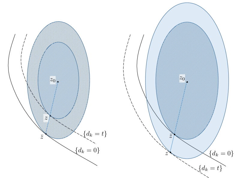
Figure 1. The geometry of Lemma 2.4 when $t\in(0,R)$ and when $t\in(-\infty,0)$.

The proof goes like this. For every $t\in(-\infty,R)$, we have that

$$\|z-z_{0}\|_{\mathcal{C}}=\frac{R-t}{R}\|\bar{z}-z_{0}\|_{\mathcal{C}}=R-t,$$ (2.23)

and therefore

$$z\in\partial\mathcal{C}_{R-t}(z_{0}).$$ (2.24)

In addition, we point out that, for every $t\in(-\infty,R)$,

$$\mathcal{C}_{R-t}(z_{0})\subset\{d_{K}\geqslant t\}.$$ (2.25)

To check this, we distinguish two cases: either $t\geqslant 0$ (i.e. $t\in[0,R)$) or $t<0$. If $t\geqslant 0$, we argue as follows. Let $p\in\mathcal{C}_{R-t}(z_{0})$. Then, for any $q$ with $\|q\|_{\mathcal{C}}\leqslant t$ we have that $p+q\in\mathcal{C}_{R}(z_{0})\subset\{d_{K}\geqslant 0\}$.

Consequently, in light of (2.17), for any affine function $\ell(x)=\omega\cdot x+c$, with $h_{L}(\omega)=1$, $c\in\mathbb{R}$, and such that $\ell\geqslant 0$ in $\{d_{K}>0\}$, it holds that

$$\ell(p+q)\geqslant 0.$$ (2.26)

Therefore, we slide the halfspace with inner normal $\frac{\omega}{|\omega|}$ till it touches $\partial{\mathcal{C}}$ and we take this touching point $q$. Namely, we have $q\in\partial{\mathcal{C}}_{t}$, with $\frac{\omega}{|\omega|}$ as inner normal of $\partial{\mathcal{C}}_{t}$ at $q$. Hence, by (2.14),

$$-\frac{\omega}{|\omega|}\cdot q=t\,h_{L}\left(\frac{\omega}{|\omega|}\right)=\frac{t\,h_{L}(\omega)}{|\omega|}=\frac{t}{|\omega|}.$$

This and (2.26) give that

$$0\leqslant\ell(p+q)=\omega\cdot p+c+\omega\cdot q=\omega\cdot p+c-t.$$

This shows that $\ell(p)\geqslant t$ and so, in view of (2.31), that $d_{K}(p)\geqslant t$, that establishes (2.25) in this case.

So, we now check (2.25) in the case in which $t<0$. For this, let $p\in\mathcal{C}_{R-t}(z_{0})$. If $p\in\mathcal{C}_{R}(z_{0})$, then $d_{K}(p)\geqslant 0\geqslant t$, and we are done, so we can suppose that $p\in\mathcal{C}_{R-t}(z_{0})\setminus\mathcal{C}_{R}(z_{0})$, hence

$$\|p-z_{0}\|_{\mathcal{C}}\in\big{[}R,\,R-t\big{]}.$$

We take

$$q:=z_{0}+\frac{R\,(p-z_{0})}{\|p-z_{0}\|_{\mathcal{C}}}.$$

Notice that $\|q-z_{0}\|_{\mathcal{C}}=R$, hence $q\in\mathcal{C}_{R}(z_{0})\subset\{d_{K}\geqslant 0\}$. This and (2.18) imply that

$$-d_{K}(p)\leqslant d_{K}(q)-d_{K}(p)\leqslant\|q-p\|_{\mathcal{C}}=\big{|}R-\|p-z_{0}\|_{\mathcal{C}}\big{|}=\|p-z_{0}\|_{\mathcal{C}}-R\leqslant(R-t)-R,$$

that gives $d_{K}(p)\geqslant t$, as desired. This completes the proof of (2.25).

Now we check that

$$d_{K}(z)=t.$$ (2.27)

To this aim, we observe that

$$z\in{\mathcal{C}_{R-t}(z_{0})}\subset\{d_{K}\geqslant t\},$$

thanks to (2.24) and (2.25). Consequently, to establish (2.27), we only need to prove that

$$d_{K}(z)\leqslant t.$$ (2.28)

To this goal, if $t\geqslant 0$ we use (2.18) and we see that

$$d_{K}(z)=d_{K}(z)-d_{K}(\bar{z})\leqslant\|z-\bar{z}\|_{\mathcal{C}}=\frac{t}{R}\,\|\bar{z}-z_{0}\|_{\mathcal{C}}\leqslant t,$$

which is (2.27) in this case.

If instead $t<0$, we denote by $\omega_{0}\in S^{n-1}$ the inner normal of $\partial{\mathcal{C}}_{R}(z_{0})$ at the point $z$, and we exploit (2.14) (recall also (2.47)) to see that

$$\begin{split}&d_{K}(z)\leqslant\frac{\omega_{0}}{h_{L}(\omega_{0})}\cdot(z-\bar{z})=\frac{\omega_{0}}{h_{L}(\omega_{0})}\cdot\left(z_{0}-\bar{z}+\frac{R-t}{R}(\bar{z}-z_{0})\right)\\ &\qquad=\frac{t}{R}\frac{\omega_{0}}{h_{L}(\omega_{0})}\cdot(z_{0}-\bar{z})=t.\end{split}$$ (2.29)

This finishes the proof of (2.27).

Then, (2.19) follows from (2.24), (2.25) and (2.27). In turn, (2.19) also implies (2.21).

We also observe that, from the previous considerations, (2.20) follows in a straightforward way using (2.17).

Now we prove (2.22). First of all, we notice that $\|z_{\tau}-\bar{z}\|_{\mathcal{C}}=|t-\tau|$, due to (2.23), so $\bar{z}$ lies on $\partial{\mathcal{C}}_{|t-\tau|}(z_{\tau})$. Thus, to prove the result in (2.22), we need to show that

$$\left\{x\in\mathbb{R}^{n}{\mbox{ s.t. }}\|x-z_{\tau}\|_{\mathcal{C}}<|t-\tau|{\mbox{ and }}d_{K}(x)\leqslant t\leqslant\frac{\omega_{0}}{h_{L}(\omega_{0})}\cdot(x-z)\right\}=\varnothing.$$ (2.30)

Figure 2. Proof of (2.30) when $\tau\geqslant t$ and when $\tau<t$.

For this, we refer to Figure 2, we argue by contradiction and we suppose that there exists $x$ in the set on the left hand side of (2.30). Then, we distinguish two cases, either $\tau\geqslant t$ or $\tau<t$. If $\tau\geqslant t$, we use (2.21) to see that $d_{K}(z_{\tau})=\tau$ and so, exploiting (2.18),

$$0\leqslant t-d_{K}(x)=t-\tau+d_{K}(z_{\tau})-d_{K}(x)\leqslant-|t-\tau|+\|x-z_{\tau}\|_{\mathcal{C}}<0,$$

which is a contradiction. If instead $\tau<t$, using (2.13) and (2.14) we find that

$$t\leqslant\frac{\omega_{0}}{h_{L}(\omega_{0})}\cdot(x-\bar{z})=\frac{\omega_{0}}{h_{L}(\omega_{0})}\cdot(z_{\tau}-\bar{z})+\frac{\omega_{0}}{h_{L}(\omega_{0})}\cdot(x-z_{\tau})$$

$$\qquad\leqslant\tau\frac{\omega_{0}}{h_{L}(\omega_{0})}\cdot\frac{z_{0}-\bar{z}}{R}+\|x-z_{\tau}\|_{\mathcal{C}}=\tau+\|x-z_{\tau}\|_{\mathcal{C}}<\tau+|t-\tau|=t,$$

which is a contradiction. This proves (2.30), which in turn gives (2.22). ∎

2.4. Distance function from a convex graph

Here, we look at the special case of the distance function from a sufficiently flat graph with an appropriate growth. For this, let $\alpha\in(0,s)$ be a fixed constant. Let us introduce the function $\xi:\mathbb{R}^{n-1}\rightarrow\mathbb{R}$ defined by

$$\xi(x^{\prime})=\bigl{(}1+|x^{\prime}|^{2}\bigr{)}^{\frac{1+\alpha}{2}}-1.$$

Note that $\xi(0)=0$ and that $\xi$ is convex with

$$D^{2}\xi={\rm diag}\left(\frac{1+\alpha r^{2}}{1+r^{2}},1,1,\dots,1\right)(1+\alpha)(1+r^{2})^{\frac{\alpha-1}{2}}\geqslant 0$$

in a coordinate system with the first axis pointing in the radial direction.

Given some orthonormal coordinates $x=(x^{\prime},x_{n})$ in $\mathbb{R}^{n}$ and $b>0$, let us define

$$\Gamma_{b}:=\big{\{}\,x_{n}\geqslant b\,\xi(x^{\prime})\,\big{\}}.$$

From the convex set $\Gamma_{b}$ we define the following anisotropic signed distance function

$$d_{b}(x):=\inf\big{\{}\ell(x)\,:\,\ell(x)=\omega\cdot x+c,\quad h_{L}(\omega)=1,\quad c\in\mathbb{R},\ \mbox{and}\quad\ell\geqslant 0\ \mbox{ in all of }\Gamma_{b}\big{\}}.$$ (2.31)

By comparing with (2.16), we have that $d_{b}$ coincides with $d_{K}$ with the particular choice $K:=\Gamma_{b}$. Hence, in view of (2.17), it holds that

$$d_{b}(x)=\begin{cases}+\inf\big{\{}\|x-z\|_{\mathcal{C}}\ :\ z\in\partial\Gamma_{b}\big{\}}\quad&\mbox{for }x\in\Gamma_{b},\\ -\inf\big{\{}\|x-z\|_{\mathcal{C}}\ :\ z\in\partial\Gamma_{b}\big{\}}&\mbox{for }x\in\mathbb{R}^{n}\setminus\Gamma_{b},\end{cases}$$ (2.32)

where $\|\,\cdot\,\|_{\mathcal{C}}$ denotes the norm with unit ball $\mathcal{C}$; for this, we use the notations in (2.9) and (2.12) and we recall that, throughout the paper, ${\mathcal{C}}={\mathcal{C}}_{L}$ is the convex body associated to $L$ and, for any $r>0$ and any $y\in\mathbb{R}^{n}$, we set

$$\mathcal{C}_{r}(y):=y+r\mathcal{C}.$$ (2.33)

The following result states that under the hypothesis (H1’), and for $b$ small enough, all the level sets of $d_{b}$ passing close enough to the origin are $C^{1,1}$ graphs, with their second derivatives bounded by $Cb$ near the origin and with growth at infinity controlled by $Cb|x|^{1+\alpha}$.

Lemma 2.5.

There exist $b_{0}>0$ and $C_{0}>0$, depending only on $\alpha$, $\rho$ and $\rho^{\prime}$, such that for any $b\in(0,b_{0})$ and any $t\in\mathbb{R}$, with $\{d_{b}=t\}\cap\mathcal{C}_{4/\rho}\neq\varnothing$, we have that

$$\{d_{b}=t\}\,=\,\{y_{n}=G(y^{\prime})\}$$

where $G:\mathbb{R}^{n-1}\rightarrow\mathbb{R}$ is a suitable convex function satisfying

$$\big{|}D^{2}G\big{|}\leqslant C_{0}b\quad\mbox{in }B^{\prime}_{4\rho^{\prime}/\rho}$$ (2.34)

and

$$\big{|}G(y^{\prime})-G(0)\big{|}\leqslant C_{0}b(1+|y^{\prime}|)^{1+\alpha}\quad\mbox{for all }y^{\prime}\in\mathbb{R}^{n-1}.$$ (2.35)

To prove Lemma 2.5 we need the following simple preliminary result:

Lemma 2.6.

We have the following inequalities between the anisotropic and the Euclidean norm

$$\frac{1}{\rho^{\prime}}|\,\cdot\,|\leqslant\|\,\cdot\,\|_{\mathcal{C}}\leqslant\frac{1}{\rho}|\,\cdot\,|.$$ (2.36)

Proof.

By (H1’), we have

$$B_{\rho}\subset\mathcal{C}\subset B_{\rho^{\prime}}.$$

Therefore, recalling (2.12),

$$\|x\|_{\mathcal{C}}=\sup\{t>0{\mbox{ s.t. }}x/t\notin\mathcal{C}\}\leqslant\sup\{t>0{\mbox{ s.t. }}x/t\notin B_{\rho}\}=\frac{1}{\rho}|x|,$$

which proves the second inequality in (2.36). The second inequality is proven likewise. ∎

Proof of Lemma 2.5.

We have

$$\big{|}D^{2}\xi(x^{\prime})\big{|}\leqslant C\,(1+|x^{\prime}|^{2})^{\frac{\alpha-1}{2}},$$ (2.37)

for some $C>0$ depending only on $\alpha$.

Using that $0\in\partial\Gamma_{b}=\{d_{b}=0\}$ and that, by assumption, there exists $p\in\mathcal{C}_{4/\rho}$ such that $p\in\{d_{b}=t\}$, we have that

$$|t|\leqslant\|p-0\|_{\mathcal{C}}\leqslant\frac{4}{\rho}.$$ (2.38)

Choose $y\in\{d_{b}=t\}$. Recalling Lemma 2.6, let $\bar{y}$ be a point on $\partial\Gamma_{b}$ for which

$$\frac{1}{\rho^{\prime}}|\bar{y}-y|\leqslant\|\bar{y}-y\|_{\mathcal{C}}=|d_{b}(y)|=|t|.$$

By (2.37) there exists a ball of radius $R\geqslant c/b$ contained in $\Gamma_{b}$ and touching $\partial\Gamma_{b}$ at the point $y$, where $c>0$ depends only on $\alpha$. Since $\mathcal{C}_{r}\subset B_{r\rho^{\prime}}$ there exists $z_{0}$ in $\Gamma_{b}$ such that

$$\mathcal{C}_{R/\rho^{\prime}}(y_{0})\subset\Gamma_{b}\quad\mbox{ and touches }\partial\Gamma_{b}\mbox{ at }\bar{y}.$$ (2.39)

Then, by Lemma 2.4 we have that

$$\mathcal{C}_{R/\rho^{\prime}-t}(y_{0})\subset\{d_{b}>t\}\quad\mbox{ and touches }\{d_{b}=t\}\mbox{ at }y.$$ (2.40)

Since $\mathcal{C}$ is assumed to be $C^{1,1}$, this shows that the boundary of the convex set $\{d_{b}>t\}$ is $C^{1,1}$.

Let us prove that, indeed, the boundary of $\{d_{b}>t\}$ is a graph and control the gradient and the second derivatives of this graph. We assume that $b_{0}$ is small enough so that

$$R/\rho^{\prime}-t\geqslant\frac{c}{b\rho^{\prime}}-\frac{4}{\rho}\geqslant\frac{c}{b}$$

where $c$ denotes a positive universal constant (that may change each time).

Now, denoting $y=(y^{\prime},y_{n})$ and $\bar{y}=(\bar{y}^{\prime},\bar{y}_{n})$, we have

$$|\bar{y}^{\prime}|\leqslant|y^{\prime}|+|y-\bar{y}|\leqslant|y^{\prime}|+\rho^{\prime}|t|\leqslant|y^{\prime}|+\frac{4}{\rho}\leqslant|y^{\prime}|+C.$$

The tangent plane to $\mathcal{C}_{R/\rho^{\prime}-t}(y_{0})$ at $\bar{y}$ is parallel to the tangent plane to $\mathcal{C}_{R/\rho^{\prime}}(y_{0})$ at $y$ and, by (2.39), this slope is given by

$$b(1+\alpha)|\bar{y}^{\prime}|(1+|\bar{y}^{\prime}|^{2})^{\frac{\alpha-1}{2}}\leqslant 2(1+|\bar{y}^{\prime}|^{2})^{\frac{\alpha}{2}}\leqslant C_{0}(1+|y^{\prime}|^{2})^{\frac{\alpha}{2}},$$

where $C_{0}$ is a universal constant and where we have used that

$$(b\xi(r))^{\prime}=b(1+\alpha)r(1+r^{2})^{\frac{\alpha-1}{2}}.$$

Since the point $y$ can be chosen arbitrarily on the surface $\{d_{b}=t\}$, this proves that this surface is an entire graph. Namely, that

$$\{d_{b}=t\}\ =\ \{y_{n}=G(y^{\prime})\}\qquad\mbox{where }|DG(y^{\prime})|\leqslant C_{0}(1+|\bar{y}|^{2})^{\frac{\alpha}{2}}.$$

Finally, the estimate for the second derivative in (2.34) follows from (2.40) recalling that $R\geqslant cb$. On the other hand, (2.35) follows from the fact that

$$\big{|}G(y^{\prime})-G(0)\big{|}\leqslant\sup_{|z^{\prime}|\leqslant|y^{\prime}|}|DG(z^{\prime})||y^{\prime}|\leqslant C_{0}|y^{\prime}|b(1+|y^{\prime}|^{2})^{\frac{\alpha}{2}}\leqslant C_{0}b(1+|y^{\prime}|)^{1+\alpha}\quad\mbox{for all }y^{\prime}\in\mathbb{R}^{n-1}.$$

This completes the proof of Lemma 2.5. ∎

2.5. Modeling solutions with the distance function

We now construct useful barriers by using the level sets of the distance function as a profile and controlling the error produced in the equation by such procedure. For this, we let $\phi:\mathbb{R}\rightarrow(-1,1)$ be a $C^{2}$ and increasing function with

$$\lim_{z\to\pm\infty}\phi(z)=\pm 1.$$

Note that any such $\phi$ solves an equation of the type

$$\mathcal{L}\phi=f_{\phi}(\phi)\quad\mbox{in }\mathbb{R},$$

where $f_{\phi}:(-1,1)\rightarrow\mathbb{R}$ is defined by

$$f_{\phi}:=(\mathcal{L}\phi)\circ\phi^{-1}.$$ (2.41)

Now we define a suitable rearrangement procedure that produces a function $\phi_{b}:\mathbb{R}^{n}\rightarrow(-1,1)$ from any given $\phi$ as above and modeled along the level sets of the distance function $d_{b}$, as introduced in (2.31). Namely, we set

$$\phi^{b}(x):=\phi\bigl{(}d_{b}(x)\bigr{)}.$$ (2.42)

Then, we have that $\phi^{b}$ is “almost” a solution of the equation with nonlinearity $f_{\phi}$, as given by the following result:

Lemma 2.7.

Let $L$ satisfy (H1’). Then, there exist positive quantities $b_{0}$ and $C_{0}$ depending only on $n$, $s$, $\lambda$, $\Lambda$, $\rho$ and $\rho^{\prime}$ (and thus independent of $\phi$), such that the following holds.

Assume that

$$[-1+\delta,1-\delta]\,\subset\,\phi\left(\left[-\frac{1}{\rho^{\prime}},\frac{1}{\rho^{\prime}}\right]\right).$$ (2.43)

Then, for all $\omega\in S^{n-1}$ and $b\in(0,b_{0})$ we have

$$0\leqslant L\phi^{b}-f_{\phi}\big{(}\phi^{b}\big{)}\leqslant C_{0}(b+\delta)\quad\mbox{in }B_{1}.$$ (2.44)

Proof.

Let us fix $z\in B_{1}$. Let $\theta_{0}=\phi^{b}(z)$ be the level of $\phi^{b}$ at $z$. By (2.42), we know that $d_{b}(z)=\phi^{-1}(\phi^{b}(z))=\phi^{-1}(\theta_{0})=:t_{0}$.

We also recall that $h_{L}$ was introduced in (2.8) (or, equivalently, in (2.11)) and we let $\omega$ be the unit vector normal to $\{d_{b}=t_{0}\}$ at $z$ and pointing towards $\{d_{b}>t_{0}\}$. Then, we define

$$\tilde{d}(x):=\frac{\omega}{h_{L}(\omega)}\cdot(x-z)+t_{0}.$$ (2.45)

We also set $\tilde{\phi}:=\phi\circ\tilde{d}$. Using the notation in (2.7), we have that

$$\tilde{\phi}(x)=\phi\left(\frac{\omega}{h_{L}(\omega)}\cdot(x-z)+t_{0}\right)=\phi\left(\frac{\omega}{h_{L}(\omega)}\cdot\big{(}x-z+\omega\,h_{L}(\omega)\,t_{0}\big{)}\right)=\bar{\phi}_{\omega,h}(x-z+\omega\,h\,t_{0}),$$

with $h:=h_{L}(\omega)$.

Consequently, by (2.8) and (2.41), for any $x\in\mathbb{R}^{n}$,

$$\begin{split}&L\tilde{\phi}(x)=L\bar{\phi}_{\omega,h}(x-z-\omega\,h\,t_{0})=A\phi\left(\frac{\omega}{h}\cdot(x-z+\omega\,h\,t_{0})\right)\\ &\qquad\qquad=f_{\phi}\left(\phi\left(\frac{\omega}{h}\cdot(x-z+\omega\,h\,t_{0})\right)\right)=f_{\phi}\left(\phi\left(\frac{\omega}{h}\cdot(x-z)+t_{0})\right)\right)=f_{\phi}(\tilde{\phi}(x)).\end{split}$$ (2.46)

Now, by (2.20) in Lemma 2.4 we have

$$d_{b}\leqslant\tilde{d}\quad\mbox{in }\mathbb{R}^{n},$$ (2.47)

see also Lemma 6 in [28] for the elementary proof of this and related facts. Moreover,

$$d_{b}=\tilde{d}\quad\mbox{along the ray}\quad\mathcal{R}:=\{z_{0}+t^{\prime}(z-z_{0}),\ t^{\prime}\geqslant 0\}.$$ (2.48)

From the observations in (2.47) and (2.48) it follows that

$$\{d_{b}=t\}\quad\mbox{is tangent to}\quad\{\tilde{d}=t\}\quad\mbox{at some point on }\mathcal{R}.$$ (2.49)

Notice that, by construction,

$$\phi^{b}(z)=\phi(t_{0})=\tilde{\phi}(z)$$ (2.50)

and, by (2.47) and the monotonicity of $\phi$, it holds that $\phi^{b}\leqslant\tilde{\phi}$. Accordingly, $L\phi^{b}(z)-L\tilde{\phi}(z)\geqslant 0$. Thus, we apply the layer cake formula in (2.5) of Lemma 2.1 and use that the image of $\phi$ is contained in $[-1,1]$ to conclude that

$$\begin{split}0\leqslant L\phi^{b}(z)-L\tilde{\phi}(z)&=\int_{\mathbb{R}^{n}}\,dy\,\int_{\mathbb{R}}\,d\theta\chi_{[\phi^{b}(z+y),\,\tilde{\phi}(z+y)]}(\theta)\,\frac{\mu(y/|y|)}{|y|^{n+s}}\\ &=\int_{-1}^{1}d\theta\int_{\mathbb{R}^{n}}dy\,\frac{\mu(y/|y|)}{|y|^{n+s}}\,{\chi_{S_{\theta}}}(z+y)=\int_{-1}^{1}d\theta\,I_{z}(\theta)\end{split}$$ (2.51)

where

$$S_{\theta}:=\big{\{}x\in\mathbb{R}^{n}\ :\ \phi^{b}(x)\leqslant\theta\leqslant\tilde{\phi}(x)\big{\}}=\big{\{}x\in\mathbb{R}^{n}\ :\ d_{b}(x)\leqslant\phi^{-1}(\theta)\leqslant\tilde{d}(x)\big{\}}$$

and

$$I_{z}(\theta):=\int_{\mathbb{R}^{n}}\frac{\mu(y/|y|)}{|y|^{n+s}}\,{\chi_{S_{\theta}}}(z+y)\,dy.$$

Now we recall (2.46) and (2.50) to see that $L\tilde{\phi}(z)=f_{\phi}(\tilde{\phi}(z))=f_{\phi}(\phi^{b}(z))$ and so we can rewrite (2.51) as

$$0\leqslant L\phi^{b}(z)-f_{\phi}(\phi^{b}(z))=\int_{-1}^{1}d\theta\,I_{z}(\theta).$$ (2.52)

Now, given $\theta\in(-1,1)$, let us define

$$t_{\theta}:=\phi^{-1}(\theta).$$

In the next steps of the proof we will establish different estimates for $I_{z}(\theta)$ by distinguishing the two cases $\{d_{b}=t_{\theta}\}\cap{\mathcal{C}}_{3/\rho}(z)=\varnothing$ and $\{d_{b}=t_{\theta}\}\cap{\mathcal{C}}_{3/\rho}(z)\neq\varnothing$.

Case 1. Let $\{d_{b}=t_{\theta}\}\cap\mathcal{C}_{3/\rho}(z)=\varnothing$. We take $b\in(0,b_{0})$ with $b_{0}$ small enough, depending only on $\rho$ and $\rho^{\prime}$, and we claim that we have that

$$S_{\theta}\cap B_{2}=\varnothing.$$ (2.53)

Indeed, by (2.22), $\{d_{b}=t_{\theta}\}\cap\mathcal{C}_{3/\rho}(z)=\varnothing$ implies that $S_{\theta}\cap\mathcal{C}_{3/\rho}(z)=\varnothing$. Hence, recalling that $z\in B_{1}$, we have that $B_{2}\subset B_{3}(z)\subset\mathcal{C}_{3/\rho}(z)$ and hence (2.53) follows.

Thus, since $z\in B_{1}$, using (2.53) we conclude that

$$I_{z}(\theta)=\int_{\mathbb{R}^{n}\setminus B_{1}}\frac{\mu(y/|y|)}{|y|^{n+s}}\,{\chi_{S_{\theta}}}(z+y)\,dy\leqslant\int_{\mathbb{R}^{n}\setminus B_{1}}\frac{\Lambda}{|y|^{n+s}}\,dy\leqslant C,$$ (2.54)

for some $C>0$.

Now we claim that in this case we have

$$\theta\in[-1,\,-1+\delta)\cup(1-\delta,\,1].$$ (2.55)

Indeed, if not, by (2.43),

$$\theta\in[-1+\delta,1-\delta]\subset\phi\left(\left[-\frac{1}{\rho^{\prime}},\frac{1}{\rho^{\prime}}\right]\right)$$

and so

$$t_{\theta}=\phi^{-1}(\theta)\in\left[-\frac{1}{\rho^{\prime}},\frac{1}{\rho^{\prime}}\right].$$

Then, using that $0\in\{d_{b}=0\}$ we find that

$$\inf\left\{\frac{1}{\rho^{\prime}}|y-0|\ :\ y\in\{d_{b}=t_{\theta}\}\right\}\leqslant\inf\big{\{}\|y-0\|_{\mathcal{C}}\ :\ y\in\{d_{b}=t_{\theta}\}\big{\}}=|t_{\theta}|\leqslant\frac{1}{\rho^{\prime}}$$

and thus $\{d_{b}=t_{\theta}\}$ intersects $B_{2}$, which is a contradiction. This proves (2.55).

Case 2. Now we deal with the case $\{d_{b}=t_{\theta}\}\cap\mathcal{C}_{3/\rho}(z)\neq\varnothing$ and $b\in(0,b_{0})$, with $b_{0}$ small enough. Note that we have $\{d_{b}=t_{\theta}\}\cap\mathcal{C}_{4/\rho}\neq\varnothing$ since $z\in B_{1}\subset\mathcal{C}_{1/\rho}$.

In this case, we recall (2.48) and (2.49) and we take $\bar{z}=(\bar{z}^{\prime},\bar{z}_{n})$ to be the triple intersection point described there, that is

$$\bar{z}\in\{d_{b}=t_{\theta}\}\cap\{\tilde{d}=t_{\theta}\}\cap\mathcal{R}.$$ (2.56)

With this notation, we can write the set $S_{\theta}$ as a suitable portion of space trapped between a linear function and a convex one with small detachment one from the other. For this, we exploit Lemma 2.5 to see that

$$\{d_{b}=t_{\theta}\}\ \,=\,\{y_{n}=G(y^{\prime})\}$$ (2.57)

with $G$ convex and satisfying

$$|DG(y^{\prime})|\leqslant C_{0}b\quad\mbox{in }|y^{\prime}|<\frac{4\rho^{\prime}}{\rho}\quad\mbox{and}\quad\big{|}G(y^{\prime})-G(0)\big{|}\leqslant C_{0}b(1+|y^{\prime}|)^{1+\alpha}\quad\mbox{for all }y^{\prime}.$$ (2.58)

Therefore, the condition $d_{b}(x)\leqslant t_{\theta}$ is equivalent to the fact that the point $x$ lies below the graph of $G$, namely that $x_{n}\leqslant G(x^{\prime})$. Similarly, from (2.56), we have that $\omega$ is normal to both $\{\tilde{d}=t_{\theta}\}$ and $\{d_{b}=t_{\theta}\}$ at $\bar{z}$ and so, by (2.57), the condition that $t_{\theta}\leqslant\tilde{d}(x)$ is equivalent to

$$x_{n}\geqslant G(\bar{z}^{\prime})+\nabla G(\bar{z}^{\prime})\cdot(x^{\prime}-\bar{z}^{\prime}).$$

In consequence of these observations, we have that

$$S_{\theta}\ =\ \big{\{}G(\bar{z}^{\prime})+\nabla G(\bar{z}^{\prime})\cdot(x^{\prime}-\bar{z}^{\prime})\leqslant x_{n}\leqslant G(x^{\prime})\big{\}}.$$ (2.59)

Next we observe that, as a consequence of (2.22), for $r=\|z-\bar{z}\|_{\mathcal{C}}$, we have

$$\mathcal{C}_{r}(z)\subset\mathbb{R}^{n}\setminus S_{\theta}.$$ (2.60)

Therefore, for all $y$ in $S_{\theta}$, recalling Lemma 2.6,

$$|y-\bar{z}|\leqslant\rho^{\prime}\|y-\bar{z}\|_{\mathcal{C}}\leqslant C\big{(}\|y-z\|_{\mathcal{C}}+r\big{)}\leqslant C|y-z|.$$

Accordingly, if $z+y\in S_{\theta}$, then $|z+y-\bar{z}|\leqslant C|y|$. As a consequence of this and (2.59), we have that, for any fixed $y^{\prime}\in\mathbb{R}^{n-1}$,

$$\int_{\mathbb{R}}\frac{{\chi_{S_{\theta}}}(z+y)}{|y|^{n+s}}\,dy_{n}\leqslant C\int_{\mathbb{R}}\frac{{\chi_{S_{\theta}}}(z+y)}{|z+y-\bar{z}|^{n+s}}\,dy_{n}\leqslant C\int_{\mathbb{R}}\frac{{\chi_{S_{\theta}}}(z+y)}{|z^{\prime}+y^{\prime}-\bar{z}^{\prime}|^{n+s}}\,dy_{n}$$

$$\qquad=C\,\int_{\{G(\bar{z}^{\prime})+\nabla G(\bar{z}^{\prime})\cdot(z^{\prime}+y^{\prime}-\bar{z}^{\prime})\leqslant z_{n}+y_{n}\leqslant G(z^{\prime}+y^{\prime})\}}\frac{dy_{n}}{|z^{\prime}+y^{\prime}-\bar{z}^{\prime}|^{n+s}}$$

$$\qquad=C\,\frac{G(z^{\prime}+y^{\prime})-G(\bar{z}^{\prime})-\nabla G(\bar{z}^{\prime})\cdot(z^{\prime}+y^{\prime}-\bar{z}^{\prime})}{|z^{\prime}+y^{\prime}-\bar{z}^{\prime}|^{n+s}}.$$

Hence, if we integrate in $y^{\prime}\in\mathbb{R}^{n-1}$ and use the change of variable $Y^{\prime}:=z^{\prime}+y^{\prime}-\bar{z}^{\prime}$, up to renaming $C>0$ we have that

$$\begin{split}I_{z}(\theta)\,&\leqslant C\int_{\mathbb{R}^{n}}\frac{{\chi_{S_{\theta}}}(z+y)}{|y|^{n+s}}\,dy\leqslant C\int_{\mathbb{R}^{n-1}}\frac{G(z^{\prime}+y^{\prime})-G(\bar{z}^{\prime})-\nabla G(\bar{z}^{\prime})\cdot(z^{\prime}+y^{\prime}-\bar{z}^{\prime})}{|z^{\prime}+y^{\prime}-\bar{z}^{\prime}|^{n+s}}\,dy^{\prime}\\ &=C\int_{\mathbb{R}^{n-1}}\frac{G(Y^{\prime}+\bar{z}^{\prime})-G(\bar{z}^{\prime})-\nabla G(\bar{z}^{\prime})\cdot Y^{\prime}}{|Y^{\prime}|^{n+s}}\,dY^{\prime}\leqslant Cb,\end{split}$$ (2.61)

where (2.58) has been used in the last estimate —note that $\bar{z}\in\mathcal{C}_{3/\rho}(z)$ and thus

$$|\bar{z}^{\prime}|\leqslant|\bar{z}|\leqslant\rho^{\prime}\big{(}\|z-\bar{z}\|_{\mathcal{C}}+\|z\|_{\mathcal{C}}\big{)}\leqslant\rho^{\prime}\big{(}3/\rho+1/\rho\big{)}\leqslant 4\rho^{\prime}/\rho.$$

Final estimate. We recall that, from (2.52),

$$0\leqslant L\phi^{b}(z)-f_{\phi}(\phi^{b}(z))=\int_{-1}^{1}d\theta\,I_{z}(\theta)=\int_{{\mathcal{A}}}d\theta\,I_{z}(\theta)+\int_{{\mathcal{B}}}d\theta\,I_{z}(\theta),$$

where $\mathcal{A}$ is the set of levels $\theta$ as in Case 1 and $\mathcal{B}$ is the set of levels $\theta$ as in Case 2. Then, on the one hand, (2.55) implies that $|\mathcal{A}|\leqslant 2\delta$, and, for each $\theta\in{\mathcal{A}}$, we have that $I_{z}(\theta)\leqslant C$. On the other hand, (2.61) yields that, for each $\theta\in{\mathcal{B}}$, we have that $I_{z}(\theta)\leqslant Cb$. Therefore,

$$0\leqslant L\phi^{b}(z)-f_{\phi}(\phi^{b}(z))=\int_{\mathcal{A}}d\theta\,I_{z}(\theta)+\int_{\mathcal{B}}d\theta\,I_{z}(\theta)\leqslant C\delta+Cb,$$

which proves (2.44), as desired. ∎

3. Decay estimates for solutions

The goal of this section is to provide suitable decay estimates for our solutions. For this, we start with a preliminary result:

Lemma 3.1.

Let $w$ be such that $Lw\leqslant-kw$ in $B_{R}$, where $R\in[2,\infty)$ and $k\in[1,\infty)$. Suppose that $0\leqslant w\leqslant 2$ in all of $\mathbb{R}^{n}$, then

$$0\leqslant w\leqslant\frac{C}{(k^{1/s}R)^{\gamma_{0}}}\quad\mbox{in }B_{1},$$

where $C$, $\gamma_{0}>0$ depend only on $n$, $s$, and on the ellipticity constants.

Proof.

The idea of the proof is to use a barrier argument at the different scales. For the reader’s convenience, we split the proof into three steps.

Step 1. We prove the following statement. Assume that $L\bar{w}\leqslant-\bar{w}$ in $B_{1}$ and

$$0\leqslant\bar{w}\leqslant 2^{\gamma_{0}j}\quad\mbox{in }B_{2^{j}}$$ (3.1)

for all $j\geqslant 0$. Then, (3.1) holds also for $j=-1$.

For this, we take $\eta\in C^{\infty}_{0}(B_{3/4})$ radially nonincreasing, with $\eta=1$ in $B_{1/2}$. Let also $\gamma_{0}\in(0,1)$, to be taken appropriately small, and set $h_{0}:=1-2^{-\gamma_{0}}>0$. We define the function

$$\phi:=(1-h_{0}\eta)\chi_{B_{1}}+\sum_{j=1}^{\infty}2^{\gamma_{0}j}\chi_{B_{2^{j}}\setminus B_{2^{j-1}}}.$$

We observe that $\phi=1-h_{0}\eta$ in $B_{1}$ and $\phi=2^{\gamma_{0}j}$ in ${B_{2^{j}}\setminus B_{2^{j-1}}}$ for any $j\geqslant 1$. As a consequence, for any $x\in B_{3/4}$,

$$-L\phi(x) = \int_{B_{1}}\frac{(1-h_{0}\eta)(z)-(1-h_{0}\eta)(x)}{|z-x|^{n+s}}\,\mu\left(\frac{z-x}{|z-x|}\right)\,dz$$

$$\qquad+\sum_{j=1}^{+\infty}\int_{{B_{2^{j}}\setminus B_{2^{j-1}}}}\frac{2^{\gamma_{0}j}-(1-h_{0}\eta)(x)}{|z-x|^{n+s}}\,\mu\left(\frac{z-x}{|z-x|}\right)\,dz$$

$$\leqslant h_{0}\left[\left|\int_{B_{1}}\frac{\eta(x)-\eta(z)}{|z-x|^{n+s}}\,\mu\left(\frac{z-x}{|z-x|}\right)\,dz\right|+\sum_{j=1}^{+\infty}\left|\int_{{B_{2^{j}}\setminus B_{2^{j-1}}}}\frac{2^{\gamma_{0}j}-1-h_{0}}{|z-x|^{n+s}}\,\mu\left(\frac{z-x}{|z-x|}\right)\,dz\right|\right]$$

$$\leqslant Ch_{0}+C\sum_{1\leqslant j\leqslant\gamma_{0}^{-1/3}}(2^{\gamma_{0}j}-1)+C\sum_{j\geqslant\gamma_{0}^{-1/3}}\frac{2^{\gamma_{0}j}}{2^{j(1+s)}}$$

$$\leqslant Ch_{0}+C\frac{2^{\gamma_{0}^{2/3}}-1}{\gamma_{0}^{1/3}}+\frac{C}{2^{\frac{1+s}{2\gamma_{0}^{1/3}}}},$$

with $C>0$ possibly varying from line to line. In particular, when $\gamma_{0}$ (and so $h_{0}$) is small, we have that $-L\phi\leqslant 1/2\leqslant\phi$ in $B_{3/4}$.

Since also $\phi\geqslant\bar{w}$ outside $B_{3/4}$, using the maximum principle we have that $\bar{w}\leqslant\phi$ in $B_{3/4}$. Consequently, $\bar{w}\leqslant 1-h_{0}=2^{-\gamma_{0}}$ in $B_{1/2}$. This completes the proof of the statement in Step 1.

Step 2. Now we prove the following statement. Let $\tilde{w}$ be such that $L\tilde{w}\leqslant-\tilde{w}$ in $B_{\tilde{R}}$, where $\tilde{R}\geqslant 1$. Suppose that $0\leqslant\tilde{w}\leqslant 2$ in all of $\mathbb{R}^{n}$, then, for any $\tilde{\rho}\in\left[\frac{1}{2},\,\tilde{R}\right)$, we have

$$0\leqslant\tilde{w}\leqslant C\,\left(\frac{\tilde{\rho}}{\tilde{R}}\right)^{\gamma_{0}}\quad\mbox{in }B_{\tilde{\rho}},$$

for some $C$, $\gamma_{0}>0$.

The proof of this claim is an iteration of Step 1. Namely, we take $N\in\mathbb{N}$ such that $2^{N}\leqslant\tilde{R}<2^{N+1}$. For any $i\in\mathbb{N}$, $i\in[1,\,N+1]$, we set

$$\bar{w}_{i}(x)=2^{(i-1)\gamma_{0}-1}\,\tilde{w}(2^{N-i+1}x).$$ (3.2)

Notice that, by construction,

$$L\bar{w}_{i}\leqslant-2^{(N-i+1)s}\,\bar{w}_{i}\leqslant-\bar{w}_{i} B_{2^{i-1}}\supset B_{1}$$ in  (3.3)

and, if $i\in\mathbb{N}$, $i\in[1,\,N]$,

$$\bar{w}_{i+1}(x)=2^{\gamma_{0}}\,\bar{w}_{i}(x/2).$$ (3.4)

We claim that

for any $$0\leqslant j\leqslant i-1 \bar{w}_{i}\leqslant 2^{(j-1)\gamma_{0}} B_{2^{j-1}}$$, we have that in . (3.5)

The proof of (3.5) is by induction. First, we observe that, for any $j\geqslant 0$, in $B_{2^{j}}$ we have that

$$\bar{w}_{1}\leqslant 2^{-1}\,\sup_{\mathbb{R}^{n}}\tilde{w}\leqslant 1\leqslant 2^{j}.$$

From this and (3.3), we can use Step 1 with $\bar{w}:=\bar{w}_{1}$ and find that $\bar{w}_{1}\leqslant 2^{-\gamma_{0}}$ in $B_{1/2}$. This is (3.5) when $i=1$.

Now, we suppose that (3.5) holds true for the index $i\in[1,\,N]$, and we prove it for the index $i+1$. To this aim, we claim that, for any $j\geqslant 0$,

$$\bar{w}_{i+1}\leqslant 2^{\gamma_{0}j} B_{2^{j}}$$ in . (3.6)

To check this, we distinguish two cases. If $j\geqslant i$, then we recall (3.2) and we see that

$$\sup_{B_{2^{j}}}\bar{w}_{i+1}\leqslant 2^{i\gamma_{0}-1}\,\sup_{\mathbb{R}^{n}}\tilde{w}\leqslant 2^{i\gamma_{0}}\leqslant 2^{j\gamma_{0}},$$

as desired. If instead $j\leqslant i-1$, then we exploit (3.5) with index $i$ together with (3.4) and we obtain

$$\sup_{B_{2^{j}}}\bar{w}_{i+1}=2^{\gamma_{0}}\,\sup_{B_{2^{j-1}}}\bar{w}_{i}\leqslant 2^{\gamma_{0}}\cdot 2^{(j-1)\gamma_{0}}=2^{j\gamma_{0}}.$$

This proves (3.6).

So, by (3.3) and (3.6), we can use Step 1 with $\bar{w}:=\bar{w}_{i+1}$ and conclude that $\bar{w}_{i+1}\leqslant 2^{-\gamma_{0}}$ in $B_{1/2}$. This inequality and (3.6) imply that

for any $$0\leqslant j\leqslant i \bar{w}_{i+1}\leqslant 2^{(j-1)\gamma_{0}} B_{2^{j-1}}$$, we have that in ,

that is (3.5) for the index $i+1$, as desired. This completes the inductive proof of (3.5).

Hence, using the notation $m:=i-j$, we deduce from (3.5) that

$$\sup_{B_{2^{N-m}}}\tilde{w}\leqslant 2^{1-m\gamma_{0}},$$ (3.7)

for any $m\in\mathbb{Z}$ with $m\leqslant N+1$.

Now we take $M\in\mathbb{Z}$ such that $2^{-M-1}\leqslant 2^{-N}\tilde{\rho}<2^{-M}$. Notice that

$$\frac{1}{2}\leqslant\tilde{\rho}\leqslant 2^{N-M},$$

hence $M\leqslant N+1$. Then, we can apply (3.7) with $m:=M$ and we obtain that

$$\sup_{B_{\tilde{\rho}}}\tilde{w}\leqslant\sup_{B_{2^{N-M}}}\tilde{w}=\leqslant 2^{1-M\gamma_{0}}=\frac{2^{1+2\gamma_{0}}\cdot 2^{(N-M-1)\gamma_{0}}}{2^{(N+1)\gamma_{0}}}\leqslant\frac{2^{1+2\gamma_{0}}\cdot\tilde{\rho}^{\gamma_{0}}}{\tilde{R}^{\gamma_{0}}}.$$

This establishes the claim in Step 2.

Step 3. Now we complete the proof of Lemma 3.1 scaling the statement proven in Step 2. To this aim, we take $w$ as in the statement of Lemma 3.1 and $p\in B_{1}$. We define $\tilde{R}:=(R-1)k^{1/s}$ and

$$\tilde{w}(x):=w\left(p+\frac{x}{k^{1/s}}\right).$$

Notice that $\tilde{R}\geqslant k^{1/s}\geqslant 1$. Furthermore, for any $x\in B_{\tilde{R}}$ we have that

$$\left|p+\frac{x}{k^{1/s}}\right|\leqslant|p|+\frac{|x|}{k^{1/s}}\leqslant 1+\frac{\tilde{R}}{k^{1/s}}=R,$$

and therefore, for any $x\in B_{\tilde{R}}$,

$$L\tilde{w}(x)=\frac{1}{k}\,Lw\left(p+\frac{x}{k^{1/s}}\right)\leqslant-w\left(p+\frac{x}{k^{1/s}}\right)=-\tilde{w}(x).$$

So, we can use Step 2 with $\tilde{\rho}:=1/2$ and obtain that

$$w(p)=\tilde{w}(0)\leqslant\sup_{B_{1/2}}\tilde{w}\leqslant\frac{C}{(2\tilde{R})^{\gamma_{0}}}=\frac{C}{(2(R-1)k^{1/s})^{\gamma_{0}}}\leqslant\frac{C}{(Rk^{1/s})^{\gamma_{0}}},$$

which is the desired result. ∎

As a consequence of the previous preliminary result, we have:

Lemma 3.2.

Let $R\geqslant 2$ and $\varepsilon\in(0,1]$. Let $u:\mathbb{R}^{n}\to[-1,1]$ be a solution of $Lu=\varepsilon^{-s}f(u)$ in $\mathbb{R}^{n}$. Then, if $\varepsilon$ is sufficiently small,

$$u(x)\geqslant 1-C\,\left(\frac{\varepsilon}{R}\right)^{\gamma_{0}}\quad\mbox{whenever}\quad B_{R}(x)\subset\{u\geqslant 1-\kappa\}$$

and

$$u(x)\leqslant-1+C\,\left(\frac{\varepsilon}{R}\right)^{\gamma_{0}}\quad\mbox{whenever}\quad B_{R}(x)\subset\{u\leqslant-1+\kappa\},$$

for some $C$, $\gamma_{0}>0$.

In particular, for $n=1$, the profile $\phi_{0}$ satisfies

$$\big{|}\phi_{0}-(-1)|\leqslant C_{f}|x|^{-\gamma_{0}}\ \mbox{in }(-\infty,-1]\qquad\mbox{and}\qquad\big{|}\phi_{0}-1|\leqslant C_{f}|x|^{-\gamma_{0}}\ \mbox{in }[1,+\infty).$$ (3.8)

Proof.

Using assumption (H2) we have

$$-f(u)=f(1)-f(u)\leqslant-c_{\kappa}(1-u)\quad\mbox{for }u\geqslant 1-\kappa$$

and therefore

$$L(1-u)=-Lu=-\varepsilon^{-s}f(u)\leqslant-\varepsilon^{-s}c_{\kappa}(1-u)\quad\mbox{in }\{u\geqslant 1-\kappa\}.$$

Thus, from Lemma 3.1 with $w:=1-u$ and $k:=\varepsilon^{-s}c_{\kappa}$ we obtain the desired decay estimates. ∎

4. Improvement of oscillation for level sets of solutions

The goal of this section is to establish the following improvement of oscillation result for level sets, which is one of the cornerstones of this paper. This result is crucial since it gives compactness of sequences of vertical rescaling of the level sets.

For fixed $\alpha\in(0,s)$, $m_{0}\in\mathbb{N}$ and $a>0$, let us introduce

$$k_{a}:=\left\lfloor\frac{\log a}{\log(2^{-\alpha})}\right\rfloor-m_{0},\quad\mbox{which belongs to $\mathbb{N}$ for $a$ small}.$$ (4.1)

Notice that $k_{a}\uparrow+\infty$ as $a\downarrow 0$, and

$$\frac{1}{2}2^{-\alpha m_{0}}2^{-\alpha k_{a}}\leqslant a\leqslant 2^{-\alpha m_{0}}2^{-\alpha k_{a}}.$$ (4.2)

Theorem 4.1.

Assume that $L$ satisfies $\eqref{assumpL}$ and that $f$ satisfies (H2) and (H3). Then, given $\alpha\in(0,s)$ there exist $p_{0}\in(2,\infty)$, $a_{0}\in(0,1/4)$, and $\eta_{0}\in(0,1)$, depending only on $\alpha$, $m_{0}$, and on the universal constants, such that the following statement holds.

Let $a\in(0,a_{0})$ and $\varepsilon\in(0,a^{p_{0}})$. Let $u:\mathbb{R}^{n}\rightarrow(-1,1)$ be a solution of $Lu=\varepsilon^{-s}f(u)$ in $B^{\prime}_{2^{k_{a}}}\times(-2^{k_{a}},2^{k_{a}})$ such that

$$\{x_{n}\leqslant-a2^{j(1+\alpha)}\}\,\subset\,\{u\leqslant-1+\kappa\}\,\subset\,\{u\leqslant 1-\kappa\}\,\subset\,\{x_{n}\leqslant a2^{j(1+\alpha)}\}\quad\mbox{in }B^{\prime}_{2^{j}}\times(-2^{k_{a}},2^{k_{a}}),$$

for $j=\{0,1,2,\dots,k_{a}\}$.

Then, either

$$\left\{x_{n}\leqslant-a(1-\eta_{0})\right\}\,\subset\,\{u\leqslant-1+\kappa\}\quad\mbox{in }B^{\prime}_{1/2}\times(-2^{k_{a}},2^{k_{a}})$$

or

$$\{u\leqslant 1-\kappa\}\,\subset\,\left\{x_{n}\leqslant a(1-\eta_{0})\right\}\quad\mbox{in }B^{\prime}_{1/2}\times(-2^{k_{a}},2^{k_{a}}).$$

We will deduce Theorem 4.1 from the following result:

Proposition 4.2.

Assume that $L$ satisfies $\eqref{assumpL}$ and that $f$ satisfies (H2) and (H3). Then, given $\alpha\in(0,s)$ there exist $p_{0}\in(2,\infty)$, $a_{0}\in(0,1/4)$, and $\eta_{0}\in(0,1)$, depending only on $\alpha$, $m_{0}$, and on the universal constants, such that the following statement holds.

Let $a\in(0,a_{0})$ and $\varepsilon\in(0,a^{p_{0}})$. Let $u:\mathbb{R}^{n}\rightarrow(-1,1)$ be a solution of $Lu=\varepsilon^{-s}f(u)$ in $B^{\prime}_{2^{k_{a}}}\times(-2^{k_{a}},2^{k_{a}})$ such that

$$\{u\leqslant 1-\kappa\}\,\subset\,\left\{x_{n}\leqslant a2^{j(1+\alpha)}\right\}\qquad{\mbox{in }}\;B^{\prime}_{2^{j}}\times(-2^{k_{a}},2^{k_{a}})$$ (4.3)

for $j=\{0,1,2,\dots,k_{a}\}$, and

$$\int_{B_{2}}u\,dx\geqslant 0.$$ (4.4)

Then, we have that

$$\{u\leqslant 1-\kappa\}\,\subset\,\left\{x_{n}\leqslant a(1-\eta_{0})\right\}\quad\mbox{in }B^{\prime}_{1/2}\times(-2^{k_{a}},2^{k_{a}}).$$ (4.5)

For its use in the proof of Proposition 4.2, we recall the following maximum principle:

Lemma 4.3.

There exists $\theta>0$, depending only on $n$, $s$, $\lambda$ and $\Lambda$, such that the following statement holds true.

Let $w\in C^{2}(B_{4})$ satisfy

$$\begin{cases}Lw\geqslant-\theta\quad{\mbox{in }}B_{4}\cap\{w\leqslant 0\},\\ \,\\ \displaystyle\int_{\mathbb{R}^{n}}w_{-}(y)(1+|y|)^{-n-s}\,dy\leqslant\theta,\\ \,\\ \displaystyle\int_{B_{4}}w_{+}(y)\,dy\geqslant 1.\end{cases}$$

Then $w>0$ in $B_{2}$.

Proof.

See Lemma 6.2 in [15]. ∎

In order to prove Proposition 4.2 (and so Theorem 4.1), we also need the following observation:

Lemma 4.4.

Let $\phi:=\phi_{0}(\,\cdot\,/\varepsilon)$ and $\phi^{b}:=\phi\circ d_{b}$, where $d_{b}$ is defined in (2.31) (see also (2.32)).

Then,

$$\big{|}L\phi^{b}-\varepsilon^{-s}f(\phi^{b})\big{|}\leqslant C(b+\varepsilon^{\gamma_{0}})\quad\mbox{in }B_{4},$$

where $C>0$ is a universal constant and $\gamma_{0}>0$ is the constant given by Lemma 3.2.

Proof.

By (3.8), we have that (2.43) is satisfied with $\delta:=C\varepsilon^{\gamma_{0}}$. Hence, using Lemma 2.7 (scaled to $B_{4}$ and with $f_{\phi}:=\varepsilon^{-s}f$), we obtain that $\big{|}L\phi^{b}-\varepsilon^{-s}f(\phi^{b})\big{|}\leqslant C(b+\delta)$. The desired result now plainly follows. ∎

With this, we are in the position of proving Proposition 4.2.

Proof of Proposition 4.2.

In all the proof we denote

$$C_{r}:=B^{\prime}_{r}\times(-2^{k_{a}},2^{k_{a}}).$$

Fix $z^{\prime}\in B^{\prime}_{1/2}$ and let

$$\bar{u}(x):=u(x^{\prime}-z^{\prime},x_{n}).$$ (4.6)

By assumptions, we have

$$\{\bar{u}\leqslant 1-\kappa\}\subset\left\{x_{n}\leqslant a+\frac{1}{2}\,b\,\,\xi(x^{\prime})\right\}\quad\mbox{in }C_{2^{k_{a}}}$$ (4.7)

for

$$b:=Ca,$$ (4.8)

where $C>0$ depends only on $\alpha$ and $\xi$ was defined in (1.13).

Throughout the proof, we use the notations

$$\phi(t):=\phi_{0}\left(\frac{t}{\varepsilon}\right)\quad\mbox{and}\quad\phi^{b}(x):=\phi\circ d_{b}(x).$$ (4.9)

The idea of the proof is to consider the infimum $h_{*}$ among all the $h\geqslant 0$ such that

$$\min_{x\in\overline{B_{1}}}\left(\bar{u}(x)-\phi^{b}(x-he_{n})\right)\geqslant 0.$$ (4.10)

We will indeed observe that such $h_{*}$ is well defined. Then, we will show that

$$h_{*}<a(1-\eta)$$ (4.11)

for a suitable and universal $\eta\in(0,1)$. The proof of (4.11) will be done by contradiction (namely, we will show that the inequality $h_{*}\geqslant a-\eta a$ leads to a contradiction). Then, from the inequality in (4.11), the claim in Proposition 4.2 will follow in a straightforward way.

Step 1. Let us show first that if $h\geqslant a+3$ then (4.10) holds true.

First, we claim that

$$\phi^{b}(x-he_{n})\leqslant-1+\frac{C\varepsilon^{\gamma_{0}}}{\big{(}x_{n}-h-b\xi(x^{\prime})\big{)}_{-}^{\gamma_{0}}}\quad\mbox{for all }x\in C_{2^{k_{a}-1}}$$ (4.12)

and

$$\bar{u}(x)\geqslant 1-\frac{C\varepsilon^{\gamma_{0}}}{\left(x_{n}-a-\frac{1}{2}\,b\,\xi(x^{\prime})\right)_{+}^{\gamma_{0}}}\quad\mbox{for all }x\in C_{2^{k_{a}-1}}.$$ (4.13)

To prove (4.12) and (4.13), it is important to observe that, by (4.2),

$$|\nabla(b\xi)(z^{\prime})|\leqslant Ca(1+|z^{\prime}|^{2})^{\frac{\alpha-1}{2}}|z^{\prime}|\leqslant Ca2^{k_{a}}\leqslant C2^{-m_{0}}\quad\mbox{ for all }z^{\prime}\in B^{\prime}_{2^{k_{a}}}.$$ (4.14)

Now, to show (4.12), we use the decay properties of $\phi_{0}$ in Lemma 3.2, which imply that, for all $h\geqslant 0$,

$$\phi^{b}(x-he_{n})=\phi_{0}\left(\frac{d_{b}(x-he_{n})}{\varepsilon}\right)\leqslant-1+\frac{C\varepsilon^{\gamma_{0}}}{\big{(}d_{b}(x-he_{n})\big{)}_{-}^{\gamma_{0}}}.$$ (4.15)

Also, as a consequence of (4.14), we see that, for all $y\in B^{\prime}_{2^{k_{a}}}\times\mathbb{R}$,

$$\big{(}d_{b}(y)\big{)}_{-}\geqslant c\,\big{(}y_{n}-b\xi(y^{\prime})\big{)}_{-},$$ (4.16)

for some $c>0$ depending only on $\rho$ and $\rho^{\prime}$ (for more details see Lemma 8 in [28]).

Now, making use of (4.15) and (4.16) (with $x\in B_{2^{k_{a}}}$ and $y:=x-he_{n}$), we deduce (4.12).

Let us now prove (4.13). To do it, given $x\in C_{2^{k_{a}-1}}$, define $R=R(x)$ to be the the largest radius for which

$$B_{R}(x)\subset C_{2^{k_{a}}}\cap\left\{y_{n}>a+\frac{1}{2}\,b\,\xi(y^{\prime})\right\}.$$

By  (4.7), we know that $u(y)\geqslant 1-\kappa$ for any $y\in B_{2^{k_{a}}}$ with $y_{n}>a+\frac{1}{2}\,b\,\xi(y^{\prime})$ and by assumption $u$ solves $Lu=\varepsilon^{-s}u$ in $C_{2^{k_{a}}}$. Hence, using Lemma 3.2 we obtain

$$u(x)\geqslant 1-\frac{C\varepsilon^{\gamma_{0}}}{R^{\gamma_{0}}}.$$ (4.17)

Now we observe that, by (4.14), for any $x\in C_{2^{k_{a}}/2}$ with $x_{n}>a+\frac{1}{2}\,b\,\xi(x^{\prime})$ we have

$$R(x)\geqslant c\,\left(x_{n}-a-\frac{1}{2}\,b\,\xi(x^{\prime})\right)_{+},$$

as long as $c>0$ is sufficiently small. Hence, (4.13) follows.

Now we remark that

$$\big{(}x_{n}-a-{\textstyle\frac{1}{2}}\,b\xi(x^{\prime})\big{)}-\big{(}x_{n}-h-b\,\xi(x^{\prime})\big{)}=h-a+\frac{b}{2}\,\xi(x^{\prime}).$$ (4.18)

Hence, since we are now assuming that $h-a\geqslant 3>2$, we deduce from (4.18) that

$$\big{(}x_{n}-a-{\textstyle\frac{1}{2}}\,b\xi(x^{\prime})\big{)}-\big{(}x_{n}-h-b\,\xi(x^{\prime})\big{)}\geqslant 1+\frac{b}{2}\,\xi(x^{\prime})\geqslant 1.$$

Consequently,

$$\mbox{either}\quad\big{(}x_{n}-a-\frac{1}{2}\,b\,\xi(x^{\prime})\big{)}\geqslant 1\quad$$ (4.19)

$$\mbox{or}\quad\big{(}x_{n}-h-b\xi(x^{\prime})\big{)}\leqslant-1.$$ (4.20)

Now we claim that

$$\bar{u}(x)-\phi^{b}(x-he_{n})\geqslant-C\varepsilon^{\gamma_{0}}\quad\mbox{for any }x\in C_{2^{k_{a}-1}}.$$ (4.21)

For this, we distinguish two cases, according to (4.19) and (4.20). If (4.19) is satisfied, then we exploit (4.13) and the fact that $\phi^{b}\leqslant 1$ to find that

$$\bar{u}(x)-\phi^{b}(x-he_{n})\geqslant\bar{u}(x)-1\geqslant-\frac{C\varepsilon^{\gamma_{0}}}{\left(x_{n}-a-\frac{1}{2}\,b\,\xi(x^{\prime})\right)_{+}^{\gamma_{0}}}\geqslant-C\varepsilon^{\gamma_{0}},$$

up to renaming $C>0$, which gives (4.21) in this case.

If instead the inequality in (4.20) holds true, we use (4.12) and the fact that $\bar{u}\geqslant-1$ to see that

$$\bar{u}(x)-\phi^{b}(x-he_{n})\geqslant\bar{u}(x)+1-\frac{C\varepsilon^{\gamma_{0}}}{\big{(}x_{n}-h-b\xi(x^{\prime})\big{)}_{-}^{\gamma_{0}}}\geqslant-\frac{C\varepsilon^{\gamma_{0}}}{\big{(}x_{n}-h-b\xi(x^{\prime})\big{)}_{-}^{\gamma_{0}}}\geqslant-C\varepsilon^{\gamma_{0}},$$

up to renaming constants, and this completes the proof of (4.21).

Furthermore, since $\xi$ is a nonnegative function with $\xi(0)=0$, the affine function $\ell(x):=x_{n}/\tilde{c}$, with $\tilde{c}=h_{L}(e_{n})>0$, is admissible in (2.31). As a consequence, we obtain that $d_{b}(x)\leqslant x_{n}/\tilde{c}$. Accordingly, from the monotonicity of $\phi$, we have that

$$\phi_{b}(x)=\phi(d_{b}(x))\leqslant\phi(x_{n}/\tilde{c}) x\in\mathbb{R}^{n}$$ for all . (4.22)

Now, since in this case $h\geqslant a+3\geqslant 3$, we observe that, for any $x\in B_{2}$,

$$\frac{x_{n}-h}{\varepsilon}\leqslant\frac{2-3}{\varepsilon}=-\frac{1}{\varepsilon}$$

and so, if $\varepsilon$ is large enough,

$$\sup_{B_{2}}\phi_{0}\left(\frac{x_{n}-h}{\tilde{c}\varepsilon}\right)\leqslant-\frac{1}{2}.$$

Therefore, recalling the assumption (4.4) and (4.22),

$$\begin{split}&\int_{B_{2}}\bar{u}(x)-\phi^{b}(x-he_{n})\,dx\geqslant\int_{B_{2}}\bar{u}(x)-\phi(\tilde{c}(x_{n}-h))\,dx\\ &\qquad\qquad=\int_{B_{2}}\bar{u}(x)-\phi_{0}\left(\tilde{c}\,\frac{x_{n}-h}{\tilde{c}\varepsilon}\right)\,dx\geqslant 0-\int_{B_{2}}\phi_{0}\left(\frac{x_{n}-h}{\tilde{c}\varepsilon}\right)\,dx\geqslant c,\end{split}$$ (4.23)

where $c>0$ is a universal constant.

We consider now the function $w(x):=\bar{u}(x)-\phi^{b}(x-he_{n})$. Let us show that

$$Lw\geqslant-C(b+\varepsilon^{\gamma_{0}})\quad\mbox{in }\{w\leqslant 0\}\cap B_{4}.$$ (4.24)

Indeed, let

$$\Omega:=\{w\leqslant 0\}\cap\big{(}\{u\geqslant 1-\kappa\}\cup\{\phi^{b}(\cdot-he_{n})\leqslant-1+\kappa\}\big{)}.$$

To start with, we will show that

$$\big{(}\{w\leqslant 0\}\cap B_{4}\big{)}\setminus\Omega=\varnothing.$$ (4.25)

Indeed, suppose, by contradiction, that there exists a point $y\in\big{(}\{w\leqslant 0\}\cap B_{4}\big{)}\setminus\Omega$. Then,

$$\bar{u}(y)<1-\kappa\;\;{\mbox{ and }}\;\;\phi^{b}(y-he_{n})>-1+\kappa.$$ (4.26)

Thus, by (4.7), we see that

$$0\geqslant y_{n}-a-\frac{1}{2}b\xi(y^{\prime})=y_{n}-h+h-a-\frac{1}{2}b\xi(y^{\prime})\geqslant y_{n}-h+3-\frac{1}{2}b\xi(y^{\prime}).$$

Therefore

$$y_{n}-h-b\xi(y^{\prime})=y_{n}-h+3-\frac{1}{2}b\xi(y^{\prime})-3-\frac{1}{2}b\xi(y^{\prime})\leqslant 0-3-\frac{1}{2}b\xi(y^{\prime})<0.$$

Hence, we can use (4.12), which gives that

$$\phi^{b}(y_{n}-he_{n})\leqslant-1+C\varepsilon^{-\gamma_{0}},$$

up to renaming $C>0$. Thus, for $\varepsilon$ small, we deduce that $\phi^{b}(y-he_{n})\leqslant-1+\kappa$, which gives that the second inequality in (4.26) cannot occur. This contradiction establishes (4.25).

Hence, in view of (4.25), to complete the proof of (4.24), we only need to show that (4.24) holds true in $\Omega\cap B_{4}$. To this aim, we take $y\in\Omega\cap B_{4}$. Then, $w(y)\leqslant 0$ and so $\bar{u}(y)\leqslant\phi^{b}(y-he_{n})$. Therefore, using Lemma 4.4,

$$\begin{split}Lw(y)=L\bar{u}(y)-L\phi^{b}(y-he_{n})&\geqslant\varepsilon^{-s}f\big{(}\bar{u}(y)\big{)}-\varepsilon^{-s}f\big{(}\phi^{b}(y-he_{n})\big{)}-C\,(b+\varepsilon^{\gamma_{0}})\\ &\geqslant\varepsilon^{-s}f^{\prime}(\xi)\,w(y)-C\,(b+\varepsilon^{\gamma_{0}}),\end{split}$$ (4.27)

where $C>0$ and $\xi=\xi(y)$ belongs to the real interval $\big{[}\bar{u}(y),\,\phi^{b}(y\cdot-he_{n})\big{]}$.

We also recall that by (H2) we have that $f^{\prime}\leqslant 0$ in $[-1,-1+\kappa]\cup[1-\kappa,1]$. Moreover, by the definition of $\Omega$, we have that either $1-\kappa\leqslant\bar{u}(y)<\phi^{b}(y-he_{n})\leqslant 1$ or $-1\leqslant\bar{u}(y)<\phi^{b}(y-he_{n})\leqslant-1+\kappa$. In any case, we have that $f^{\prime}(\xi)\leqslant 0$ and so (4.24) follows from (4.27).

Now, putting together (4.24), (4.21) and (4.23), we have proven that $w$ satisfies

$$\begin{cases}Lw\geqslant-C(b+\varepsilon^{\gamma_{0}})\quad{\mbox{in }}B_{4}\cap\{w<0\},\\ w\geqslant-C\varepsilon^{\gamma_{0}}\quad{\mbox{in }}C_{2^{k_{a}-1}},\\ w\geqslant-2\quad{\mbox{in }}\mathbb{R}^{n}\setminus C_{2^{k_{a}-1}},\\ \displaystyle\int_{B_{2}}w(y)\,dy\geqslant c.\end{cases}$$

Note that

$$\int_{\mathbb{R}^{n}}\frac{w^{-}(y)}{(1+|y|)^{n+s}}\,dy\leqslant C\varepsilon^{\gamma_{0}}+\int_{|y|\geqslant 2^{k_{a}-1}}\frac{2dy}{|y|^{n+s}}\leqslant C\varepsilon^{\gamma_{0}}+C2^{-sk_{a}}.$$

Then, choosing $a_{0}$ small enough (that corresponds to $k_{a}$ large in view of (4.1)), we fall under the assumptions of Lemma 4.3, which yields that $w>0$ in $B_{2}$. This plainly implies the desired statement for Step 1.

Step 2. Let

$$h_{*}:=\inf\ \big{\{}\ h\geqslant 0\ :\ \mbox{\eqref{stop-or-go} holds}\ \big{\}}.$$

Notice that the infimum is taken over a nonempty set, thanks to Step 1, and indeed $h_{*}\leqslant a+3<+\infty$. We next show that

$$h_{*}<a-\eta a\quad\mbox{as long as }\eta>0\mbox{ is sufficiently small}.$$ (4.28)

The proof of (4.28) will be by contradiction, namely we will show that the two conditions $h_{*}\geqslant a-\eta a$ and $\eta$ small enough lead to a contradiction (for an appropriately small $a_{0}$).

To this aim, we define

$$\phi_{*}(x):=\phi^{b}(x-h_{*}e_{n}).$$

We observe that, by the definition of $h_{*}$, we have that $u-\phi_{*}\geqslant 0$ in $B_{1}$.

Under this assumption, we will prove that

$$\bar{u}-\phi_{*}>0\quad\mbox{in }B_{2},$$ (4.29)

which contradicts the definitions of $h_{*}$ and $\phi_{*}$.

Indeed, using the contradictory assumption that $h_{*}\geqslant a-\eta a$, we have

$$\big{(}x_{n}-a-{\textstyle\frac{1}{2}}\,b\,\xi(x^{\prime})\big{)}-\big{(}x_{n}-h_{*}-b\,\xi(x^{\prime})\big{)}=h_{*}-a+\frac{b}{2}\,\xi(x^{\prime})\geqslant\frac{b}{2}\,\xi(x^{\prime})-\eta a.$$

Then, if $\eta$ is small enough we have, for all $x\in C_{2^{k_{a}-1}}\setminus B_{1}$,

$$\big{(}x_{n}-a-{\textstyle\frac{1}{2}}\,b\,\xi(x^{\prime})\big{)}-\big{(}x_{n}-h_{*}-b\,\xi(x^{\prime})\big{)}\geqslant\frac{b}{2}\,\xi(1/2)-\eta a\geqslant\frac{b}{8}$$

where we have used that $b=Ca$ (recall (4.8)).

Therefore, for all $x\in C_{2^{k_{a}-1}}\setminus B_{1}$,

$${\mbox{either}}\quad\big{(}x_{n}-a-{\textstyle\frac{1}{2}}\,b\,g(x^{\prime})\big{)}\geqslant\frac{b}{16}\quad{\mbox{or}}\quad\big{(}x_{n}-b\,g(x^{\prime})\big{)}\leqslant-\frac{b}{16}.$$

Thus, similarly as in Step 1, using either (4.12) and the fact that $\bar{u}\geqslant-1$, or (4.13) and $\phi_{*}\leqslant 1$, we obtain that

$$\bar{u}-\phi_{*}\geqslant-C(\varepsilon/b)^{\gamma_{0}}\quad\mbox{in }C_{2^{k_{a}-1}},$$

for some $C>0$.

Next, similarly as in Step 1, the function $w:=u-\phi_{*}$ satisfies

$$\begin{cases}Lw\geqslant-C(b+\varepsilon^{\gamma_{0}})\quad{\mbox{in }}B_{4}\cap\{w\leqslant 0\},\\ w\geqslant-C(\varepsilon/b)^{\gamma_{0}}\quad{\mbox{in }}B_{2^{k_{a}-1}}\setminus B_{4},\\ w\geqslant-2\quad{\mbox{in }}\mathbb{R}^{n}\setminus B_{2^{k_{a}-1}},\\ \displaystyle\int_{B_{2}}w(y)\,dy\geqslant c\,h_{*}\geqslant ca,\end{cases}$$ (4.30)

up to renaming $c>0$.

Notice now that, recalling (4.8),

$$\begin{split}\frac{1}{a}\int_{\mathbb{R}^{n}}\frac{w^{-}(y)}{(1+|y|)^{n+s}}\,dy&\leqslant\frac{C}{a}\left(\frac{\varepsilon}{b}\right)^{\gamma_{0}}+\int_{|y|\geqslant 2^{k_{a}-1}}\frac{2dy}{|y|^{n+s}}\leqslant\frac{C}{a}\left(\frac{\varepsilon}{a}\right)^{\gamma_{0}}+\frac{C}{a}2^{-sk_{a}}\\ &\leqslant\frac{C}{a}\left(a^{p_{0}-1}\right)^{\gamma_{0}}+C2^{-(s-\alpha)k_{a}}\frac{2^{-\alpha k_{a}}}{a}\\ &\leqslant C\big{(}a^{(p_{0}-1)\gamma_{0}-1}+C_{m_{0}}2^{-(s-\alpha)k_{a}}\big{)}\ \rightarrow 0\qquad\mbox{as }a\downarrow 0,\end{split}$$

where $C_{m_{0}}>0$ depends on $m_{0}$. Similarly,

$$\frac{C}{a}\left(b+\varepsilon^{\gamma_{0}}+\left(\frac{\varepsilon}{b}\right)^{\gamma_{0}}\right)\leqslant Ca^{(p_{0}-1)\gamma_{0}-1}\ \rightarrow 0\qquad\mbox{as }a\downarrow 0.$$

Then, choosing $a_{0}$ small enough, we can apply Lemma 4.3 to show that $w>0$ in $B_{2}$, thus proving (4.29),

Now, by the definition of $h_{*}$, we know that there exists a point $x_{*}\in\overline{B_{1}}$ such that $w(x_{*})=\bar{u}(x_{*})-\phi_{*}(x_{*})=0$. This is in contradiction with (4.29). Therefore, we have proved (4.28) and completed the proof of Step 2.

Step 3. We now complete the proof of Proposition 4.2. For this, we recall the definition of $\bar{u}$ in (4.6) and we prove that

$$\{\bar{u}\leqslant 1-\kappa\}\subset\left\{x_{n}\leqslant a\,\left(1-\frac{\eta}{2}\right)\right\}\quad\mbox{on }\{0\}\times(-1,1).$$ (4.31)

Indeed, by Step 2, we know that

$$\bar{u}(x)-\phi^{b}(x-a(1-\eta)e_{n})\geqslant 0.$$

Moreover (see e.g. Lemma 7 in [28]), we have that, on $\{x^{\prime}=0\}\times(-1,1)$,

$$d_{b}(x-a(1-\eta)e_{n})\geqslant\frac{x_{n}-a(1-\eta)}{\tilde{c}}$$

for some $\tilde{c}>0$, and so

$$\phi^{b}(x-a(1-\eta)e_{n})\geqslant\phi_{0}\left(\frac{x_{n}-a(1-\eta)}{\tilde{c}\varepsilon}\right)$$

on $\{x^{\prime}=0\}\times(-1,1)$. Therefore, we have that

$$\begin{split}&\{x_{n}\in(-1,1)\ :\ \bar{u}(0,x_{n})\leqslant 1-\kappa\}\subset\left\{x_{n}\in(-1,1)\ :\ \phi_{0}\left(\frac{x_{n}-a(1-\eta)}{\tilde{c}\varepsilon}\right)\leqslant 1-\kappa\right\}\\ &\qquad\quad\subset\left\{\frac{x_{n}-a(1-\eta)}{\tilde{c}\varepsilon}\in\left(-\infty,l_{\kappa}\right)\right\}\subset\left\{\frac{x_{n}}{a}<\frac{\tilde{c}\varepsilon l_{k}}{a}+(1-\eta)\right\}\subset\left\{\frac{x_{n}}{a}<1-\frac{\eta}{2}\right\},\end{split}$$

where $l_{\kappa}$ has been introduced in (1.6), and the last inclusion holds since $\varepsilon/a$ is as small as desired. This estimate establishes (4.31), as desired.

Now, from (4.6) and (4.31), we obtain that

$$\{x_{n}\in(-1,1)\ :\ u(x^{\prime},x_{n})\leqslant 1-\kappa\}\subset\left\{x_{n}\leqslant a\,\left(1-\frac{\eta}{2}\right)\right\},$$ (4.32)

where $x^{\prime}\in B^{\prime}_{1/2}$ is arbitrary.

Now, to complete the proof of Proposition 4.2, let $x=(x^{\prime},x_{n})\in\{u\leqslant 1-\kappa\}$, with $|x^{\prime}|<1/2$ and $|x_{n}|<2^{k_{a}}$. Then, using (4.3) with $j=0$, we obtain that

$$x_{n}\leqslant a<1.$$ (4.33)

Now, if $x_{n}\leqslant 0$, then (4.5) is obviously true, so we may assume that $x_{n}>0$. Thanks to this and (4.33), we are in position of using (4.32), which in turn implies (4.5), as desired.∎

With this, we are now in the position of completing the proof of Theorem 4.1.

Proof of Theorem 4.1.

If (4.4) holds true, the claim follows from Proposition 4.2. If instead the opposite inequality in (4.4) holds, we look at $\tilde{u}:=-u$, which satisfies

$$L\tilde{u}=-\varepsilon^{-s}f(-\tilde{u})=:\varepsilon^{-s}\tilde{f}(\tilde{u}).$$

Since $\tilde{f}$ satisfies the same structural conditions as $f$ in (H2) and (H3), and now $\tilde{u}$ satisfies (4.4), we can apply Proposition 4.2 to $\tilde{u}$ and obtain the desired result. ∎

Rescaling and iterating Theorem 4.1 we obtain the following result:

Corollary 4.5.

There exist constants $a_{0}>0$, $p_{0}>2$, $\sigma>0$ and $C>0$, depending only on $\alpha$, $m_{0}$, and on universal constants, with $\sigma$ satisfying $\alpha(1+\sigma)<s$, such the the following statement holds.

Let $a\in(0,a_{0})$ and $\varepsilon\in(0,a^{p_{0}})$. Let $k_{a}$ be given by (4.1). Assume that $u_{a}:\mathbb{R}^{n}\rightarrow(-1,1)$ is a solution of $Lu=\varepsilon^{-s}f(u)$ in $B^{\prime}_{2^{k_{a}}}\times(-2^{k_{a}},2^{k_{a}})$ such that

$$\{x_{n}\leqslant-a2^{j(1+\alpha)}\}\,\subset\,\{u_{a}\leqslant-1+\kappa\}\,\subset\,\{u_{a}\leqslant 1-\kappa\}\,\subset\,\{x_{n}\leqslant a2^{j(1+\alpha)}\}\quad\mbox{in }B^{\prime}_{2^{j}}\times(-2^{k_{a}},2^{k_{a}})$$ (4.34)

for $0\leqslant j\leqslant k_{a}$.

Then, there exist two functions $g_{a}=g_{a}(x^{\prime})$ and $g^{a}=g^{a}(x^{\prime})$ belonging to $C^{\sigma}(B^{\prime}_{2^{k_{a}-1}})$ and satisfying $g_{a}\leqslant g^{a}$ such that, for all $R\in[1,2^{k_{a}-1}]$, we have

$$\|g_{a}\|_{L^{\infty}(B_{R})}+R^{\sigma}[g_{a}]_{C^{\sigma}(B_{R})}\leqslant CR^{1+\alpha(1+\sigma)},\quad\|g^{a}\|_{L^{\infty}(B_{R})}+R^{\sigma}[g^{a}]_{C^{\sigma}(B_{R})}\leqslant CR^{1+\alpha(1+\sigma)},$$ (4.35)

$$\|g_{a}-g^{a}\|_{L^{\infty}(B_{R})}\leqslant CR^{1+\alpha(1+\sigma)}a^{1+\sigma},$$ (4.36)

and

$$\{x_{n}\leqslant ag_{a}(x^{\prime})\}\,\subset\,\{u_{a}\leqslant-1+\kappa\}\,\subset\,\{u_{a}\leqslant 1-\kappa\}\,\subset\,\{x_{n}\leqslant ag^{a}(x^{\prime})\}\quad\mbox{in }B^{\prime}_{2^{k_{a}-1}}\times(-2^{k_{a}},2^{k_{a}}).$$

In particular, the two functions $g_{a}$ and $g^{a}$ converge locally uniformly as $a\to 0$ to some Hölder continuous function $g$ satisfying the growth control $g(x^{\prime})\leqslant C(1+|x^{\prime}|)^{1+\alpha(1+\sigma)}$.

Proof.

The proof of this result follows from iterating and rescaling the Harnack inequality of Theorem 4.1; see [37, 14] for similar arguments.

Step 1. We first prove the following claim which states that the transition region is trapped near the origin between two Hölder functions that are separated by a very small distance near the origin.

Throughout the proof we denote by $C_{r}:=B^{\prime}_{r}\times(-2^{k_{a}},2^{k_{a}})$.

Claim. For some $(0,z_{n})\in\{-1+\kappa\leqslant u_{a}\leqslant 1-\kappa\}$ we have

$$\big{\{}x_{n}\leqslant z_{n}-aC(|x^{\prime}|^{\sigma}+r)\big{\}}\subset\{u_{a}\leqslant-1+\kappa\}\subset\{u_{a}\leqslant 1-\kappa\}\subset\big{\{}x_{n}\leqslant z_{n}+aC(|x^{\prime}|^{\sigma}+r)\big{\}}\quad\mbox{in }C_{1},$$ (4.37)

for

$$r:=8\left(a_{0}\right)^{-\frac{1}{1-\sigma}}a^{\frac{1}{1-\sigma}-1},$$

where $a_{0}>0$ is the small constant in Theorem 4.1 and where $C>0$ and $\sigma\in(0,1)$ depend only on $\alpha$, $m_{0}$, and on universal constants.

Let us prove that for every integer $l\geqslant 0$, satisfying

$$a2^{(1-\sigma)l}<a_{0},$$ (4.38)

we have that

$$\{x_{n}\leqslant c_{l}-a2^{-\sigma l}\}\,\subset\,\{u_{a}\leqslant-1+\kappa\}\,\subset\,\{u_{a}\leqslant 1-\kappa\}\,\subset\,\{x_{n}\leqslant c_{l}+a2^{-\sigma l}\}\quad\mbox{in }C_{2^{-l}}$$ (4.39)

where $c_{l}\in\mathbb{R}$ satisfy

$$c_{l}-a2^{-\sigma l}\leqslant c_{l+1}-a2^{-\sigma(l+1)}\leqslant c_{l+1}+a2^{-\sigma(l+1)}\leqslant c_{l}+a2^{-\sigma l}.$$ (4.40)

The proof is by induction over the integer $l$. Indeed, it follows from (4.34) that (4.39) holds true for $l=0$, with

$$c_{0}=0$$ (4.41)

Assume now that (4.39) holds true for $0\leqslant l\leqslant l_{0}$, and let us prove that (4.39) is also satisfied for $l=l_{0}+1$. For this, let

$$U(x):=u_{a}\big{(}2^{-l_{0}}x^{\prime},2^{-l_{0}}x_{n}+c_{l_{0}}\big{)}.$$

We have

$$LU=\left(\frac{\varepsilon}{2^{-l_{0}}}\right)^{-s}f(U)\quad\mbox{in }C_{1}.$$ (4.42)

To abbreviate the notation we define

$$\mathcal{A}:=\{U\leqslant-1+\kappa\}\quad\mbox{and}\quad\mathcal{B}:=\{U\leqslant 1-\kappa\}.$$

We claim that

$$\{x_{n}\leqslant-a2^{(1-\sigma)l_{0}}2^{j(1+\alpha)}\}\,\subset\mathcal{A}\subset\mathcal{B}\subset\,\{x_{n}\leqslant a2^{(1-\sigma)l_{0}}2^{j(1+\alpha)}\}\quad\mbox{in }C_{2^{j}},$$ (4.43)

for $j=0,\dots,k_{a}$. As a matter of fact, to prove (4.43), we first show that it holds for $j=0$, then for $j=1,\dots,l_{0}$ and then we complete the argument by showing that (4.43) holds also for $j=l_{0}+1,\dots,k_{a}$.

To this aim, we observe that, since (4.39) holds for $0\leqslant l\leqslant l_{0}$, we have

$$\{x_{n}\leqslant 2^{l_{0}}(c_{l}-c_{l_{0}})-a2^{l_{0}-\sigma l}\}\,\subset\mathcal{A}\subset\mathcal{B}\subset\,\{x_{n}\leqslant 2^{l_{0}}(c_{l}-c_{l_{0}})+a2^{l_{0}-\sigma l}\}\quad\mbox{in }C_{2^{l_{0}-l}},$$ (4.44)

for any $0\leqslant l\leqslant l_{0}$. This, when $l=l_{0}$, gives (4.43) for $j=0$.

Hence, we focus now on the proof of (4.43) when $j=1,\dots,l_{0}$. For this, we can suppose that

$$l_{0}\geqslant 1,$$ (4.45)

otherwise this case is void, and we will use (4.44) with $l=0,\dots,l_{0}-1$. We remark that the inequalities in (4.40) imply that, for any $0\leqslant l\leqslant l_{0}-1$,

$$c_{l}-a2^{-\sigma l}\leqslant c_{l_{0}}-a2^{-\sigma l_{0}}\leqslant c_{l_{0}}+a2^{-\sigma l_{0}}\leqslant c_{l}+a2^{-\sigma l}.$$

Therefore

$$c_{l}\leqslant c_{l_{0}}-a2^{-\sigma l_{0}}+a2^{-\sigma l}\leqslant c_{l_{0}}+a2^{-\sigma l}$$

and $$c_{l_{0}}\leqslant c_{l}+a2^{-\sigma l}-a2^{-\sigma l_{0}}\leqslant c_{l}+a2^{-\sigma l}.$$

Accordingly, we have that, for $0\leqslant l<l_{0}-1$,

$$|c_{l}-c_{l_{0}}|\leqslant a2^{-\sigma l}$$

and so

$$2^{l_{0}}|c_{l}-c_{l_{0}}|+a2^{l_{0}-\sigma l}\leqslant 2a2^{l_{0}-\sigma l}=a2^{(1-\sigma)l_{0}}2^{\sigma(l_{0}-l)+1}.$$

From this and (4.44), using the notation $j:=l_{0}-l$, we see that, for any $j=1,\dots,l_{0}$,

$$\{x_{n}\leqslant-a2^{(1-\sigma)l_{0}}2^{\sigma j+1}\}\,\subset\mathcal{A}\subset\mathcal{B}\subset\,\{x_{n}\leqslant a2^{(1-\sigma)l_{0}}2^{\sigma j+1}\}\quad\mbox{in }C_{2^{j}},$$ (4.46)

We also observe that, for any $j=1,\dots,l_{0}$, taking $\sigma\leqslant\alpha$, we have that

$$(\sigma j+1)-(1+\alpha)j\leqslant(\alpha j+1)-(1+\alpha)j=1-j\leqslant 0$$

and thus

$$2^{\sigma j+1}\leqslant 2^{(1+\alpha)j}.$$

So, we insert this into (4.46) and we complete the proof of (4.43) for $j=1,\dots l_{0}$.

To complete the proof of (4.43), we have now to take into account the case $j=l_{0}+1,\dots,k_{a}$. For this, we recall assumption (4.34) (used here with the index $i$) and we obtain that

$$\{x_{n}\leqslant-2^{l_{0}}c_{l_{0}}-a2^{l_{0}+i(1+\alpha)}\}\,\subset\mathcal{A}\subset\mathcal{B}\subset\,\{x_{n}\leqslant-2^{l_{0}}c_{l_{0}}+a2^{l_{0}+i(1+\alpha)}\}\quad\mbox{in }C_{2^{l_{0}+i}}$$ (4.47)

for $i=0,\dots,k_{a}$ (in our setting, we will then take $j=l_{0}+i$, with $i=1,\dots,k_{a}-l_{0}$). Now, we point out that

$$c_{l_{0}}+a2^{-\sigma l_{0}}\leqslant c_{0}+a2^{-\sigma\cdot 0}=a$$

and $$-a=c_{0}-a2^{-\sigma\cdot 0}\leqslant c_{l_{0}}-a2^{-\sigma l_{0}},$$

thanks to (4.40) and (4.41). Consequently, we have that $|c_{l_{0}}|\leqslant a$ and so

$$2^{l_{0}}|c_{l_{0}}|+a2^{l_{0}+i(1+\alpha)}\leqslant a2^{l_{0}}(1+2^{i(1+\alpha)})\leqslant a2^{l_{0}+1+i(1+\alpha)}.$$ (4.48)

We also observe that, taking $\sigma\leqslant\alpha$ and using (4.45),

$$l_{0}+1+i(1+\alpha)=1+(\sigma-1-\alpha)l_{0}+(1-\sigma)l_{0}+(i+l_{0})(1+\alpha)$$

$$\qquad\leqslant 1-l_{0}+(1-\sigma)l_{0}+(i+l_{0})(1+\alpha)\leqslant(1-\sigma)l_{0}+(i+l_{0})(1+\alpha).$$

This and (4.48) give that

$$2^{l_{0}}|c_{l_{0}}|+a2^{l_{0}+i(1+\alpha)}\leqslant a2^{(1-\sigma)l_{0}+(i+l_{0})(1+\alpha)}.$$

Plugging this into (4.47) with $i=j-l_{0}$, we obtain (4.43) for $j=l_{0}+1,\dots,k_{a}$.

These considerations complete the proof of (4.43). Next, in view of (4.43), we may apply Theorem 4.1 with $u$ replaced by $U$, with $a$ replaced by

$$\bar{a}:=a2^{(1-\sigma)l_{0}},$$

and with $\varepsilon$ replaced by

$$\bar{\varepsilon}:=\frac{\varepsilon}{2^{-l_{0}}}.$$

Note that, since we assume that $\varepsilon<a^{p_{0}}$, the condition $\bar{\varepsilon}<\bar{a}^{p_{0}}$ holds whenever

$$\frac{a^{p_{0}}}{2^{-l_{0}}}<\big{(}a2^{(1-\sigma)l_{0}}\big{)}^{p_{0}}.$$

This is equivalent to

$$1<2^{((1-\sigma)p_{0}-1)l_{0}}$$

which is always satisfied when $p_{0}>2$ and $\sigma$ is taken small.

We recall however that, in order to apply Theorem 4.1, we must have that $\bar{a}$ is less than the small universal constant $a_{0}$. This is the reason why we need condition (4.38) to continue the iteration.

Thanks to these observations and (4.43), we can thus apply Theorem 4.1. In this way, we have proved that (4.39) holds whenever (4.38) holds, which immediately implies the statement of the claim.

Step 2. To complete the proof of Corollary 4.5, let us fix a nonnegative integer $l\leqslant k_{a}-1$ and $z^{\prime}\in B^{\prime}_{2^{l}}$. Here, we define

$$U(x):=u\big{(}z^{\prime}+2^{l}x^{\prime},2^{l}x_{n}\big{)}.$$

Then, rescaling (4.34) we find

$$\{x_{n}\leqslant-2^{-l}a2^{(l+i+1)(1+\alpha)}\}\,\subset\,\{U\leqslant-1+\kappa\}\,\subset\,\{U\leqslant 1-\kappa\}\,\subset\,\{x_{n}\leqslant 2^{-l}2^{(l+i+1)(1+\alpha)}\}$$ (4.49)

in $B^{\prime}_{2^{i}}\times(-2^{k_{a}-l},2^{k_{a}-l})$, for $0\leqslant i\leqslant k_{a}-l-1$.

Let us denote

$$\bar{a}:=2^{-l}2^{(l+1)(1+\alpha)}a=2^{(l+1)\alpha+1}a.$$

Observe that, recalling the definition of $k_{a}$ in (4.1), we have

$$k_{\bar{a}}<k_{a}-l-1.$$

Thus, (4.49) implies that

$$\{x_{n}\leqslant-\bar{a}2^{i(1+\alpha)}\}\,\subset\,\{U\leqslant-1+\kappa\}\,\subset\,\{U\leqslant 1-\kappa\}\,\subset\,\{x_{n}\leqslant\bar{a}2^{i(1+\alpha)}\}$$ (4.50)

in $B^{\prime}_{2^{i}}\times(-2^{k_{a}-l},2^{k_{a}-l})$. We note also that $U$ solves $LU=\bar{\varepsilon}^{-s}f(U)$ for

$$\bar{\varepsilon}:=2^{l}\varepsilon<2^{l}a^{p_{0}}\leqslant\frac{2^{l}}{(2^{\alpha l})^{p_{0}}}\bar{a}^{p_{0}}$$

and hence the inequality $\bar{\varepsilon}<\bar{a}^{p_{0}}$ is satisfied provided that we choose $p_{0}$ large enough.

Thus, the claim in Step 1 yields that, for a suitable $\bar{z}_{n}\in\mathbb{R}$,

$$\big{\{}\bar{x}_{n}\leqslant\bar{z}_{n}-\bar{a}C(|\bar{x}^{\prime}|^{\sigma}+\bar{r})\big{\}}\subset\{U\leqslant-1+\kappa\}\subset\{U\leqslant 1-\kappa\}\subset\big{\{}\bar{x}_{n}\leqslant z_{n}+\bar{a}C(|\bar{x}^{\prime}|^{\sigma}+\bar{r})\big{\}}$$ (4.51)

in $B^{\prime}_{1}\times(-2^{k_{a}-l},2^{k_{a}-l})$, for $\bar{r}=C(\bar{a})^{\frac{1}{1-\sigma}-1}$.

After rescaling, and setting $x=2^{l}\bar{x}$, $z_{n}=2^{l}\bar{z}_{n}$ and $r:=2^{l}\bar{r}$, we obtain

$$\left\{\frac{x_{n}}{2^{l}}\leqslant\frac{z_{n}}{2^{l}}-C2^{l\alpha}a\left(\frac{|x^{\prime}|^{\sigma}}{2^{l\sigma}}+\frac{r}{2^{l}}\right)\right\}\subset\{U\leqslant-1+\kappa\}$$

$$\qquad\subset\{U\leqslant 1-\kappa\}\subset\left\{\frac{x_{n}}{2^{l}}\leqslant\frac{z_{n}}{2^{l}}+C2^{l\alpha}a\left(\frac{|x^{\prime}|^{\sigma}}{2^{l\sigma}}+\frac{r}{2^{l}}\right)\right\}$$

in $B^{\prime}_{2^{l}}(z^{\prime})\times(-2^{k_{a}},2^{k_{a}})$, for

$$r=2^{l}\bar{r}=C2^{l}\bar{a}^{\left(\frac{1}{1-\sigma}-1\right)}=C(2^{l})^{1+\alpha\left(\frac{1}{1-\sigma}-1\right)}a^{\left(\frac{1}{1-\sigma}-1\right)}\leqslant C(2^{l})^{1+\alpha(1+\sigma)}a^{\sigma}.$$ (4.52)

Now, given $z^{\prime}\in B^{\prime}_{2^{k_{a}-1}}$, let us denote $R_{z^{\prime}}:=2^{l}$, where $l:=\min\{l^{\prime}\ :\ 2^{l^{\prime}}\geqslant|z^{\prime}|\}$. In view of (4.52), we define also

$$r_{z^{\prime}}:=C\,(R_{z^{\prime}})^{1+\alpha(1+\sigma)}\,a^{\sigma}$$

and the function $\Psi_{z^{\prime}}:\mathbb{R}^{n-1}\rightarrow[0,+\infty]$, given by

$$\Psi_{z^{\prime}}(x^{\prime}):=\begin{cases}CR_{z^{\prime}}^{1+\alpha}\left(R_{z^{\prime}}^{\alpha\sigma}\frac{|x^{\prime}-z^{\prime}|^{\sigma}}{R_{z^{\prime}}^{\sigma}}+\frac{r_{z^{\prime}}}{R_{z^{\prime}}}\right)\quad&\mbox{for }|x^{\prime}|\leqslant R_{z^{\prime}},\\ +\infty&\mbox{for }|x^{\prime}|>R_{z^{\prime}}.\end{cases}$$

Hence, from (4.51), we have that

$$\left\{x_{n}\leqslant z_{n}-a\Psi_{z^{\prime}}(x^{\prime})\right\}\subset\{U\leqslant-1+\kappa\}\subset\{U\leqslant 1-\kappa\}\subset\left\{\frac{x_{n}}{2^{l}}\leqslant z_{n}+-a\Psi{z^{\prime}}(x^{\prime})\right)$$

in $B^{\prime}_{2^{k_{a}-1}}\times(-2^{k_{a}},2^{k_{a}})$.

Furthermore, we notice that

$$\Psi_{z^{\prime}}(z^{\prime})\leqslant CR_{z^{\prime}}^{\alpha}R_{z^{\prime}}^{1+\alpha(1+\sigma)}a^{\sigma}$$

and

$$\|\Psi_{z^{\prime}}\|_{L^{\infty}}(B_{R_{z^{\prime}}}(z^{\prime}))+R_{z^{\prime}}^{\sigma}[\Psi_{z^{\prime}}]_{C^{\sigma}}(B_{R_{z^{\prime}}}(z^{\prime}))=CR_{z^{\prime}}^{1+\alpha(1+\sigma)}.$$

We then define

$$g^{a}(x^{\prime}):=\min_{z^{\prime}\in\overline{B^{\prime}_{2^{k_{a}-1}}}}\big{(}z_{n}(z^{\prime})+\Psi_{z^{\prime}}(x^{\prime})\big{)}\quad\mbox{and}\quad g_{a}(x^{\prime}):=\max_{z^{\prime}\in\overline{B^{\prime}_{2^{k_{a}-1}}}}\big{(}z_{n}(z^{\prime})-\Psi_{z^{\prime}}(x^{\prime})\big{)}.$$

It is now straightforward to verify that these two functions satisfy the requirements in the statement of Corollary 4.5, as desired. ∎

We state a further consequence of Corollary 4.5 and Lemma 3.2 for its use in the next section.

Corollary 4.6.

With the same assumptions as in Corollary 4.5, the following statement holds true.

Given $\theta\in(-1,1)$, we have that

$$\{x_{n}\leqslant ag(x^{\prime})-Ca^{1+\sigma}(1+|x|)^{1+\alpha(1+\sigma)}-C(1+|x|)^{\alpha\sigma}d\}\subset\{u_{a}\leqslant\theta\}$$

and

$$\{u_{a}\leqslant\theta\}\subset\{x_{n}\leqslant ag(x^{\prime})+Ca^{1+\sigma}(1+|x|)^{1+\alpha(1+\sigma)}+C(1+|x|)^{\alpha\sigma}d\}$$

in $C_{2^{k_{a}-1}}$, for all $d>0$ satisfying

$$\left(\frac{\varepsilon}{d}\right)^{\gamma_{0}}\leqslant 1-|\theta|.$$

Proof.

This is a direct consequence of Corollary 4.5 and the decay estimates of Lemma 3.2. ∎

5. Viscosity equation for the limit of vertical rescalings

In this section we will prove that the limiting graph $g$ given by Corollary 4.5 satisfies the equation

$$\bar{L}g=0\quad\mbox{in }\mathbb{R}^{n-1}$$ (5.1)

where

$$\bar{L}h(x^{\prime}):=\int_{\mathbb{R}^{n-1}}\big{(}h(x^{\prime})+\nabla h(x^{\prime})\cdot(y^{\prime}-x^{\prime})-h(y^{\prime})\big{)}\,\mathcal{K}(x^{\prime}-y^{\prime},0)\,dy^{\prime},\qquad x^{\prime}\in\mathbb{R}^{n-1},$$ (5.2)

and

$$\mathcal{K}(y):=\frac{\mu\left(y/|y|\right)}{|y|^{n+s}}.$$

We introduce $\mathcal{K}$ both to simplify the notation and because the results of this part are also valid for more general kernels. The definition of $\bar{L}h(x^{\prime})$ is valid for functions $h$ which are $C^{2}$ in a neighborhood of $x^{\prime}$ and satisfying

$$\int_{\mathbb{R}^{n-1}}|h(x^{\prime})|\,(1+|x^{\prime}|)^{-n-s}\,dx^{\prime}<+\infty.$$

We also point out that (5.1) is a linear and translation invariant equation.

The strategy that we have in mind is the following: once we have proved that $g$ is an entire solution of (5.1), satisfying the growth control $g(x^{\prime})\leqslant C(1+|x^{\prime}|)^{1+\alpha(1+\sigma)}$ (as given by Corollary 4.5), we will deduce that $g$ is affine. This will be an immediate consequence of the interior regularity estimates for the equation (5.1).

This set of ideas is indeed the content of the following result:

Proposition 5.1.

The limit function $g:\mathbb{R}^{n-1}\to\mathbb{R}$ given by Corollary 4.5 satisfies (5.1) in the viscosity sense. As a consequence, $g$ is affine.

In all this section we assume that $u_{a}$ is a solution of $Lu_{a}=\varepsilon^{-s}f(u)$ in $B_{2^{k_{a}}}$, where $\varepsilon\in(0,a^{p_{0}})$ with $p_{0}$ large enough. We denote by $g$ the limiting graph as $a\to 0$ of the vertical rescalings of the level set, see Corollary 4.5. We recall that this graph satisfies the growth control

$$\big{|}g(x^{\prime})\big{|}\leqslant C(1+|x^{\prime}|)^{1+\alpha(1+\sigma)}.$$ (5.3)

Moreover, as a consequence of Corollary 4.6 we may assume that, for any given $\theta\in(-1,1)$,

$$\{x_{n}\leqslant ag(x^{\prime})-C(a^{1+\sigma}+d)(1+|x|)^{1+\alpha(1+\sigma)}\}\subset\{u_{a}\leqslant\theta\}$$ (5.4)

and

$$\{u_{a}\leqslant\theta\}\subset\{x_{n}\leqslant ag(x^{\prime})+C(a^{1+\sigma}+d)(1+|x|)^{1+\alpha(1+\sigma)}\}$$ (5.5)

for all $d>0$ satisfying

$$\left(\frac{\varepsilon}{d}\right)^{\gamma_{0}}\leqslant 1-|\theta|.$$ (5.6)

In all the section and in the rest of the paper we will fix constant $\alpha,\sigma>0$ satisfying

$$\alpha(1+\sigma)<s\qquad\mbox{and}\qquad\alpha<\sigma$$

For concreteness we may take, here and in the rest of the paper,

$$\alpha=\frac{s}{4}\qquad\mbox{and}\qquad\sigma=1.$$

To prove that $g$ is a viscosity solution of (5.1), we will argue by contradiction. Indeed, we will assume that $g$ is touched by above by a convex paraboloid at $x_{0}$ and that the operator computed at a test function $h$ that is built (from $g$) by replacing $g$ with the paraboloid in a tiny neighborhood of $x_{0}$ gives the wrong sign. Using this contradictory assumption, we will be able to build a supersolution of $Lu=\varepsilon^{-s}f(u)$ touching $u_{a}$ from above at some interior point near $x_{0}$. This will give the desired contradiction.

In all the section, we assume that $Q$ is a fixed convex quadratic polynomial and, up to a rigid motion, we can take the touching point $x_{0}$ to be the origin. We also let $d_{a}$ be the anisotropic signed distance function to $\{x_{n}\geqslant aQ(x^{\prime})\}$, i.e. we use the setting in (2.16), with $K:=K_{a}:=\{x_{n}\geqslant aQ(x^{\prime})\}$. More explicitly

$$d_{a}(x)\,:=\,\inf\big{\{}\ell(x)\ :\ \ell\mbox{ affine, }h_{L}(\nabla\ell)=1,\mbox{ and }\ell\geqslant 0\mbox{ in }K_{a}\,\big{\}}.$$ (5.7)

Then, we will consider the following functions:

$$\tilde{u}_{a}(x):=\phi_{0}\left(\frac{d_{a}(x)}{\varepsilon}\right)\chi_{{\mathcal{Q}}_{\delta}}+u_{a}(x^{\prime},ax_{n})\chi_{\mathbb{R}^{n}\setminus{\mathcal{Q}}_{\delta}}$$ (5.8)

and

$$v_{a}(x):=\phi_{0}\left(\frac{d_{a}(x)}{\varepsilon}\right)\chi_{{\mathcal{Q}}_{\delta}}+{\rm sign}(x_{n}-ag(x^{\prime}))\chi_{\mathbb{R}^{n}\setminus{\mathcal{Q}}_{\delta}},$$ (5.9)

where $\delta>0$,

$${\mathcal{Q}}_{\delta}:=B_{\delta}^{\prime}\times(-\delta,\delta),$$ (5.10)

and $\phi_{0}$ is the $1$D profile in (H3). In a sense, $u_{a}$ and $v_{a}$ have “very flat level sets” and we will compute the action of the operator $L$ on such functions.

By explicit computations and error estimates, we will prove that not only $L\tilde{u}_{a}-\varepsilon^{-s}f(\tilde{u}_{a})\rightarrow 0$ and $Lv_{a}-\varepsilon^{-s}f(v_{a})\rightarrow 0$ as $a\to 0$ in a neighborhood of $0$, but we also provide the behavior of the next order in an expansion in the variable $a$. Namely, for $a$ small enough, we will show that

$$\frac{1}{a}\big{(}L\tilde{u}_{a}-\varepsilon^{-s}f(\tilde{u}_{a})\big{)}\approx\frac{1}{a}\big{(}Lv_{a}-\varepsilon^{-s}f(v_{a})\big{)}\approx\bar{-}Lh(0)$$

in neighborhood of $0$ in $\mathbb{R}^{n}$ (we recall that $h$ is the test function built from the touching paraboloid before (5.7)).

To prove this, we will use our previous idea of “subtracting the tangent $1$D profile”

$$\tilde{\phi}(x)=\phi_{0}(\tilde{d}/\varepsilon),$$ (5.11)

where $\tilde{d}$ will be the signed anisotropic distance function to some appropriate tangent plane to the zero level set of $u_{a}$.

More precisely, in order to compute $Lv_{a}-\varepsilon^{-s}f(v_{a})$ at a point $z\in B_{\delta/4}$, we introduce the “tangent profile” at $z$ defined as (5.11) with

$$\tilde{d}(x):=\frac{\omega}{h_{L}(\omega)}\cdot(x-z)+t_{0},\ \quad\mbox{where }t_{0}=d_{a}(z)$$ (5.12)

and $\omega\in S^{n-1}$ is the unit normal vector to $\{d_{a}=t_{0}\}$ pointing towards $\{d_{a}>t_{0}\}$.

Using the layer cake decomposition in Lemma 2.1, we will compute the difference $Lv_{a}-\varepsilon^{-s}f(v_{a})$ as the integral

$$\begin{split}Lv_{a}(z)-\varepsilon^{-s}f(v_{a}(z))&=Lv_{a}(z)-L\tilde{\phi}(z)\\ &=\int_{-1}^{1}d\theta\,\int_{\mathbb{R}^{n}}\big{(}\chi_{S_{\theta}}(y)-\chi_{T_{\theta}}(y)\big{)}\mathcal{K}(z-y)\,dy\end{split}$$ (5.13)

where

$$S_{\theta}:=\big{\{}v_{a}\leqslant\theta\leqslant\tilde{\phi}\big{\}}\quad\mbox{and}\quad T_{\theta}:=\big{\{}\tilde{\phi}\leqslant\theta\leqslant v_{a}\big{\}}.$$ (5.14)

However, in this section we will obtain more information by introducing the vertical rescaling (or change of variables)

$$(y^{\prime},y_{n})=(\bar{y}^{\prime},a\bar{y}_{n})$$

which allows us to compute

$$\frac{1}{a}\big{(}Lv_{a}(z)-f(v_{a}(z))\big{)}=\int_{-1}^{1}d\theta\,\int_{\mathbb{R}^{n}}\big{(}\chi_{\bar{S}_{\theta}}(\bar{y})-\chi_{\bar{T}_{\theta}}(\bar{y})\big{)}\mathcal{K}(z^{\prime}-\bar{y}^{\prime},z_{n}-a\bar{y}_{n})\,d\bar{y}$$

where

$$\bar{S}_{\theta}:=\big{\{}(\bar{x}^{\prime},\bar{x}_{n})\ :\ (\bar{x}^{\prime},a\bar{x}_{n})\in S_{\theta}\big{\}}\quad\mbox{and}\quad\bar{T}_{\theta}:=\big{\{}(\bar{x}^{\prime},\bar{x}_{n})\ :\ (\bar{x}^{\prime},a\bar{x}_{n})\in T_{\theta}\big{\}}.$$ (5.15)

We will see that for all the level sets outside a set of “small” measure $2a^{2}$, namely for

$$\theta\in\left(-1+a^{2},1-a^{2}\right),$$

we have

$$\begin{split}\bar{S}_{\theta}\ &=\ \big{\{}\,\bar{y}=(\bar{y}^{\prime},\bar{y}_{n})\ :\ \ h_{\theta}(\bar{y}^{\prime})\leqslant\bar{y}_{n}\leqslant h_{\theta}(\bar{z}^{\prime})+\nabla h_{\theta}(\bar{z}^{\prime})\cdot(\bar{y}^{\prime}-\bar{z}^{\prime})\,\big{\}}\\ {\mbox{and }}\quad\bar{T}_{\theta}\ &=\ \big{\{}\,\bar{y}=(\bar{y}^{\prime},\bar{y}_{n})\ :\ \ h_{\theta}(\bar{z}^{\prime})+\nabla h_{\theta}(\bar{z}^{\prime})\cdot(\bar{y}^{\prime}-\bar{z}^{\prime})\leqslant\bar{y}_{n}\leqslant h_{\theta}(\bar{y}^{\prime})\,\big{\}},\end{split}$$ (5.16)

where, given $\beta\in(0,1)$, we have, for some $\eta>0$,

$$\|h_{\theta}-h\|_{C^{1,\beta}(B_{\delta}^{\prime})}\leqslant Ca^{\eta}\quad\mbox{and}\quad h_{\theta}=h\quad\mbox{in }\mathbb{R}^{n}\setminus B_{\delta}^{\prime}.$$ (5.17)

This will imply that when $|z^{\prime}|$, $|z_{n}|$ and $a$ are all converging to $0$, we have

$$\begin{split}&\frac{1}{a}\big{(}L\tilde{u}_{a}(z)-\varepsilon^{-s}f(\tilde{u}_{a}(z))\big{)}\\ \stackrel{{\scriptstyle 1}}{{\approx}}\;&\frac{1}{a}\big{(}Lv_{a}(z)-\varepsilon^{-s}f(v_{a}(z))\big{)}\\ \stackrel{{\scriptstyle 2}}{{=}}\;&\int_{-1}^{1}d\theta\int_{\mathbb{R}^{n}}\big{(}\chi_{\bar{S}_{\theta}}(\bar{y})-\chi_{\bar{T}_{\theta}}(\bar{y})\big{)}\mathcal{K}(z^{\prime}-\bar{y}^{\prime},z_{n}-a\bar{y}_{n})\,d\bar{y}\\ \stackrel{{\scriptstyle 3}}{{\approx}}\;&\int_{-1+a^{2}}^{1-a^{2}}d\theta\int_{\mathbb{R}^{n}}\big{(}\chi_{\bar{S}_{\theta}}(\bar{y})-\chi_{\bar{T}_{\theta}}(\bar{y})\big{)}\mathcal{K}(z^{\prime}-\bar{y}^{\prime},z_{n}-a\bar{y}_{n})\,d\bar{y}\\ \stackrel{{\scriptstyle 4}}{{\approx}}\;&\int_{-1+a^{2}}^{1-a^{2}}d\theta\int_{\mathbb{R}^{n}}\big{(}\chi_{\bar{S}_{\theta}}(\bar{y})-\chi_{\bar{T}_{\theta}}(\bar{y})\big{)}\mathcal{K}(z^{\prime}-\bar{y}^{\prime},0)\,d\bar{y}\\ \stackrel{{\scriptstyle 5}}{{=}}\;&\int_{-1+a^{2}}^{1-a^{2}}-\bar{L}h_{\theta}(z^{\prime})\,d\theta\\ \stackrel{{\scriptstyle 6}}{{\approx}}\;&-\bar{L}h(0).\end{split}$$ (5.18)

In the next six lemmas, corresponding to the numbers appearing in (5.18), we prove the claimed equalities and we control the errors in the previous chain of approximations.

Lemma 5.2 (Approximation 1).

We have

$$\lim_{a\to 0}\sup_{z\in B_{\delta/4}}\left|\frac{1}{a}\big{(}L\tilde{u}_{a}(z)-f(\tilde{u}_{a}(z))\big{)}-\frac{1}{a}\big{(}Lv_{a}(z)-f(v_{a}(z))\big{)}\right|\ =\ 0.$$

Proof.

We observe that $\tilde{u}_{a}=v_{a}$ in ${\mathcal{Q}}_{\delta}$. Then, using the layer cake formula in (2.5) of Lemma 2.1,

$$|L\tilde{u}_{a}(z)-Lv_{a}(z)|\leqslant Ca^{2}+\int_{-1+a^{2}}^{1-a^{2}}d\theta\int_{\mathbb{R}^{n}\setminus{\mathcal{Q}}_{\delta}}\chi_{\{\tilde{u}_{a}\leqslant\theta\leqslant v_{a}\}\cup\{v_{a}\leqslant\theta\leqslant\tilde{u}_{a}\}}(y)\;|y-z|^{-n-s}\,dy.$$ (5.19)

We also remark that, by the definition of $v_{a}$, we have that, for all $\theta\in(-1,1)$,

$$\{v_{a}\geqslant\theta\}=\{x_{n}\geqslant ag(x^{\prime})\}\quad\mbox{in }\mathbb{R}^{n}\setminus{\mathcal{Q}}_{\delta}.$$ (5.20)

Hence, if $\theta\in(-1+a^{2},1-a^{2})$, we use (5.4), (5.5) and (5.6) and we find that

$$\begin{split}\{\tilde{u}_{a}\leqslant&\theta\leqslant v_{a}\}\cup\{v_{a}\leqslant\theta\leqslant\tilde{u}_{a}\}\\ &\subset\big{\{}ag(x^{\prime})-C(a^{1+\sigma}+d)(1+|x|)^{1+\alpha(1+\sigma)}\leqslant x_{n}\leqslant ag(x^{\prime})+C(a^{1+\sigma}+d)(1+|x|)^{1+\alpha(1+\sigma)}\big{\}}\end{split}$$ (5.21)

in $B_{2^{k_{a}-1}}\setminus{\mathcal{Q}}_{\delta}$, whenever

$$(\varepsilon/d)^{\gamma_{0}}\leqslant a^{2}.$$ (5.22)

For $p_{0}$ chosen large enough (recall that we assume $\varepsilon<a^{p_{0}}$), we may take

$$d:=a^{1+\sigma}$$ (5.23)

and satisfy (5.22). Hence, with the setting in (5.23), we get from (5.21) that

$$\begin{split}&\{\tilde{u}_{a}\leqslant\theta\leqslant v_{a}\}\cup\{v_{a}\leqslant\theta\leqslant\tilde{u}_{a}\}\\ &\qquad\qquad\subset\big{\{}|x_{n}-ag(x^{\prime})|\leqslant Ca^{1+\sigma}(1+|x|)^{1+\alpha(1+\sigma)}\big{\}}\quad\mbox{ in }B_{2^{k_{a}-1}}.\end{split}$$

It then follows that, for all $\theta\in(-1+a^{2},1-a^{2})$,

$$\begin{split}&\int_{\mathbb{R}^{n}\setminus{\mathcal{Q}}_{\delta}}\chi_{\{\tilde{u}_{a}\leqslant\theta\leqslant v_{a}\}\cup\{v_{a}\leqslant\theta\leqslant\tilde{u}_{a}\}}(y)\;|y-z|^{-n-s}\,dy\\ \leqslant\;&\int_{\mathbb{R}^{n}\setminus B_{2^{k_{a}-1}}}|y-z|^{-n-s}\,dy+C_{\delta}\int_{1}^{2^{k_{a}-1}}a^{1+\sigma}\;\frac{r^{1+\alpha(1+\sigma)+n-2}}{r^{n+s}}dr\\ \leqslant\;&C_{\delta}(a^{s/\alpha}+a^{1+\sigma}),\end{split}$$ (5.24)

where we have used that $\sigma$ is chosen small so that $\alpha(1+\sigma)<s$ (recall the setting of Corollary 4.5). The desired result then follows immediately from (5.19) and (5.24). ∎

Lemma 5.3 (Equality 2).

Let $z\in B_{\delta/4}$. Then

$$\frac{1}{a}\big{(}Lv_{a}(z)-f(v_{a}(z))\big{)}=\int_{-1}^{1}d\theta\int_{\mathbb{R}^{n}}\big{(}\chi_{\bar{S}_{\theta}}(\bar{y})-\chi_{\bar{T}_{\theta}}(\bar{y})\big{)}\mathcal{K}(z^{\prime}-\bar{y}^{\prime},z_{n}-a\bar{y}_{n})\,d\bar{y}$$

where $\bar{S}_{\theta}$ and $\bar{T}_{\theta}$ are defined in (5.15).

Proof.

From the layer cake formula in (2.5) of Lemma 2.1 and the idea of “subtracting the tangent $1$D profile” at $z$ (exactly as in the proof of Lemma 2.7) we obtain that (5.13) and (5.14) hold, where $\tilde{\phi}$ is defined by (5.11) and (5.12). Then, the result simply follows by performing the change of variables $(y^{\prime},y_{n})=(\bar{y}^{\prime},a\bar{y}_{n})$. ∎

Lemma 5.4 (Approximation 3).

Let $z\in B_{\delta/4}$. If $a$ is small enough, then for all $\theta\in(-1,1)$ with $|\theta|\geqslant 1-a^{2}$ we have

$$\left|\int_{\mathbb{R}^{n}}\big{(}\chi_{\bar{S}_{\theta}}(\bar{y})-\chi_{\bar{T}_{\theta}}(\bar{y})\big{)}\mathcal{K}(z^{\prime}-\bar{y}^{\prime},z_{n}-a\bar{y}_{n})\,d\bar{y}\right|\leqslant\frac{C}{a},$$

for some $C>0$.

Proof.

To prove this result, it is convenient to look at the statement with the integrals written with respect to the original variables $(y^{\prime},y_{n})=(\bar{y}^{\prime},a\bar{y}_{n})$. In this setting, we have to show that

$$I_{1}:=\left|\int_{\mathbb{R}^{n}}\big{(}\chi_{S_{\theta}}(y)-\chi_{T_{\theta}}(y)\big{)}\mathcal{K}(z-y)\,dy\right|\leqslant C.$$ (5.25)

To prove this, we actually do not need the condition $|\theta|\geqslant 1-a^{2}$, although the result will be used only for these values of $\theta$.

Note that in ${\mathcal{Q}}_{\delta}$ we have that $v_{a}=\phi_{0}(d/\varepsilon)$ and $\tilde{\phi}=\phi_{0}(\tilde{d}/\varepsilon)$. Recalling the definition of $T_{\theta}$ in (5.14) and the facts that, by construction, the level sets of $d$ are convex, and the level sets of $\tilde{d}$ are tangent hyperplanes to the level sets of $d$, we obtain that

$$T_{\theta}\cap{\mathcal{Q}}_{\delta}=\varnothing$$ (5.26)

for all $\theta$.

Now, to prove (5.25), we distinguish the two cases $S_{\theta}\cap{\mathcal{Q}}_{\delta/2}=\varnothing$ and $S_{\theta}\cap{\mathcal{Q}}_{\delta/2}\neq\varnothing$.

In the first case in which

$$S_{\theta}\cap{\mathcal{Q}}_{\delta/2}=\varnothing,$$ (5.27)

we claim that

$$|z-y|\geqslant\displaystyle\frac{\delta}{4} y\in S_{\theta}\cup T_{\theta}$$ for all . (5.28)

To check this, let $y\in S_{\theta}\cup T_{\theta}$. Then, by (5.26) and (5.27), we have that $y\not\in{\mathcal{Q}}_{\delta/2}$. This, together with the fact that $z\in{\mathcal{Q}}_{\delta/4}$, proves (5.28).

Therefore, in light of (5.28), we have that

$$I_{1}\leqslant C_{\delta}\int_{\mathbb{R}^{n}}\frac{dy}{(\delta+|y|)^{n+s}}\leqslant C.$$

This proves (5.25) in this case.

In the second case in which

$$S_{\theta}\cap{\mathcal{Q}}_{\delta/2}\neq\varnothing,$$

we use the fact that $\{v_{a}=\theta\}\cap{\mathcal{Q}}_{\delta}$ is the level set of the anisotropic distance function to the parabola $x_{n}=Q_{a}(x^{\prime}):=aQ(x^{\prime})$. Hence, exactly as in Lemma 2.5, we have that $\{v_{a}=\theta\}\cap{\mathcal{Q}}_{\delta}$ is a convex $C^{1,1}$ graph with $C^{1,1}$ norm bounded by $Ca$ (and thus by $C$). Therefore, recalling also (5.26),

$$\left|\int_{B_{\delta/4}(z)}\big{(}\chi_{S_{\theta}}(y)-\chi_{T_{\theta}}(y)\big{)}\mathcal{K}(z-y)\,dy\right|\leqslant\int_{B_{\delta/4}(z)\cap S_{\theta}}\mathcal{K}(z-y)\,dy\leqslant C.$$

Consequently, we conclude that

$$I_{1}\leqslant C+\int_{\mathbb{R}^{n}\setminus B_{\delta/4}(z)}\frac{dy}{|z-y|^{n+s}}\leqslant C,$$

up to renaming $C>0$, and so (5.25) follows also in this second case, as desired. ∎

Lemma 5.5 (Approximation 4).

For all $\theta\in(-1,1)$ with $|\theta|\leqslant 1-a^{2}$ we have

$$\left|\int_{\mathbb{R}^{n}}\big{(}\chi_{\bar{S}_{\theta}}(\bar{y})-\chi_{\bar{T}_{\theta}}(\bar{y})\big{)}\mathcal{K}(z^{\prime}-\bar{y}^{\prime},z_{n}-a\bar{y}_{n})\,d\bar{y}-\int_{\mathbb{R}^{n}}\big{(}\chi_{\bar{S}_{\theta}}(\bar{y})-\chi_{\bar{T}_{\theta}}(\bar{y})\big{)}\mathcal{K}(z^{\prime}-\bar{y}^{\prime},0)\,d\bar{y}\right|\rightarrow 0$$

as $(|a|+|z_{n}|)\rightarrow 0$ whenever $|z^{\prime}|\leqslant\delta/4$.

To prove Lemma 5.5, we need the following pivotal result:

Lemma 5.6.

For all $\theta\in(-1+a^{2},1-a^{2})$ there exists a function $h_{\theta}:\mathbb{R}^{n-1}\rightarrow\mathbb{R}$ such that

$$h_{\theta}=h=g B^{\prime}_{\delta}$$ outside , (5.29)

$h_{\theta}\in C^{1,1}(B^{\prime}_{\delta})$ and (5.16) holds true. Namely,

$$\begin{split}\bar{S}_{\theta}\ &=\ \big{\{}\,\bar{y}=(\bar{y}^{\prime},\bar{y}_{n})\ :\ \ h_{\theta}(\bar{y}^{\prime})\leqslant\bar{y}_{n}\leqslant h_{\theta}(\bar{z}^{\prime})+\nabla h_{\theta}(\bar{z}^{\prime})\cdot(\bar{y}^{\prime}-\bar{z}^{\prime})\,\big{\}}\\ {\mbox{and }}\quad\bar{T}_{\theta}\ &=\ \big{\{}\,\bar{y}=(\bar{y}^{\prime},\bar{y}_{n})\ :\ \ h_{\theta}(\bar{z}^{\prime})+\nabla h_{\theta}(\bar{z}^{\prime})\cdot(\bar{y}^{\prime}-\bar{z}^{\prime})\leqslant\bar{y}_{n}\leqslant h_{\theta}(\bar{y}^{\prime})\,\big{\}}.\end{split}$$ (5.30)

Moreover,

$$\|h_{\theta}-h\|_{L^{\infty}(B_{\delta}^{\prime})}\leqslant Ca\quad\mbox{and}\quad\|h_{\theta}-h\|_{C^{1,1}(B_{\delta}^{\prime})}\leqslant C$$ (5.31)

for some $C>0$. In particular, (5.17) holds true for $\eta=\frac{1-\beta}{2}$.

Proof.

If $\theta$ is as in the statement of Lemma 5.6, we take $t_{\theta}:=\varepsilon\phi_{0}^{-1}(\theta)$. Then, using (3.8), we have that

$$a^{2}\leqslant 1-|\theta|=1-\left|\phi_{0}\left(\frac{t_{\theta}}{\varepsilon}\right)\right|\leqslant\frac{C}{1+\left(\frac{|t_{\theta}|}{\varepsilon}\right)^{\gamma_{0}}}.$$

Hence (assuming $\varepsilon<a^{p_{0}}$ and $p_{0}$ conveniently large), we find that

$$|t_{\theta}|\leqslant\frac{C\varepsilon}{a^{2/\gamma_{0}}}\leqslant a^{2}.$$ (5.32)

Then, by the definition of $v_{a}$, we have

$$\{v_{a}=\theta\}=\{d_{a}=t_{\theta}\}\quad\mbox{in }{\mathcal{Q}}_{\delta}.$$

Now, since $\{d_{a}=0\}=\{x_{n}=aQ(x^{\prime})\}$, by exactly the same argument of Lemma 2.5, we obtain that

$$\{d_{a}=t_{\theta}\}=\{x_{n}=G_{\theta}(x^{\prime})\}$$

for some $G_{\theta}$ satisfying

$$|D^{2}G_{\theta}|\leqslant Ca\quad\mbox{in }B^{\prime}_{1}.$$

Notice also that, by (5.32), the graph of $G_{\theta}$ in $B^{\prime}_{\delta}$ lies in a $Ca^{2}$-neighborhood of the graph of $aQ$ (that is $ah$, recall the construction of the touching test function before (5.7)).

We now recall that the tangent profile at $z$, that we denoted by $\tilde{\phi}$, is built in such a way that

$$\{\tilde{\phi}=\theta\}=\{\tilde{d}=t_{\theta}\}$$

is the tangent plane to $\{x_{n}=ag(x^{\prime})\}$ at the point $z=(z^{\prime},z_{n})$.

These observations and (5.20) imply that

$$\begin{split}S_{\theta}\ &=\ \big{\{}\,y=(y^{\prime},y_{n})\ :\ \ \tilde{h}_{\theta}(y^{\prime})\leqslant y_{n}\leqslant\tilde{h}_{\theta}(\bar{z}^{\prime})+\nabla\tilde{h}_{\theta}(z^{\prime})\cdot(y^{\prime}-z^{\prime})\,\big{\}}\\ {\mbox{and }}\quad T_{\theta}\ &=\ \big{\{}\,y=(y^{\prime},y_{n})\ :\ \ \tilde{h}_{\theta}(z^{\prime})+\nabla\tilde{h}_{\theta}(z^{\prime})\cdot(y^{\prime}-z^{\prime})\leqslant y_{n}\leqslant\tilde{h}_{\theta}(y^{\prime})\,\big{\}},\end{split}$$

for a suitable function $\tilde{h}_{\theta}$, with

$$\sup_{y^{\prime}\in B^{\prime}_{\delta}}|D^{2}\tilde{h}_{\theta}(y^{\prime})|\leqslant Ca$$ (5.33)

and $\tilde{h}_{\theta}=ag$ outside $B^{\prime}_{\delta}$. In addition,

the graph of $$\tilde{h}_{\theta} B^{\prime}_{\delta} Ca^{2} ah$$ in  lies in a -neighborhood of the graph of . (5.34)

Now, the desired result in (5.30) follows from the change of variables $(y^{\prime},y_{n})=(\bar{y}^{\prime},a\bar{y}_{n})$, by taking

$$h_{\theta}:=\tilde{h}_{\theta}/a.$$

To check (5.31), we observe that the estimate in $C^{1,1}(B_{\delta}^{\prime})$ follows from the bound in (5.33) and the fact that $h$ is a given paraboloid in $B^{\prime}_{\delta}$. Also, the uniform bound in (5.31) is a consequence of (5.34).

These observations establish (5.31). We also remark that (5.17) follows from (5.31) by interpolation. ∎

Proof of Lemma 5.5.

We claim that the map

$$\mathbb{R}^{n}\ni\bar{y}=(\bar{y}^{\prime},\bar{y}_{n})\mapsto{\mathcal{J}}(\bar{y}):=\frac{\chi_{\bar{S}_{\theta}}(\bar{y})+\chi_{\bar{T}_{\theta}}(\bar{y})}{|z^{\prime}-\bar{y}^{\prime}|^{n+s}}\;{\mbox{ belongs to }}\;L^{1}(\mathbb{R}^{n}).$$ (5.35)

For this, we use Lemma 5.6 to see that

$$\begin{split}&\int_{B^{\prime}_{\delta/4}(z)\times\left(-\infty,\infty\right)}{\mathcal{J}}(\bar{y})\,d\bar{y}\\ &\qquad\leqslant C\int_{\mathbb{R}}\,d\bar{y}_{n}\,\int_{S^{n-2}}d\omega\int_{0}^{\delta}\,dr\;\frac{r^{n-2}\,\big{(}\chi_{\bar{S}_{\theta}}(z^{\prime}+r\omega,\bar{y}_{n})+\chi_{\bar{T}_{\theta}}(z^{\prime}+r\omega,\bar{y}_{n})\big{)}}{r^{n+s}}\\ &\qquad\leqslant C\int_{0}^{\delta}\frac{r^{n-2}\,r^{2}}{r^{n+s}}\,dr\leqslant C\delta^{1-s}\leqslant C,\end{split}$$ (5.36)

up to renaming $C>0$. On the other hand, recalling (5.3) and (5.29), we deduce from (5.30) that $\bar{S}_{\theta}$ and $\bar{T}_{\theta}$ are controlled at infinity by a function with growth $C|\bar{y}^{\prime}|^{1+\alpha}$. Consequently,

$$\begin{split}&\int_{\mathbb{R}^{n}\setminus\left(B^{\prime}_{\delta/4}(z)\times\left(-\infty,\infty\right)\right)}{\mathcal{J}}(\bar{y})\,d\bar{y}\\ \leqslant\;&C\int_{\mathbb{R}}\,d\bar{y}_{n}\,\int_{S^{n-2}}d\omega\int_{\delta/4}^{+\infty}\,dr\;\frac{r^{n-2}\,\big{(}\chi_{\bar{S}_{\theta}}(z^{\prime}+r\omega,\bar{y}_{n})+\chi_{\bar{T}_{\theta}}(z^{\prime}+r\omega,\bar{y}_{n})\big{)}}{r^{n+s}}\\ \leqslant\;&C\int_{\delta/4}^{+\infty}\frac{r^{n-2}\,r^{1+\alpha}}{r^{n+s}}\,dr\leqslant C\delta^{\alpha-s}\leqslant C.\end{split}$$

This and (5.36) imply (5.35), as desired.

Then, using (5.35) and the fact that $K(z^{\prime}-\bar{y}^{\prime},z_{n}-a\bar{y}_{n})\rightarrow K(z^{\prime}-\bar{y}^{\prime},0)$ almost everywhere in $\mathbb{R}^{n}$ as $(|a|+|z_{n}|)\rightarrow 0$, we see that the result in Lemma 5.5 follows by the dominated convergence theorem. ∎

Lemma 5.7 (Equality 5).

For all $\theta\in(-1+a^{2},1-a^{2})$ we have

$$\int_{\mathbb{R}^{n}}\big{(}\chi_{\bar{S}_{\theta}}(\bar{y})-\chi_{\bar{T}_{\theta}}(\bar{y})\big{)}\mathcal{K}(z^{\prime}-\bar{y}^{\prime},0)\,d\bar{y}=-\bar{L}h_{\theta}(z^{\prime})$$

where $h_{\theta}\in C^{1,1}(B_{\delta}^{\prime})$ is given in Lemma 5.6.

Proof.

From (5.30), we see that

$$\int_{\mathbb{R}^{n}}\big{(}\chi_{\bar{S}_{\theta}}(\bar{y})-\chi_{\bar{T}_{\theta}}(\bar{y})\big{)}\mathcal{K}(z^{\prime}-\bar{y}^{\prime},0)\,d\bar{y}=\int_{\mathbb{R}^{n-1}}\big{(}h_{\theta}(\bar{y}^{\prime})-\nabla h_{\theta}(z^{\prime})(\bar{y}^{\prime}-z^{\prime})-h_{\theta}(z^{\prime})\big{)}\mathcal{K}(z^{\prime}-\bar{y}^{\prime},0)\,d\bar{y}^{\prime}.$$

This and (5.2) give the desired result. ∎

Lemma 5.8 (Approximation 6).

For all $\theta\in(-1+a^{2},1-a^{2})$ we have

$$\bigl{|}\bar{L}h_{\theta}(z^{\prime})-\bar{L}h(0)\bigr{|}\rightarrow 0$$

as $(|a|+|z^{\prime}|)\rightarrow 0$.

Proof.

It is standard using that (5.17) holds, as given by Lemma 5.6. ∎

Let us give now an elementary result that will be useful in the proof of Proposition 5.1.

Lemma 5.9.

Given $r>0$, there exists $\delta>0$, depending only on $n$, $s$, ellipticity constants and $r$, such that the following holds.

Assume that $Lw\geqslant a>0$ in $B_{r}\cap\{w\leqslant 0\}$ and $w\geqslant-\delta a$ in all of $\mathbb{R}^{n}$.

Then, $w>0$ in $\overline{B_{r/2}}$.

Proof.

The proof is standard, we give the details for the convenience of the reader. We consider the function $\tilde{w}:=w+\delta a(1-\eta(x/r))$, where $\eta\in C^{2}_{0}(B_{1})$ is a smooth radial cutoff with $\eta=1$ in $B_{1/2}$. If, by contradiction, $w\leqslant 0$ at some point in $B_{r/2}$, then $\tilde{w}$ attains an absolute minimum at some point $x_{0}$ in $B_{r}$. Thus,

$$0\geqslant L\tilde{w}(x_{0})\geqslant Lw-C\delta ar^{-s}\geqslant a-C\delta ar^{-s}\geqslant a/2>0,$$

which gives a contradiction if $\delta$ is taken small enough. ∎

With this preliminary work, we can finally complete the proof of Proposition 5.1, by arguing as follows.

Proof of Proposition 5.1.

Up to a translation, we can test the definition of viscosity solution for a smooth function touching $g$ by above at the point $x_{0}=0$ (the argument to take care of the touching by below is similar).

Let $U^{\prime}\subset\mathbb{R}^{n-1}$ be a neighborhood of the origin and $\psi\in C^{2}(U^{\prime})$. Assume that $\psi$ touches by above $g$ in $U^{\prime}$ at $0$. Assume by contradiction that $\tilde{\psi}:=\psi\chi_{U^{\prime}}+g\chi_{\mathbb{R}^{n}\setminus U^{\prime}}$ satisfies $\bar{L}\tilde{\psi}(0)>0$.

Then (see, for instance, Section 3 in [17]), we know that there exist $\delta>0$ small and two concave polynomials, denoted by $Q$ and $\tilde{Q}$, satisfying

$$Q(0)=\tilde{Q}(0)=g(0)\quad{\mbox{ and }}\quad Q>\tilde{Q}\geqslant g\quad\mbox{in }B^{\prime}_{\delta}\setminus\{0\}$$ (5.37)

and such that, if we define $Q^{t}:=Q+t$ and $h:=Q^{t}\chi_{B^{\prime}_{\delta}}+g\chi_{\mathbb{R}^{n}\setminus B^{\prime}_{\delta}}$, it holds that

$$\bar{L}h(0)>0,$$

for all $t\in(-\delta^{3},\delta^{3})$.

Let us now consider the function $\tilde{u}_{a,t}$ defined as in (5.8), with $d_{a}$ replaced by the distance from $aQ^{t}$, namely,

$$\tilde{u}_{a,t}(x):=\phi_{0}\left(\frac{d_{a}(x)}{\varepsilon}\right)\chi_{{\mathcal{Q}}_{\delta}}+u_{a}(x)\chi_{\mathbb{R}^{n}\setminus{\mathcal{Q}}_{\delta}}$$ (5.38)

where now $d_{a}$ is the anisotropic signed distance function to $\{x_{n}\geqslant aQ^{t}(x^{\prime})\}$ and ${\mathcal{Q}}_{\delta}$ was defined in (5.10).

By (5.18) (which has been proved in Lemmas 5.2, 5.3, 5.4, 5.5, 5.7 and 5.8), we obtain that

$$L\tilde{u}_{a,t}-\varepsilon^{-s}f(\tilde{u}_{a,t})\leqslant-ca\quad{\mbox{ in }}\;B_{r},$$ (5.39)

for some $r>0$ and $c>0$, whenever $a$ is small enough and $t\in[-\delta^{3},\delta^{3}]$. By possibly reducing $r>0$, we will suppose that

$$r\in(0,\delta).$$ (5.40)

We note that, in this setting, $r$ and $c$ depend on $\bar{L}h(0)$.

Next we show that, for $t=\delta^{3}$ and $a$ small enough, we have

$$u_{a}-\tilde{u}_{a,t}>0\quad{\mbox{ in }}\;\overline{B_{r/2}}.$$ (5.41)

To prove this, we recall that, by Corollary 4.6 (used here with $d:=a^{2}$), we have

$$\{x_{n}\leqslant ag(x^{\prime})-Ca^{1+\sigma}\}\subset\{u_{a}\leqslant\theta\}\subset\{x_{n}\leqslant ag(x^{\prime})+Ca^{1+\sigma}\}$$ (5.42)

in $B_{1}^{\prime}\times(-1,1)$, provided that $(\varepsilon/a^{2})^{\gamma_{0}}\leqslant 1-|\theta|$. On the other hand, by definition $\tilde{u}_{a,t}=\phi_{0}(d_{a}/\varepsilon)$ in $\mathcal{Q}_{\delta}$. Therefore,

$$\{x_{n}\leqslant aQ^{t}(x^{\prime})-Ca^{2}\}\subset\{\tilde{u}_{a,t}\leqslant\theta\}\subset\{x_{n}\leqslant aQ^{t}(x^{\prime})+Ca^{2}\}$$ (5.43)

in $\mathcal{Q}_{\delta}$, also provided that $(\varepsilon/a^{2})^{\gamma_{0}}\leqslant 1-|\theta|$ (with $\gamma_{0}$ given by (3.8)).

We remark that, roughly speaking, (5.42) says that the “transition level sets” of $u_{a}$ lie essentially on the surface $\{x_{n}=ag(x^{\prime})\}$, while (5.43) says that the “transition level sets” of $\tilde{u}_{a,t}$ lie essentially on the surface $\{x_{n}=aQ^{t}(x^{\prime})\}$, up to small errors of size $a^{1+\sigma}$.

Then, since $Q\geqslant g$ in $B_{\delta}^{\prime}$ by (5.37), for $t=\delta^{3}$ (or any other fixed positive number), if we assume that $\varepsilon\leqslant a^{p_{0}}$ with $p_{0}$ large enough, we can use (5.42) with $\theta:=1-a^{2}$ and (5.43) with $\theta:=-1+a^{2}$, take $a$ small enough and conclude that

$$\{u_{a}\leqslant 1-a^{2}\}\subset\{\tilde{u}_{a,t}\leqslant-1+a^{2}\}\quad\mbox{in }\mathcal{Q}_{\delta}.$$ (5.44)

In particular, by (5.40), we obtain that

$$\{u_{a}\leqslant 1-\kappa\}\subset\{\tilde{u}_{a,t}\leqslant-1+\kappa\}\quad\mbox{in }B_{r}.$$ (5.45)

Now we observe that

$$u_{a}-\tilde{u}_{a,t}>-a^{2}\quad\mbox{in all of }\mathbb{R}^{n}.$$ (5.46)

Indeed, if $x\in\mathcal{Q}_{\delta}$, we distinguish two cases: either $u_{a}(x)>1-a^{2}$ or $u_{a}(x)\leqslant 1-a^{2}$. In the first case, we have that

$$u_{a}(x)-\tilde{u}_{a,t}(x)>(1-a^{2})-1=-a^{2}.$$

In the second case, we can use (5.44) and obtain that $\tilde{u}_{a,t}(x)\leqslant-1+a^{2}$ and, consequently

$$u_{a}(x)-\tilde{u}_{a,t}(x)>-1-(-1+a^{2})=-a^{2}.$$

These observations prove (5.46) when $x\in\mathcal{Q}_{\delta}$. If instead $x\in\mathbb{R}^{n}\setminus\mathcal{Q}_{\delta}$, we recall (5.38) and we have that $\tilde{u}_{a,t}(x)=u_{a}(x)$, and this implies (5.46) also in this case.

Now, we observe that

$$f(u_{a})\geqslant f(\tilde{u}_{a,t})\;{\mbox{ in }}B_{r}\cap\{u_{a}-\tilde{u}_{a,t}\leqslant 0\}.$$ (5.47)

To check this we take $x\in B_{r}\cap\{u_{a}-\tilde{u}_{a,t}\leqslant 0\}$ and we distinguish two cases, either $u_{a}(x)\leqslant 1-\kappa$ or $u_{a}(x)>1-\kappa$. In the first case, we exploit (5.45) and we obtain that $\tilde{u}_{a,t}(x)\leqslant-1+\kappa$ and thus

$$u_{a}(x)\leqslant\tilde{u}_{a,t}(x)\leqslant-1+\kappa.$$

This and the monotonicity of $f$ in (H2) imply (5.47) in this case.

If instead $u_{a}(x)>1-\kappa$, we have

$$1-\kappa<u_{a}(x)\leqslant\tilde{u}_{a,t}(x),$$

and once again the monotonicity of $f$ in (H2) implies (5.47), as desired.

Now, from (5.39) and (5.47) it follows that

$$L(u_{a}-\tilde{u}_{a,t})\geqslant\varepsilon^{-s}\big{(}f(u_{a})-f(\tilde{u}_{a,t})\big{)}+ca\geqslant ca\quad\mbox{in }B_{r}\cap\{u_{a}-\tilde{u}_{a,t}\leqslant 0\}.$$

Then, Lemma 5.9 applied to $w:=u_{a}-\tilde{u}_{a,t}$ gives that (5.41) holds for $t=\delta^{3}$.

Also, using (5.42) with $\theta:=0$, we have that

$$(0,\dots,0,\,ag(0)-Ca^{1+\sigma})\in\{u_{a}\leqslant 0\}\quad{\mbox{ and }}\quad(0,\dots,0,\,ag(0)+Ca^{1+\sigma})\in\{u_{a}\geqslant 0\}.$$

Therefore there exists $\tau\in[g(0)-Ca^{\sigma},\,g(0)+Ca^{\sigma}]$ such that the point $p_{a}=(p_{a}^{\prime},p_{a,n}):=(0,\dots,0,a\tau)$ satisfies

$$u_{a}(p_{a})=0.$$ (5.48)

We claim that, for every fixed $t<0$, taking $a$ small enough (possibly in dependence of $t$), we have

$$u_{a}-\tilde{u}_{a,t}\leqslant 0\quad\mbox{at the point }p_{a}.$$ (5.49)

To this end, we recall (5.37) and we observe that

$$p_{a,n}-aQ^{t}(p_{a}^{\prime})-Ca^{2}=a\tau-aQ^{t}(0)-Ca^{2}\geqslant a\big{(}g(0)-Ca^{\sigma}\big{)}-aQ(0)-at-Ca^{2}$$

$$\qquad\qquad=-Ca^{1+\sigma}-at-Ca^{2}>0,$$

since $t<0$, as long as $a$ is small enough (possibly depending on $t$). From this and (5.43) (applied here with $\theta:=0$), we conclude that

$$p_{a}\in\{x_{n}>aQ^{t}(x^{\prime})-Ca^{2}\}\subset\{\tilde{u}_{a,t}\geqslant 0\}.$$

This and (5.48) give that

$$u_{a}(p_{a})-\tilde{u}_{a,t}(p_{a})\leqslant u_{a}(p_{a})=0,$$

which proves (5.49).

Now we let $t_{*}=t_{*}(a)$ be the infimum of the $t\in\mathbb{R}$ such that (5.41) holds. Notice that, by (5.41) and (5.49), we know that

$$\liminf_{a\to 0}t_{*}(a)=0.$$ (5.50)

Next, by (5.37) we have

$$Q-g\geqslant c_{0}>0\quad\mbox{for any $x^{\prime}$ outside }B^{\prime}_{r/8},$$ (5.51)

where $c_{0}$ depends only on $Q$ and $\tilde{Q}$.

Also, in view of (5.50), if $a$ is small enough, we may assume that $t_{*}>-c_{0}/2$. Thus, by (5.51), we have that

$$Q^{t_{*}}-g=Q+t_{*}-g\geqslant c_{0}/2>0\quad\mbox{for any $x^{\prime}$ outside }B^{\prime}_{r/8}.$$

Hence, using again (5.42) and (5.43), we obtain that

$$\{u_{a}\leqslant 1-\kappa\}\subset\{\tilde{u}_{a,t}\leqslant-1+\kappa\}\quad\mbox{in }\mathcal{Q}_{\delta}\setminus B_{r/2}.$$

Hence, as before, using that $\tilde{u}_{a,t}=u_{a}$ outside of $\mathcal{Q}_{\delta}$, we conclude that

$$u_{a}-\tilde{u}_{a,t_{*}}>-a^{2}\quad\mbox{in }\mathbb{R}^{n}\setminus B_{r/2}.$$

Using again (5.39) and assumption (H2), it follows that, for $a$ small enough,

$$L(u_{a}-\tilde{u}_{a,t_{*}})\geqslant\varepsilon^{-s}\big{(}f(u_{a})-f(\tilde{u}_{a,t_{*}})\big{)}+ca\geqslant ca\quad\mbox{in }(B_{r}\setminus B_{r/2})\cap\{u_{a}-\tilde{u}_{a,t_{*}}\leqslant 0\}.$$ (5.52)

On the other hand, by the definition of $t_{*}$, we have that $u_{a}-\tilde{u}_{a,t_{*}}\geqslant 0$ in $B_{r/2}$ and hence formula (5.52) holds true by replacing $(B_{r}\setminus B_{r/2})$ with $B_{r}$ (since the contribution in $B_{r/2}$ is void).

Then, Lemma 5.9, applied to $w:=u_{a}-\tilde{u}_{a,t_{*}}$, yields that $u_{a}-\tilde{u}_{a,t_{*}}>0$ in $\overline{B_{r/2}}$, which is a contradiction with the definition of $t_{*}$. ∎

6. Completion of the proof of Theorem 1.1

Using the techniques developed till now, we are in the position to prove Theorem 1.1.

We need an auxiliary result, a geometric observation. It says that if in a sequence of dyadic balls a set is trapped in a sequence of slabs with possibly varying orientations, then it is also trapped in a sequence of parallel slabs.

Lemma 6.1.

Let $\alpha\in(0,1)$. Assume that, for some $a\in(0,1)$ and $X\subset\mathbb{R}^{n}$, we have

$$\big{\{}x\cdot\omega_{j}\leqslant-\,a\,2^{j(1+\alpha)}\big{\}}\subset X\subset\big{\{}x\cdot\omega_{j}\leqslant\,a\,2^{j(1+\alpha)}\big{\}}\quad\mbox{in }B_{2^{j}}$$ (6.1)

for all

$$j=\left\{0,1,2,\dots,j_{a}:=\left\lfloor\frac{\log a}{\log(2^{-\alpha})}\right\rfloor\right\}$$

where $\omega_{j}\in S^{n-1}$.

Then, for some $m_{0}\in\mathbb{N}$, with $m_{0}\leqslant j_{a}$, and $C>0$, depending only on $\alpha$, we have that

$$\big{\{}x\cdot\omega_{0}\leqslant-C\theta\,a\,2^{j(1+\alpha)}\big{\}}\subset X\subset\big{\{}x\cdot\omega_{0}\leqslant C\theta\,a\,2^{j(1+\alpha)}\big{\}}\quad\mbox{in }B^{\prime}_{\theta 2^{j}}\times(-2^{k_{a}},2^{k_{a}})$$ (6.2)

for every $j\in\mathbb{N}$, with $0\leqslant j\leqslant j_{a}-m_{0}$.

Proof.

We have, for all $j\in\{0,1,\dots,j_{a}\}$,

$$\big{\{}x\cdot\omega_{j+1}\leqslant-a2^{(j+1)(1+\alpha)}\big{\}}\subset X\subset\big{\{}x\cdot\omega_{j}\leqslant a2^{(j+1)(1+\alpha)}\big{\}}\quad\mbox{in }B_{2^{j}}.$$

Thus, rescaling by a factor $2^{-j}$, we obtain that

$$\big{\{}x\cdot\omega_{j+1}\leqslant-a2^{j\alpha+1+\alpha}\big{\}}\subset\big{\{}x\cdot\omega_{j}\leqslant a2^{j\alpha}\big{\}}\quad\mbox{in }B_{1}.$$ (6.3)

Also, for all $j\in\{0,1,\dots,j_{a}-1\}$, we have that

$$a2^{(j+1)\alpha}\leqslant a2^{j_{a}\alpha}\leqslant 1.$$ (6.4)

Hence,

$$\delta_{j}:=a2^{-j\alpha}\leqslant 2^{-j-1-\alpha}<1.$$ (6.5)

Notice that, with this notation, (6.3) implies that

$$\big{\{}x\cdot\omega_{j+1}\leqslant-4\delta_{j}\big{\}}\subset\big{\{}x\cdot\omega_{j}\leqslant\delta_{j}\big{\}}\quad\mbox{in }B_{1}.$$ (6.6)

Observe now that

$$|\omega_{j+1}-\omega_{j}|\leqslant 32\delta_{j}.$$ (6.7)

Now, from (6.7), summing a geometric series, we deduce that

$$|\omega_{j}-\omega_{0}|\leqslant\sum_{i=0}^{j-1}|\omega_{i+1}-\omega_{i}|\leqslant C\sum_{i=0}^{j-1}\delta_{i}=Ca\sum_{i=0}^{j-1}2^{i\alpha}=\frac{Ca\,2^{j\alpha}}{2^{\alpha}-1}\leqslant Ca\,2^{j\alpha},$$

up to renaming $C>0$.

From this, and up to renaming $C$ once again, we obtain that

$$\big{\{}x\cdot\omega_{0}\leqslant-Ca\,2^{j(1+\alpha)}\big{\}}\subset\big{\{}x\cdot\omega_{j}\leqslant-a\,2^{j(1+\alpha)}\big{\}}$$

and $$\big{\{}x\cdot\omega_{j}\leqslant a\,2^{j(1+\alpha)}\big{\}}\subset\big{\{}x\cdot\omega_{0}\leqslant Ca\,2^{j(1+\alpha)}\big{\}}\quad\mbox{in }B_{2^{j}},$$

which implies the desired result (if $m_{0}$ is sufficiently large).∎

Now we are in the position of completing the proof of Theorem 1.1.

Proof of Theorem 1.1.

Let us denote $u=u_{a}$ to emphasize the dependence of the statement on $a$. By Lemma 6.1 we have that, in a suitable coordinate system such that the axis $x_{n}$ is parallel to $\omega_{0}$,

$$\{x_{n}\leqslant-a2^{j(1+\alpha_{0})}\}\,\subset\,\{u_{a}\leqslant-1+\kappa\}\,\subset\,\{u_{a}\leqslant 1-\kappa\}\,\subset\,\{x_{n}\leqslant a2^{j(1+\alpha_{0})}\}\quad\mbox{in }B^{\prime}_{2^{j}}\times(-2^{k_{a}},2^{k_{a}})$$

for $0\leqslant j\leqslant k_{a}$, where $k_{a}=j_{a}-m_{0}$ and where $m_{0}=m_{0}(\alpha_{0})$ is the constant of Lemma 6.1.

Then, by Corollaries 4.5 and 4.6, combined with Proposition 5.1, we find that

$$\{x_{n}\leqslant ag(x^{\prime})-Ca^{1+\sigma}\}\,\subset\,\{u_{a}\leqslant-1+\kappa\}\,\subset\,\{u_{a}\leqslant 1-\kappa\}\,\subset\,\{x_{n}\leqslant ag(x^{\prime})+Ca^{1+\sigma}\}$$

in $B^{\prime}_{1}\times(-2^{k_{a}},2^{k_{a}})$, where $g$ is affine. The assumption $0\in\{-1+\kappa\leqslant u_{a}\leqslant 1-\kappa\}$ guarantees that

$$g(0)=0.$$

Then, if $a$ is small enough, this implies that

$$\left\{\omega\cdot x\leqslant-\frac{a}{2^{1+\alpha_{0}}}\right\}\,\subset\,\{u_{a}\leqslant-1+\kappa\}\,\subset\,\{u_{a}\leqslant 1-\kappa\}\,\subset\,\left\{\omega\cdot x\leqslant\frac{a}{2^{1+\alpha_{0}}}\right\}\quad\mbox{in }B_{1/2},$$

for some $\omega\in S^{n-1}$, and thus Theorem 1.1 follows. ∎

7. Proof of Theorem 1.2

Now we give the proof of Theorem 1.2, by applying a suitable iteration of Theorem 1.1 at any scale and the sliding method. For this, we point out two useful rescaled iterations of Theorem 1.1. The first, in Corollary 7.1, is a “preservation of flatness” iteration up to scale 1, while the second, in Corollary 7.2, is a “improvement of flatness” iteration up to a mesoscale.

We first give the

Corollary 7.1 (“preservation of flatness”).

Assume that $L$ satisfies $\eqref{assumpL}$ and that $f$ satisfies (H2) and (H3). Then there exist universal constants $\alpha_{0}\in(0,s/2)$, $p_{0}\in(2,\infty)$ and $a_{0}\in(0,1/4)$ such that the following statement holds.

Let $u:\mathbb{R}^{n}\rightarrow(-1,1)$ be a solution of $Lu=f(u)$ in $\mathbb{R}^{n}$, such that $0\in\{-1+\kappa\leqslant u\leqslant 1-\kappa\}$. Let $k\geqslant j\in\mathbb{N}$ and suppose that

$$j\geqslant\frac{p_{0}\,|\log a_{0}|}{\log 2}.$$ (7.1)

Assume that

$$\{\omega_{i}\cdot x\leqslant-a_{0}2^{i}\}\,\subset\,\{u\leqslant-1+\kappa\}\,\subset\,\{u\leqslant 1-\kappa\}\,\subset\,\{\omega_{i}\cdot x\leqslant a_{0}2^{i}\}\quad\mbox{in }B_{2^{i}},$$ (7.2)

for every $i\geqslant k$, where $\omega_{i}\in S^{n-1}$.

Then, for every $i\in\mathbb{N}$, with $j\leqslant i\leqslant k$, it holds that

$$\{\omega_{i}\cdot x\leqslant-a_{0}2^{i}\}\,\subset\,\{u\leqslant-1+\kappa\}\,\subset\,\{u\leqslant 1-\kappa\}\,\subset\,\{\omega_{i}\cdot x\leqslant a_{0}2^{i}\}\quad\mbox{in }B_{2^{i}},$$ (7.3)

for some $\omega_{i}\in S^{n-1}$.

Proof.

We prove (7.3) for all indices $i$ of the form $i=k-\ell$, with $\ell\in\{0,\dots,k-j\}$. The argument is by induction over $\ell$. Indeed, when $\ell=0$, then (7.3) is a consequence of (7.2). Hence, recursively, we assume that the interface of $u$ in $B_{2^{k-q}}$ is contained in a slab of size $a_{0}2^{k-q}$, with $q\in\{0,\dots,\ell-1\}$, and we prove that the same holds for $q=\ell$. To this aim, we set $\tilde{u}(x):=u(2^{k-\ell+1}x)$ and $\varepsilon:=\frac{1}{2^{k-\ell+1}}$. Notice that $L\tilde{u}=\varepsilon^{-s}f(\tilde{u})$ and

$$\frac{\varepsilon}{a_{0}^{p_{0}}}=\frac{1}{a_{0}^{p_{0}}\,2^{k-\ell+1}}\leqslant\frac{1}{a_{0}^{p_{0}}\,2^{j+1}}\leqslant 1,$$ (7.4)

thanks to (7.1). In addition, we claim that

for any $$i\in\mathbb{N} \tilde{u} B_{2^{i}} a_{0}\,2^{i(1+\alpha_{0})}$$, the interface of  in  is trapped in a slab of size . (7.5)

For this, we distinguish the cases $i\geqslant\ell$ and $i\in\{0,\dots,\ell-1\}$. First, suppose that $i\geqslant\ell$. Then, if $x$ lies in the interface of $\tilde{u}$ in $B_{2^{i}}$, then $y:=2^{k-\ell+1}x$ lies in the interface of $u$ in $B_{2^{k-\ell+1+i}}$. Accordingly, by (7.2), we know that $y$ is trapped in a slab of size $a_{0}\,2^{k-\ell+1+i}$. As a consequence, $x$ is trapped in a slab of size $a_{0}\,2^{i}\leqslant a_{0}\,2^{i(1+\alpha_{0})}$.

This is (7.5) in this case, so we can now focus on the case in which $i\in\{0,\dots,\ell-1\}$. For this, we take $x$ in the interface of $\tilde{u}$ in $B_{2^{i}}$, and we observe that $y:=2^{k-\ell+1}x$ lies in the interface of $u$ in $B_{2^{k-\ell+1+i}}=B_{2^{k-(\ell-1-i)}}$. Then, from the inductive assumption, we know that $y$ is trapped in a slab of size $a_{0}\,2^{k-(\ell-1-i)}=a_{0}\,2^{k-\ell+1+i}$. Scaling back, it follows that $x$ is trapped in a slab of size $a_{0}\,2^{i}$, which implies (7.5) also in this case.

So, in light of (7.4) and (7.5), we can apply Theorem 1.1 to $\tilde{u}$ and find that the interface of $\tilde{u}$ in $B_{1/2}$ is trapped in a slab of size $\frac{a_{0}}{2^{1+\alpha_{0}}}$.

That is, scaling back, the interface of $u$ in $B_{2^{k-\ell}}$ is trapped in a slab of size $\frac{a_{0}\,2^{k-\ell+1}}{2^{1+\alpha_{0}}}\leqslant a_{0}2^{k-\ell}$, which gives the desired step of the induction. ∎

We next give the

Corollary 7.2 (“improvement of flatness”).

Assume that $L$ satisfies $\eqref{assumpL}$ and that $f$ satisfies (H2) and (H3). Then there exist universal constants $\alpha_{0}\in(0,s/2)$, $p_{0}\in(2,\infty)$ and $a_{0}\in(0,1/4)$ such that the following statement holds.

Let $u:\mathbb{R}^{n}\rightarrow(-1,1)$ be a solution of $Lu=f(u)$ in $\mathbb{R}^{n}$, such that $0\in\{-1+\kappa\leqslant u\leqslant 1-\kappa\}$. Let $k$, $l\in\mathbb{N}$ be such that

$$l\leqslant\frac{k}{\alpha_{0}p_{0}+1}+1+\frac{p_{0}\log a_{0}}{(\alpha_{0}p_{0}+1)\log 2}.$$ (7.6)

Assume that

$$\{\omega_{j}\cdot x\leqslant-a_{0}2^{j}\}\,\subset\,\{u\leqslant-1+\kappa\}\,\subset\,\{u\leqslant 1-\kappa\}\,\subset\,\{\omega_{j}\cdot x\leqslant a_{0}2^{j}\}\quad\mbox{in }B_{2^{j}},$$ (7.7)

for every $j\geqslant k$, where $\omega_{j}\in S^{n-1}$.

Then, for every $i\in\{0,\dots,l\}$, it holds that

$$\left\{\omega_{i}\cdot x\leqslant-\frac{a_{0}\,2^{k-i}}{2^{\alpha_{0}\,i}}\right\}\,\subset\,\{u\leqslant-1+\kappa\}\,\subset\,\{u\leqslant 1-\kappa\}\,\subset\,\left\{\omega_{i}\cdot x\leqslant\frac{a_{0}\,2^{k-i}}{2^{\alpha_{0}i}}\right\}\quad\mbox{in }B_{2^{k-i}},$$ (7.8)

for some $\omega_{i}\in S^{n-1}$.

Proof.

The proof is by induction over $i$. When $i=0$, we have that (7.8) follows from (7.7) with $j=k$.

Now, we assume that (7.8) holds true for all $i\in\{0,\dots,i_{0}-1\}$, with $1\leqslant i_{0}\leqslant l$, and we prove it for $i_{0}$. To this aim, we set

$$\tilde{u}(x):=u(2^{k-i_{0}+1}x),\qquad\tilde{\varepsilon}:=\frac{1}{2^{k-i_{0}+1}},\qquad\tilde{a}:=\frac{a_{0}}{2^{\alpha_{0}(i_{0}-1)}}.$$

Our goal is to use Theorem 1.1 in this setting (namely, the triple $(u,\varepsilon,a)$ in the statement of Theorem 1.1 becomes here $(\tilde{u},\tilde{\varepsilon},\tilde{a})$). For this, we need to check that $(\tilde{u},\tilde{\varepsilon},\tilde{a})$ satisfy the assumptions of Theorem 1.1. First of all, we notice that $\tilde{a}\leqslant a_{0}$ and

$$\frac{\tilde{\varepsilon}}{\tilde{a}^{p_{0}}}=\frac{2^{\alpha_{0}p_{0}(i_{0}-1)}}{a_{0}^{p_{0}}\,2^{k-i_{0}+1}}=\frac{2^{(\alpha_{0}p_{0}+1)i_{0}}}{a_{0}^{p_{0}}\,2^{\alpha_{0}p_{0}+k+1}}\leqslant\frac{2^{(\alpha_{0}p_{0}+1)l}}{a_{0}^{p_{0}}\,2^{\alpha_{0}p_{0}+k+1}}\leqslant 1,$$ (7.9)

thanks to (7.6).

Now we claim that, for any $j\geqslant 0$,

the interface of $$\tilde{u} B_{2^{j}} \tilde{a}2^{j(1+\alpha_{0})}$$ in  is trapped in a slab of width . (7.10)

For this, we distinguish two cases, either $j\geqslant i_{0}$ or $j\in\{0,\dots,i_{0}-1\}$. In the first case, we take $x\in B_{2^{j}}$ belonging to the interface of $\tilde{u}$, and we observe that $y:=2^{k-i_{0}+1}x\in B_{2^{j+k-i_{0}+1}}$ belongs to the interface of $u$: then, we can use (7.7) and find that $y$ is trapped in a slab of size

$$a_{0}2^{j+k-i_{0}+1}=\tilde{a}2^{\alpha_{0}(i_{0}-1)+j+k-i_{0}+1}.$$

Scaling back, this says that $x$ is trapped in a slab of size

$$\tilde{a}2^{\alpha_{0}(i_{0}-1)+j}\leqslant\tilde{a}2^{\alpha_{0}(j-1)+j}\leqslant\tilde{a}2^{j(1+\alpha_{0})}.$$

This proves (7.10) in this case, and now we focus on the case in which $j\in\{0,\dots,i_{0}-1\}$. For this, let us take $x\in B_{2^{j}}$ in the interface of $\tilde{u}$. Then, we have that $y:=2^{k-i_{0}+1}x\in B_{2^{j+k-i_{0}+1}}=B_{2^{k-(i_{0}-j-1)}}$ belongs to the interface of $u$ and hence, in view of the inductive assumption, is trapped in a slab of width

$$\frac{a_{0}\,2^{k-(i_{0}-j-1)}}{2^{\alpha_{0}(i_{0}-j-1)}}=\tilde{a}2^{\alpha_{0}j+k-i_{0}+1+j}.$$

Thus, scaling back, we find that $x$ is trapped in a slab of width $\tilde{a}2^{\alpha_{0}j+j}$, which establishes (7.10).

In light of (7.9) and (7.10), we can apply Theorem 1.1 (with $(u,\varepsilon,a)$ replaced here by $(\tilde{u},\tilde{\varepsilon},\tilde{a})$): in this way, we conclude that the interface of $\tilde{u}$ in $B_{1/2}$ is trapped in a slab of width $\frac{\tilde{a}}{2^{1+\alpha_{0}}}$. That is, scaling back, the interface of $u$ in $B_{2^{k-i_{0}}}$ is trapped in a slab of width

$$\frac{\tilde{a}\,2^{k-i_{0}+1}}{2^{1+\alpha_{0}}}=\frac{a_{0}}{2^{\alpha_{0}(i_{0}-1)}}\cdot\frac{2^{k-i_{0}+1}}{2^{1+\alpha_{0}}}=a_{0}\,2^{k-i_{0}-\alpha_{0}i_{0}},$$

which is (7.8) for $i_{0}$. This completes the inductive step. ∎

For the proof of Theorem 1.2, it is also useful to have the following maximum principle:

Lemma 7.3.

Assume that $w$ is continuous and bounded from below, and satisfies, in the viscosity sense, $Lw\geqslant-cw$ in $\{w<0\}$, for some $c>0$. Then $w\geqslant 0$ in $\mathbb{R}^{n}$.

Proof.

Assume, by contradiction, that $\{w<0\}\neq\varnothing$. Then, up to a translation, we may assume that $w(0)<0$. Let also $C_{o}\geqslant 0$ be such that $w\geqslant-C_{o}$ in $\mathbb{R}^{n}$. Fix $\eta\in C^{\infty}(\mathbb{R}^{n},\,[0,1])$ with $\eta=0$ in $B_{1/2}$ and $\eta=1$ in $\mathbb{R}^{n}\setminus B_{1}$. For any $\delta>0$, we define

$$w_{\delta}(x):=w(x)+C_{o}\eta(\delta x).$$

Notice that

$$\inf_{\mathbb{R}^{n}}w_{\delta}\leqslant w(0)+C_{o}\eta(0)=w(0)<0.$$ (7.11)

Moreover, if $x\in\mathbb{R}^{n}\setminus B_{1}$, then

$$w_{\delta}(x)=w(x)+C_{o}\geqslant 0.$$

This and (7.11) imply that

$$\inf_{\mathbb{R}^{n}}w_{\delta}=\min_{\overline{B_{1}}}w_{\delta}=w_{\delta}(x_{\delta}),$$

for a suitable $x_{\delta}\in{\overline{B_{1}}}$.

We remark that $w_{\delta}(x_{\delta})\leqslant w_{\delta}(0)=w(0)<0$, and so $w(x_{\delta})=w_{\delta}(x_{\delta})-C_{o}\eta(\delta x_{\delta})<0$. Hence

$$0\geqslant Lw_{\delta}(x_{\delta})=Lw(x_{\delta})+C_{o}\,L\big{(}\eta(\delta x_{\delta})\big{)}\geqslant-cw(x_{\delta})-C\delta^{s},$$

for some $C>0$. Consequently,

$$\inf_{\mathbb{R}^{n}}w_{\delta}=w(x_{\delta})+C_{o}\eta(\delta x_{\delta})\geqslant-\frac{C\delta^{s}}{c}+C_{o}\eta(\delta x_{\delta}).$$

That is, for any $x\in\mathbb{R}^{n}$,

$$w(x)+C_{o}\eta(\delta x)\geqslant-\frac{C\delta^{s}}{c}+C_{o}\eta(\delta x_{\delta}).$$

Taking limit in $\delta$, we thus conclude that, for any $x\in\mathbb{R}^{n}$,

$$w(x)=w(x)+C_{o}\eta(0)\geqslant 0,$$

against our initial assumption. ∎

With this, we can now complete the proof of Theorem 1.2, with the following argument:

Proof of Theorem 1.2.

Step 1. We prove that in an appropriate orthonormal coordinate system we have

$$\{x_{n}\leqslant z_{n}-C2^{j(1-\delta)}\}\subset\{u\leqslant-1+\kappa\}\subset\{u\leqslant 1-\kappa\}\subset\{x_{n}\leqslant z_{n}+C2^{j(1-\delta)}\}\quad\mbox{in }B_{2^{j}}(z)$$ (7.12)

for all $z\in\{-1+\kappa\leqslant u\leqslant 1-\kappa\}$ and $j\in\mathbb{N}$, for a suitable $\delta\in(0,1)$.

Let $a_{0}>0$ be the constant in Theorem 1.1. First we claim that there exists $k_{0}\geqslant 1$ universal such that, for any $z\in\{-1+\kappa\leqslant u\leqslant 1-\kappa\}$ and $k\geqslant k_{0}$, we have

$$\left\{\omega\cdot(x-z)\leqslant-a_{0}\,2^{k}\right\}\subset\{u\leqslant-1+\kappa\}\subset\{u\leqslant 1-\kappa\}\subset\left\{\omega\cdot(x-z)\leqslant a_{0}\,2^{k}\right\}\quad\mbox{in }B_{2^{k}}(z),$$ (7.13)

where $\omega\in S^{n-1}$ may depend on $z$ and $k$.

To prove (7.13), we use (1.8), to see that, if $k$ is sufficiently large (depending on $a_{0}$),

$$\left\{\omega\cdot x\leqslant-a_{0}2^{k-1}\right\}\subset\{u\leqslant-1+\kappa\}\subset\{u\leqslant 1-\kappa\}\subset\left\{\omega\cdot x\leqslant a_{0}2^{k-1}\right\}\quad\mbox{in }B_{2^{k+1}},$$ (7.14)

for some $\omega\in S^{n-1}$ possibly depending on $k$. Then, if $k$ is also large enough (depending on $z$) in such a way that $|z|\leqslant k$, we can suppose that $B_{2^{k}}(z)\subset B_{2^{k+1}}$ and

$$a_{0}2^{k-1}+|z|\leqslant a_{0}2^{k-1}+k\leqslant a_{0}2^{k}.$$

These observations and (7.14) give that, if $k$ is sufficiently large, possibly depending on $a_{0}$ and $z$, then

$$\left\{\omega\cdot(x-z)\leqslant-a_{0}2^{k}\right\}\subset\{u\leqslant-1+\kappa\}\subset\{u\leqslant 1-\kappa\}\subset\left\{\omega\cdot(x-z)\leqslant a_{0}2^{k}\right\}\quad\mbox{in }B_{2^{k}}(z).$$

Hence, in light of Corollary 7.1 (centered here at the point $z$), we can conclude that (7.13) holds true (we stress indeed that condition (7.1) gives a universal lower threshold for the validity of (7.13)).

Our goal is now to use (7.13) to prove (7.12). For this, we need to pick up the exponent $\delta$ in (7.12) which will imply the “stabilization” of the direction $\omega$ from one scale to another. To this aim, fixed $j$ large enough, we take

$$k:=\left\lfloor\frac{\alpha_{0}p_{0}+1}{\alpha_{0}p_{0}}j+\frac{\log a_{0}}{\alpha_{0}\log 2}\right\rfloor$$

and $l:=k-j$. We observe that

$$l\geqslant\frac{\alpha_{0}p_{0}+1}{\alpha_{0}p_{0}}j+\frac{\log a_{0}}{\alpha_{0}\log 2}-1-j=\frac{j}{\alpha_{0}p_{0}}+\frac{\log a_{0}}{\alpha_{0}\log 2}-1.$$ (7.15)

In this setting, we have that

$$l-\frac{k}{\alpha_{0}p_{0}+1}=\frac{\alpha_{0}p_{0}k}{\alpha_{0}p_{0}+1}-j\leqslant\frac{\alpha_{0}p_{0}}{\alpha_{0}p_{0}+1}\left(\frac{\alpha_{0}p_{0}+1}{\alpha_{0}p_{0}}j+\frac{\log a_{0}}{\alpha_{0}\log 2}\right)-j=\frac{p_{0}\log a_{0}}{(\alpha_{0}p_{0}+1)\,\log 2}.$$

This says that (7.6) is satisfied. Also, condition (7.7) (here, centered at the point $z$) follows from (7.13). Consequently, in view of (7.8) (centered here at the point $z$), we conclude that the interface of $u$ in $B_{2^{j}}=B_{2^{k-m}}$ is trapped in a slab of size

$$\frac{a_{0}\,2^{k-l}}{2^{\alpha_{0}m}}=\frac{a_{0}\,2^{j}}{2^{\alpha_{0}l}}\leqslant\frac{a_{1}\,2^{j}}{2^{\frac{j}{p_{0}}}}=a_{1}\,2^{j(1-\delta)},$$

for some $a_{1}>0$, where $\delta:=\frac{1}{p_{0}}$, and (7.15) has been exploited.

In formulas, this says that

$$\begin{split}&\{\omega_{z,j}\cdot(x-z)\leqslant-a_{1}2^{j(1-\delta)}\}\subset\{u\leqslant-1+\kappa\}\\ &\qquad\subset\{u\leqslant 1-\kappa\}\subset\{\omega_{z,j}\cdot(x-z)\leqslant a_{1}2^{j(1-\delta)}\}\quad\mbox{in }B_{2^{j}}(z),\end{split}$$ (7.16)

for any $j\geqslant j_{0}$ large enough, for suitable $\omega_{z,j}\in S^{n-1}$.

Next we improve (7.16) by finding a direction which is independent of $j$ and $z$. For this, we start to get rid of the dependence of $j$: namely, we use (7.16) in two consecutive dyadic scales (say, $j$ and $j+1$) and we obtain, similarly as in the proof of Lemma 6.1, that

$$|\omega_{z,j+1}-\omega_{z,j}|\leqslant C2^{-j\delta}.$$

This implies that

$$\lim_{j\to+\infty}\omega_{z,j}=\omega_{z,\infty},$$ (7.17)

for each fixed $z$.

We will make this statement more precise, by showing that the limit is independent of $z$, namely we claim that

$$\lim_{j\to+\infty}\omega_{z,j}=\omega_{\infty},$$ (7.18)

for some $\omega_{\infty}\in S^{n-1}$. For this, we observe that, for any $z$, $\bar{z}\in\{-1+\kappa\leqslant u\leqslant 1-\kappa\}$,

$$\{\omega_{z,j}\cdot(x-z)\leqslant-a_{1}2^{j(1-\delta)}\}\subset\{u\leqslant-1+\kappa\}\subset\{u\leqslant 1-\kappa\}\subset\{\omega_{\bar{z},j}\cdot(x-\bar{z})\leqslant a_{1}2^{j(1-\delta)}\}$$

in $B_{2^{j}}(z)\cap B_{2^{j}}(\bar{z})$, thanks to (7.16). This implies that

$$|\omega_{z,j}-\omega_{\bar{z},j}|\rightarrow 0\quad\mbox{as }j{\to}\infty.$$

From this and (7.17), we deduce (7.18), as desired.

Let us choose now an orthonormal coordinate system in which $\omega_{\infty}=(0,0,\dots,0,1)$. Then, (7.16) and (7.18) imply that (7.12) holds true for all $j\geqslant j_{0}$ universal. Also, for $j<j_{0}$, (7.12) holds true simply by choosing $C$ large enough, hence we have proved the desired claim in (7.12) for all $j\in\mathbb{N}$.

In addition, for our purposes, it is interesting to observe that, as as consequence of (7.12), we have

$$\{x_{n}\leqslant G(x^{\prime})-C\}\subset\{u\leqslant-1+\kappa\}\subset\{u\leqslant 1-\kappa\}\subset\{x_{n}\leqslant G(x^{\prime})+C\}$$ (7.19)

in all of $\mathbb{R}^{n}$, for some $G\in{\rm Lip}(\mathbb{R}^{n-1})$ with Lipschitz seminorm universally bounded and such that

$$|G(x^{\prime})-G(y^{\prime})|\leqslant\bar{C}\,(|x^{\prime}-y^{\prime}|^{1-\delta}+1),$$ (7.20)

for a suitable $\bar{C}>0$.

Step 2. We now use (7.19) and a sliding method (which is somehow related to the one in [29]) to conclude that $u$ has $1$D symmetry. Indeed, given $(e^{\prime}_{o},0)\in S^{n-1}\cap\{x_{n}=0\}$ and $\varepsilon>0$ we consider

$$u^{t}(x):=u(x-et)$$

where

$$e=(e^{\prime},e_{n}):=\frac{(e^{\prime}_{o},\varepsilon)}{\sqrt{1+\varepsilon^{2}}}.$$ (7.21)

Our goal is to prove that

$$u^{t}\leqslant u\quad\mbox{in all of }\mathbb{R}^{n}\quad\mbox{and for all }t>0.$$ (7.22)

From the fact that $e^{\prime}_{o}$ and $\varepsilon$ are arbitrary it will follow immediately that $u=u(x_{n})$ is a $1$D function.

To prove (7.22), we first observe that, if we take $t$ large enough (depending on $\varepsilon$), we have that

$$\{u\leqslant 1-\kappa\}\subset\{u^{t}\leqslant-1+\kappa\}.$$ (7.23)

To check this, let $x\in\{u\leqslant 1-\kappa\}$. Then, by (7.19), we know that $x_{n}\leqslant G(x^{\prime})+C$. Hence, in view of (7.20), we have that

$$(x-et)_{n}-G((x-et)^{\prime})+C=x_{n}-\frac{\varepsilon t}{\sqrt{1+\varepsilon^{2}}}-G\left(x^{\prime}-\frac{e^{\prime}_{o}\,t}{\sqrt{1+\varepsilon^{2}}}\right)+C$$

$$\qquad\leqslant G(x^{\prime})-\frac{\varepsilon t}{\sqrt{1+\varepsilon^{2}}}-G\left(x^{\prime}-\frac{e^{\prime}_{o}\,t}{\sqrt{1+\varepsilon^{2}}}\right)+2C$$

$$\qquad\leqslant\bar{C}\left[\left(\frac{t}{\sqrt{1+\varepsilon^{2}}}\right)^{1-\delta}+1\right]-\frac{\varepsilon t}{\sqrt{1+\varepsilon^{2}}}+2C\leqslant 0,$$

as long as $t$ is large enough (possibly in dependence of $\varepsilon$). Hence, by (7.19),

$$u^{t}(x)=u(x-et)\leqslant-1+\kappa,$$

that proves (7.23).

Now we define $I_{-}:=(-1,-1+\kappa]$ and $I_{+}:=[1-\kappa,1)$ and we observe that, for large $t$,

if $$x\in\mathbb{R}^{n} u^{t}(x)\geqslant u(x) u^{t}(x) u(x)\in I_{-} u^{t}(x) u(x)\in I_{+}$$, and , then either , or , . (7.24)

To prove it, let $x$ be such that

$$u^{t}(x)\geqslant u(x).$$ (7.25)

We distinguish two cases,

either $$u(x)\in I_{+}$$, (7.26)

or $$u(x)\in(-1,1)\setminus I_{+}$$. (7.27)

If (7.26) holds, then (7.25) gives that $u^{t}(x)\in I_{+}$, and we are done. If instead (7.27) holds, then (7.23) gives that $u^{t}(x)\in I_{-}$. This and (7.25) imply that $u(x)\in I_{-}$, and this concludes the proof of (7.24).

Now we claim that

$$u^{t}\leqslant u\quad\mbox{ for all $t$ large enough (possibly in dependence of\leavevmode\nobreak\ $\varepsilon$)}.$$ (7.28)

To prove this, let $w:=u-u^{t}$. We claim that

$$Lw\geqslant-c_{\kappa}w\quad{\mbox{ in }}\quad\{w\leqslant 0\}.$$ (7.29)

Indeed, from (7.24) and the monotonicity of $f$ in $I_{-}\cup I_{+}$ given in (H2), we have that, if $x\in\{w\leqslant 0\}=\{u^{t}\geqslant u\}$,

$$-Lw(x)=Lu^{t}(x)-Lu(x)=f(u^{t}(x))-f(u(x))=\int^{u^{t}(x)}_{u(x)}f^{\prime}(\tau)\,d\tau\leqslant-c_{\kappa}\,(u^{t}(x)-u(x))=c_{\kappa}w(x),$$

thus establishing (7.29).

Then, from (7.29) and Lemma 7.3, we deduce that $w\geqslant 0$. This concludes the proof of (7.28).

Now, to complete the proof of (7.22), we perform a sliding method to check that $u^{t}\leqslant u$ also when $t$ decreases, up to $t=0$. To this aim, we first check the touching points inside the tubular neighborhood described by the function $G$ in (7.19). Namely, we let $G$ and $C$ be as in (7.19), we let $t_{0}>0$ be a fixed, suitably large, $t$ for which (7.24) holds true, and we define

$$C^{\prime}:=C+t_{0}\,\|\nabla G\|_{L^{\infty}(\mathbb{R}^{n-1})}.$$ (7.30)

Let also

$${\mathcal{G}}:=\{x=(x^{\prime},x_{n})\in\mathbb{R}^{n}{\mbox{ s.t. }}|x_{n}-G(x^{\prime})|\leqslant C^{\prime}\}.$$ (7.31)

and the set ${\mathcal{G}}$ is somehow the cornerstone of the sliding strategy that we follow here, since

if $$t>0 u^{t}\leqslant u {\mathcal{G}} u^{t}\leqslant u \mathbb{R}^{n}$$ and  in , then  in the whole of . (7.32)

Notice that, from the discussion before (7.30), we already know that $u^{t}\leqslant u$ in the whole of $\mathbb{R}^{n}$ for $t\geqslant t_{0}$, so, to establish (7.32), we can focus on the case $t\in[0,t_{0})$. To this objective, we claim that (7.24) holds true also in this setting (we stress that the original statement in (7.24) was proved only for large $t$). To prove it, let $x$ be such that

$$u^{t}(x)>u(x).$$ (7.33)

We distinguish two cases, namely

either $$u(x)\in I_{+}$$, (7.34)

or $$u(x)\in(-1,1)\setminus I_{+}$$. (7.35)

If (7.34) is satisfied, then (7.33) implies that $u^{t}(x)$ also lies in $I_{+}$, which gives (7.24). So, we can focus on the case in which (7.35) holds true. Then, from the assumption in (7.32), we know that $u^{t}\leqslant u$ in ${\mathcal{G}}$. This and (7.33) imply that $x$ lies outside ${\mathcal{G}}$. This and (7.35) give that $x$ lies below ${\mathcal{G}}$, that is, recalling (7.31),

$$x_{n}\leqslant G(x^{\prime})-C^{\prime}.$$

Hence, in light of (7.30),

$$(x-et)_{n}-G((x-et)^{\prime})\leqslant x_{n}-G(x^{\prime})+t\,\|\nabla G\|_{L^{\infty}(\mathbb{R}^{n-1})}$$

$$\qquad\leqslant x_{n}-G(x^{\prime})+t_{0}\,\|\nabla G\|_{L^{\infty}(\mathbb{R}^{n-1})}=x_{n}-G(x^{\prime})+C^{\prime}-C\leqslant-C.$$

This and (7.19) imply that $x-te\in\{u\leqslant-1+\kappa\}$. That is $u^{t}(x)\in I_{-}$. This proves that (7.24) holds true also in this setting. From this and the assumption in (7.32), it follows that $u^{t}\leqslant u$, by arguing exactly as in the proof of (7.28). This completes the proof of (7.32).

Now, in view of (7.32), to complete the proof of (7.22), it is enough to show that

for any $$t>0 u^{t}\leqslant u {\mathcal{G}}$$, it holds that  in . (7.36)

To this aim, we let

$$\bar{t}:=\inf\{t\geqslant 0{\mbox{ s.t. }}u^{t}\leqslant u{\mbox{ in }}{\mathcal{G}}\}.$$

Notice that $\bar{t}\leqslant t_{0}$, thanks to the discussion before (7.30). We claim that, in fact,

$$\bar{t}=0.$$ (7.37)

To this aim, we assume, by contradiction, that $\bar{t}>0$. Then, we have that $u^{\bar{t}}\leqslant u$ in ${\mathcal{G}}$, and there exists a sequence of points

$$x_{j}\in{\mathcal{G}}$$ (7.38)

such that $u(x_{j})-u^{\bar{t}}(x_{j})\leqslant 1/j$. So, we set $u_{j}(x):=u(x+x_{j})$, $u^{\bar{t}}_{j}(x):=u^{\bar{t}}(x+x_{j})$ and $w_{j}(x):=u_{j}^{\bar{t}}(x)-u_{j}(x)$, and we see that $w_{j}(0)\geqslant-1/j$, $w_{j}(x)\leqslant 0$ for any $x\in\mathbb{R}^{n}$ with $x+x_{j}\in{\mathcal{G}}$, and

$$Lw_{j}(x)=f(u^{\bar{t}}_{j}(x))-f(u_{j}(x))\qquad{\mbox{in }}\;\mathbb{R}^{n}.$$

That is, from the Theorem of Ascoli, passing to the limit as $j\to+\infty$, we find that there exist $\bar{u}$, $\bar{u}^{\bar{t}}$ and $\bar{w}$ (which are the locally uniform limits of $u_{j}$, $u^{\bar{t}}_{j}$ and $w_{j}$, respectively) and $\bar{\mathcal{G}}$ (which is a tubular neighborhood obtained as the limit of ${\mathcal{G}}-x_{j}$) such that $\bar{w}(0)=0$ and

$$\bar{u}(x-\bar{t}e)-\bar{u}(x)=\bar{u}^{\bar{t}}(x)-\bar{u}(x)=\bar{w}(x)\leqslant 0$$

for any $x\in\bar{\mathcal{G}}$. Consequently, we infer that

$$\bar{w}(x)\leqslant 0 x\in\mathbb{R}^{n}$$ for any , (7.39)

thanks to (7.32) (applied here to $\bar{u}$, which solves the equation $L\bar{u}=f(\bar{u})$).

Notice that

$$L\bar{w}=f(\bar{u}^{\bar{t}})-f(\bar{u})\qquad{\mbox{ in }}\;\mathbb{R}^{n}$$

and so

$$L\bar{w}(0)=f(\bar{u}^{\bar{t}}(0))-f(\bar{u}(0))=0.$$

This and (7.39) imply that $\bar{w}$ vanishes identically in $\mathbb{R}^{n}$. As a consequence, for any $x\in\mathbb{R}^{n}$,

$$\bar{u}(x)=\bar{u}^{\bar{t}}(x)=\lim_{j\to+\infty}u^{\bar{t}}(x+x_{j})=\lim_{j\to+\infty}u(x+x_{j}-e\bar{t})=\lim_{j\to+\infty}u_{j}(x-e\bar{t})=\bar{u}(x-e\bar{t}),$$ (7.40)

which means that $\bar{u}$ is periodic (of period $\bar{t}$ in direction $e$). Also, from (7.19) and (7.38), moving in the vertical direction, we know that there exists $\tilde{x}_{j}$ that is at distance at most $2C^{\prime}$ from $x_{j}$ and such that $u(\tilde{x}_{j})=0$. So we write $\tilde{x}_{j}=x_{j}+\hat{x}_{j}$, with $|\hat{x}_{j}|\leqslant 2C^{\prime}$, and we find, up to a subsequence, that $\hat{x}_{j}$ converges to some $\hat{x}$ and

$$0=\lim_{j\to+\infty}u(\tilde{x}_{j})=\lim_{j\to+\infty}u(x_{j}+\hat{x}_{j})=\lim_{j\to+\infty}u_{j}(\hat{x}_{j})=\bar{u}(\hat{x}).$$ (7.41)

We also claim that

$$\{\bar{u}=0\}\subset\{x_{n}\geqslant-C_{o}\,(|x^{\prime}|^{1-\delta}+1)\},$$ (7.42)

for some $C_{o}>0$, where $\delta\in(0,1)$ is as in (7.20). To check this, we use the notation $x_{j}=(x^{\prime}_{j},x_{j,n})\in\mathbb{R}^{n-1}\times\mathbb{R}$, we set $G_{j}(x^{\prime}):=G(x^{\prime}+x^{\prime}_{j})-x_{j,n}$ and we see that if $p\in\{\bar{u}=0\}$, then, for $j$ large enough, we have that $p\in\{|u_{j}|<1-\kappa\}$, that is $p+x_{j}\in\{|u|<1-\kappa\}\subset\{x_{n}\geqslant G(x^{\prime})-C\}$, thanks to (7.19). This gives that $p_{n}+x_{j,n}\geqslant G(p^{\prime}+x_{j}^{\prime})-C$. Since $x_{j}\in{\mathcal{G}}$, we have that $x_{j,n}-G(x_{j}^{\prime})\leqslant C^{\prime}$. Hence, recalling (7.20), we find that

$$p_{n}\geqslant G(p^{\prime}+x_{j}^{\prime})-x_{j,n}-C\geqslant G(p^{\prime}+x_{j}^{\prime})-G(x_{j}^{\prime})-C-C^{\prime}\geqslant-\bar{C}(|p^{\prime}|^{1-\delta}+1)-C-C^{\prime}.$$

This completes the proof of (7.42).

Now, from (7.40) and (7.41), we know that $\hat{x}-\ell e\bar{t}\in\{\bar{u}=0\}$ for any $\ell\in\mathbb{N}$. This and (7.42) imply that $\hat{x}-\ell e\bar{t}\in\{x_{n}\geqslant-C_{o}\,(|x^{\prime}|^{1-\delta}+1)\}$, for any $\ell\in\mathbb{N}$. That is, recalling (7.21),

$$0 \leqslant \lim_{\ell\to+\infty}(\hat{x}-\ell e\bar{t})_{n}+C_{o}\,\big{(}|(\hat{x}-\ell e\bar{t})^{\prime}|^{1-\delta}+1\big{)}$$

$$= \lim_{\ell\to+\infty}\hat{x}_{n}-\frac{\ell\varepsilon\bar{t}}{\sqrt{1+\varepsilon^{2}}}+C_{o}\,\left(\left|\hat{x}^{\prime}-\frac{\ell e^{\prime}_{o}\,\bar{t}}{\sqrt{1+\varepsilon^{2}}}\right|^{1-\delta}+1\right)$$

$$= -\infty.$$

This is a contradiction and so (7.37) is proved. Notice that (7.37) implies (7.36), which in turn implies (7.22), thanks to (7.32)

Finally, from (7.22) we obtain that $D_{e}u\geqslant 0$ in all of $\mathbb{R}^{n}$ for all $e$ of the form (7.21) where $\varepsilon>0$ is arbitrary.

Accordingly, we have that $D_{(e^{\prime}_{o},0)}u\geqslant 0$ for any $e^{\prime}_{o}\in S^{n-1}\cap\{x_{n}=0\}$. Hence, exchanging $e^{\prime}_{o}$ with $-e^{\prime}_{o}$, we obtain that $D_{(e^{\prime}_{o},0)}u$ vanishes identically. It thus follows that $u(x)=u(x_{n})$, that is $u$ has $1$D symmetry. ∎

8. Proof of Theorems 1.3, 1.4, 1.5 and 1.6

As a first step towards the proof of Theorems 1.3, 1.4, 1.5 and 1.6, we recall that the limit interface of the minimizers is a nonlocal minimizing surface.

In the rest of the section, we say that $u$ is a minimizing solution of $(-\Delta)^{s/2}u=u-u^{3}$ in $\mathbb{R}^{n}$ if $u$ minimizes the energy $\mathcal{E}$ —see (1.9)— for every bounded domain $\Omega\subset\mathbb{R}^{n}$

Also, we say that $E\subset\mathbb{R}^{n}$ is a $s$-perimeter minimizer in $\mathbb{R}^{n}$ if its characteristic function is a minimizer for the functional in (1.10) among characteristic functions, that is if ${\mathcal{E}^{\rm Dir}}(\chi_{E},B)<+\infty$ and

$${\mathcal{E}^{\rm Dir}}(\chi_{E},B)\leqslant{\mathcal{E}^{\rm Dir}}(\chi_{F},B),$$

for any ball $B\subset\mathbb{R}^{n}$ and any $F\subset\mathbb{R}^{n}$ such that $F\setminus B=E\setminus B$.

These nonlocal minimal surfaces have been introduced in [14] and widely studied in the recent literature. In this setting, we have

Lemma 8.1 (Corollary 1.7 in [43]).

Let $u$ be a minimizing solution of $(-\Delta)^{s/2}u=u-u^{3}$ in $\mathbb{R}^{n}$ with $|u|<1$. For any $\varepsilon>0$, let $u_{\varepsilon}(x):=u(x/\varepsilon)$. Then there exists a nontrivial set ($E\neq\varnothing,\mathbb{R}^{n}$) $E\subset\mathbb{R}^{n}$ which is a minimizer of the $s$ perimeter in $\mathbb{R}^{n}$ and, up to a subsequence, $u_{\varepsilon}\to\chi_{E}-\chi_{\mathbb{R}^{n}\setminus E}$ a.e. in $\mathbb{R}^{n}$. Also, $\{u_{\varepsilon}\leqslant 1-\kappa\}$ and $\{u_{\varepsilon}\leqslant-1+\kappa\}$ converge locally uniformly to $\mathbb{R}^{n}\setminus E$ (in the sense of the Hausdorff distance).

By a standard foliation argument, one also sees that monotone solutions with limits $\pm 1$ are minimizing:

Lemma 8.2 (see e.g. Lemma 9.1 in [47]).

Let $u$ be a solution of $(-\Delta)^{s/2}u=u-u^{3}$ in $\mathbb{R}^{n}$. Suppose that

$$\frac{\partial u}{\partial x_{n}}(x)>0\quad{\mbox{ for any }}x\in\mathbb{R}^{n}$$

and

$$\lim_{x_{n}\to\pm\infty}u(x^{\prime},x_{n})=\pm 1.$$

Then, $u$ is a minimizing solution.

We also need a lemma on flatness of nonlocal minimizing surfaces that are known to be contained in a halfspace.

Lemma 8.3.

Assume that $E$ is a minimizer of the $s$-perimeter that is contained in some halfspace. Then, either $E=\varnothing$ or $E$ is a parallel halfspace.

Proof.

Assume that $E$ is contained in $\{e\cdot x>0\}$, for some direction $e\in S^{n-1}$. After a translation we may assume that $E$ is not contained in $\{e\cdot x>t\}$ for any $t>0$ Hence, there exists a sequence of points $x_{k}\in\partial E$ such that $t_{k}:=e\cdot x_{k}\downarrow 0$.

If the sequence $x_{k}$ was bounded, say contained in $B_{1}$ after some dilation, then we may touch $\partial E$ with huge balls $B_{R_{k}}((-R_{k}+t_{k}^{\prime})e)\subset\mathbb{R}^{n}\setminus E$ with $R_{k}=\frac{1}{100}(t_{k})^{-1/2}$ and $t^{\prime}_{k}$ infinitesimal, at some point $y_{k}\in B_{2}$. Using the viscosity equation for $\partial E$ (see [14]), we obtain that

$$\int_{\mathbb{R}^{n}}(\chi_{E}-\chi_{\mathbb{R}^{n}\setminus E})(x)|x-y_{k}|^{-n-s}\,dx=0.$$

Then we find that, for any fixed $R_{o}>0$, it holds that $|(\{e\cdot x>0\}\setminus E)\cap B_{R_{o}}(y_{k})|\downarrow 0$ as $k\to\infty$. This implies in the limit that $E$ is a halfspace.

If the sequence $x_{k}$ (or a subsequence of it) is divergent we may always rescale $E$ and consider $E_{k}:=|x_{k}|^{-1}E$. Note that now $E_{k}\subset\{e\cdot x>0\}$ and by construction there exists $\tilde{x}_{k}:=x_{k}/|x_{k}|\in\partial B_{1}$ such that $\tilde{t}_{k}:=e\cdot\tilde{x}_{k}=t_{k}/|x_{k}|\downarrow 0$. Hence, repeating the previous argument of touching $\partial E_{k}$ with huge balls $B_{R_{k}}((-R_{k}+t_{k}^{\prime})e)\subset\mathbb{R}^{n}\setminus E$ with $R_{k}=\frac{1}{100}(t_{k})^{-1/2}$ at some point $y_{k}\in B_{2}$ and using the viscosity equation we obtain $|(\{e\cdot x>0\}\setminus E_{k})\cap B_{R_{o}}(y_{k})|\downarrow 0$ as $k\to\infty$.

We have therefore proven that the blow downs $E_{k}=|x_{k}|^{-1}E$ converges to a halfspace. Then, the improvement of flatness theorem from [14] (see e.g. Lemma 3.1 in [32]) implies that $E$ must be a halfspace. ∎

With these preliminary results, we can now complete the proofs of Theorems 1.3, 1.4, 1.5 and 1.6.

Proof of Theorems 1.3 and 1.5.

This proof is rather standard and it is not substantially different for the one of the local case (see [37]). From Lemma 8.1, we know that the level sets of $u_{\varepsilon}$ approach locally uniformly $\partial E$, and $E$ is $s$-minimal in $\mathbb{R}^{n}$. Then we use either [42] (in case we are in $\mathbb{R}^{2}$ and we want to prove Theorem 1.3) or [18] (in case we are in $\mathbb{R}^{n}$ with $n\leqslant 7$, $s$ is close to $1$ and we want to prove Theorem 1.5) and we see that $\partial E$ is a hyperplane.

Hence, we are in the setting of Theorem 1.2, which implies that $u$ is $1$D. ∎

Proof of Theorems 1.4 and 1.6.

This proof is rather standard and it is not substantially different for the one of the local case (see [37]). By Lemma 8.2 we know that $u$ is a minimizing solution and the level set of $u_{\varepsilon}$ approach an $s$-minimal set $E$ satisfying $E\subset E-te_{n}$ for all $t>0$. Let us prove that $E$ is a halfspace.

To do this, we consider the two limit sets

$$E_{+\infty}:=\bigcup_{t\in\mathbb{R}}(E-te_{n})\;{\mbox{ and }}\;E_{-\infty}:=\bigcap_{t\in\mathbb{R}}(E-te_{n})$$

which by compactness of $s$-minimizing sets (see [14]) are also minimizers. Note that $E_{-\infty}\subset E\subset E_{+\infty}$. Let us prove now that $E_{+\infty}=\mathbb{R}^{n}$ and $E_{-\infty}=\varnothing$.

Indeed, if one of the two sets, say, $E_{+\infty}$ is nontrivial then it is a $s$-minimizer that is by construction invariant under translations in the direction $e_{n}$. Thus, its trace in $\mathbb{R}^{n-1}$ is a $s$-minimizer in one dimension less. Now, when $n=3$ we use the classification of entire minimizers in $\mathbb{R}^{2}$ of [42] to conclude that $E_{+\infty}$ must be a halfspace. Similarly, if $n\leqslant 8$ and $s$ is close to $1$, then the asymptotic results from [18] give that entire minimizers in $\mathbb{R}^{n-1}$ must be halfspaces.

We have thus shown that $E_{+\infty}$ is a halfspace (if it is nontrivial) and $E\subset E_{+\infty}$. But then Lemma 8.3 gives that $E$ must be also a halfspace.

Similarly, if $E_{-\infty}$ is nontrivial, then we conclude that $E$ is a halfspace exactly in the same way.

Thus, it only remains to consider the case in which both $E_{+\infty}$ and $E_{-\infty}$ are trivial. Since $E$ is nontrivial and $E_{-\infty}\subset E\subset E_{+\infty}$, it follows that $E_{+\infty}=\mathbb{R}^{n}$ and $E_{-\infty}=\varnothing$.

This implies that $\partial E$ is an entire minimal graph in the direction $x_{n}$. Then, when $n=3$ and we want to prove Theorem 1.4, we make use of Corollary 1.3 in [32]. Similarly, when $n\leqslant 8$, $s$ is close to $1$ and we want to prove Theorem 1.6, we make use of Theorem 1.2 in [32] combined with [18]. In any case, we conclude that $E$ is a halfspace.

Finally, once we have proven that the $E$ is a halfspace, it follows from Theorem 1.2 that $u$ must be $1$D. ∎

References

- [1] O. Agudelo, M. del Pino, J. Wei, Solutions with multiple catenoidal ends to the Allen-Cahn equation in , J. Math. Pures Appl. (9) 103 (2015), no. 1, 142–218.
- [2] G. Alberti, L. Ambrosio, X. Cabré, On a long-standing conjecture of E. De Giorgi: symmetry in D for general nonlinearities and a local minimality property, Acta Appl. Math. 65 (2001), no. 1-3, 9–33.
- [3] L. Ambrosio, X. Cabré, Entire solutions of semilinear elliptic equations in and a conjecture of De Giorgi, J. Amer. Math. Soc. 13 (2000), no. 4, 725–739.
- [4] G. Berck, Convexity of the intersection bodies, Adv. Math. 222 (2009), 920–936.
- [5] H. Berestycki, L. Caffarelli, L. Nirenberg, Further qualitative properties for elliptic equations in unbounded domains, Ann. Scuola Norm. Sup. Pisa Cl. Sci. (4) 25 (1997), no. 1-2, 69–94 (1998).
- [6] H. Berestycki, L. A. Caffarelli, L. Nirenberg, Monotonicity for elliptic equations in unbounded Lipschitz domains, Comm. Pure Appl. Math. 50 (1997), no. 11, 1089–1111.
- [7] E. Bombieri, E. De Giorgi, E. Giusti, Minimal cones and the Bernstein problem, Invent. Math. 7 (1969), 243–268.
-
[8]
C. Bucur, E. Valdinoci,
Nonlocal Diffusion and Applications,
Lecture Notes of the Unione Matematica Italiana
20 (2016), Springer International Publishing,
http://link.springer.com/book/10.1007%2F978-3-319-28739-3 - [9] X. Cabré, E. Cinti, Energy estimates and -D symmetry for nonlinear equations involving the half-Laplacian, Discrete Contin. Dyn. Syst. 28 (2010), no. 3, 1179–1206.
- [10] X. Cabré, E. Cinti, Sharp energy estimates for nonlinear fractional diffusion equations, Calc. Var. Partial Differential Equations 49 (2014), no. 1-2, 233–269.
- [11] X. Cabré, Y. Sire, Nonlinear equations for fractional Laplacians. II: Existence, uniqueness, and qualitative properties of solutions, Trans. Am. Math. Soc. 367 (2015), no. 2, 911–941.
- [12] X. Cabré, J. Solà-Morales, Layer solutions in a half-space for boundary reactions, Comm. Pure Appl. Math. 58 (2005), no. 12, 1678–1732.
- [13] L. Caffarelli, S. Dipierro, E. Valdinoci, A logistic equation with nonlocal interactions, Special issue dedicated to Prof. Peter Markovich on the occasion of his 60th Birthday, Kinet. Relat. Models 10 (2017), no. 1, 141–170.
- [14] L. Caffarelli, J.-M. Roquejoffre, O. Savin Nonlocal minimal surfaces, Comm. Pure Appl. Math. 63 (2010), no. 9, 1111–1144.
- [15] L. Caffarelli, X. Ros-Oton, J. Serra, Obstacle problems for integro-differential operators: regularity of solutions and free boundaries, Invent. Math. 208 (2017), no. 3, 1155–1211.
- [16] L. A. Caffarelli, H. Shahgholian, Regularity of free boundaries a heuristic retro, Philos. Trans. A 373 (2015), no. 2050, 20150209, 18.
- [17] L. Caffarelli, L. Silvestre, Regularity theory for fully nonlinear integro-differential equations, Comm. Pure Appl. Math. 62 (2009), no. 5, 597–638.
- [18] L. Caffarelli, E. Valdinoci, Regularity properties of nonlocal minimal surfaces via limiting arguments, Adv. Math. 248 (2013), 843–871.
- [19] E. Cinti, J. Serra, E. Valdinoci, Quantitative flatness results and -estimates for stable nonlocal minimal surfaces, preprint (2016), https://arxiv.org/abs/1602.00540
- [20] M. Cozzi, T. Passalacqua, One-dimensional solutions of non-local Allen-Cahn-type equations with rough kernels, J. Differential Equations 260 (2016), no. 8, 6638–6696.
- [21] J. Dávila, M. del Pino, S. Dipierro, E. Valdinoci, Concentration phenomena for the nonlocal Schrödinger equation with Dirichlet datum, Anal. PDE 8 (2015), no. 5, 1165–1235.
- [22] E. De Giorgi, Convergence problems for functionals and operators, Proceedings of the International Meeting on Recent Methods in Nonlinear Analysis (Rome, 1978). Pitagora, Bologna, 1979, pp. 131-188.
- [23] M. del Pino, M. Kowalczyk, J. Wei, On De Giorgi’s conjecture in dimension , Ann. of Math. (2) 174 (2011), no. 3, 1485–1569.
- [24] M. del Pino, M. Kowalczyk, J. Wei, Entire solutions of the Allen-Cahn equation and complete embedded minimal surfaces of finite total curvature in , J. Differential Geom. 93 (2013), no. 1, 67–131.
- [25] S. Dipierro, A. Farina, E. Valdinoci, A three-dimensional symmetry result for a phase transition equation in the genuinely nonlocal regime, preprint (2017), https://arxiv.org/abs/1705.00320
- [26] S. Dipierro, G. Palatucci, E. Valdinoci, Dislocation dynamics in crystals: a macroscopic theory in a fractional Laplace setting, Comm. Math. Phys. 333 (2015), no. 2, 1061–1105.
- [27] S. Dipierro, O. Savin, E. Valdinoci, Graph properties for nonlocal minimal surfaces, Calc. Var. Partial Differential Equations 55 (2016), no. 4, Paper no. 86, 25 pp.
- [28] S. Dipierro, J. Serra, E. Valdinoci, Nonlocal phase transitions: rigidity results and anisotropic geometry, to appear in Rend. Semin. Mat. Univ. Politec. Torino.
- [29] S. Dipierro, N. Soave, E. Valdinoci, On fractional elliptic equations in Lipschitz sets and epigraphs: regularity, monotonicity and rigidity results, Math. Ann., DOI: 10.1007/s00208-016-1487-x
- [30] A. Farina, E. Valdinoci, D symmetry for solutions of semilinear and quasilinear elliptic equations, Trans. Amer. Math. Soc. 363 (2011), no. 2, 579–609.
- [31] A. Farina, E. Valdinoci, D symmetry for semilinear PDEs from the limit interface of the solution, Comm. Partial Differential Equations 41 (2016), no. 4, 665-682.
- [32] A. Figalli, E. Valdinoci, Regularity and Bernstein-type results for nonlocal minimal surfaces, J. Reine Angew. Math., DOI: 10.1515/crelle-2015-0006
- [33] N. Ghoussoub, C. Gui, On a conjecture of De Giorgi and some related problems, Math. Ann. 311 (1998), no. 3, 481–491.
- [34] M. Ludwig, Anisotropic fractional perimeters, J. Differential Geom. 96 (2014), no. 1, 77–93.
- [35] L. Modica and S. Mortola, Un esempio di -convergenza, Boll. Un. Mat. Ital. B (5) 14 (1977), no. 1, 285–299.
- [36] G. Palatucci, O. Savin, E. Valdinoci, Local and global minimizers for a variational energy involving a fractional norm, Ann. Mat. Pura Appl. (4) 192 (2013), no. 4, 673–718.
- [37] O. Savin, Regularity of flat level sets in phase transitions, Ann. Math. (2) 169 (2009), no. 1, 41–78.
- [38] O. Savin, Phase transitions, minimal surfaces and a conjecture of De Giorgi, Current developments in mathematics, 2009, 59–113, Int. Press, Somerville, MA, 2010.
- [39] O. Savin, Some remarks on the classification of global solutions with asymptotically flat level sets, preprint (2016), https://arxiv.org/abs/1610.03448
- [40] O. Savin, Rigidity of minimizers in nonlocal phase transitions, preprint (2016), https://arxiv.org/abs/1610.09295
- [41] O. Savin, E. Valdinoci, -convergence for nonlocal phase transitions, Ann. Inst. H. Poincaré Anal. Non Linéaire 29 (2012), no. 4, 479–500.
- [42] O. Savin, E. Valdinoci, Regularity of nonlocal minimal cones in dimension , Calc. Var. Partial Differential Equations 48 (2013), no. 1-2, 33–39.
- [43] O. Savin, E. Valdinoci, Density estimates for a variational model driven by the Gagliardo norm, J. Math. Pures Appl. (9) 101 (2014), no. 1, 1–26.
- [44] O. Savin, E. Valdinoci, Some monotonicity results for minimizers in the calculus of variations, J. Funct. Anal. 264 (2013), no. 10, 2469–2496.
- [45] J. Simons, Minimal varieties in riemannian manifolds, Ann. of Math. (2) 88 (1968), 62–105.
- [46] Y. Sire, E. Valdinoci, Fractional Laplacian phase transitions and boundary reactions: a geometric inequality and a symmetry result, J. Funct. Anal. 256 (2009), no. 6, 1842–1864.
- [47] E. Valdinoci, B. Sciunzi, V. O. Savin, Flat level set regularity of -Laplace phase transitions, Mem. Amer. Math. Soc. 182 (2006), no. 858, vi+144 pp.