Greenberger-Horne-Zeilinger Symmetry in Four Qubit System

Abstract

Like a three-qubit Greenberger-Horne-Zeilinger(GHZ) symmetry we explore a corresponding symmetry in the four-qubit system, which we call GHZ₄ symmetry. While whole GHZ-symmetric states can be represented by two real parameters, the whole set of the GHZ₄-symmetric states is represented by three real parameters. In the parameter space all GHZ₄-symmetric states reside inside a tetrahedron. We also explore a question where the given SLOCC class of the GHZ₄-symmetric states resides in the tetrahedron. Among nine SLOCC classes we have examined five SLOCC classes, which results in three linear hierarchies $L_{abc_{2}}\subset L_{a_{4}}\subset L_{a_{2}b_{2}}\subset G_{abcd}$, $L_{a_{2}0_{3\oplus\bar{1}}}\subset G_{abcd}$, and $L_{0_{3\oplus\bar{1}}0_{3\oplus\bar{1}}}\subset G_{abcd}$ which hold, at least, in the whole set of the GHZ₄-symmetric states. Difficulties arising in the analysis of the remaining SLOCC classes are briefly discussed.

I Introduction

Quantum entanglementtext ; horodecki09 is the most important notion in quantum mechanics and quantum information theory. Research into quantum entanglement was initiated from the very beginning of quantum mechanicsepr-35 ; schrodinger-35 . At that time the main motivation for the study was pure theoretical in the context of the nonlocal properties of quantum mechanics. However, recent considerable attention to it is mainly due to its crucial role as a physical resource in various quantum information processing. In fact, quantum entanglement plays a central role in quantum teleportationteleportation , superdense codingsuperdense , quantum cloningclon , and quantum cryptographycryptography ; cryptography2 . It is also quantum entanglement, which makes the quantum computer outperform the classical onecomputer . Thus, it is essential to understand how to quantify and how to characterize the multipartite entanglement. Still, however, this issue is not completely understood.

The most direct classification of the multipartite entanglement is to use the local unitary (LU), i.e., the unitary operations acted independently on each of the subsystems. Since quantum entanglement is a nonlocal property of a given multipartite state, it should be invariant under the LU transformations. The LU transformation is related to local operations and classical communication (LOCC) bennet00-1 ; vidal00 as follows. Let two quantum states, say $\lvert\psi\rangle$ and $\lvert\varphi\rangle$, be in the same category of LU. Then, one state can be converted into the other one with certainty by means of LOCC. Although the LU is a useful tool for the classification of the multipartite entanglement, it generates infinite equivalent classes even in the simplest bipartite systems.

In order to escape this difficulty the authors in Ref. bennet00-1 suggested the classification through stochastic local operations and classical communication (SLOCC). If $\lvert\psi\rangle$ and $\lvert\varphi\rangle$ are in the same SLOCC class, this means that one state can be converted into the other state with nonzero probability by means of LOCC. Mathematically, if two $n$-party states $\lvert\psi\rangle$ and $\lvert\varphi\rangle$ are in the same SLOCC class, they are related to each other by $\lvert\psi\rangle=A_{1}\otimes A_{2}\otimes\cdots\otimes A_{n}\lvert\varphi\rangle$ with $\{A_{j}\}$ being arbitrary invertible local operators. However, it is more useful to restrict ourselves to the SLOCC transformation where all $\{A_{j}\}$ belong to SL($2$, $C$), the group of $2\times 2$ complex matrices having determinant equal to $1$.

The SLOCC classification was first examined in the three-qubit pure-state systemdur00 . It was shown that the whole system consists of six inequivalent SLOCC classes, i.e., fully separable (S), three bi-separable (B), W, and Greenberger-Horne-Zeilinger (GHZ) classes. Moreover, it is possible to know which class an arbitrary state $\lvert\psi\rangle$ belongs by computing the residual entanglement $\tau_{3}(\psi)$ckw and concurrences ${\cal C}(\psi)$concurrence1 for its partially reduced states. Similarly, the entanglement of whole three-qubit mixed states also consists of S, B, W, and GHZ typesthreeM . It was shown that these classes satisfy a linear hierarchy S $\subset$ B $\subset$ W $\subset$ GHZ.

Although SLOCC classes for the three-qubit system are well-known, still it is highly difficult problem to know which type of entanglement is contained for arbitrary three-qubit mixed states. This is mainly due to the fact that the analytic computation of the residual entanglement for arbitrary mixed state is generally impossible except few rare casetangle . Recently, a significant progress has been made in this issue in Ref. elts12-1 . Authors in Ref. elts12-1 examined the whole set of the three-qubit GHZ-symmetric states. This is an invariant symmetry under (i) qubit permutations, (ii) simultaneous flips, (iii) qubit rotations about the $z$-axis. It was shown that the whole GHZ-symmetric states can be parametrized by two real parameters, say $x$ and $y$.

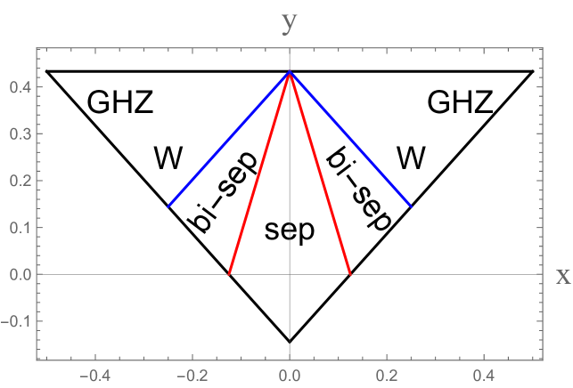
Figure 1: (Color online) Complete classification of GHZ-symmetric states.

The whole GHZ-symmetric states are represented as points inside a triangle of Fig. 1 in $x-y$ plane. Authors in Ref. elts12-1 succeeded in classifying the entanglement of the three-qubit GHZ-symmetric states completely. The result is shown in Fig. 1, where the linear hierarchy S $\subset$ B $\subset$ W $\subset$ GHZ holds in this subset states. This complete classification makes it possible to compute the three-tangle, square root of the residual entanglement, analytically for the whole GHZ-symmetric statessiewert12-1 and to construct the class-specific optimal witnesseselts12-2 . It also makes it possible to obtain lower bound of three-tangle for arbitrary three-qubit mixed stateelts13-1 . More recently, the SLOCC classification of the extended GHZ-symmetric states was discussedjung13-1 . Extended GHZ symmetry is the GHZ symmetry without qubit permutation symmetry. Thus, it is larger symmetry group than usual GHZ symmetry group, and is parametrized by four real parameters.

References	Ref. dur00	Ref. fourP-1	Ref. fourP-2	Ref. fourP-3	Ref. fourP-4	Ref. fourP-5
number of SLOCC classes	$\infty$	$9$	$8$	$23$	$49$	$9$

Table I: Number of SLOCC classes of four-qubit pure states in various references.

The SLOCC classification of the four-qubit system was explored in Ref. dur00 ; fourP-1 ; fourP-2 ; fourP-3 ; fourP-4 ; fourP-5 . Unlike, however, three-qubit case their results seem to be contradictory to each other. In particular, the number of the SLOCC classes is different as Table I shows. Furthermore, we do not know any linear hierarchy in the four-qubit system. Thus, our understanding on the four-qubit entanglement is still incomplete.

The purpose of this paper is to extend the analysis of Ref. elts12-1 to four-qubit system. For this purpose we choose nine SLOCC classes of four-qubit system suggested in Ref. fourP-1 . This classification is achieved by making use of the Jordan block structure of some complex symmetric matrix. Nine classes and their representative states are

$$G_{abcd} = \frac{a+d}{2}(|0000\rangle+|1111\rangle)+\frac{a-d}{2}(|0011\rangle+|1100\rangle)$$

$$\hskip 2.84544pt+\frac{b+c}{2}(|0101\rangle+|1010\rangle)+\frac{b-c}{2}(|0110\rangle+|1001\rangle)$$

$$L_{abc_{2}} = \frac{a+b}{2}(|0000\rangle+|1111\rangle)+\frac{a-b}{2}(|0011\rangle+|1100\rangle)$$

$$\hskip 14.22636pt+c(|0101\rangle+|1010\rangle)+|0110\rangle$$

$$L_{a_{2}b_{2}} = a(|0000\rangle+|1111\rangle)+b(|0101\rangle+|1010\rangle)+|0110\rangle+|0011\rangle$$

$$L_{ab_{3}} = a(|0000\rangle+|1111\rangle)+\frac{a+b}{2}(|0101\rangle+|1010\rangle)$$

$$\hskip 2.84544pt+\frac{a-b}{2}(|0110\rangle+|1001\rangle)+\frac{i}{\sqrt{2}}(|0001\rangle+|0010\rangle+|0111\rangle+|1011\rangle)$$

$$L_{a_{4}} = a(|0000\rangle+|0101\rangle+|1010\rangle+|1111\rangle)+(i|0001\rangle+|0110\rangle-i|1011\rangle)$$

$$L_{a_{2}0_{3\oplus\bar{1}}} = a(|0000\rangle+|1111\rangle)+(|0011\rangle+|0101\rangle+|0110\rangle)$$

$$L_{0_{5\oplus\bar{3}}} = |0000\rangle+|0101\rangle+|1000\rangle+|1110\rangle$$

$$L_{0_{7\oplus\bar{1}}} = |0000\rangle+|1011\rangle+|1101\rangle+|1110\rangle$$

$$L_{0_{3\oplus\bar{1}}0_{3\oplus\bar{1}}} = |0000\rangle+|0111\rangle,$$

where $a$, $b$, $c$, and $d$ are complex parameters with nonnegative real part.

This paper is organized as follows. In sec. II we examine the four-qubit GHZ (GHZ₄) symmetry. Unlike the three-qubit case the whole set of GHZ₄-symmetric states is parametrized by three real parameters, say $x$, $y$, and $z$. In the parameter space all GHZ₄-symmetric states can be represented as points inside a tetrahedron. In sec. III we examine a question where $L_{abc_{2}}$, $L_{a_{2}b_{2}}$, $L_{a_{2}0_{3\oplus\bar{1}}}$, $L_{0_{3\oplus\bar{1}}0_{3\oplus\bar{1}}}$, and $L_{a_{4}}$ GHZ₄-symmetric states reside in the tetrahedron, respectively. Using the results we derive the three linear hierarchies $L_{abc_{2}}\subset L_{a_{4}}\subset L_{a_{2}b_{2}}\subset G_{abcd}$, $L_{a_{2}0_{3\oplus\bar{1}}}\subset G_{abcd}$, $L_{0_{3\oplus\bar{1}}0_{3\oplus\bar{1}}}\subset G_{abcd}$ which hold, at least, in the whole set of the GHZ₄-symmetric states. Of course, these linear hierarchies are not complete because we have not analyzed other SLOCC classes ($L_{ab_{3}}$, $L_{0_{5\oplus\bar{3}}}$, $L_{0_{7\oplus\bar{1}}}$) due to various difficulties. This difficulties are discussed in sec. IV. In the same section a brief conclusion is also given. In appendices A, B, C, D, and E we present a detailed calculation of sec. III, where Lagrange multiplier technique is extensively used.

II GHZ₄ Symmetry

It is straightforward to generalize the three-qubit GHZ symmetry to higher-qubit system. The direct generalization to four-qubit system can be written as a symmetry under (i) simultaneous flips (ii) qubit permutation (iii) qubit rotations about the $z$-axis of the form

$$U(\phi_{1},\phi_{2},\phi_{3})=e^{i\phi_{1}\sigma_{z}}\otimes e^{i\phi_{2}\sigma_{z}}\otimes e^{i\phi_{3}\sigma_{z}}\otimes e^{-i(\phi_{1}+\phi_{2}+\phi_{3})\sigma_{z}}.$$ (2)

One can show that the general form of the four-qubit states invariant under the transformations (i), (ii), and (iii) is

$$\hskip 71.13188pt\rho_{4}^{S}=\beta\left[\lvert 0000\rangle\langle 1111\lvert+\lvert 1111\rangle\langle 0000\lvert\right]$$ (3)

$$+\mbox{diag}\left(\alpha_{1},\alpha_{2},\alpha_{2},\alpha_{3},\alpha_{2},\alpha_{3},\alpha_{3},\alpha_{2},\alpha_{2},\alpha_{3},\alpha_{3},\alpha_{2},\alpha_{3},\alpha_{2},\alpha_{2},\alpha_{1}\right)$$

where $\beta$, $\alpha_{1}$, $\alpha_{2}$ and $\alpha_{3}$ are real numbers satisfying $\alpha_{1}+4\alpha_{2}+3\alpha_{3}=\frac{1}{2}$. Unlike the three-qubit case, $\rho_{4}^{S}$ is represented by three real parameters.

Now, we define the three real parameters $x$, $y$, $z$, as

$$x=\beta$$ (4)

$$y=\sqrt{\frac{8}{7}}\left(\alpha_{1}-\frac{1}{16}\right)$$

$$z=\sqrt{\frac{28}{3}}\left(\frac{\alpha_{1}}{7}+\alpha_{2}-\frac{1}{14}\right).$$

Then, it is straightforward to show that the Hilbert-Schmidt metric of $\rho_{4}^{S}$ equals to the Euclidean metric, i.e.

$$d^{2}\left[\rho_{4}^{S}(\alpha_{1},\alpha_{2},\alpha_{3},\beta),\rho_{4}^{S}(\alpha_{1}^{\prime},\alpha_{2}^{\prime},\alpha_{3}^{\prime},\beta^{\prime})\right]=(x-x^{\prime})^{2}+(y-y^{\prime})^{2}+(z-z^{\prime})^{2}$$ (5)

where $d^{2}(A,B)=\frac{1}{2}\mbox{tr}(A-B)^{\dagger}(A-B)$. The four-qubit GHZ states $\lvert\mbox{GHZ}\rangle_{\pm}=(\lvert 0000\rangle+\lvert 1111\rangle)/\sqrt{2}$ correspond to $x=\pm 1/2$, $y=\sqrt{7/32}$, and $z=0$, respectively.

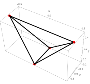
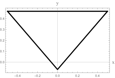
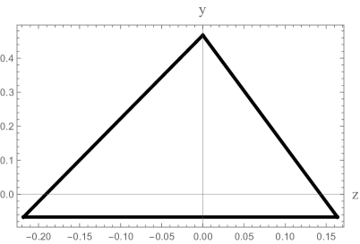
Figure 2: (Color online) (a) The restriction (6) implies that all GHZ-symmetric states (3) should lie inside the tetrahedron. (b) Projection of the tetrahedron into ($x$, $y$)-plane. (c) Projection of the tetrahedron into ($y$, $z$)-plane.

In order for $\rho_{4}^{S}$ to be a physical state we have the restrictions

$$0\leq\alpha_{2}\leq\frac{1}{8}\hskip 28.45274pt0\leq\alpha_{3}\leq\frac{1}{6}\hskip 28.45274pt0\leq\alpha_{1}\leq\frac{1}{2}\hskip 28.45274pt0\leq\alpha_{1}\pm x\leq 1.$$ (6)

Eq. (6) implies that the physical state should lie inside the tetrahedron in ($x$, $y$, $z$)-spaces as Fig. 2(a) shows. The vertices of the tetrahedron and corresponding quantum states are

$$P_{1}=\left(\frac{1}{2},\sqrt{\frac{7}{32}},0\right)\hskip 14.22636pt\lvert\mbox{GHZ}_{+}\rangle=\frac{1}{\sqrt{2}}\left(\lvert 0000\rangle+\lvert 1111\rangle\right)$$

$$P_{2}=\left(-\frac{1}{2},\sqrt{\frac{7}{32}},0\right)\hskip 14.22636pt\lvert\mbox{GHZ}_{-}\rangle=\frac{1}{\sqrt{2}}\left(\lvert 0000\rangle-\lvert 1111\rangle\right)$$

$$P_{3}=\left(0,-\frac{1}{8}\sqrt{\frac{2}{7}},-\frac{1}{\sqrt{21}}\right)$$

$$\pi_{3}=\frac{1}{6}\bigg{[}\lvert 0011\rangle\langle 0011\lvert+\lvert 0101\rangle\langle 0101\lvert+\lvert 0110\rangle\langle 0110\lvert$$ (7)

$$\hskip 56.9055pt+\lvert 1001\rangle\langle 1001\lvert+\lvert 1010\rangle\langle 1010\lvert+\lvert 1100\rangle\langle 1100\lvert\bigg{]}$$

$$P_{4}=\left(0,-\frac{1}{8}\sqrt{\frac{2}{7}},\frac{\sqrt{21}}{28}\right)$$

$$\pi_{4}=\frac{1}{8}\bigg{[}\lvert 0001\rangle\langle 0001\lvert+\lvert 0010\rangle\langle 0010\lvert+\lvert 0100\rangle\langle 0100\lvert+\lvert 0111\rangle\langle 0111\lvert$$

$$\hskip 56.9055pt+\lvert 1000\rangle\langle 1000\lvert+\lvert 1011\rangle\langle 1011\lvert+\lvert 1101\rangle\langle 1101\lvert+\lvert 1110\rangle\langle 1110\lvert\bigg{]}.$$

The origin in Fig. 2 (a) corresponds to the completely mixed state $I/16$. Eq. (6) also implies that the projections of the tetrahedron into ($x$, $y$) and ($z$, $y$) planes are Fig. 1(b) and Fig. 1(c), respectively. Thus, the physical states should reside in the triangles. It is worthwhile noting that the sign of $x$ does not change the character of entanglement because $\rho_{4}^{S}(-x,y,z)=u\rho_{4}^{S}(x,y,z)u^{\dagger}$, where $u=i\sigma_{x}\otimes\sigma_{y}\otimes\sigma_{y}\otimes\sigma_{y}$.

Like a three-qubit GHZ symmetry there is a correspondence between four-qubit pure states and four-qubit GHZ₄-symmetric states as follows. Let $\lvert\psi\rangle$ be a four-qubit pure state. Then, the corresponding GHZ₄-symmetric state $\rho_{4}^{S}(\psi)$ can be written as

$$\rho_{4}^{S}(\psi)=\int dUU\lvert\psi\rangle\langle\psi\lvert U^{\dagger}$$ (8)

where the integral is understood to cover the entire GHZ₄ symmetry group, i.e., unitaries $U(\phi_{1},\phi_{2},\phi_{3})$ in Eq. (2) and averaging over the discrete symmetries. For example, if $\lvert\psi\rangle=\sum_{i,j,k,l=0}^{1}\psi_{ijkl}\lvert ijkl\rangle$, $\rho_{4}^{S}(\psi)$ becomes Eq. (3) with

$$x=\frac{1}{2}\left[\psi_{0000}\psi_{1111}^{*}+\psi_{0000}^{*}\psi_{1111}\right]$$ (9)

$$\alpha_{1}=\frac{1}{2}\left[|\psi_{0000}|^{2}+|\psi_{1111}|^{2}\right]$$

$$\alpha_{2}=\frac{1}{8}\left[|\psi_{0001}|^{2}+|\psi_{0010}|^{2}+|\psi_{0100}|^{2}+|\psi_{1000}|^{2}+|\psi_{1110}|^{2}+|\psi_{1101}|^{2}+|\psi_{1011}|^{2}+|\psi_{0111}|^{2}\right]$$

$$\alpha_{3}=\frac{1}{6}\left[|\psi_{0011}|^{2}+|\psi_{0101}|^{2}+|\psi_{0110}|^{2}+|\psi_{1001}|^{2}+|\psi_{1010}|^{2}+|\psi_{1100}|^{2}\right].$$

Note that $\langle\psi\lvert\psi\rangle=1$ implies $2\alpha_{1}+8\alpha_{2}+6\alpha_{3}=1$.

III SLOCC classification of GHZ-symmetric states

In this section we examine a question where $L_{abc_{2}}$, $L_{a_{2}b_{2}}$, $L_{a_{2}0_{3\oplus\bar{1}}}$, $L_{0_{3\oplus\bar{1}}0_{3\oplus\bar{1}}}$, and $L_{a_{4}}$ GHZ₄-symmetric states reside in the tetrahedron of Fig. 2(a), respectively by applying the Lagrange multiplier method. The detailed calculation is presented in the five appendices. Similar issue was discussed in Ref. park14-1 . However, in this reference the full GHZ₄ symmetry was not discussed because of calculation difficulties.

III.1 $L_{abc_{2}}$

The $L_{abc_{2}}$ SLOCC classification is represented as

$$L_{abc_{2}}=\frac{a+b}{2}(|0000\rangle+|1111\rangle)+\frac{a-b}{2}(|0011\rangle+|1100\rangle)+c(|0101\rangle+|1010\rangle)+|0110\rangle$$

where $a$ and $b$ are complex parameters with nonnegative real part. In this section we want to explore a question where $L_{abc_{2}}$ GHZ₄-symmetric states reside in the tetrahedron.

The class $L_{abc_{2}}$ involves the fully separable state $\lvert 0110\rangle$ when $a=b=c=0$. In appendix A we use this state to show that when $y$ and $z$ are given, the $L_{abc_{2}}$ class of the GHZ₄-symmetric states resides in $x\leq x_{max}$, where

$$x_{max}=2\alpha_{1}\frac{u}{1+u^{2}}.$$ (10)

In Eq. (10) $u$ is a quantity satisfying the quartic equation

$$2\left[\alpha_{1}(1+u)^{2}+2\alpha_{2}(1+u^{2})\right]^{2}-\alpha_{1}(1+u^{2})(1+u)^{2}=0.$$ (11)

Eq. (11) can be solved numerically. The numerical result is presented in Fig. 3(a). The region where $L_{abc_{2}}$ GHZ₄-symmetric states reside can be described as follows. Consider a rectangle $P_{3}z_{1}z_{2}z_{3}$, where $P_{3}$ is given in Eq. (II) and

$$z_{1}=\left(\frac{1}{4},\frac{3\sqrt{14}}{56},-\frac{1}{2\sqrt{21}}\right)\hskip 14.22636ptz_{2}=\left(0,\sqrt{\frac{7}{32}},0\right)\hskip 14.22636ptz_{3}=\left(-\frac{1}{4},\frac{3\sqrt{14}}{56},-\frac{1}{2\sqrt{21}}\right).$$ (12)

Note that at these points $\alpha_{2}$ is zero. Now, bending this rectangle inward the tetrahedron, one can obtain the region where the GHZ₄-symmetric states of $L_{abc_{2}}$ reside.

Note that even though we start with the fully separable state $\lvert 0110\rangle$, this region does not coincide with the region where the PPT condition holds. Physically, this is because of the fact that $L_{abc_{2}}$ does not involve only fully separable states. It contains entangled states depending on the parameters $a$, $b$, and $c$. Mathematically, this fact arises due to the fact that $x^{\Lambda}$ in Eq. (A.10) has less symmetry due to $\Theta_{2}$ (see appendix A).

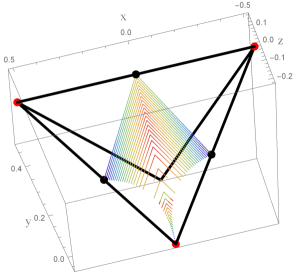
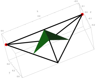
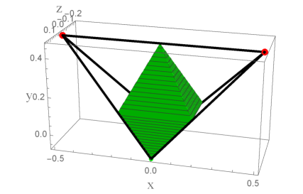
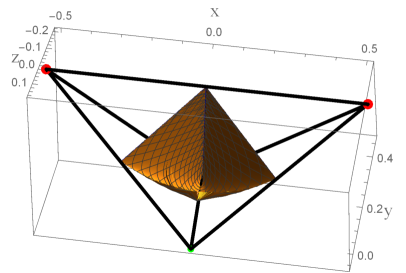
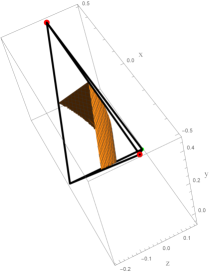
Figure 3: (Color online) The regions where the GHZ₄-symmetric states of (a) $L_{abc_{2}}$, (b) $L_{a_{2}b_{2}}$, (c) $L_{a_{2}0_{3\oplus\bar{1}}}$, (d) $L_{0_{3\oplus\bar{1}}0_{3\oplus\bar{1}}}$, (e) $L_{a_{4}}$ classes reside in the tetrahedron of Fig. 2(a).

III.2 $L_{a_{2}b_{2}}$

The $L_{a_{2}b_{2}}$ SLOCC classification is represented as

$$L_{a_{2}b_{2}}=a(|0000\rangle+|1111\rangle)+b(|0101\rangle+|1010\rangle)+|0110\rangle+|0011\rangle.$$

In this section we want to explore a question where $L_{a_{2}b_{2}}$ GHZ₄-symmetric states reside in the tetrahedron.

The class $L_{a_{2}b_{2}}$ involves the partially separable state $\lvert 0110\rangle+\lvert 0011\rangle$ when $a=b=0$. In appendix B we use this state to show that when $y$ and $z$ are given, the $L_{a_{2}b_{2}}$ class of the GHZ₄-symmetric states resides in $x\leq x_{max}$, where $x_{max}=3\alpha_{3}$. This is represented in Fig. 3(b). The remarkable fact is that the region represented by $x_{max}=3\alpha_{3}$ contains the region where $L_{abc_{2}}$ GHZ-symmetric states reside (Fig. 3(a)). This means the hierarchy $L_{abc_{2}}\subset L_{a_{2}b_{2}}$ holds, at least, in the GHZ₄-symmetric states.

III.3 $L_{a_{2}0_{3\oplus\bar{1}}}$

The $L_{a_{2}0_{3\oplus\bar{1}}}$ SLOCC classification is represented as

$$L_{a_{2}0_{3\oplus\bar{1}}}=a(|0000\rangle+|1111\rangle)+(|0011\rangle+|0101\rangle+|0110\rangle).$$

In this section we want to explore a question where $L_{a_{2}0_{3\oplus\bar{1}}}$ GHZ₄-symmetric states reside in the tetrahedron.

The class $L_{a_{2}0_{3\oplus\bar{1}}}$ involves the partially separable state $\lvert 0011\rangle+\lvert 0101\rangle+\lvert 0110\rangle$ when $a=0$. In appendix C we use this state to show that when $y$ and $z$ are given, the $L_{a_{2}0_{3\oplus\bar{1}}}$ class of the GHZ-symmetric states resides in $x\leq x_{max}$, where $x_{max}=9f\nu\mu_{1}\mu_{2}^{2}$. The four parameters $f$, $\nu$, $\mu_{1}$, and $\mu_{2}$ satisfy

$$3f(1+\nu^{2})\left[3+3\mu_{1}^{2}\mu_{2}^{4}+(\mu_{1}+2\mu_{2})^{2}+\mu_{2}^{2}(2\mu_{1}+\mu_{2})^{2}\right]=1$$

$$9f(1+\nu^{2}\mu_{1}^{2}\mu_{2}^{4})=2\alpha_{1}$$ (13)

$$3f\left[3\mu_{1}^{2}\mu_{2}^{4}+3\nu^{2}+(\mu_{1}+2\mu_{2})^{2}+\nu^{2}\mu_{2}^{2}(2\mu_{1}+\mu_{2})^{2}\right]=8\alpha_{2}$$

$$a\nu^{4}+b\nu^{2}+c=0,$$

where

$$a=(\mu_{1}+2\mu_{2})(3-2\mu_{1}\mu_{2}^{3}-\mu_{2}^{4})$$

$$b=-(\mu_{1}^{2}+\mu_{1}\mu_{2}+\mu_{2}^{2})(\mu_{1}+5\mu_{2}-5\mu_{1}\mu_{2}^{4}-\mu_{2}^{5})$$ (14)

$$c=\mu_{1}\mu_{2}^{2}(2\mu_{1}+\mu_{2})(\mu_{1}+2\mu_{2}-3\mu_{1}\mu_{2}^{4}).$$

From Eq. (III.3) one can solve $f$, $\nu$, $\mu_{1}$, and $\mu_{2}$ numerically. The region of the resulting $x_{max}$ is not convex. Thus, we should choose the convex hull, which is represented by Fig. 3(c). The region where $L_{a_{2}0_{3\oplus\bar{1}}}$ GHZ₄-symmetric states reside can be described as a polygon, whose vertices are $(0.185703,0.13171,0.102878)$, $(-0.185703,0.13171,0.102878)$, $(0,-(1/8)\sqrt{2/7},-1/\sqrt{21})$, $(0.185703,0.13171,-0.13717)$, $(-0.185703,0.13171,-0.13717)$, and $(0,\sqrt{7/32},0)$. Comparing Fig. 3(c) with Fig. 3(a) and Fig. 3(b), one can show that $L_{a_{2}0_{3\oplus\bar{1}}}$ does not have any hierarchy relation with $L_{abc_{2}}$ and $L_{a_{2}b_{2}}$.

III.4 $L_{0_{3\oplus\bar{1}}0_{3\oplus\bar{1}}}$

The $L_{0_{3\oplus\bar{1}}0_{3\oplus\bar{1}}}$ SLOCC classification is represented as

$$L_{0_{3\oplus\bar{1}}0_{3\oplus\bar{1}}}=|0000\rangle+|0111\rangle.$$

In this section we want to explore a question where $L_{0_{3\oplus\bar{1}}0_{3\oplus\bar{1}}}$ GHZ₄-symmetric states reside in the tetrahedron.

In appendix D we use this state to show that when $y$ and $z$ are given, the $L_{0_{3\oplus\bar{1}}0_{3\oplus\bar{1}}}$ class of the GHZ₄-symmetric states resides in $x\leq x_{max}$, where

$$x_{max}=\sqrt{\frac{2\alpha_{1}(1-8\alpha_{2})-(1-16\alpha_{2}+32\alpha_{2}^{2})+6\alpha_{3}\sqrt{1-16\alpha_{2}}}{2}}.$$ (15)

However, the region generated by Eq. (15) is not convex. Thus, we should choose its convex hull, which is depicted in Fig. 3(d). The region is composed of two plane triangles $z_{2}P_{3}r_{1}$ and $z_{2}P_{3}r_{2}$, and a curved surface connecting these triangles, where $z_{2}$ and $P_{3}$ are given in Eq. (12) and Eq. (II), respectively, and

$$r_{1}=\left(\frac{1}{4},\frac{3}{4\sqrt{14}},\frac{\sqrt{21}}{56}\right)\hskip 28.45274ptr_{2}=\left(-\frac{1}{4},\frac{3}{4\sqrt{14}},\frac{\sqrt{21}}{56}\right).$$ (16)

Comparing Fig. 3(d) with Fig. 3(a), Fig. 3(b) and Fig. 3(c), one can show that $L_{0_{3\oplus\bar{1}}0_{3\oplus\bar{1}}}$ does not have any hierarchy relation with $L_{abc_{2}}$, $L_{a_{2}b_{2}}$, and $L_{a_{2}0_{3\oplus\bar{1}}}$.

III.5 $L_{a_{4}}$

The $L_{a_{4}}$ SLOCC classification is represented as

$$L_{a_{4}}=a(|0000\rangle+|0101\rangle+|1010\rangle+|1111\rangle)+(i|0001\rangle+|0110\rangle-i|1011\rangle).$$

When $a=0$ this is reduced to $L_{a_{4}}=|0001\rangle+|0110\rangle-|1011\rangle$. The factor $i$ can be absorbed by redefining the second qubit as $\lvert 0\rangle\rightarrow-i\lvert 0\rangle$. If we apply $\openone\otimes\openone\otimes\sigma_{y}\otimes\sigma_{y}$ and interchanging third and fourth qubits, $L_{a_{4}}$ reduces to

$$L_{a_{4}}=|0001\rangle+|0110\rangle+|1000\rangle.$$ (17)

In this section we use this state to explore a question where $L_{a_{4}}$ GHZ₄-symmetric states reside in the tetrahedron.

In appendix E we use this state to show that when $y$ and $z$ are given, the $L_{a_{4}}$ class of the GHZ₄-symmetric states resides in $x\leq x_{max}$. where

$$x_{max}=\frac{1}{2}\left[(3\alpha_{3}-\alpha_{1})+\sqrt{\frac{\alpha_{1}+3\alpha_{3}-4\alpha_{2}}{2}}\right].$$ (18)

The region where the states of $L_{a_{4}}$-class is depicted in Fig. 3(e). Comparing this figure with other figures of Fig. 3 we can derive the linear hierarchy $L_{abc_{2}}\subset L_{a_{4}}\subset L_{a_{2}b_{2}}$, which holds, at least, in the GHZ₄-symmetric states.

IV Conclusions

In this paper we explore GHZ₄ symmetry in four-qubit system. Unlike three-qubit GHZ symmetry the whole set of the GHZ₄-symmetric states is represented by three real parameters, say $x$, $y$, and $z$. In the parameter space all GHZ₄-symmetric states reside inside the tetrahedron of Fig. 2(a).

Next, we explore a question where the given SLOCC class of the GHZ₄-symmetric states resides in the tetrahedron. Among nine SLOCC classes we have examined five classes, i.e. $L_{abc_{2}}$, $L_{a_{2}b_{2}}$, $L_{a_{2}0_{3\oplus\bar{1}}}$, $L_{0_{3\oplus\bar{1}}0_{3\oplus\bar{1}}}$, and $L_{a_{4}}$. Since the class $G_{abcd}$ involves the maximally entangled states, it should be at the top in the linear hierarchy like GHZ class in three-qubit system. Our analysis yields the following three different linear hierarchies $L_{abc_{2}}\subset L_{a_{4}}\subset L_{a_{2}b_{2}}\subset G_{abcd}$, $L_{a_{2}0_{3\oplus\bar{1}}}\subset G_{abcd}$, and $L_{0_{3\oplus\bar{1}}0_{3\oplus\bar{1}}}\subset G_{abcd}$, at least, in the whole set of the GHZ₄-symmetric states. Of course, these linear hierarchies are incomplete because we have not analyzed the SLOCC classes $L_{ab_{3}}$, $L_{0_{5\oplus\bar{3}}}$, and $L_{0_{7\oplus\bar{1}}}$ in the present paper. The reason why we have not analyzed these classes is mainly due to the following computational difficulties. The quantity $x^{\Lambda}$ defined in Eq. (A.10) in $L_{ab_{3}}$, $L_{0_{5\oplus\bar{3}}}$, and $L_{0_{7\oplus\bar{1}}}$ classes has less symmetry than that in other SLOCC classes. Thus, computation of $x_{max}$ is highly complicated because of many free parameters in the Lagrange multiplier procedure. Although we compute $x_{max}$ through numerical analysis, the resulting region in the tetrahedron becomes very complicated non-convex volume. Thus, it is highly difficult to derive the convex hull of this volume.

We hope to consider other numerical techniques, which enable us to treat the SLOCC classes $L_{ab_{3}}$, $L_{0_{5\oplus\bar{3}}}$, and $L_{0_{7\oplus\bar{1}}}$ in the future. If these techniques are available, it may lead the complete linear hierarchies in the four-qubit system.

Acknowledgement: This work was supported by the Kyungnam University Foundation Grant, 2016.

Appendix A: $L_{abc_{2}}$

In this appendix we prove Eq. (10) by applying the Lagrange multiplier method. Let us define

$$\lvert\psi\rangle=\left(\begin{array}[]{cc}A_{1}&B_{1}\\ C_{1}&D_{1}\end{array}\right)\otimes\left(\begin{array}[]{cc}A_{2}&B_{2}\\ C_{2}&D_{2}\end{array}\right)\otimes\left(\begin{array}[]{cc}A_{3}&B_{3}\\ C_{3}&D_{3}\end{array}\right)\otimes\left(\begin{array}[]{cc}A_{4}&B_{4}\\ C_{4}&D_{4}\end{array}\right)\lvert 0110\rangle.$$ (A.9)

Then, it is straightforward derive the corresponding GHZ₄-symmetric state by making use of Eq. (9). In order to derive the maximum of $x$ when $y$ and $z$ are fixed, we define $x^{\Lambda}$ as

$$x^{\Lambda}=x+\Lambda_{0}\Theta_{0}+\Lambda_{1}\Theta_{1}+\Lambda_{2}\Theta_{2},$$ (A.10)

where

$$x=(A_{1}C_{1})(B_{2}D_{2})(B_{3}D_{3})(A_{4}C_{4})$$

$$\Theta_{0}=(A_{1}^{2}+C_{1}^{2})(B_{2}^{2}+D_{2}^{2})(B_{3}^{2}+D_{3}^{2})(A_{4}^{2}+C_{4}^{2})-1$$ (A.11)

$$\Theta_{1}=\frac{1}{2}\left[(A_{1}B_{2}B_{3}A_{4})^{2}+(C_{1}D_{2}D_{3}C_{4})^{2}\right]-\alpha_{1}$$

$$\Theta_{2}=\frac{1}{8}\left[(A_{1}^{2}D_{2}^{2}+C_{1}^{2}B_{2}^{2})(B_{3}^{2}A_{4}^{2}+D_{3}^{2}C_{4}^{2})+(A_{1}^{2}B_{2}^{2}+C_{1}^{2}D_{2}^{2})(B_{3}^{2}C_{4}^{2}+D_{3}^{2}A_{4}^{2})\right]-\alpha_{2}.$$

Of course, the constraints $\Theta_{j}=0\hskip 5.69046pt(j=1,2,3)$ arise from $\langle\psi\lvert\psi\rangle=1$ and Eq. (9).

Note that $x$, $\Theta_{0}$, and $\Theta_{1}$ have $1\leftrightarrow 4$ and $2\leftrightarrow 3$ symmetries. However, this symmetry does not hold in $\Theta_{2}$. Instead, it has $(1,2)\leftrightarrow(4,3)$ symmetry. Thus, whole $x^{\Lambda}$ has $(1,2)\leftrightarrow(4,3)$ symmetry. Using this symmetry $x_{max}$, maximum of $x$, arises at $A_{1}^{2}=A_{4}^{2}\equiv a$, $C_{1}^{2}=C_{4}^{2}\equiv c$, $B_{2}^{2}=B_{3}^{2}\equiv b$, and $D_{2}^{2}=D_{4}^{2}\equiv d$. Then, $x$ and constraints become

$$x=abcd\hskip 56.9055pt\Theta_{0}=(a+c)^{2}(b+d)^{2}-1$$

$$\Theta_{1}=\frac{1}{2}(a^{2}b^{2}+c^{2}d^{2})-\alpha_{1}\hskip 28.45274pt\Theta_{2}=\frac{1}{4}(ab+cd)(ad+bc)-\alpha_{2}.$$

Now, one can derive the Lagrange equations $\frac{\partial x^{\Lambda}}{\partial z}=0\hskip 5.69046pt(z=a,b,c,d)$ explicitly. However, we do not need these equations because the constraints $\Theta_{j}=0$ fix $x$. In order to show this let us define $\mu_{1}=c/a$ and $\mu_{2}=d/c$. And we define $v=\mu_{1}+\mu_{2}$ and $u=\mu_{1}\mu_{2}$. Then, $x=(a^{2}b^{2})u$ and the constraints become

$$(a^{2}b^{2})(1+v+u)^{2}=1\hskip 14.22636pt(a^{2}b^{2})(1+u^{2})=2\alpha_{1}\hskip 14.22636pt(a^{2}b^{2})v(1+u)=4\alpha_{2}.$$ (A.13)

Eliminating $a^{2}b^{2}$ and $v$ from Eq. (A.13), one can derive Eq. (11). Also, combining Eq. (A.13) and $x=(a^{2}b^{2})u$, one can derive Eq. (10).

Appendix B : $L_{a_{2}b_{2}}$

In this appendix we prove that the $L_{a_{2}b_{2}}$ GHZ₄-symmetric states reside in the tetrahedron bounded by $x_{max}=3\alpha_{3}$ when $y$ and $z$ are fixed. Let us define

$$\lvert\psi\rangle=\left(\begin{array}[]{cc}A_{1}&B_{1}\\ C_{1}&D_{1}\end{array}\right)\otimes\left(\begin{array}[]{cc}A_{2}&B_{2}\\ C_{2}&D_{2}\end{array}\right)\otimes\left(\begin{array}[]{cc}A_{3}&B_{3}\\ C_{3}&D_{3}\end{array}\right)\otimes\left(\begin{array}[]{cc}A_{4}&B_{4}\\ C_{4}&D_{4}\end{array}\right)(\lvert 0110\rangle+\lvert 0011\rangle).$$ (B.9)

Then, the corresponding $x$ and $\alpha_{j}$ can be straightforwardly computed by making use of Eq. (9). Similar to appendix A we define $x^{\Lambda}$ as Eq. (A.10), where

$$x=A_{1}C_{1}B_{3}D_{3}(B_{2}A_{4}+A_{2}B_{4})(D_{2}C_{4}+C_{2}D_{4})$$

$$\Theta_{0}=(A_{1}^{2}+C_{1}^{2})(B_{3}^{2}+D_{3}^{2})\big{[}(B_{2}A_{4}+A_{2}B_{4})^{2}+(B_{2}C_{4}+A_{2}D_{4})^{2}$$

$$\hskip 56.9055pt+(D_{2}A_{4}+C_{2}B_{4})^{2}+(D_{2}C_{4}+C_{2}D_{4})^{2}\big{]}-1$$ (B.10)

$$\Theta_{1}=\frac{1}{2}\left[A_{1}^{2}B_{3}^{2}(B_{2}A_{4}+A_{2}B_{4})^{2}+C_{1}^{2}D_{3}^{2}(D_{2}C_{4}+C_{2}D_{4})^{2}\right]-\alpha_{1}$$

$$\Theta_{2}=\frac{1}{8}\Bigg{[}(A_{1}^{2}B_{3}^{2}+C_{1}^{2}D_{3}^{2})\left\{(B_{2}C_{4}+A_{2}D_{4})^{2}+(D_{2}A_{4}+C_{2}B_{4})^{2}\right\}$$

$$\hskip 56.9055pt+(A_{1}^{2}D_{3}^{2}+C_{1}^{2}B_{3}^{2})\left\{(B_{2}A_{4}+A_{2}B_{4})^{2}+(D_{2}C_{4}+C_{2}D_{4})^{2}\right\}\bigg{]}-\alpha_{2}.$$

Since $x^{\Lambda}$ has $2\leftrightarrow 4$ symmetry, the maximum of $x$ occurs when $A_{2}=A_{4}\equiv A$, $B_{2}=B_{4}\equiv B$, $C_{2}=C_{4}\equiv C$, and $D_{2}=D_{4}\equiv D$. Defining $\mu_{1}=AB$, $\mu_{2}=CD$, and $\mu_{3}=AD+BC$, one can show that Eq. (Greenberger-Horne-Zeilinger Symmetry in Four Qubit System) reduce to

$$x=4A_{1}C_{1}B_{3}D_{3}\mu_{1}\mu_{2}$$

$$\Theta_{0}=2(A_{1}^{2}+C_{1}^{2})(B_{3}^{2}+D_{3}^{2})(2\mu_{1}^{2}+2\mu_{2}^{2}+\mu_{3}^{2})-1$$ (B.11)

$$\Theta_{1}=2\left[A_{1}^{2}B_{3}^{2}\mu_{1}^{2}+C_{1}^{2}D_{3}^{2}\mu_{2}^{2}\right]-\alpha_{1}$$

$$\Theta_{2}=\frac{1}{4}\left[(A_{1}^{2}B_{3}^{2}+C_{1}^{2}D_{3}^{2})\mu_{3}^{2}+2(A_{1}^{2}D_{3}^{2}+C_{1}^{2}B_{3}^{2})(\mu_{1}^{2}+\mu_{2}^{2})\right]-\alpha_{2}.$$

Thus, we have seven Lagrange multiplier equations $\frac{\partial x^{\Lambda}}{\partial z}=0\hskip 5.69046pt(z=\mu_{3},\mu_{1},\mu_{2},A_{1},C_{1},B_{3},D_{3})$ and three constraints $\Theta_{j}=0\hskip 5.69046pt(j=0,1,2)$. Among them $\frac{\partial x^{\Lambda}}{\partial\mu_{3}}=0$ is solved by $\mu_{3}=0$. Using this solution, one can solve the remaining Lagrange multiplier equations. Finally, one can show that the Lagrange multiplier constants can be expressed in terms of the following ratios

$$g\equiv\frac{\mu_{2}}{\mu_{1}}\hskip 14.22636ptr_{1}\equiv\frac{C_{1}}{A_{1}}\hskip 14.22636ptr_{2}\equiv\frac{D_{3}}{B_{3}}.$$ (B.12)

The explicit form of the Lagrange multiplier constants are

$$\Lambda_{0}=\frac{r_{2}(1-g^{2}r_{1}^{2}r_{2}^{2})(g^{2}r_{2}^{2}-r_{1}^{2})}{2g(1+g^{2})r_{1}(1-r_{2}^{4})(1-r_{1}^{2}r_{2}^{2})}$$

$$\Lambda_{1}=\frac{(1-g^{2})r_{1}r_{2}}{g(1-r_{1}^{2}r_{2}^{2})}$$ (B.13)

$$\Lambda_{2}=\frac{4r_{2}(r_{1}^{2}-g^{2})(1-g^{2}r_{1}^{2}r_{2}^{2})}{g(1+g^{2})r_{1}(1-r_{2}^{2})(1-r_{1}^{2}r_{2}^{2})}.$$

Inserting Eq. (Greenberger-Horne-Zeilinger Symmetry in Four Qubit System) into the remaining Lagrange multiplier equations, one can show that all equation is solved by $g=r_{1}r_{2}$. In terms of the ratios Eq. (Greenberger-Horne-Zeilinger Symmetry in Four Qubit System) becomes

$$x=4(A_{1}^{2}B_{3}^{2}\mu_{1}^{2})gr_{1}r_{2}$$

$$\Theta_{0}=0:\hskip 5.69046pt 4(A_{1}^{2}B_{3}^{2}\mu_{1}^{2})(1+r_{1}^{2})(1+r_{2}^{2})(1+g^{2})=1$$ (B.14)

$$\Theta_{1}=0:\hskip 5.69046pt 2(A_{1}^{2}B_{3}^{2}\mu_{1}^{2})(1+g^{2}r_{1}^{2}r_{2}^{2})=\alpha_{1}$$

$$\Theta_{2}=0:\hskip 5.69046pt (A_{1}^{2}B_{3}^{2}\mu_{1}^{2})(1+g^{2})(r_{1}^{2}+r_{2}^{2})=2\alpha_{2}.$$

When $g=r_{1}r_{2}$, one can show easily from Eq. (Greenberger-Horne-Zeilinger Symmetry in Four Qubit System) that $x_{max}$ becomes

$$x_{max}=\frac{1}{2}(1-2\alpha_{1}-8\alpha_{2})=3\alpha_{3}.$$ (B.15)

Of course, there are many other solutions of the Lagrange multiplier equations. However, the resulting $x_{max}$ generated by other solutions are not physical. For example, Eq. (Greenberger-Horne-Zeilinger Symmetry in Four Qubit System) with $g=1/(r_{1}r_{2})$ also solve the Lagrange multiplier equations. In this case, $x_{max}$ becomes $x_{max}=\alpha_{1}$. This means that all states in the tetrahedron are $L_{a_{2}b_{2}}$-class. Since, however, $\lvert\mbox{GHZ}_{\pm}\rangle$ are not $L_{a_{2}b_{2}}$-class evidently, this solution is unphysical.

Appendix C : $L_{a_{2}0_{3\oplus\bar{1}}}$

In this appendix we prove that the $L_{a_{2}0_{3\oplus\bar{1}}}$ GHZ₄-symmetric states reside in the tetrahedron bounded by Eq. (III.3).Let us define

$$\lvert\psi\rangle$$ (C.1)

$$=\left(\begin{array}[]{cc}A_{1}&B_{1}\\ C_{1}&D_{1}\end{array}\right)\otimes\left(\begin{array}[]{cc}A_{2}&B_{2}\\ C_{2}&D_{2}\end{array}\right)\otimes\left(\begin{array}[]{cc}A_{3}&B_{3}\\ C_{3}&D_{3}\end{array}\right)\otimes\left(\begin{array}[]{cc}A_{4}&B_{4}\\ C_{4}&D_{4}\end{array}\right)(\lvert 0011\rangle+\lvert 0101\rangle+\lvert 0110\rangle).$$ (C.10)

Then, the corresponding $x$ and $\alpha_{j}$ can be computed by using Eq. (9). Now, we define $x^{\Lambda}$ as Eq. (A.10), where

$$x=A_{1}C_{1}(A_{2}B_{3}B_{4}+B_{2}A_{3}B_{4}+B_{2}B_{3}A_{4})(C_{2}D_{3}D_{4}+D_{2}C_{3}D_{4}+D_{2}D_{3}C_{4})$$

$$\Theta_{0}=(A_{1}^{2}+C_{1}^{2})\Bigg{[}(A_{2}B_{3}B_{4}+B_{2}A_{3}B_{4}+B_{2}B_{3}A_{4})^{2}+(A_{2}B_{3}D_{4}+B_{2}A_{3}D_{4}+B_{2}B_{3}C_{4})^{2}$$

$$\hskip 56.9055pt+(A_{2}D_{3}B_{4}+B_{2}C_{3}B_{4}+B_{2}D_{3}A_{4})^{2}+(A_{2}D_{3}D_{4}+B_{2}C_{3}D_{4}+B_{2}D_{3}C_{4})^{2}$$

$$\hskip 56.9055pt+(C_{2}B_{3}B_{4}+D_{2}A_{3}B_{4}+D_{2}B_{3}A_{4})^{2}+(C_{2}B_{3}D_{4}+D_{2}A_{3}D_{4}+D_{2}B_{3}C_{4})^{2}$$

$$\hskip 28.45274pt+(C_{2}D_{3}B_{4}+D_{2}C_{3}B_{4}+D_{2}D_{3}A_{4})^{2}+(C_{2}D_{3}D_{4}+D_{2}C_{3}D_{4}+D_{2}D_{3}C_{4})^{2}\Bigg{]}-1$$ (C.11)

$$\Theta_{1}=\frac{1}{2}\left[A_{1}^{2}(A_{2}B_{3}B_{4}+B_{2}A_{3}B_{4}+B_{2}B_{3}A_{4})^{2}+C_{1}^{2}(C_{2}D_{3}D_{4}+D_{2}C_{3}D_{4}+D_{2}D_{3}C_{4})^{2}\right]-\alpha_{1}$$

$$\Theta_{2}=\frac{1}{8}\bigg{[}A_{1}^{2}(A_{2}B_{3}D_{4}+B_{2}A_{3}D_{4}+B_{2}B_{3}C_{4})^{2}+A_{1}^{2}(A_{2}D_{3}B_{4}+B_{2}C_{3}B_{4}+B_{2}D_{3}A_{4})^{2}$$

$$\hskip 42.67912pt+A_{1}^{2}(C_{2}B_{3}B_{4}+D_{2}A_{3}B_{4}+D_{2}B_{3}A_{4})^{2}+A_{1}^{2}(C_{2}D_{3}D_{4}+D_{2}C_{3}D_{4}+D_{2}D_{3}C_{4})^{2}$$

$$\hskip 42.67912pt+C_{1}^{2}(A_{2}B_{3}B_{4}+B_{2}A_{3}B_{4}+B_{2}B_{3}A_{4})^{2}+C_{1}^{2}(A_{2}D_{3}D_{4}+B_{2}C_{3}D_{4}+B_{2}D_{3}C_{4})^{2}$$

$$\hskip 28.45274pt+C_{1}^{2}(C_{2}B_{3}D_{4}+D_{2}A_{3}D_{4}+D_{2}B_{3}C_{4})^{2}+C_{1}^{2}(C_{2}D_{3}B_{4}+D_{2}C_{3}B_{4}+D_{2}D_{3}A_{4})^{2}\Bigg{]}-\alpha_{2}.$$

Since $x^{\Lambda}$ has $2\leftrightarrow 3$, $2\leftrightarrow 4$, and $3\leftrightarrow 4$ symmetries, the maximum of $x$ should occur at $A_{2}=A_{3}=A_{4}\equiv A$, $B_{2}=B_{3}=B_{4}\equiv B$, $C_{2}=C_{3}=C_{4}\equiv C$, and $D_{2}=D_{3}=D_{4}\equiv D$. Then, Eq. (Greenberger-Horne-Zeilinger Symmetry in Four Qubit System) reduces to

$$x=9A_{1}C_{1}AB^{2}CD^{2}$$ (C.12)

$$\Theta_{0}=3(A_{1}^{2}+C_{1}^{2})\left[3A^{2}B^{4}+3C^{2}D^{4}+B^{2}(2AD+BC)^{2}+D^{2}(AD+2BC)^{2}\right]-1$$

$$\Theta_{1}=\frac{9}{2}\left[A_{1}^{2}A^{2}B^{4}+C_{1}^{2}C^{2}D^{4}\right]-\alpha_{1}$$

$$\Theta_{2}=\frac{3}{8}\left[3A_{1}^{2}C^{2}D^{4}+3C_{1}^{2}A^{2}B^{4}+A_{1}^{2}B^{2}(2AD+BC)^{2}+C_{1}^{2}D^{2}(AD+2BC)^{2}\right]-\alpha_{2}.$$

Thus, we have six Lagrange multiplier equations $\frac{\partial x^{\Lambda}}{\partial z}=0\hskip 5.69046pt(z=A_{1},C_{1},A,B,C,D)$ and three constraints $\Theta_{j}=0\hskip 5.69046pt(j=0,1,2)$. The six Lagrange multiplier equations are not all independent. Now, we define

$$\mu_{1}=\frac{C}{A}\hskip 28.45274pt\mu_{2}=\frac{D}{B}\hskip 28.45274pt\nu=\frac{C_{1}}{A_{1}}.$$ (C.13)

Then, $x$ and $\Theta_{j}=0$ becomes

$$x=9f\nu\mu_{1}\mu_{2}^{2}$$

$$3f(1+\nu^{2})\left[3+3\mu_{1}^{2}\mu_{2}^{4}+(\mu_{1}+2\mu_{2})^{2}+\mu_{2}^{2}(2\mu_{1}+\mu_{2})^{2}\right]=1$$ (C.14)

$$9f(1+\nu^{2}\mu_{1}^{2}\mu_{2}^{4})=2\alpha_{1}$$

$$3f\left[3\mu_{1}^{2}\mu_{2}^{4}+3\nu^{2}+(\mu_{1}+2\mu_{2})^{2}+\nu^{2}\mu_{2}^{2}(2\mu_{1}+\mu_{2})^{2}\right]=8\alpha_{2}.$$

where $f=A_{1}^{2}A^{2}B^{4}$. Eliminating $\Lambda_{1}$, one can derive the following two equations from the Lagrange multiplier:

$$2\Lambda_{0}\beta_{1}+\frac{\Lambda_{2}}{4}\beta_{2}=0\hskip 28.45274pt2\Lambda_{0}\beta_{3}+\frac{\Lambda_{2}}{4}\beta_{4}=0,$$ (C.15)

where

$$\beta_{1}=(1+\nu^{2})\left[(\mu_{1}+2\mu_{2})+\mu_{2}^{2}(2\mu_{1}+\mu_{2})\right]$$

$$\beta_{2}=(\mu_{1}+2\mu_{2})+\nu^{2}\mu_{2}^{2}(2\mu_{1}+\mu_{2})$$ (C.16)

$$\beta_{3}=-\mu_{1}\left\{(\mu_{1}+2\mu_{2})+2\mu_{2}^{2}(2\mu_{1}+\mu_{2})+3\mu_{1}\mu_{2}^{4}\right\}+\nu^{2}\left\{3+2\mu_{2}(\mu_{1}+2\mu_{2})+\mu_{2}^{3}(2\mu_{1}+\mu_{2})\right\}$$

$$\beta_{4}=-\mu_{1}(3\mu_{1}\mu_{2}^{4}+\mu_{1}+2\mu_{2})+\nu^{2}(3+2\mu_{1}\mu_{2}^{3}+\mu_{2}^{4}).$$

Thus, the secular equation $\beta_{1}\beta_{4}-\beta_{2}\beta_{3}=0$ becomes $a\nu^{4}+b\nu^{2}+c=0$, where the coefficients $a$, $b$, and $c$ are given in Eq. (III.3).

Appendix D

In this appendix we prove Eq. (15) by applying the Lagrange multiplier method. Let us define

$$\lvert\psi\rangle=\left(\begin{array}[]{cc}A_{1}&B_{1}\\ C_{1}&D_{1}\end{array}\right)\otimes\left(\begin{array}[]{cc}A_{2}&B_{2}\\ C_{2}&D_{2}\end{array}\right)\otimes\left(\begin{array}[]{cc}A_{3}&B_{3}\\ C_{3}&D_{3}\end{array}\right)\otimes\left(\begin{array}[]{cc}A_{4}&B_{4}\\ C_{4}&D_{4}\end{array}\right)(\lvert 0000\rangle+\lvert 0111\rangle).$$ (D.1)

Then, it is straightforward derive the corresponding GHZ₄-symmetric state by making use of Eq. (9). In order to apply the Lagrange multiplier method we define $x^{\Lambda}$ as Eq. (A.10) with

$$x=A_{1}C_{1}(A_{2}A_{3}A_{4}+B_{2}B_{3}B_{4})(C_{2}C_{3}C_{4}+D_{2}D_{3}D_{4})$$

$$\Theta_{0}=(A_{1}^{2}+C_{1}^{2})\bigg{[}(A_{2}A_{3}A_{4}+B_{2}B_{3}B_{4})^{2}+(A_{2}A_{3}C_{4}+B_{2}B_{3}D_{4})^{2}+(A_{2}C_{3}A_{4}+B_{2}D_{3}B_{4})^{2}$$

$$\hskip 85.35826pt+(A_{2}C_{3}C_{4}+B_{2}D_{3}D_{4})^{2}+(C_{2}A_{3}A_{4}+D_{2}B_{3}B_{4})^{2}+(C_{2}A_{3}C_{4}+D_{2}B_{3}D_{4})^{2}$$

$$\hskip 113.81102pt+(C_{2}C_{3}A_{4}+D_{2}D_{3}B_{4})^{2}+(C_{2}C_{3}C_{4}+D_{2}D_{3}D_{4})^{2}\bigg{]}-1$$ (D.2)

$$\Theta_{1}=\frac{1}{2}\left[A_{1}^{2}(A_{2}A_{3}A_{4}+B_{2}B_{3}B_{4})^{2}+C_{1}^{2}(C_{2}C_{3}C_{4}+D_{2}D_{3}D_{4})^{2}\right]-\alpha_{1}$$

$$\Theta_{2}=\frac{1}{8}\bigg{[}A_{1}^{2}(A_{2}A_{3}C_{4}+B_{2}B_{3}D_{4})^{2}+A_{1}^{2}(A_{2}C_{3}A_{4}+B_{2}D_{3}B_{4})^{2}+A_{1}^{2}(C_{2}A_{3}A_{4}+D_{2}B_{3}B_{4})^{2}$$

$$\hskip 42.67912pt+A_{1}^{2}(C_{2}C_{3}C_{4}+D_{2}D_{3}D_{4})^{2}+C_{1}^{2}(A_{2}A_{3}A_{4}+B_{2}B_{3}B_{4})^{2}+C_{1}^{2}(A_{2}C_{3}C_{4}+B_{2}D_{3}D_{4})^{2}$$

$$\hskip 85.35826pt+C_{1}^{2}(C_{2}A_{3}C_{4}+D_{2}B_{3}D_{4})^{2}+C_{1}^{2}(C_{2}C_{3}A_{4}+D_{2}D_{3}B_{4})^{2}\bigg{]}-\alpha_{2}.$$

Since $x^{\Lambda}$ has $2\leftrightarrow 3$, $2\leftrightarrow 4$, and $3\leftrightarrow 4$ symmetries, the maximum of $x$ should occur at $A_{2}=A_{3}=A_{4}\equiv A$, $B_{2}=B_{3}=B_{4}\equiv B$, $C_{2}=C_{3}=C_{4}\equiv C$, and $D_{2}=D_{3}=D_{4}\equiv D$. Then, Eq. (Greenberger-Horne-Zeilinger Symmetry in Four Qubit System) becomes

$$x=A_{1}C_{1}(A^{3}+B^{3})(C^{3}+D^{3})$$

$$\Theta_{0}=(A_{1}^{2}+C_{1}^{2})\bigg{[}(A^{3}+B^{3})^{2}+3(A^{2}C+B^{2}D)^{2}$$

$$\hskip 113.81102pt+3(AC^{2}+BD^{2})^{2}+(C^{3}+D^{3})^{2}\bigg{]}-1$$ (D.3)

$$\Theta_{1}=\frac{1}{2}\left[A_{1}^{2}(A^{3}+B^{3})^{2}+C_{1}^{2}(C^{3}+D^{3})^{2}\right]-\alpha_{1}$$

$$\Theta_{2}=\frac{1}{8}\bigg{[}3A_{1}^{2}(A^{2}C+B^{2}D)^{2}+A_{1}^{2}(C^{3}+D^{3})^{2}$$

$$\hskip 85.35826pt+3C_{1}^{2}(AC^{2}+BD^{2})^{2}+C_{1}^{2}(A^{3}+B^{3})^{2}\bigg{]}-\alpha_{2}.$$

Thus, we have six Lagrange multiplier equations $\frac{\partial x^{\Lambda}}{\partial z}=0\hskip 5.69046pt(z=A_{1},C_{1},A,B,C,D)$. Eliminating the Lagrange multiplier constants $\Lambda_{j}$, one can derive two relations $A^{2}C+B^{2}D=0$ and $AC^{2}+BD^{2}=0$.

Since both equations gives same $x_{max}$, we consider only $A^{2}C+B^{2}D=0$ in this appendix. This is solved by $C=-\mu^{2}D$ and $B=\mu A$. Defining $\nu=C_{1}/A_{1}$ and $\rho=D/A$, one can re-express the four independent Lagrange multiplier equations in terms of $\mu$, $\nu$, and $\rho$:

$$\nu\rho^{3}(1-\mu^{3})+2\Lambda_{0}\left[1+3\rho^{4}\mu^{2}+\rho^{6}(1-\mu^{3})^{2}\right]+\Lambda_{1}+\frac{\Lambda_{2}}{4}\rho^{6}(1-\mu^{3})^{2}=0$$ (D.4)

$$\rho^{3}(1-\mu^{3})+2\Lambda_{0}\nu\left[1+3\rho^{4}\mu^{2}+\rho^{6}(1-\mu^{3})^{2}\right]+\Lambda_{1}\nu\rho^{6}(1-\mu^{3})^{2}+\frac{\Lambda_{2}}{4}\nu(1+3\rho^{4}\mu^{2})=0$$

$$\nu\rho^{3}(1-\mu^{3})+2\Lambda_{0}(1+\nu^{2})(1+\rho^{4}\mu^{5})+\Lambda_{1}+\frac{\Lambda_{2}}{4}\nu^{2}(1+\rho^{4}\mu^{5})=0$$

$$\nu\mu+2\Lambda_{0}(1+\nu^{2})\left[-2\rho+\rho^{3}\mu(1-\mu^{3})\right]+\Lambda_{1}\nu^{2}\rho^{3}\mu(1-\mu^{3})+\frac{\Lambda_{2}}{4}\left[\rho^{3}\mu(1-\mu^{3})-2\nu^{2}\rho\right]=0.$$

Three of Eq. (D.4) can be used to derive the Lagrange multiplier constants. Since their explicit forms are lengthy, we do not present in this appendix. Eliminating all Lagrange multiplier constants from Eq. (D.4), one can derive a relation

$$\rho^{6}(1-\mu^{2})^{2}=\nu^{2}(1+3\mu^{2}\rho^{4}).$$ (D.5)

In terms of $\mu$, $\nu$, and $\rho$, $x$ and $\Theta_{j}=0$ reduce to

$$x=f(1+\mu^{3})^{2}\nu\rho^{3}(1-\mu^{3})$$

$$f(1+\mu^{3})^{2}\frac{(1+\nu^{2})^{2}}{\nu^{2}}\rho^{6}(1-\mu^{3})^{2}=1$$ (D.6)

$$f(1+\mu^{3})^{2}\left[1+\nu^{2}\rho^{6}(1-\mu^{3})^{2}\right]=2\alpha_{1}$$

$$f(1+\mu^{3})^{2}\rho^{6}(1-\mu^{3})^{2}=4\alpha_{2},$$

where $f=A_{1}^{2}A^{6}$. Combining Eq. (D.5) and Eq. (Greenberger-Horne-Zeilinger Symmetry in Four Qubit System), one can derive Eq. (15) straightforwardly.

Appendix E

In this appendix we prove Eq. (18) by applying the Lagrange multiplier method. Let us define

$$\lvert\psi\rangle=\left(\begin{array}[]{cc}A_{1}&B_{1}\\ C_{1}&D_{1}\end{array}\right)\otimes\left(\begin{array}[]{cc}A_{2}&B_{2}\\ C_{2}&D_{2}\end{array}\right)\otimes\left(\begin{array}[]{cc}A_{3}&B_{3}\\ C_{3}&D_{3}\end{array}\right)\otimes\left(\begin{array}[]{cc}A_{4}&B_{4}\\ C_{4}&D_{4}\end{array}\right)(\lvert 0001\rangle+\lvert 0111\rangle+\lvert 1000\rangle).$$ (E.1)

Then, it is straightforward derive the corresponding GHZ₄-symmetric state by making use of Eq. (9). In order to apply the Lagrange multiplier method we define $x^{\Lambda}$ as Eq. (A.10) with

$$x=(A_{1}A_{2}A_{3}B_{4}+A_{1}B_{2}B_{3}A_{4}+B_{1}A_{2}A_{3}A_{4})(C_{1}C_{2}C_{3}D_{4}+C_{1}D_{2}D_{3}C_{4}+D_{1}C_{2}C_{3}C_{4})$$

$$\Theta_{0}=\bigg{[}(A_{1}A_{2}A_{3}B_{4}+A_{1}B_{2}B_{3}A_{4}+B_{1}A_{2}A_{3}A_{4})^{2}+(C_{1}A_{2}A_{3}B_{4}+C_{1}B_{2}B_{3}A_{4}+D_{1}A_{2}A_{3}A_{4})^{2}$$

$$\hskip 31.2982pt+(A_{1}A_{2}A_{3}D_{4}+A_{1}B_{2}B_{3}C_{4}+B_{1}A_{2}A_{3}C_{4})^{2}+(C_{1}A_{2}A_{3}D_{4}+C_{1}B_{2}B_{3}C_{4}+D_{1}A_{2}A_{3}C_{4})^{2}$$

$$\hskip 31.2982pt+(A_{1}A_{2}C_{3}B_{4}+A_{1}B_{2}D_{3}A_{4}+B_{1}A_{2}C_{3}A_{4})^{2}+(C_{1}A_{2}C_{3}B_{4}+C_{1}B_{2}D_{3}A_{4}+D_{1}A_{2}C_{3}A_{4})^{2}$$

$$\hskip 31.2982pt+(A_{1}A_{2}C_{3}D_{4}+A_{1}B_{2}D_{3}C_{4}+B_{1}A_{2}C_{3}C_{4})^{2}+(C_{1}A_{2}C_{3}D_{4}+C_{1}B_{2}D_{3}C_{4}+D_{1}A_{2}C_{3}C_{4})^{2}$$

$$\hskip 31.2982pt+(A_{1}C_{2}A_{3}B_{4}+A_{1}D_{2}B_{3}A_{4}+B_{1}C_{2}A_{3}A_{4})^{2}+(C_{1}C_{2}A_{3}B_{4}+C_{1}D_{2}B_{3}A_{4}+D_{1}C_{2}A_{3}A_{4})^{2}$$

$$\hskip 31.2982pt+(A_{1}C_{2}A_{3}D_{4}+A_{1}D_{2}B_{3}C_{4}+B_{1}C_{2}A_{3}C_{4})^{2}+(C_{1}C_{2}A_{3}D_{4}+C_{1}D_{2}B_{3}C_{4}+D_{1}C_{2}A_{3}C_{4})^{2}$$

$$\hskip 31.2982pt+(A_{1}C_{2}C_{3}B_{4}+A_{1}D_{2}D_{3}A_{4}+B_{1}C_{2}C_{3}A_{4})^{2}+(C_{1}C_{2}C_{3}B_{4}+C_{1}D_{2}D_{3}A_{4}+D_{1}C_{2}C_{3}A_{4})^{2}$$

$$\hskip 31.2982pt+(A_{1}C_{2}C_{3}D_{4}+A_{1}D_{2}D_{3}C_{4}+B_{1}C_{2}C_{3}C_{4})^{2}+(C_{1}C_{2}C_{3}D_{4}+C_{1}D_{2}D_{3}C_{4}+D_{1}C_{2}C_{3}C_{4})^{2}\bigg{]}$$

$$\hskip 284.52756pt-1$$ (E.2)

$$\Theta_{1}=\frac{1}{2}\left[(A_{1}A_{2}A_{3}B_{4}+A_{1}B_{2}B_{3}A_{4}+B_{1}A_{2}A_{3}A_{4})^{2}+(C_{1}C_{2}C_{3}D_{4}+C_{1}D_{2}D_{3}C_{4}+D_{1}C_{2}C_{3}C_{4})^{2}\right]$$

$$\hskip 284.52756pt-\alpha_{1}$$

$$\Theta_{2}=\frac{1}{8}\bigg{[}(A_{1}A_{2}A_{3}D_{4}+A_{1}B_{2}B_{3}C_{4}+B_{1}A_{2}A_{3}C_{4})^{2}+(A_{1}A_{2}C_{3}B_{4}+A_{1}B_{2}D_{3}A_{4}+B_{1}A_{2}C_{3}A_{4})^{2}$$

$$\hskip 31.2982pt+(A_{1}C_{2}A_{3}B_{4}+A_{1}D_{2}B_{3}A_{4}+B_{1}C_{2}A_{3}A_{4})^{2}+(A_{1}C_{2}C_{3}D_{4}+A_{1}D_{2}D_{3}C_{4}+B_{1}C_{2}C_{3}C_{4})^{2}$$

$$\hskip 31.2982pt+(C_{1}A_{2}A_{3}B_{4}+C_{1}B_{2}B_{3}A_{4}+D_{1}A_{2}A_{3}A_{4})^{2}+(C_{1}A_{2}C_{3}D_{4}+C_{1}B_{2}D_{3}C_{4}+D_{1}A_{2}C_{3}C_{4})^{2}$$

$$\hskip 31.2982pt+(C_{1}C_{2}A_{3}D_{4}+C_{1}D_{2}B_{3}C_{4}+D_{1}C_{2}A_{3}C_{4})^{2}+(C_{1}C_{2}C_{3}B_{4}+C_{1}D_{2}D_{3}A_{4}+D_{1}C_{2}C_{3}A_{4})^{2}\bigg{]}$$

$$\hskip 284.52756pt-\alpha_{2}.$$

Since $x^{\Lambda}$ has $2\leftrightarrow 3$ and $1\leftrightarrow 4$ symmetries, the maximum of $x$ should occur at

$$A_{1}=A_{4}\equiv A\hskip 28.45274ptB_{1}=B_{4}\equiv B\hskip 28.45274ptC_{1}=C_{4}\equiv C\hskip 28.45274ptD_{1}=D_{4}\equiv D$$ (E.3)

$$A_{2}=A_{3}\equiv\alpha\hskip 28.45274ptB_{2}=B_{3}\equiv\beta\hskip 28.45274ptC_{2}=C_{3}\equiv\gamma\hskip 28.45274ptD_{2}=D_{3}\equiv\delta.$$

Further, we define

$$\mu_{1}\equiv\frac{B}{A}\hskip 28.45274pt\mu_{2}\equiv\frac{D}{C}\hskip 28.45274pt\nu_{1}\equiv\frac{\beta}{\alpha}\hskip 28.45274pt\nu_{2}=\frac{\delta}{\gamma}.$$ (E.4)

Then, $x$ and $\Theta_{j}$ become

$$x=(AC\alpha\gamma)^{2}(2\mu_{1}+\nu_{1}^{2})(2\mu_{2}+\nu_{2}^{2})$$

$$\Theta_{0}=\left[A^{4}\gamma^{4}(2\mu_{1}+\nu_{2}^{2})^{2}+C^{4}\alpha^{4}(2\mu_{2}+\nu_{1}^{2})^{2}+4A^{2}C^{2}\alpha^{2}\gamma^{2}(\mu_{1}+\mu_{2}+\nu_{1}\nu_{2})^{2}\right]-6\alpha_{3}$$

$$\Theta_{1}=\left[A^{4}\alpha^{4}(2\mu_{1}+\nu_{1}^{2})^{2}+C^{4}\gamma^{4}(2\mu_{2}+\nu_{2}^{2})^{2}\right]-2\alpha_{1}$$ (E.5)

$$\Theta_{2}=\bigg{[}A^{4}\alpha^{2}\gamma^{2}(2\mu_{1}+\nu_{1}\nu_{2})^{2}+C^{4}\alpha^{2}\gamma^{2}(2\mu_{2}+\nu_{1}\nu_{2})^{2}$$

$$\hskip 85.35826pt+A^{2}C^{2}\alpha^{4}(\mu_{1}+\mu_{2}+\nu_{1}^{2})^{2}+A^{2}C^{2}\gamma^{4}(\mu_{1}+\mu_{2}+\nu_{2}^{2})^{2}\bigg{]}-4\alpha_{2}.$$

In Eq. (Greenberger-Horne-Zeilinger Symmetry in Four Qubit System) the constraint $\Theta_{0}$ is simplified by making use of $\Theta_{1}=0$, $\Theta_{2}=0$, and $2\alpha_{1}+8\alpha_{2}+6\alpha_{3}=1$. If one defines again $a\equiv A^{2}$, $b\equiv B^{2}$, $c\equiv\alpha^{2}$, and $d=\gamma^{2}$, Eq. (Greenberger-Horne-Zeilinger Symmetry in Four Qubit System) reduces to

$$x=abcd(2\mu_{1}+\nu_{1}^{2})(2\mu_{2}+\nu_{2}^{2})$$ (E.6)

$$\Theta_{0}=\left[a^{2}d^{2}(2\mu_{1}+\nu_{2}^{2})^{2}+b^{2}c^{2}(2\mu_{2}+\nu_{1}^{2})^{2}+4abcd(\mu_{1}+\mu_{2}+\nu_{1}\nu_{2})^{2}\right]-6\alpha_{3}$$

$$\Theta_{1}=a^{2}c^{2}(2\mu_{1}+\nu_{1}^{2})^{2}+b^{2}d^{2}(2\mu_{2}+\nu_{2}^{2})^{2}-2\alpha_{1}$$

$$\Theta_{2}=\bigg{[}a^{2}cd(2\mu_{1}+\nu_{1}\nu_{2})^{2}+b^{2}cd(2\mu_{2}+\nu_{1}\nu_{2})^{2}$$

$$\hskip 85.35826pt+abc^{2}(\mu_{1}+\mu_{2}+\nu_{1}^{2})^{2}+abd^{2}(\mu_{1}+\mu_{2}+\nu_{2}^{2})^{2}\bigg{]}-4\alpha_{2}.$$

Now, one can derive eight Lagrange multiplier equations $\frac{\partial x^{\Lambda}}{\partial z}=0\hskip 5.69046pt(z=a,b,c,d,\mu_{1},\mu_{2},\nu_{1},\nu_{2})$. From first four equations $(z=a,b,c,d)$, one can derive the Lagrange multiplier constants;

$$2\Lambda_{0}=\frac{\Delta_{1}}{\Delta}bcd(2\mu_{1}+\nu_{1}^{2})(2\mu_{2}+\nu_{2}^{2})(ab\omega_{2}-cd\omega_{1})$$

$$2\Lambda_{1}=-\frac{\Delta_{2}}{\Delta}bcd(2\mu_{1}+\nu_{1}^{2})(2\mu_{2}+\nu_{2}^{2})(ab\omega_{2}+cd\omega_{1})$$ (E.7)

$$\Lambda_{2}=\frac{\Delta_{1}\Delta_{2}}{\Delta}bcd(2\mu_{1}+\nu_{1}^{2})(2\mu_{2}+\nu_{2}^{2})$$

where

$$\Delta_{1}=a^{2}c^{2}(2\mu_{1}+\nu_{1}^{2})^{2}-b^{2}d^{2}(2\mu_{2}+\nu_{2}^{2})^{2}$$

$$\Delta_{2}=a^{2}d^{2}(2\mu_{1}+\nu_{2}^{2})^{2}-b^{2}c^{2}(2\mu_{2}+\nu_{1}^{2})^{2}$$ (E.8)

$$\omega_{1}=a^{2}(2\mu_{1}+\nu_{1}\nu_{2})^{2}-b^{2}(2\mu_{2}+\nu_{1}\nu_{2})^{2}$$

$$\omega_{2}=c^{2}(\mu_{1}+\mu_{2}+\nu_{1}^{2})^{2}-d^{2}(\mu_{1}+\mu_{2}+\nu_{2}^{2})^{2}$$

and

$$\Delta=ac^{2}(2\mu_{1}+\nu_{1}^{2})^{2}(ab\omega_{2}+cd\omega_{1})\Delta_{2}-\left[ad^{2}(2\mu_{1}+\nu_{2}^{2})^{2}+2bcd(\mu_{1}+\mu_{2}+\nu_{1}\nu_{2})^{2}\right](ab\omega_{2}-cd\omega_{1})\Delta_{1}$$

$$\hskip 56.9055pt-\left[2acd(2\mu_{1}+\nu_{1}\nu_{2})^{2}+bc^{2}(\mu_{1}+\mu_{2}+\nu_{1}^{2})^{2}+bd^{2}(\mu_{1}+\mu_{2}+\nu_{2}^{2})^{2}\right]\Delta_{1}\Delta_{2}.$$ (E.9)

Inserting Eq. (Greenberger-Horne-Zeilinger Symmetry in Four Qubit System) into the remaining equations $(z=\mu_{1},\mu_{2},\nu_{1},\nu_{2})$, one can derive four complicated equations. These equations are solved when $\nu_{1}=\nu_{2}\equiv\nu$ and $\mu_{1}=\mu_{2}\equiv\mu$. Then, $x$ and the constraints $\Theta_{j}=0$ become

$$x=(2\mu+\nu^{2})^{2}XY\hskip 28.45274pt\frac{Z^{4}+4XYZ^{2}+X^{2}Y^{2}}{Z^{2}}=f_{0}$$ (E.10)

$$X^{2}+Y^{2}=f_{1}\hskip 28.45274pt\frac{Z^{2}+XY}{Z}=f_{2}$$

where $X=ac$, $Y=bd$, $Z=ad$, and

$$f_{0}=\frac{6\alpha_{3}}{(2\mu+\nu^{2})^{2}}\hskip 28.45274ptf_{1}=\frac{2\alpha_{1}}{(2\mu+\nu^{2})^{2}}\hskip 28.45274ptf_{2}=\frac{4\alpha_{2}}{(2\mu+\nu^{2})^{2}(X+Y)}.$$ (E.11)

From second and fourth equations of Eq. (E.10), one can derive $Z^{4}+(4XY-f_{0})Z^{2}+X^{2}Y^{2}=0$ and $Z^{2}=f_{2}Z-XY$. Combining these two equations, one can derive $f_{2}^{2}-f_{0}+2XY=0$, which finally reduces to the quadratic equation

$$x^{2}+(\alpha_{1}-3\alpha_{3})x+(4\alpha_{2}^{2}-3\alpha_{1}\alpha_{3})=0.$$ (E.12)

Thus, Eq. (18) is directly derived from Eq. (E.12).

References

• (1) M. A. Nielsen and I. L. Chuang, Quantum Computation and Quantum Information (Cambridge University Press, Cambridge, England, 2000).
• (2) R. Horodecki, P. Horodecki, M. Horodecki, and K. Horodecki, Quantum Entanglement, Rev. Mod. Phys. 81 (2009) 865 [quant-ph/0702225] and references therein.
• (3) A. Einstein, B. Podolsky and N. Rosen, Can quantum-mechanical description of physical reality be considered complete ?, Phys. Rev. A47 (1935) 777.
• (4) E. Schrödinger, Die gegenwärtige Situation in der Quantenmechanik, Naturwissenschaften, 23 (1935) 807.
• (5) C. H. Bennett, G. Brassard, C. Cr´epeau, R. Jozsa, A. Peres and W. K. Wootters, Teleporting an Unknown Quantum State via Dual Classical and Einstein-Podolsky-Rosen Channles, Phys.Rev. Lett. 70 (1993) 1895.
• (6) C. H. Bennett and S. J. Wiesner, Communication via one- and two-particle operators on Einstein-Podolsky-Rosen states, Phys. Rev. Lett. 69 (1992) 2881.
• (7) V. Scarani, S. Lblisdir, N. Gisin and A. Acin, Quantum cloning, Rev. Mod. Phys. 77 (2005) 1225 [quant-ph/0511088] and references therein.
• (8) A. K. Ekert , Quantum Cryptography Based on Bell’s Theorem, Phys. Rev. Lett. 67 (1991) 661.
• (9) C. Kollmitzer and M. Pivk, Applied Quantum Cryptography (Springer, Heidelberg, Germany, 2010).
• (10) T. D. Ladd, F. Jelezko, R. Laflamme, Y. Nakamura, C. Monroe, and J. L. O’Brien, Quantum Computers, Nature, 464 (2010) 45 [arXiv:1009.2267 (quant-ph)].
• (11) G. Vidal, Efficient classical simulation of slightly entangled quantum computations, Phys. Rev. Lett. 91 (2003) 147902 [quant-ph/0301063].
• (12) C. H. Bennett, S. Popescu, D. Rohrlich, J. A. Smolin, and A. V. Thapliyal, Exact and asymptotic measures of multipartite pure-state entanglement, Phys. Rev. A 63 (2000) 012307 [quant-ph/9908073].
• (13) G. Vidal, Entanglement monotones, J. Mod. Opt. 47 (2000) 355 [quant-ph/9807077].
• (14) W. Dür, G. Vidal and J. I. Cirac, Three qubits can be entangled in two inequivalent ways, Phys.Rev. A 62 (2000) 062314.
• (15) V. Coffman, J. Kundu and W. K. Wootters, Distributed entanglement, Phys. Rev. A 61 (2000) 052306 [quant-ph/9907047].
• (16) W. K. Wootters, Entanglement of Formation of an Arbitrary State of Two Qubits, Phys. Rev. Lett. 80 (1998) 2245 [quant-ph/9709029].
• (17) A. Acín, D. Bruß, M. Lewenstein, and A. Sanpera, Classification of Mixed Three-Qubit States, Phys. Rev. Lett. 87 (2001) 040401.
• (18) R. Lohmayer, A. Osterloh, J. Siewert and A. Uhlmann, Entangled Three-Qubit States without Concurrence and Three-Tangle, Phys. Rev. Lett. 97 (2006) 260502 [quant-ph/0606071]; C. Eltschka, A. Osterloh, J. Siewert and A. Uhlmann, Three-tangle for mixtures of generalized GHZ and generalized W states, New J. Phys. 10 (2008) 043014 [arXiv:0711.4477 (quant-ph)]; E. Jung, M. R. Hwang, D. K. Park and J. W. Son, Three-tangle for Rank-$3$ Mixed States: Mixture of Greenberger-Horne-Zeilinger, W and flipped W states, Phys. Rev. A 79 (2009) 024306 [arXiv:0810.5403 (quant-ph)]; E. Jung, D. K. Park, and J. W. Son, Three-tangle does not properly quantify tripartite entanglement for Greenberger-Horne-Zeilinger-type state, Phys. Rev. A 80 (2009) 010301(R) [arXiv:0901.2620 (quant-ph)]; E. Jung, M. R. Hwang, D. K. Park, and S. Tamaryan, Three-Party Entanglement in Tripartite Teleportation Scheme through Noisy Channels, Quant. Inf. Comp. 10 (2010) 0377 [arXiv:0904.2807 (quant-ph)].
• (19) C. Eltschka and J. Siewert, Entanglement of Three-Qubit Greenberger-Horne-Zeilinger-Symmetric States, Phys. Rev. Lett. 108 (2012) 020502 [ arXiv:1304.6095 (quant-ph)].
• (20) J. Siewert and C. Eltschka, Quantifying Tripartite Entanglement of Three-Qubit Generalized Werner States, Phys. Rev. Lett. 108 (2012) 230502.
• (21) C. Eltschka and J. Siewert, Optimal witnesses for three-qubit entanglement from Greenberger-Horne-Zeilinger symmetry, Quant. Inf. Comput. 13 (2013) 0210 [arXiv:1204.5451 (quant-ph)].
• (22) C. Eltschka and J. Siewert, Practical method to obtain a lower bound to the three-tangle, Phys. Rev. A 89 (2014) 022312 [arXiv:1310.8311 (quant-ph)].
• (23) Eylee Jung and DaeKil Park, Entanglement Classification of relaxed Greenberger-Horne-Zeilinger-Symmetric States, Quant. Inf. Comput. 14 (2014) 0937 [arXiv:1303.3712 (quant-ph)].
• (24) F. Verstraete, J. Dehaene, B. De Moor, and H. Verschelde, Four qubits can be entangled in nine different ways, Phys. Rev. A 65 (2002) 052112.
• (25) L. Lamata, J. León, D. Salgado, and E. Solano, Inductive entanglement of four qubits under stochastic local operations and classical communication, Phys. Rev. A 75 (2007) 022318.
• (26) Y. Cao and A. M. Wang, Discussion of the entanglement classification of a 4-qubit pure state, Eur. Phys. J. D 44 (2007) 159.
• (27) D. Li, X. Li, H. Huang, and X. Li, SLOCC Classification for Nine Families of Four-Qubits, Quantum Inf. Comput. 9 (2009) 0778.
• (28) L. Borsten, D. Dahanayake, M. J. Duff, A. Marrani, and W. Rubens, Four-Qubit Entanglement Classification from String Theory, Phys. Rev. Lett. 105 (2010) 100507.
• (29) D. K. Park. Entanglement Classification of Restricted Greenberger-Horne-Zeilinger Symmetric States in Four-Qubit System, Phys. Rev. A89 (2014) 052326 [arXiv:1305.2012 (quant-ph)].