On the optimal control problem for a class
of monotone bilinear systems
Abstract
We consider a class of monotone systems in which the control signal multiplies the state. Among other applications, such bilinear systems can be used to model the evolutionary dynamics of HIV in the presence of combination drug therapy. For this class of systems, we formulate an infinite horizon optimal control problem, prove that the optimal control signal is constant over time, and show that it can be computed by solving a finite-dimensional non-smooth convex optimization problem. We provide an explicit expression for the subdifferential set of the objective function and use a subgradient algorithm to design the optimal controller. We further extend our results to characterize the optimal robust controller for systems with uncertain dynamics and show that computing the robust controller is no harder than computing the nominal controller. We illustrate our results with an example motivated by combination drug therapy.
keywords:
Positive systems , Decentralized control , Monotone systems , Optimal control , Structured control1 Introduction
This work is motivated by recent developments on the modeling and design of combination drug therapy design for HIV treatment [1, 2, 3, 4, 5, 6, 7, 8, 9]. These advancements provide a framework for modeling the evolutionary dynamics of the population of different HIV mutants within an infected patient as a bilinear monotone system in which drug therapy affects the death rate of specific mutagens. The drug cocktail prescribed to the patient over the course of their treatment can be interpreted as a time-varying decentralized controller for the positive system that describes the virus mutation.
A system is called positive if, for every nonnegative initial condition and nonnegative input signal, its state and output remain nonnegative for all time [10]. Positive systems and their nonlinear counterpart, monotone systems, arise naturally when modeling physical and biological systems with inherently nonnegative states, e.g., the viral population of HIV. Other common examples include Markov chains and models of chemical reaction networks, transportation networks, population dynamics, and heat transfer; in these, the states represent probabilities, concentrations, traffic density, species counts, and temperature, respectively.
Positive systems are not only interesting from a practical point of view but they also have rich structure and subtle system-theoretic properties. The study of positive systems dates back to the early 1900s, when Perron and Frobenius explored the spectral properties of nonnegative matrices. In recent years positive systems have gained renewed attention because several problems that are intractable in general greatly simplify for this class of systems.
It has been recently shown that the design of unconstrained decentralized controllers for positive systems is convex [11, 12]. However, many problems, such as the design of drug therapy for HIV, impose additional structural constraints which cannot be handled by the LMI approach proposed in [12]. To overcome this challenge, a design of and controllers which satisfy such structural constraints but achieve suboptimal performance has been examined in [5, 6, 7]. More recently, building on [3, 4], convexity of the structured decentralized and optimal control problems for positive systems was established in [9].
While references [5, 6, 7, 8, 13, 9] either assume a constant control signal or use heuristics to introduce time dependence, we show that such a constant input is in fact optimal for the induced power norm. We cast the optimal synthesis problem of constant control inputs as a finite-dimensional non-smooth convex optimization problem and develop an algorithm for designing the optimal controller. Finally, we exploit the advancements in [14, 15] to design robust controllers which guard against model uncertainty.
Our presentation is organized as follows. In Section 2, we formulate the optimal control problem for the class of bilinear positive systems that we study. In Section 3, we prove that a constant control input solves our optimal control problem and develop a subgradient algorithm. In Section 4, we show that designing the robust controller for systems with model uncertainty is no harder than computing a nominal controller. In Section 5, we apply our results to an example inspired by combination drug therapy design for HIV. Finally, we conclude the paper in Section 6.
2 Preliminaries and problem formulation
In this section, we provide necessary background material, introduce the class of bilinear positive systems that we study, and formulate the optimal control problem.
2.1 Preliminaries
The set of real numbers is denoted by and is the set of nonnegative (positive) reals. The set of Metzler matrices (matrices with nonnegative off-diagonal elements) is denoted by . The set of nonnegative (positive) diagonal matrices is denoted by . We use to indicate the largest singular value of .
The space of square integrable signals is denoted by . The inner product in this space is given by
with the associated norm . The power semi-norm of a signal is
| (1) |
The space of trigonometric polynomials is defined as
where is the imaginary unit. The closure of with respect to the metric is given by the space of Besicovitch almost periodic functions [16]. This is a Hilbert space with the inner product [17, 18]
and the norm . The mean of a signal
is well defined for every . Furthermore, each can be decomposed uniquely as , where is a constant signal given by and . Note that the inner product between a constant signal and a zero-mean signal is zero, i.e., .
The space contains all bounded signals, periodic signals, and almost periodic signals. At the same time, it alleviates challenges arising from the fact that the space of signals with bounded power norm is not a Hilbert space; for additional discussion see [19].
2.2 Problem formulation
Consider the bilinear system
| (2a) | |||
| where , , and : is a linear operator. For given control and disturbance signals and , we associate the performance output, | |||
| (2b) | |||
with (2a), where and are the state and control weights.
Assumption 1
is a Metzler matrix, : is a linear operator, and are matrices with nonnegative entries, and there is a constant stabilizing control input for (2a).
Under Assumption 1, (2) is a positive system. This implies that for every control input , every nonnegative disturbance , and every nonnegative initial condition , the state and the output of system (2) remain nonnegative at all times.
The induced power norm of a stable system (2) is,
| (3) |
and it quantifies the response to the worst case persistent disturbance . For unstable open-loop systems (2), there may be no stabilizing control input in . Thus, the -induced gain does not provide a suitable measure of input-output amplification for (2) and represents an appropriate generalization of the norm for this class of bilinear positive systems.
We now formulate the optimal control problem.
Problem 1
Design a stabilizing bounded control signal to minimize for bilinear positive system (2).
3 Solution to the optimal control problem
In this section, we prove that a constant control input solves Problem 1 and provide a subgradient algorithm for finding the optimal solution.
3.1 Main result
Since is given by (3), any which solves Problem 1 satisfies for all and . In particular, where is a constant control input. As shown in [20], for constant control inputs the worst-case disturbance is also constant, i.e., . In what follows, we show that is a convex function of , that a constant minimizes it, and, thus, that a constant control input solves Problem 1.
We first establish convexity of .
Lemma 1
Let be a constant non-negative disturbance. Then, under Assumption 1, the power norm of the output is a convex function of .
Proof 1
By [3, Theorem 2] every component of is a convex function of the control input . The power norm of the performance output (2b) is given by,
The matrix is positive definite so the second term on the right-hand side is a convex function of . Furthermore, since the matrix has nonnegative entries, is nondecreasing in the elements of . Thus, the composition rules for convex functions [21] imply that is a convex function of .
Let denote the mapping that truncates the support of a signal to . If there is such that is not an signal, the power seminorm (1) of is infinite. This implies that, for any , . Thus, any can be written as of . Since both the integral and the limit preserve convexity, is a convex function of .
Lemma 2
Let be a stabilizing constant control input for (2a) and be a constant non-negative disturbance. Then, the directional derivative of evaluated at is zero for any bounded zero-mean variation .
Proof 2
The dynamics (2a) with control input and constant disturbance are
| (4) |
Since the unperturbed system (with ) is exponentially stable and the solution is continuous in , (4) represents a system in a regularly perturbed form [22, 23]. The Taylor series expansion can be used to write the solution to the perturbed dynamics as,
| (5) |
where is the nominal solution that solves (4) for
| (6a) | |||
| and represents the first-order correction. By [23, Theorem 10.2], is determined by the solution to a differential equation corresponding to the terms in the expression obtained by substituting (5) into equation (4), | |||
| (6b) | |||
Both (6a) and (6b) are stable LTI systems. Thus, for the constant disturbance , the solution to (6a) is asymptotically constant. Since is zero-mean, the signal is also zero-mean. The dynamics (6b) are a stable LTI system forced by a zero-mean input and therefore is also zero-mean.
Because is asymptotically constant and is zero-mean, . Similarly, . Furthermore, , and we have,
| (7) |
Thus, the first order correction to evaluated at a constant control input is zero, which completes the proof.
Remark 1
Lemma 2 implies that a constant control signal
provides a local minimum for . Based on Lemma 1, this quantity is convex with respect to . Thus, is a global minimizer. The following theorem relates the power norm of the output of system (2) subject to a constant disturbance, , with the worst case power norm amplification and shows that the constant control signal solves Problem 1.
Proof 3
Let minimize over the space of constant functions. Since (2a) with a constant control input is an LTI system, the maximum power-amplification coincides with the norm. Moreover, because (2a) is a positive system, the maximal singular value of the frequency response matrix peaks at zero temporal frequency and the worst-case disturbance is a constant signal [20]. This implies that where is a constant nonnegative disturbance and is the right principal singular vector of the matrix .
Suppose there exists a time varying signal such that . Then, since measures the worst-case disturbance amplification, must also decrease the power norm of the output of system (2) for a constant disturbance , i.e.,
| (8) |
We next show that this is not possible.
Every bounded can be written as where is constant and is bounded and zero-mean. Since minimizes over constant control inputs and Lemma 2 implies that minimizes it over bounded zero-mean control inputs, is a local minimizer of over all bounded . By Lemma 1, this implies that is a global minimizer of , contradicting (8) and completing the proof.
3.2 Subgradient algorithm
We next cast Problem 1 as a finite-dimensional convex optimization problem. For constant control inputs we derive a subdifferential set of the objective function and employ a subgradient method to compute an optimal solution. Since subgradient algorithms have slow convergence rate, we provide conditions under which the objective function is differentiable. In this case, a variety of standard tools including gradient descent and quasi-Newton methods can be readily employed to ensure faster convergence.
Theorem 3 implies that Problem 1 can be solved by minimizing over constant control inputs. As mentioned above, for a constant control input, (2a) is a positive system and the maximum power amplification is caused by a constant disturbance where is the right principal singular vector of the matrix . For a constant control input , , and the objective function is given by
Since is not always differentiable, subgradient methods [24] can be used to find an optimal solution. Before we provide an explicit characterization for the subgradient set of , we determine the adjoint of the linear operator .
The adjoint of a linear operator : is the linear operator : which satisfies
for all and . Without loss of generality, the operator can be expressed as
where denotes a diagonal matrix with the vector on its main diagonal and the th column of is given by the main diagonal of the matrix . The adjoint of the operator is then,
| (9) |
where is the vector determined by the diagonal elements of .
Proposition 4
Let be a linear operator and be Hurwitz. Then,
| (10) |
where and
Proof 4
The maximum singular value of a matrix can be expressed as [25],
The subdifferential set of the supremum over a set of differentiable functions,
is the convex hull of the subgradients of each function that achieves the maximum [26, Theorem 1.13],
Therefore, the subgradient of is given by
The matricial derivative of and the application of the chain rule yield (10).
Remark 2
In general, is nondifferentiable. To find a solution to Problem 1, we implement a subgradient algorithm [24],
where is a step size and is a member of the subdifferential set of the objective function. For a small enough , this algorithm is guaranteed to converge with convergence rate . Backtracking is used to ensure closed-loop stability, but, since the subgradient algorithm is not a descent method, sufficient descent criteria such as the Armijo rule may not be employed.
Remark 3
The computational complexity of each iteration in the subgradient algorithm is because of matrix inversion and the singular value decomposition. This computational cost is of the the same order as that of evaluating . Finally, we refer the interested reader to [9, Section VI], where we discuss the use of proximal algorithms [27, 28] to solve optimization problems of the form of Problem 1 augmented with structure-promoting nonsmooth regularizers.
4 Robust optimal control problem
In this section we study the robust optimal control problem for system (2a) with model uncertainty. We consider uncertain dynamics of the form
| (11) |
where
represents the uncertainty in the matrix and the vector represents the uncertainty in the input . The input uncertainty is relevant in biological applications as explained in Section 5. We assume that the uncertainties are bounded as for all and with and . We define the set of admissible perturbations as
and
For a fixed , and , we denote by the power-induced gain of system (11). We are now ready to state the main result of this section.
Theorem 5
We first state an established result which will be useful in proving Theorem 5.
Lemma 6 ([29, Theorem 8.1])
The following statements are true:
-
a)
Let then .
-
b)
Let , if then .
-
c)
Let if then .
Proof 5 (Proof of Theorem 5)
First we recall that we can write . Given a constant , define
and
Note that . We begin by showing that is Hurwitz for all if and only if is Hurwitz. Necessity is obvious as . To prove sufficiency, assume is Hurwitz. Since is Metzler, we know that there exists a vector such that
which is equivalent to
Clearly for all ,
which means that is scaled diagonally dominant and therefore Hurwitz.
Now that we know that is stable for all , we show that is also the worst case perturbation for the performance index . Let be such that . Note that . Let us consider for a constant such that is Hurwitz. Since is also Hurwitz we conclude that
The statement of Theorem 5 is intuitive when considering a positive system. The worst case uncertainty is given when every component of hits its upper bound and every component of hits its lower bound. Similar results without such intuitive solutions can be derived for more complex uncertainty descriptions where not all elements of and are allowed to vary independently. For a deeper discussion on this topic we refer the reader to [15] or [30] where robust stability for positive systems is considered in a more general setting with coupled linear and nonlinear uncertainties, respectively.
5 Combination drug therapy for HIV
As shown in [1, 7], the mutation-replication dynamics of HIV can be modeled as bilinear system (2). Here, the th component of the state vector represents the population of the th HIV mutant. The matrix specifies the mutation and replication rates of the virus; represents the rate at which mutant turns into mutant and represents the net replication rate of mutant . The control input is the dose of drug and specify how efficiently drug neutralizes each HIV mutant. The exogenous input represents the effect of noise, disturbances or unmodeled dynamics on the virus population. The performance output (2b) captures the lethality each virus strand via and the penalizes the magnitude of the drug dosages via .
5.1 Uncertain model of HIV dynamics
A large challenge with HIV virus dynamics is model uncertainty. Uncertainty arises from two different aspects:
-
1.
It is difficult to accurately estimate replication and mutation rates. Moreover, these rates vary between patients.
-
2.
It is difficult to precisely deliver drugs. Maintaining the target drug concentration at the treatment site is itself a challenging control problem.
In dynamics (11), represents the uncertainty in the replication-mutation rates and represents uncertainty in the delivered drug dosage.
Theorem 5 has a clear physical interpretation for this application; the worst case perturbation is the one for which the virus replicates and mutates most aggressively and the drugs are the least effective. Furthermore, Theorem 3 implies that the optimal treatment strategy for minimizing the effect of disturbances is maintaining a constant concentration of drugs.
5.2 An example
In this section we present a simple example to illustrate the utility of the robust optimal control formulation. Consider the system described in Section 5 for a virus with mutagens whose mutation pattern is given by the path graph in Figure 1 where represents the replication rate of each mutagen. The entry represents a mutation pathway which is nominally zero but whose value is uncertain, i.e. . The control authority represents a drug which treats all the mutagens identically with no uncertainty, i.e. and . The input disturbance matrix is given by , the state penalty matrix is , and the control input penalty matrix is .
Uncertainty in the model is natural when the mutation pathways are not completely understood and can be a convenient way to account for nonlinear dynamics. The uncertain mutation pathway from mutagen to is particularly important because a nonzero value introduces a cycle into the graph associated with . The optimal drug dose designed for the nominal model may not be stabilizing when applied to the true dynamics.
Since is lower triangular when , its eigenvalues are the diagonal entries and therefore the closed-loop system is nominally stable when . When , the graph associated with is a strongly connected graph and therefore has a unique largest eigenvalue [9, Proposition 9]. It follows that any value of which changes the sign of the determinant,
relative to when , i.e., any such that
causes the system to be unstable.
By computing the th entry of , the objective function in Problem 1 can be explicitly expressed as,
In the nominal case when , , so the optimal value of solves the quartic equation,
|
|
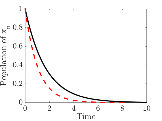
We consider the system in Fig. 1 with mutants, replication rate , and control penalty . A nominally optimal drug dose was designed to minimize for the nominal model (i.e., ) and a robust optimal drug dose was designed to solve the robust optimal control problem considered in Theorem 5 with the assumption (i.e., and all other , or, equivalently, ). The designed doses were,
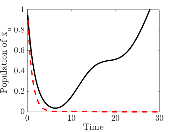
Any destabilizes a system controlled by and any destabilizes a system controlled by .
Figure 2(a) shows the impulse response for the nominal model controlled by and . Figure 2(b) shows the closed loop impulse response when . The nominal controller is more sensitive to perturbations in the model.
6 Concluding remarks
We study an infinite horizon optimal control problem for a class of monotone bilinear systems. The objective function is given by the induced power norm which represents a generalization of the performance metric. We prove that the optimal control signal is constant over time, show that the optimal controller can be computed by solving a finite-dimensional non-smooth convex optimization problem, and develop a subgradient algorithm to compute the optimal solution. We further extend our results for systems with uncertain dynamics and show that computing the optimal robust controller is no harder than computing the nominal controller. Finally, we apply our results to an example inspired by combination drug therapy design for the treatment of HIV.
Acknowledgments
The authors would like to acknowledge Peyman Mohajerin Esfahani and Kevin Nowland for helpful discussions on functional analysis.
References
- [1] E. Hernandez-Vargas, P. Colaneri, R. Middleton, F. Blanchini, Discrete-time control for switched positive systems with application to mitigating viral escape, ” Int. J. Robust Nonlin. 21 (10) (2011) 1093–1111.
- [2] E. A. Hernandez-Vargas, P. Colaneri, R. H. Middleton, Optimal therapy scheduling for a simplified HIV infection model, Automatica 49 (9) (2013) 2874–2880.
- [3] P. Colaneri, R. H. Middleton, Z. Chen, D. Caporale, F. Blanchini, Convexity of the cost functional in an optimal control problem for a class of positive switched systems, Automatica 4 (50) (2014) 1227–1234.
- [4] A. Rantzer, B. Bernhardsson, Control of convex monotone systems, in: Proceedings of the 53rd IEEE Conference on Decision and Control, 2014, pp. 2378–2383.
- [5] V. Jonsson, A. Rantzer, R. M. Murray, A scalable formulation for engineering combination therapies for evolutionary dynamics of disease, in: Proceedings of the 2014 American Control Conference, 2014, pp. 2771–2778.
- [6] V. Jonsson, N. Matni, R. M. Murray, Reverse engineering combination therapies for evolutionary dynamics of disease: An approach, in: Proceedings of the 52nd IEEE Conference on Decision and Control, 2013, pp. 2060–2065.
- [7] V. Jonsson, N. Matni, R. M. Murray, Synthesizing combination therapies for evolutionary dynamics of disease for nonlinear pharmacodynamics, in: Proceedings of the 53rd Conference on Decision and Control, IEEE, 2014, pp. 2352–2358.
- [8] N. K. Dhingra, M. R. Jovanović, Convex synthesis of symmetric modifications to linear systems, in: Proceedings of the 2015 American Control Conference, Chicago, IL, 2015, pp. 3583–3588.
- [9] N. K. Dhingra, M. Colombino, M. R. Jovanović, On the convexity of a class of structured optimal control problems for positive systems, in: Proceedings of the 2016 European Control Conference, Aalborg, Denmark, 2016, pp. 825–830.
- [10] L. Farina, S. Rinaldi, Positive Linear Systems: Theory and Applications, John Wiley & Sons, 2011.
- [11] A. Rantzer, Scalable control of positive systems, Eur. J. Control 24 (2015) 72–80.
- [12] A. Rantzer, On the Kalman-Yakubovich-Popov lemma for positive systems, IEEE Trans. Automat. Control 61 (5) (2016) 1346–1349.
- [13] N. K. Dhingra, M. Colombino, M. R. Jovanović, Leader selection in directed networks, in: Proceedings of the 55th IEEE Conference on Decision and Control, Las Vegas, NV, 2016, to appear.
- [14] M. Colombino, R. Smith, Convex characterization of robust stability analysis and control synthesis for positive linear systems, in: Proceedings of the 53rd IEEE Conference on Decision and Control, Los Angeles, California, 2014, pp. 4379–4384.
- [15] M. Colombino, R. Smith, A convex characterization of robust stability for positive and positively dominated linear systems, IEEE Trans. Automat. Control 61 (7) (2016) 1965–1971.
- [16] A. S. Besicovitch, Almost Periodic Functions, Dover Publications, 1954.
- [17] C. Corduneanu, Almost periodic oscillations and waves, Springer Science & Business Media, 2009.
- [18] C. Constanda, M. E. Perez, Integral methods in science and engineering, Springer, 2010.
- [19] J. Mari, A counterexample in power signals space, IEEE Trans. Automat. Control 41 (1) (1996) 115–116.
- [20] T. Tanaka, C. Langbort, The bounded real lemma for internally positive systems and H-infinity structured static state feedback, IEEE Trans. Automat. Control 56 (9) (2011) 2218–2223.
- [21] S. Boyd, L. Vandenberghe, Convex optimization, Cambridge university press, 2004.
- [22] P. Kokotović, H. K. Khalil, J. O’Reilly, Singular perturbation methods in control: analysis and design, SIAM, 1999.
- [23] H. K. Khalil, Nonlinear Systems, 3rd Edition, Prentice Hall, 1996.
- [24] D. P. Bertsekas, Nonlinear programming, Athena Scientific, 1999.
- [25] S. Boyd, L. Vandenberghe, Convex optimization, Cambridge University Press, 2004.
- [26] N. Z. Shor, Minimization methods for non-differentiable functions, Vol. 3, Springer Science & Business Media, 2012.
- [27] A. Beck, M. Teboulle, A fast iterative shrinkage-thresholding algorithm for linear inverse problems, SIAM J. Imaging Sci. 2 (1) (2009) 183–202.
- [28] N. Parikh, S. Boyd, Proximal algorithms, Foundations and Trends in Optimization 1 (3) (2013) 123–231.
- [29] R. A. Horn, C. R. Johnson, Matrix analysis, Cambridge university press, 1985.
- [30] M. Colombino, A. B. Hempel, R. S. Smith, Robust stability of a class of interconnected nonlinear positive systems, in: Proceedings of the 2015 American Control Conference, Chicago, IL, 2015, pp. 5312–5317.