A generalization of Marstrand’s theorem and a geometric application
Abstract
In this paper we prove two general results related to Marstrand’s projection theorem in a quite general formulation over metric spaces under a suitable transversality hypothesis (the “projections” are in principle only continuous) - the result is flexible enough to, in particular, recover most of the classical Marstrand-like theorems. Our proofs use more elementary tools than many classical works in the subject. Also we show a geometric application of our results.
1 Introduction
Let be a subset of complete metric space, a probability space and a continuous functions. Informally, one can think of as a family of projections parameterized by . We assume that for some positives real numbers the following transversality property is satisfies:
| (1.1) |
for all and all .
We proof a general versions of Marstrand theorem assuming that is an analytic subset of a complete metric space. Thus,
Theorem 1.1.
Let be an analytic subset of a complete metric space.
-
1.
Suppose , then for almost every .
-
2.
Suppose that , then for almost every .
2 Preliminaries
Let be a metric space, for and we will denote by the ball of center and radius .
If is a subset of , the diameter of is and, if is a family of subsets of , the diameter of is defined as
Given and denote , define the Hausdorff -measure as
It is not difficult to show that there exists a unique for which if and if . We define the Hausdorff dimension of as .
It is important to emphasize a Howroyd’s result about finite Hausdorff dimension (see [How95]).
Lemma 2.1 (Howroyd).
Every analytic subset of a complete metric space which positive (or infinite) Hausdorff -measure contains a compact set, which has finite and positive Hausdorff -measure.
3 Proof of the Theorems
When is analytic subset of complete metric space and , the Lemma 2.1 stated that (see [How95]) there is a compact subset of and such that .
Thus, from now on, we can assume is compact and satisfies for some .
The following result, is analogue to Frostman Lemma.
Lemma 3.1.
There exists compact such that and there is a constant such that
| (3.1) |
for all and all .
Remark: We may have (perhaps increasing the value of ) arbitrarily small.
Proof.
By definition of Hausdorff dimension, there is such that .
Consider the constant and put . Then, suppose for some and some , we call the collection of balls for , that satisfies the above property.
Claim: The set satisfies
| (3.2) |
Proof of Claim: Taken a disjoint collection of elements of such that . Assume, without loss of generality, that sequence is decreasing.
We stated that . In fact:
Let and consider . If we have noting to do. Therefore, suppose that . If for all , , then by definition of should be and this is a contradiction with definition of . Thus, there is such that and . This last condition provides us that as we wishes.
However, by definition of , for all ratio of some ball in . Therefore,
| (3.3) |
since , then we concluded the proof of claim.
Now consider the set that satisfies
Moreover, by definition of we have that for . Also, for we have that , then
| (3.4) |
Thus, taking we finished the proof. ∎
Assume now that satisfies , for all and all .
Lemma 3.2.
There is such that for all there is a covering of by balls , with for all with the following properties
-
1.
.
-
2.
For all and , we have .
Proof.
There is such that . Let .
As is compact, then we start with a finite covering of with , .
For , let . The sets are disjoint and cover . We take, for each , a covering of by balls (which effectively intersect ) with and .
The balls form a covering of from which we extract a finite subcovering (whose elements we denote provisionally by - we will abuse of this notation; we will modify this covering but we will keep this notation). If, for some and some , there are balls from this subcovering contained in for which , we replace all these balls by . Doing this, the total number of balls in the covering and the sum of the -th power of their radii decrease, and we obtain a new covering (whose elements we still denote by ). Now, and until it is possible, we do the same procedure, which reduces the number of balls in the covering. After a finite number of steps, we arrive at a finite covering of by balls , with for all such that, for every and every , the sum of the -th power of the radii of the balls of the covering contained in never exceeds . By construction, we may associate to each such ball a nonempty finite collection (perhaps with one element) of balls of the type contained on it (perhaps itself is of this form, otherwise we take the collection of balls of this form originally deleted in the process of creation of ) with . Each ball of the type belongs to at most one of these collections. Notice that, since , we have .
Now, given and , if a ball from the above covering is contained in , for each ball from the collection associated to , we have , and thus, since and , we have . Therefore, since is at most the sum for the balls of its associated collection of , and each ball of the type belongs to at most one of these collections, the sum for all such values of is at most
with , since for all .
Finally, we have
∎
Proof of Theorem 1.1.
Let’s prove the first part of the theorem, and we will use the first part to prove the second part of the theorem.
Take small. Since is a compact set, we can consider a covering of by balls , with for all as in Lemma 3.2. We define the following family of functions :
It is to easy see that , where is a -neighborhood of .
The idea now is to show that , so we have that almost every .
In fact:
The first part of the right side of the above inequality is bounded. Let’s calculate the integral on for the second part of the right side of the above inequality.
We use the notation , thus, as the sequence of ’s are decreasing, then
Note that the transversality condition (1.1) we have that
Therefore,
| (3.5) | |||||
The next step is to estimate the sum of the right side of the previous inequality, for this assume that and remember that , then
Thus, we can conclude that .
Given , . Thus, taking , there are such that and for we have , which implies that , then for infinitely many values of . Here
By the Cauchy-Schwarz inequality we have
However, the first condition of Lemma 3.2 gives us
therefore we get that if , then for infinitely many indexes , which implies that . Finally, taking , we have that
and for any .
This finishes the proof of first part of theorem.
Let’s proof the second part of theorem, using the first part.
We consider two cases:
-
Case 1:
. Assume that (for general case see Remark 3.3). Then given small, we consider the two regular Cantor sets such that
(3.6) Consider the conjugation map between and . The equation (3.8) implies that map is -Holder. Moreover, there is such that
(3.7) However, we define a new projection by . Here is the closed ball of center and radius .
-
Case 2:
. Assume that (for general case see Remark 3.4). Then given small, we consider the two regular Cantor sets such that
(3.8) Consider the conjugation map between and . The equation (3.8) implies that map is -Holder. Moreover, (abusing of notation, using the same constant as case 1) there is such that
(3.9) However, we define a new projection by .
Then we can state that, in the case 1 or the case 2, the projection is transverse. In fact: Consider the metric in , given by . Fix the points and put , without loss o generality, we call . We consider two possibilities:
-
i.)
.
Consider a point such that , then for all we have thatSo, let be the Lebesgue measure of , then and therefore
and the transverse condition is satisfied.
-
ii.)
.
Taken such that .
If , then for and such that , then which impliesThe transverse condition of provides that if , then
If , then for such that
(3.10) hold that
This last inequality implies that, if we want transversality of , then we consider values of does not satisfies the equation (3.10). However, since is transverse, then
(3.11) Moreover, assume that for some , then if (note that )
Thus, we can conclude that
Taking we concluded that the transverse condition is satisfied.
So, in any case i) or ii) we have the transverse condition.
For conclude the proof of second part of theorem, note that in both cases and , the projection is transverse.
-
1)
For the case : Since , then by the first part of theorem hold that for almost every . Therefore,
as is arbitrary we conclude that for almost every , as we wished.
-
2)
For the case : Since , then by the first part of theorem hold that for almost every . Thus, , which implies that
as is arbitrary and , we conclude that for almost every , as we wished.
∎
Remark 3.3.
The proof for the general case 1 is by induction. Assume that If , then . Therefore, we consider two regular Cantor sets such that
Consider the conjugation map between and , then the function is -Holder. Moreover, there is such that
However, we define a new projection
by .
Analogously, as the previous proof, the the projection is transverse and
the conclusion follows by induction.
Remark 3.4.
The proof for the general case 2 is also by induction. Assume that If . We consider two regular Cantor sets such that
Consider the conjugation map between and . Moreover, the function is -Holder.
However, we define the projection
by .
Analogously, as the previous proof, the the projection is transverse and
the conclusion follows by induction.
4 An Example: A version of Marstrand’s theorem in non-positive curvature
4.1 Setting
We will denote a Hadamard manifold, i.e., a Riemannian manifold with metric , simply connected and of non-positive curvature. A line in is a geodesic defined for all parameter values and minimizing distance between any of its points, that is, is an isometry. If dim, then the space of lines leaving a point can be seen as a sphere of dimension . So, for surfaces the set of lines leaving a point can be identified with in the space tangent of the point . Therefore, in each point on the surface the set of lines can be oriented and parametrized by and endowed with the Lebesgue measure. Thus, using the previous identification, we can talk about almost every line through a point of (cf. [BH99]).
The law of cosines state that
where is the angle in between the segments of geodesic and .
Gauss’s Lemma: Let and let and . Then,
Let be a complete convex set in . The orthogonal projection (or simply ‘projection’) is the name given to the map constructed in the following proposition: (cf. [BH99, pp 176]).
Proposition 4.1.
The projection satisfies the following properties:
-
1.
For any there is a unique point such that .
-
2.
If is in the geodesic segment , then .
-
3.
Given , and , then .
4.2 Geometric Marstrand
Let’s use the theorem 1.1 for prove the the following theorem:
Theorem 4.2 ( Geometric Marstrand ).
Let be a Hadamard surface, analytic and be given. Then
-
1.
If then, for almost every line coming from p, we have that has positive Lebesgue measure, where is the orthogonal projection on .
-
2.
If then, for almost every line coming from p, we have that , where is the orthogonal projection on .
The Hadamard’s theorem (cf. [dC08]), stated the a Hadamard manifold is diffeomorphic to . Therefore, from now on, we can assume, for dimension , that .
Fix and let be a positive orthogonal basis of , i.e., the basis has the induced orientation of . In this coordinates, we call . Denote by the line through with velocity , given by , denote by the projection on .
Then, given , we can define by the unique parameter such that i.e., and
However, the previous theorem can be state as follows:
Theorem 4.3.
Let be endowed with a metric of non-positive curvature, and analytic. Then:
-
1.
If then, for almost every , we have that , where is the Lebesgue measure.
-
2.
If then, for almost every , we have that , where is the orthogonal projection on .
Given a line such that , then for there is a unique such that . Slightly abusing of the notation, we will write .
Fix and let be a positive orthogonal basis of , i.e., the basis has the induced orientation of . Then, call in coordinates the unit vector . Denote by the line through with velocity , given by and by the projection on .
Then, given , we can define by the unique parameter such that i.e., and
Remark 4.4.
Given , consider the unique geodesic such that and , then there are unique , such that the geodesic intersect orthogonality the geodesic in the point
and the basis is positive. Note that is defined even if passes through .
For denote by the angle such that the geodesic passes through in positive time.
Lemma 4.5.
Let a compact set, then for any with the function is differentiable close to . Moreover, there is a constant such that for all .
We will use this Lemma to prove Theorem 4.3.
4.3 Proof of Lemma 4.5
Before to prove the lemma 4.5 we will give some definitions and prove some auxiliaries lemmas.
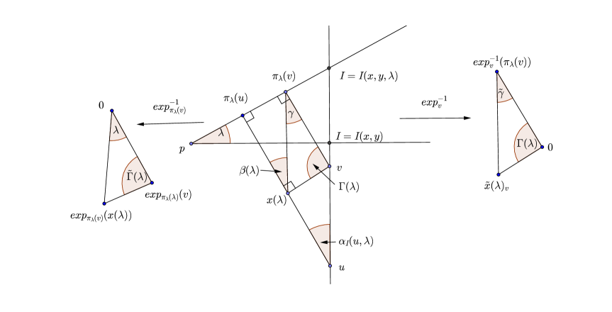
Given , if the geodesic does not pass through , then for small we can define the function
for all . We denote by the unique point of intersection of the geodesic with the geodesic (cf. Figures 1(a), 1(b)). On the other hand, if the geodesic passes through (cf. figure 2), then for small and we define the function
Lemma 4.6.
The functions are differentiable. Moreover, the function is differentiable in .
Proof.
The differentiability of and is an immediate consequent of the convexity of the distance function and Theorem of Implicit Functions.
For prove the second part, suppose that pass through , then is constant equal to , which is differentiable. Therefore, we can assume that does not pass through , then there is a neighbourhood of such that is a Poincaré-like map between and defined as the intersection of the geodesic with for . Therefore, there is small such that
. Thus we concluded the proof of second part.
∎
Lemma 4.7.
For , we have
-
1.
If the geodesic does not passes through , then the functions and are differentiable in . Moreover,
-
2.
If the geodesic passes through , then the functions and are differentiable in . Moreover,
Proof.
The differentiability of both functions follows of Lemma 4.6 and the differentiability of exponential map.
For the Limit we consider two cases:
-
Case 1:
Suppose that the geodesic does not pass through (cf. Figure 1).
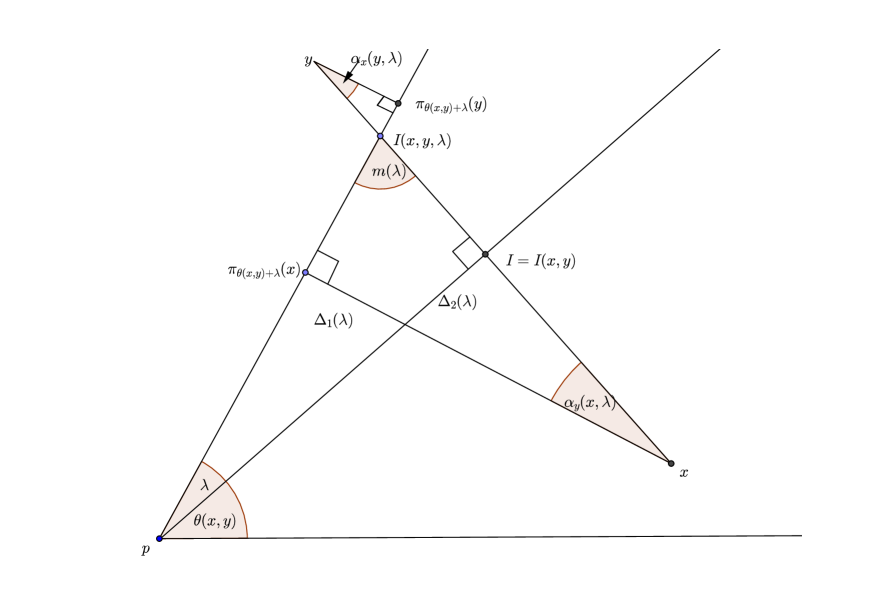
(a) 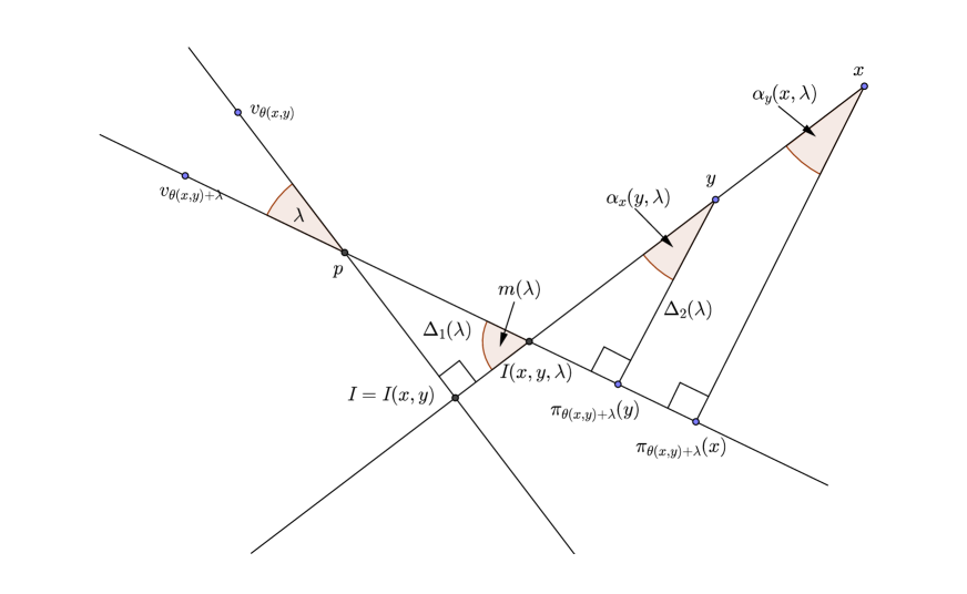
(b) Figure 1: does not pass through of Put and consider the triangle generated by the points and let for , so, by lemma 4.6, since is differentiable in , the function is differentiable in . Then, by the Gauss-Bonnet theorem the function
where denotes the Gaussian curvature, satisfies
which is also differentiable. Moreover, since then has a maximum in , thus . So, we have that .
Analogously, considering the triangle generated by the points , we have that the function is differentiable with maximum in . Thus , which implies thatTherefore, . The proof for is analogous.
-
Case 2:
Let’s assume now that the geodesic passes through (cf. Figure 2).
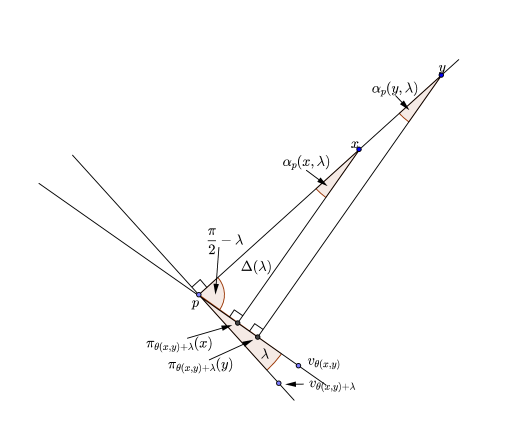
Figure 2: passes through of
In this case, consider the triangle generated by the points . Analo-
gously as above, the function
is differentiable, with maximum in , then .
The proof for is analogous.
∎
Corollary 4.8.
There is such that for all , and all we have
-
1.
If the geodesic does not pass through , then
-
2.
If the geodesic passes through , then
Lemma 4.9.
Given three different points then
Proof.
By the law of cosines
∎
Given three different points . Put , , and . Then we have the following
Lemma 4.10.
Proof.
Consider the triangle in generates by the points and the triangle in generates by the points . The by law of sines
The conclusion follows by Remark 4.4. ∎
Lemma 4.11.
Given three different points with , then there is such that
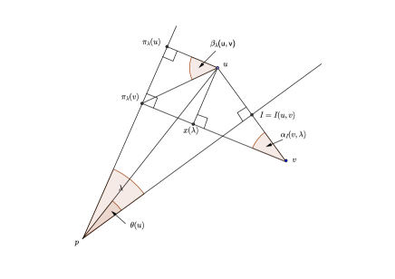
Proof.
Call the geodesic orthogonal to in . Let be such that and put and the vector that forms a angle with . The function is defined as the unique point where the geodesic meet the geodesic . Thus, there exists a unique such that . It is easy to see that, follow the same arguments of the proof of second part of lemma 4.6, the function is differentiable in . Consider the function which is also differentiable. If denotes the angle between and . The definition of and implies that
Therefore, the Gauss Lemma provides that . Thus, we can conclude that then
Thus, since , the above equation implies that there are and independent of such that
Since , the definition of implies that there is a constant such that . Therefore, by the law of sines, if ,
Taking . As we concluded the proof.
∎
Remark 4.12.
Observe that the previous Lemma holds if for some , because we only need that for some .
Proof of Lemma LABEL:L1.
Without loss of generality we can assume that .
Since , the differentiability of follows of lemma 4.6.
Now, for prove the second part of lemma, we can assume first that the geodesic does not pass through of point . Denote and . Let us subdivide the proof in two cases:
-
1)
,
-
2)
.
Let us first prove the case 1 (cf. Figure 3). In fact, by lemma 4.9,
Let be given by Corollary 4.8. Then, for , we have
| (4.3) | |||||
For the second case (, cf. figure 4), without loss of generality we can assume that for small it holds that . Denote , the projection of over the geodesic segment . Then, by lemma 4.9,
where .
Considering the triangle in given by the points , and
, then, by the law of sines, , where and .
Since we have that
Using lemma 4.9 and Corollary 4.8 we have that
Now, since , remark 4.4 and Gauss Bonnet Theorem imply that as . Thus, we can assume that there is a constant such that
| (4.4) |
Considering the triangle in given by the points , and , if then, by the lemma 4.10 implies that
where . Thus, since as , the remark 4.12 of lemma 4.11 implies that there is a constant such that for , which provides that
| (4.5) |
Moreover, as the curvature is non-positive, then , thus, as the sine is a increasing function and , then without loss of generality, we have for . This last inequality together with the equations (4.4) and (4.5) implies that
| (4.6) |
Taking , we conclude that
Therefore, the equations (4.3) and (4.6) implies, that in any case, as we wished.
For finish the proof of lemma, we note that if the geodesic does not pass through of , then we can make the proof similar to the second case above.
∎
References
- [BH99] M. R. Bridson and A. Haefliger. Metric spaces of non positive curvature. Grundlehren der Matematischen Wissenchaften, vol. 319 - Springer-Verlag, Berlin, 1999.
- [dC08] M. P. do Carmo. Geometria Riemaniana. Projeto Euclides, IMPA, 4th edition, 2008.
- [How95] J.D. Howroyd. On dimension and on the existence of sets of finite positive Hausdorff measure. Proc. London Math. Soc. (3), 70:581–604, 1995.
- [Sol97] Boris Solomyak. On the measure of arithmetic sums of cantor sets. Indagationes Mathematicae, 8(1):133–141, 1997.
IMPA-Estrada D. Castorina, 110-22460-320- Rio de Janeiro-RJ-Brazil
E-mail address: gugu@impa.br
IMPA-Estrada D. Castorina, 110-22460-320- Rio de Janeiro-RJ-Brazil
E-mail address: waliston@yahoo.com
IM-Universidade Federal do Rio de Janeiro-
Av. Pedro Calmon, 550 - Cidade Universitária, 21941-901, Rio de Janeiro-RJ-Brazil,
E-mail address: sergiori@im.ufrj.br