Semantic Facial Expression Editing using Autoencoded Flow

Abstract

High-level manipulation of facial expressions in images — such as changing a smile to a neutral expression — is challenging because facial expression changes are highly non-linear, and vary depending on the appearance of the face. We present a fully automatic approach to editing faces that combines the advantages of flow-based face manipulation with the more recent generative capabilities of Variational Autoencoders (VAEs). During training, our model learns to encode the flow from one expression to another over a low-dimensional latent space. At test time, expression editing can be done simply using latent vector arithmetic. We evaluate our methods on two applications: 1) single-image facial expression editing, and 2) facial expression interpolation between two images. We demonstrate that our method generates images of higher perceptual quality than previous VAE and flow-based methods.

1 Introduction

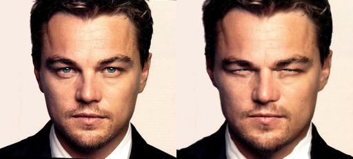
Figure 1: Illustration of the facial expression manipulation task. Left: Source image.Right: Squint expression synthesized automatically by our method.

The pixel-level manipulation of photographs is a common task that has received considerable attention, both in the form of commercial products and research papers. High-level, semantic editing of images, such as turning a frown into a smile, is much less well-understood, because it requires holistic understanding of how images correspond to linguistic concepts. Recent and dramatic advances in image understanding, however, suggest that we can start performing these types of semantic image edits.

In this paper we address the problem of high-level facial expression editing, such as changing emotions. For example, we take a neutral face photo and make it smile, or squint, or exhibit disgust. We can also exaggerate an existing expression, or perform the opposite task of making an expression subtler. Finally, we also show how to interpolate between two facial expressions, while maintaining a more realistic image than a simple cross-fade or morph would afford.

Our approach to realistic facial expression manipulation is inspired by recent facial synthesis work using convolutional neural networks (CNNs) [14, 27, 7]. These techniques model the space of realistic faces by auto-encoding a dataset of faces down to a low-dimensional latent vector; they then generate a face image from this latent vector. The advantage of this latent space is that it is more linear than the space of general images [22, 14]. When this space is well-formed, sampling novel latent vectors yields novel but realistic face images. Also, interpolating latent vectors yield realistic interpolated faces, and certain directions in the latent space are aligned with semantic properties, such as smiles, or beards.

These methods show impressive and exciting generalization capabilities, and can generate recognizable faces over a wide range of identities and expressions. However, close inspections of these generated images often reveal low resolution, blurriness, and broken facial features. Not surprisingly, synthesizing faces by hallucinating RGB values from scratch is very difficult. An alternative and less ambitious approach, long employed by the graphics community [19, 2], is to generate or manipulate images by re-using parts of existing ones. While these results are often high-resolution and very realistic, the lack of a latent space prevents more high-level, semantic operations.

In this paper we explore whether the strengths of these two methods can be combined. Inspired by recent techniques that place differentiable optical flow layers within neural networks [10, 32], we train an autoencoder that learns to synthesize face images by flowing the pixels of existing face images. Instead of a latent space that directly encodes RGB values of face images, our latent space encodes how to flow one face image to another of the same person. We show that this approach allows us to maintain the high-resolution, sharp textures of existing images while manipulating images in a meaningful latent space.

2 Related Work

Deep neural network methods for image synthesis have recently produced impressive results [14, 27, 7, 5, 21, 20]. Many of these techniques employ an additional adversarial network to further optimize the appearance of the generated image [5, 21]. The most similar paper to our work is DeepWarp [6], which also uses neural networks to synthesize flow fields that manipulate facial expression. However, this technique is specifically limited to changing the gaze direction of eyes in an image, most typically for video-conferencing applications.

Traditional graphics techniques for editing and synthesizing facial expressions operate by manipulating patches of existing images. The Visio-lization method [19] hallucinates novel faces by compositing facial patches from a large dataset. Optical flow computed over 3D face models allow facial expression manipulation and compositing of expressions [28, 29, 30]. Beyond faces, feature correspondence has long been used to warp and morph images [3]. We compare the results of our CNN-based method against both morphing and optical flow in Section 6.

3 Approach

Deep generative models, such as Variational Autoencoders (VAEs) [13], have demonstrated that image generation and editing can be done through vector arithmetic in the latent space [27, 21, 14]. Inspired by those models, we proposed the Flow Variational Autoencoder (FVAE) model, which is a hybrid of VAE and the classical flow-based approach [30, 28]. In particular, the decoder of our FVAE learns a mapping from the latent space to the flow space, rather than pixel space.

The FVAE takes a pair of source and target images as input and outputs a per-pixel flow field and a per-pixel confidence mask. The flow field warps the source image to be similar to the target image, and the confidence mask indicates how confident the model is with its flow predictions.

In the following sections, we describe our objective functions to train a FVAE, and how to utilize a trained FVAE for two applications: 1) single image facial expression editing and 2) facial expression interpolation between two face images.

3.1 Learning Flow Variational Autoencoder

The objective function for learning a FVAE consists of three parts: 1) $\mathcal{L}_{reconstruct}$, which controls the pixel-wise image difference, 2) $\mathcal{L}_{prior}$, which controls the smoothness in the latent space, and 3) $\mathcal{L}_{flow}$, which controls the coherence in the flow space. The overall objective is to minimize the following loss function,

$$\mathcal{L}=\mathcal{L}_{reconstruct}+\lambda_{1}\mathcal{L}_{prior}+\lambda_{2}\mathcal{L}_{flow}$$ (1)

where $\lambda_{1}$ and $\lambda_{2}$ are hyperparameters to be tuned.

3.1.1 FVAE Variational Autoencoder

We first denote the following notations that will be used throughout the formulation: $T$ = target image, $S$ = source image, $f$ = encoder, $g$ = decoder, $D$ = set of $(S,T)$ tuples in the dataset, and $Z$ = latent vector.
Encoder Network $f(T)$: Following the VAE framework [13], we assume the prior distribution follows a multivariate Gaussian distribution. Using the reparameterization trick, our model’s encoder network, $f(T)=(\boldsymbol{\mu}(T),\boldsymbol{\sigma}(T))$, outputs the mean $\boldsymbol{\mu}$, and standard deviation $\boldsymbol{\sigma}$ of the approximate posterior. To compute the latent vector $Z$ for a given $T$, we sample a random $\epsilon$ from the multivariate Gaussian distribution, $\mathcal{N}$.

$$Z(T)=\boldsymbol{\mu}(T)+\boldsymbol{\sigma}(T)\odot\boldsymbol{\epsilon}$$ (2)

where, $\boldsymbol{\epsilon}\sim\mathcal{N}(0,\mathbf{I})$.
As proposed and derived in [13], $\mathcal{L}_{prior}$ has the following form,

$$\mathcal{L}_{prior}=-\sum_{T\in D}\sum_{k}\bigg{(}1+\log(\sigma_{k}^{2}(T))-\mu_{k}^{2}(T)-(\sigma_{k}^{2}(T))\bigg{)},$$ (3)

where $k$ indexes over the dimensions of the latent space.
Decoder Network $g(S,Z(T))$: The proposed FVAE can be viewed as a constrained version of VAE, as the output of FVAE can only contain pixels flowed from the source image.

$$\mathcal{L}_{reconstruct}=\sum\limits_{(S,T)\in D}||T-g(S,Z(T))||_{2}^{2}$$ (4)

subject to $g_{j}(S,Z(T))\in\{S\}\quad\forall j$, where $j$ denotes the pixel location.

In order to satisfy the constraint the network computes a dense flow field, $F$, as an intermediate state. Denote $F(j)\triangleq(F(j)_{x},F(j)_{y})$, which specifies the pixel location to sample from $S$ to reconstruct the $j^{th}$ pixel of the output, $g_{j}(S,Z(T))$. To train the network from end-to-end, we relax the constraint in Eq.4, such that $g_{j}(S,T)$ is in the set of bilinear interpolated values from $\{S\}$  [32]. The decoder network, $g$, has the form

$$g_{j}(S,Z(T))=$$

$$\sum_{k\in N(F(j))}S_{k}(1-|F(j)_{x}-x_{k}|)(1-|F(j)_{y}-y_{k}|),$$ (5)

where $(F(j)_{x},F(j)_{y})$ denotes the absolute coordinates to sample from the source image, $N(F(j))$ denotes the set of the 4 neighbors of $F(j)$, $S_{k}$ denotes the $k^{th}$ pixel of the source image, and $(x_{k},y_{k})$ denotes the pixel absolute coordinates of the $k^{th}$ pixel.

This bilinear sampling mechanism was introduced by Jaderberg et al. as differentiable image sampling with a bilinear kernel; Error backpropagation can be done efficiently through this mechanism [10].

3.1.2 Flow Coherence Regularization

Our choice of the flow coherence regularizer, $\mathcal{L}_{flow}$, is based on the intuition that flow directions should be spatially coherent except at boundaries. We design a pair-wise regularization term as follows:

$$\mathcal{L}_{flow}=$$ (6)

$$\sum\limits_{\mathbf{i}}\sum\limits_{\mathbf{j}\in N(\mathbf{i})}||F_{\mathbf{i}}-F_{\mathbf{j}}||_{2}^{2}\exp(-(\alpha||T_{\mathbf{i}}-T_{\mathbf{j}}||_{2}^{2}+||\mathbf{i}-\mathbf{j}||_{2}^{2}))$$

where, $\mathbf{i},\mathbf{j}$ are 2D-coordinates, $F_{\mathbf{i}}$ is the flow vector at $\mathbf{i}$, $T_{\mathbf{i}}$ is a RGB color vector of the target image at $\mathbf{i}$, $\alpha$ is a weighting hyper-parameter, and $N(\mathbf{i})$ is the set of neighboring pixels of $\mathbf{i}$. In our experiment we use a $7\times 7$ neighborhood centered at $\mathbf{i}$.

Eq.6 implies that the flow is encouraged to be similar for nearby pixel coordinates, especially when RGB values are similar in the target image. Similar smoothness formulations have been used in the context of semantic image segmentation [31, 24, 4, 16].

3.2 Learning the Confidence Mask

From a single source image, it may not be possible to form a good reconstruction of the target image. For example, it will be very difficult to reconstruct a smile expression given a neutral expression, as the teeth region simply does not exist in the source image. Ideally, we would like to have a mechanism to identify the regions where the network will perform poorly given a particular pair of source and target image. With such a mechanism, we would be able combine multiple source images to generate one output image.

In order to identify such regions, we trained another network to predict a per-pixel soft confidence mask $M$ where $M_{j}$ predicts the confidence of the generated output $g_{j}(S,Z(T))$. This confidence-learning problem can be formulated as a binary classification task, where the label is 1 if the target pixel is in the source image, and 0 otherwise. However, getting such labels would require searching each pixel pair in $S$ and $T$ for all $(S,T)$ pairs, and is not scalable. Instead we choose to approximate the true label, $y$, using the $\ell_{2}$-norm, as follows:

Given a trained encoder $f$ and decoder $g$,

$$y=\exp\bigg{(}-\frac{||T-g(S,Z(T))||_{2}^{2}}{\beta}\bigg{)}$$ (7)

, where $\beta$ is a normalization constant, such that $y\in[0,1]$.

The confidence mask network takes $Z(T)$ and $S$ as inputs (i.e., $M(S,Z(T))$), as at test-time the target image is not available. With the approximate true label $y$, the objective function for learning the confidence mask is the sum of cross entropy losses over all pixel locations. To train the network we minimize the following loss function:

$$\mathcal{L}_{mask}=-\sum\limits_{(S,T)\in D}\sum\limits_{\mathbf{i}}y_{\mathbf{i}}\log(M_{\mathbf{i}})+(1-y_{\mathbf{i}})\log(1-M_{\mathbf{i}})$$ (8)

4 Applications

With a trained FVAE model, we proposed two applications 1) expression editing on a single source image, and 2) expression interpolation from a pair of source images.

4.1 Expression Editing Using Latent Vector

For this task, the goal is to transform the expression of a given face image to a desired target expression; see Figure 2 for illustration. The task is an analogy making problem, A:B::C:D means A is to B as C is to D [22] (i.e., generate a D such that the relationship between C and D is similar to that of A and B).

Latent representations from deep models have been shown to capture semantic and visual relationships, and analogy can be made through vector arithmetic; if A:B::C:D then $(A-B)\approx(C-D)$. For example, in language models, the vector representations of “King” - “Man” + “Woman” is a vector similar to “Queen.” [17, 18]. Similarly, visual analogy making has been explored in [22, 21].

Algorithm 1 details the method for performing expression editing using the proposed FVAE. The inputs are: 1) the trained FVAE network, $(f,g)$, 2) training dataset face images, $I$, and expression labels, $y$, 3) a source image for editing, $S$, 4) a target expression label, $y_{target}$, 5) the source expression label, $y_{source}$, and 6) the number of steps, $K$.

Algorithm 1 Expression Edit

1:Inputs:

2:      $f,g$, $D=\{(I,y)\}$, $S$, $y_{target}$, $y_{source}$, $K$

3:Initialize:

4:      $Z_{target}=\frac{1}{|D|}\sum\limits_{D}Z(I)\cdot\mathbf{1}[y=y_{target}]$

5:Initialize:

6:      $Z_{source}=\frac{1}{|D|}\sum\limits_{D}Z(I)\cdot\mathbf{1}[y=y_{source}]$

7:for each node $i=1$ to $K$ do

8:     $Z_{edit}=\frac{i\cdot(Z_{target}-Z_{source})}{K}+Z(S)$

9:     Outputs:

10:      $g(S,Z_{edit})$

11:end for

Algorithm 1 computes a latent expression direction by taking the difference of the averaged latent vectors for training images with $y_{target}$ expression label, and training images with $y_{source}$ expression label. Next, the source image’s latent vector, $Z_{source}$, is interpolated linearly along the expression direction.

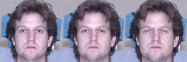
Figure 2: Traversal along the “squint direction”. The left-most image is the original image; the other two images are synthesized squint expressions at different “intensities” of squint.

4.2 Expression Interpolation Using Latent Vector

The generative power of VAE models is often demonstrated by performing linear interpolation between two given locations in the latent space. For this task, the goal is to generate all the intermediate “levels” of expression between two given source images; see Figure 6 for illustration. Algorithm 2 details the method for expression interpolation. The inputs are: 1) the two source images $S_{1}$ and $S_{2}$, 2) a trained FVAE $(f,g)$, 3) a trained mask model, $M$, and 4) the number of steps, $K$.

In order to utilize both source images in the linear interpolation, we use the normalized confidence mask to blend the interpolated outputs from each source image together. This is useful when certain facial parts are only in one of the source image, (e.g., teeth when interpolating from neutral to smile).

Algorithm 2 Expression Interpolate

1:Inputs:

2:      $f,g$, $S_{1}$, $S_{2}$, $M$, $K$

3:Initialize:

4:      $Z_{1}=Z(S_{1})$

5:Initialize:

6:      $Z_{2}=Z(S_{2})$

7:for each node $i=1$ to $K$ do

8:     $Z_{edit}=\frac{i\cdot(Z_{2}-Z_{1})}{K}+Z_{1}$

9:     $O_{1}=g(S_{1},Z_{edit})$

10:     $O_{2}=g(S_{2},Z_{edit})$

11:     $M_{1}=M(S_{1},Z_{edit})$

12:     $M_{2}=M(S_{2},Z_{edit})$

13:     Outputs:

14:      $\frac{\exp(M_{1})}{\exp(M_{1}+M_{2})}\odot O_{1}+\frac{\exp(M_{2})}{exp(M_{1}+M_{2})}\odot O_{2}$

15:end for

4.3 Flow Upsampling for High Resolution Output

Observe that one limitation of using a deep model is that the output dimensions are fixed. A model trained to generate $128\times 128$ images cannot output $512\times 512$ images. To get higher resolution output, typically, one will have to upsample in the pixel domain; this often introduces blurriness. Here we proposed to perform upsampling in the flow domain instead. We assume that high-resolution source images are available. Applying the upsampled flow to the high-resolution source images tends to produce sharper images, see Figure  7 for comparison.

5 Implementation Details

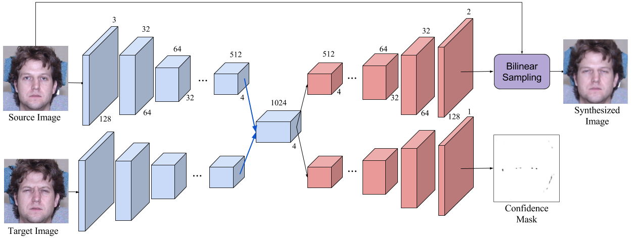
Figure 3: Detailed FVAE network architecture. The blue blocks denote convolution layers, and the red blocks denote convolution upsample layers. The blue arrows indicate concatenation. The network design follows the encoder-decoder structure in [21], where the latent space, $Z$, is the central $4\times 4\times 1024$ block.

In this section, we describe the data processing and training implementation details.

5.1 Dataset

To evaluate our proposed method, we conducted experiments on the CMU MULTI-PIE Dataset [8], which contains the identity labels to train a FVAE, as well as the expression labels necessary at test time.

5.2 Data Preparation

We use all the examples with camera view $05\_1$, and illumination $06$ from the MULTI-PIE dataset. The training and testing set is divided based on identity, with 80% and 20% random split. We aligned the faces using landmarks detected from [11], then cropped and resize the images to dimension of $128\times 128$. To prepare the training example pairs of $(S,T)$, we created all pairs of expression per identity. For each source and target image pair we apply a color transform [25] to adjust the color of the source image to better match the target images; this makes the learning easier, as $\ell_{2}$-norm loss is sensitive to lighting and color changes. We also applied data augmentation by randomly flipping images horizontally. Lastly, we normalized the pixel values into range of [-1,1] for the ease of training [21].

5.3 Model Architecture

Our model architecture follows a similar design spirit as [21]. For the encoder, convolution layers channel sizes double as the spatial size halves. For the decoder, convolution layers channel sizes halves and spatial size doubles. We used nearest neighbor interpolation for upsampling in the decoder. Figure 3, shows the exact architecture used. The convolution layers’ filter sizes are $3\times 3$, with the exception of the first and final layers, which are $5\times 5$ filters. Each convolution layer uses $relu$ except for the final layer outputting the flow which uses $tanh$, as our network outputs normalized coordinates. Additionally, all convolution layer uses batch-normalization [9], except at the final two layers before the output. All the weights are initialized from a truncated Gaussian distribution with standard deviation of 0.01.

5.4 Training

We train the network using the Adam optimizer [12], with learning rate of $0.0003$, $\beta_{1}=0.9$, $\beta_{2}=0.999$ and mini-batch size of $64$. We use gradient clipping by value with threshold of $\pm 5$. Empirically, we chose $\lambda_{1}=0.003$ and $\lambda_{2}=0.001$. The training and validation loss are monitored to use early stopping to prevent overfitting. The models are implemented using TensorFlow [1].

6 Evaluations

In this section, we provide comparison experiments with qualitative and quantitative results for the single-image editing task and image interpolation task.

6.1 Facial Expression Editing

For the facial expression editing task, we compare our FVAE model with both the VAE[13] using [21]’s architecture, and an optical flow method [23]. Figure 4 compares the expression editing results on examples from the test set. Note that for all results in our paper the person shown in the result is part of hold-out data; no images of that person were in the training set. For VAE, we train a model with the same architecture as our FVAE, except the last layer is replaced to predict the RGB pixel values directly. Then, we use Algorithm 1 to perform the editing. For optical flow, we use the average flow extracted from all identities in the training set. It can be observed that our method generates superior image quality compare to the other methods. VAE results in blurry images, and the optical flow method cannot get a flow conditioned on the source image, thus the flow is not tailored to the source image and creates artifacts.

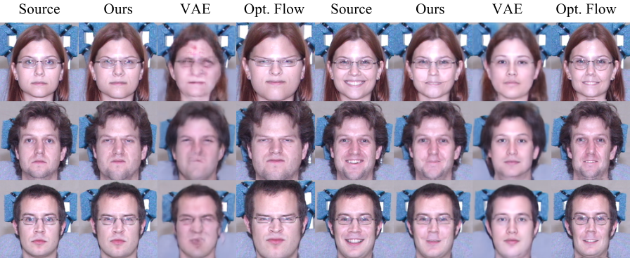
Figure 4: Comparison of synthesized expressions. Left block: Synthesis from a neutral expression source image to expression of disgust. Right block: Synthesis from a smile expression source image to a neutral expression. Our method demonstrates better low-level image quality and more realistic expressions compared to the baselines.

For quantitative evaluation, the PSNR for each method is shown in Table 1. In order to measure PSNR, we use the ground truth target image’s latent vector for FVAE and VAE. For optical flow, using a state-of-the-art method [23], we compute the flow field using the ground truth target image, and warp the source image accordingly.

It is not surprising that a VAE obtains the highest PSNR, as it is directly generating pixels to minimize the $\ell_{2}$-norm loss. However, judging by the perceptual quality, our FVAE significantly outperforms the VAE; VAE generates overly smooth images with poor low-level image quality (e.g., hair and skin textures). This just demonstrates that PSNR is not an ideal quantitative measurement for this task.

Method	PSNR
Ours	18.14
Ours w/ Confidence	18.35
VAE [13, 21]	25.41
Epic Flow [23]	15.76

Table 1: PSNR comparison between different methods. Higher is better.

Next, we demonstrate that the proposed FVAE method can be transferred to out-of-dataset samples and expressions. Figure 4 demonstrates that our method can be used to edit web images to suppress or magnify the facial expressions. The third row in Figure 4, is the expression of fear, which is not in the dataset; however, the editing can be still be done by approximating $Z_{source}=Z(S)$, in Algorithm 1. Note that for web-images to generate reasonable quality images, the background needs to be clean and the face region should not contain significant lighting variations, such as shadows.

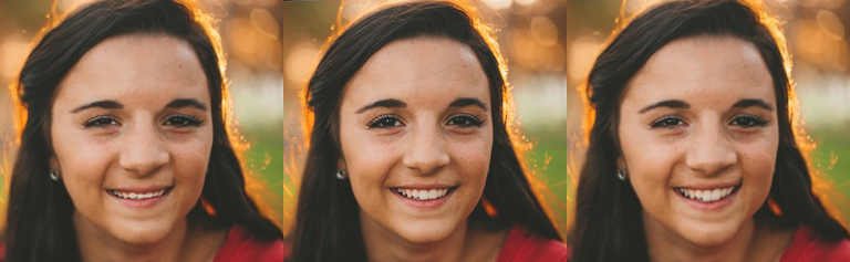
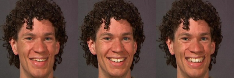
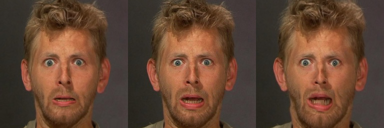
Figure 5: Magnify and suppress the facial expression. Left: Synthesized suppressed expression. Center: Original image.Right: Synthesized magnified image.

6.2 Facial Expression Interpolation

For the facial expression interpolation task, we compared our method against five different methods: VAE, cross-fading, mesh morphing [26], optical flow [15], and face morphing [29]. Figure 6 shows the qualitative comparison between the methods on examples from the test set. It can be observed that our method produces the sharpest and most realistic image out of all methods. The confidence mask successfully handles the teeth regions, whereas morphing-based methods [26, 29] and optical flow [15] generate blurry results around the mouth regions. Classical mesh morphing produces the second-best results, but still has trouble with the teeth. Moreover, our method provides a more coherent and natural transition between the expression levels.

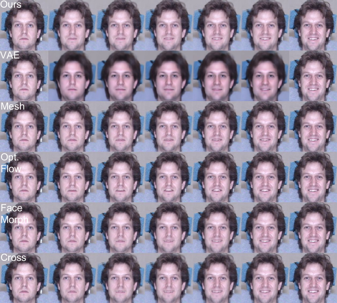
Figure 6: Image interpolation comparison. Images at both ends are the source images, and all images in between are synthesized. Row 1: Our method. Row 2: VAE. Row 3: Mesh Morphing [26]. Row 4: Optical Flow [15]. Row 5: Face Morphing [29]. Row 6: Cross Fading. Our results are perceptually better than all the baselines. The most challenging area is the mouth and teeth, because of their complicated motion and occlusions/dis-occlusions.

6.3 Perception User Study

We perform a perception user study to compare the photorealism of real images, images generated from our proposed method, VAE, and optical flow. We perform an experiment asking Amazon Mechanical Turk’s workers to label images as real or fake. The experiment is conducted on 25 participants; each is asked to label 10 examples generated from each of the methods, and 10 real images. the images are provided in random order on a single web page. To guarantee the quality of the results, users performing below 50% accuracy on the real images are dropped from the experiment. Additionally, some users skipped over certain images; we also do not count the skipped images in our result. The percentage of images labeled as real for each of the method is

reported in Table 2. As can be seen, our method outperforms VAE and optical flow in perceptual quality.

Method	% labeled real
Real	89.7%
Ours	59.4%
VAE	35.6%
Opt. Flow	41.6%

Table 2: Photorealism comparison between different methods. Higher is better.

6.4 Effectiveness of Flow Upsampling

Figure 7 shows the comparison between upsampling in the pixel domain versus in the flow domain. The source images is of dimension $512\times 512$. In order to use our trained network of dimension $128\times 128$, we resize the source image to $128\times 128$. For comparison, we upsample the output images back to $512\times 512$ in the pixel domain. For flow based upsampling, we upsample the flow back to $512\times 512$ using bilinear interpolation. Next, we pass the upsampled flow through the bilinear sampling mechanism with the high-resolution source image to synthesize the output. As can be seen, upsampling in the pixel domain leads to blurrier results compared to the flow upsampling method. The flow upsampling method preserves more of the finer details, (e.g., edges, and facial hair texture), from the source image. We are able to upsample the flow by four times without noticeable distortions in the output image.

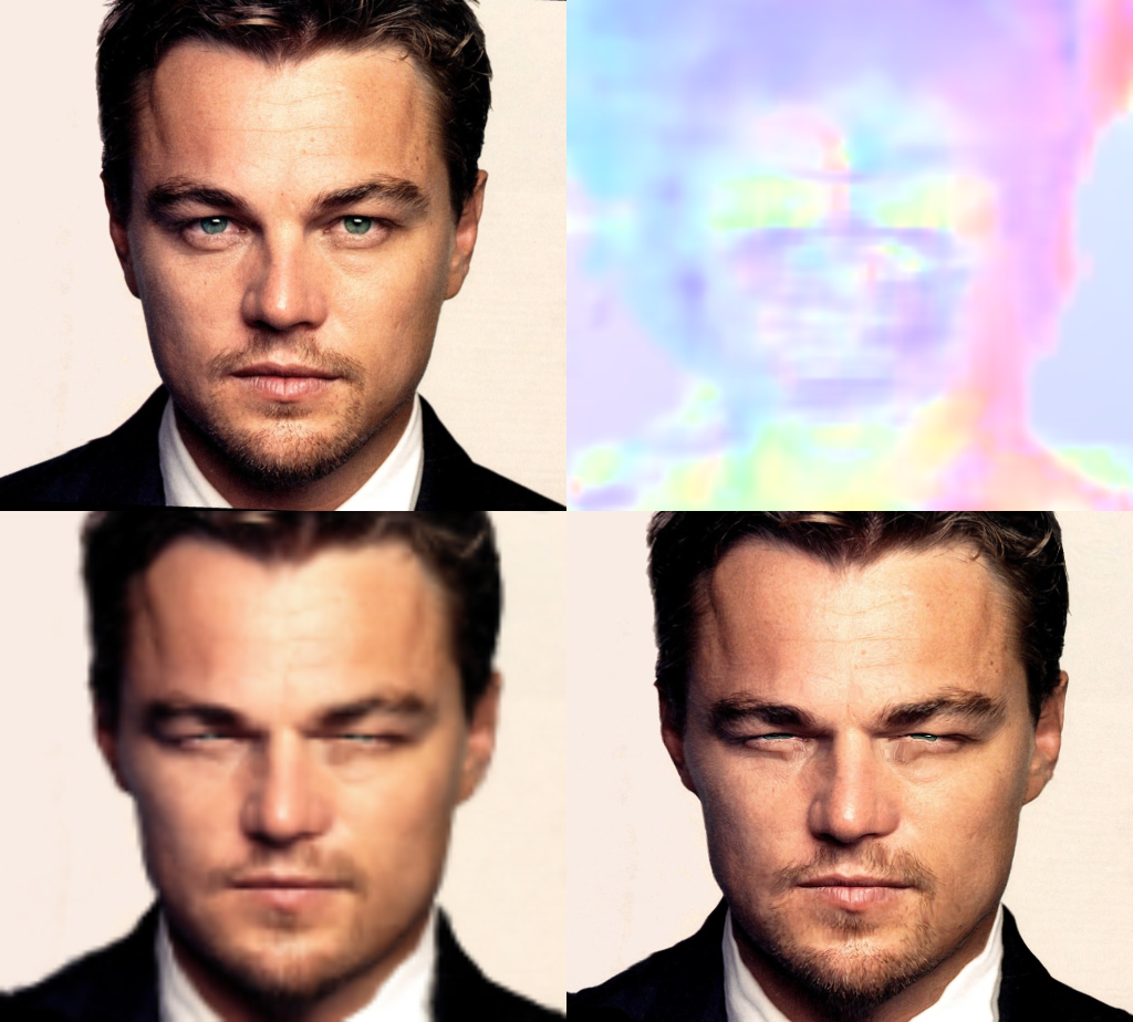
Figure 7: Upsampling comparison. Top left: High-res source image. Top right: Flow visualization. Bottom left: Pixel upsampled result. Bottom right: Flow upsample result.

7 Conclusion

We have presented an approach to the realistic manipulation of facial expressions that combines the strengths of deep models and flow-based image editing approachs. We demonstrate two applications: 1) high-level facial expression editing from a single source image, and 2) high-level facial expression interpolation from two source images. The proposed method successfully outperforms the baseline methods on the MULTI-PIE dataset. Our method generates higher resolution images, with realistic image quality and more natural expression changes. We further demonstrate that the learned transformation can be generalized to out-of-dataset samples with significantly different image statistics, while deep models hallucinating RGB values directly fail to generalize.

Despite outperforming the baseline methods, our method still faces some challenges:

1. Our method is limited to frontal pose faces with small rotations. Although  [32] demonstrates 3D rotation on objects is plausible, the task becomes more difficult when the training data does not contain a fine scales of rotated images. For example, the MULTI-PIE dataset contains 45-degree jumps between the rotation angles, and this lead to difficulties during training. However, we believe that our method can properly handle rotation given a more suitable dataset.

2. Training data needs to be very controlled. Our method requires face images taken under similar lighting conditions and backgrounds. The main reason is that $\ell_{2}$-norm loss is sensitive to RGB color changes. Without controlled data, the model will focus on learning the lighting or background difference, and less on the expression. One possible solution is to utilize face and lighting information to design a lighting and background invariant loss function.

We leave these challenges for future work.

References

- [1] M. Abadi, A. Agarwal, P. Barham, E. Brevdo, Z. Chen, C. Citro, G. S. Corrado, A. Davis, J. Dean, M. Devin, S. Ghemawat, I. Goodfellow, A. Harp, G. Irving, M. Isard, Y. Jia, R. Jozefowicz, L. Kaiser, M. Kudlur, J. Levenberg, D. Mané, R. Monga, S. Moore, D. Murray, C. Olah, M. Schuster, J. Shlens, B. Steiner, I. Sutskever, K. Talwar, P. Tucker, V. Vanhoucke, V. Vasudevan, F. Viégas, O. Vinyals, P. Warden, M. Wattenberg, M. Wicke, Y. Yu, and X. Zheng. TensorFlow: Large-scale machine learning on heterogeneous systems, 2015. Software available from tensorflow.org.
- [2] C. Barnes, E. Shechtman, A. Finkelstein, and D. B. Goldman. PatchMatch: A randomized correspondence algorithm for structural image editing. ACM Transactions on Graphics, 28(3):24:1–24:11, July 2009.
- [3] T. Beier and S. Neely. Feature-based image metamorphosis. In Computer Graphics (Proceedings of SIGGRAPH 92), pages 35–42, July 1992.
- [4] L.-C. Chen, G. Papandreou, I. Kokkinos, K. Murphy, and A. L. Yuille. Semantic image segmentation with deep convolutional nets and fully connected CRFs. Proceedings of the International Conference on Learning Representations (ICLR), 2015.
- [5] E. L. Denton, S. Chintala, A. Szlam, and R. Fergus. Deep generative image models using a Laplacian pyramid of adversarial networks. In Advances in Neural Information Processing Systems 28, pages 1486–1494. 2015.
- [6] Y. Ganin, D. Kononenko, D. Sungatullina, and V. S. Lempitsky. DeepWarp: Photorealistic image resynthesis for gaze manipulation. In Computer Vision - ECCV 2016, pages 311–326, 2016.
- [7] A. Ghodrati, X. Jia, M. Pedersoli, and T. Tuytelaars. Towards automatic image editing: Learning to see another you. CoRR, abs/1511.08446, 2015.
- [8] R. Gross, I. Matthews, J. Cohn, T. Kanade, and S. Baker. Multi-pie. Image and Vision Computing, 28(5):807–813, 2010.
- [9] S. Ioffe and C. Szegedy. Batch normalization: Accelerating deep network training by reducing internal covariate shift. In Proceedings of The 32nd International Conference on Machine Learning, pages 448–456, 2015.
- [10] M. Jaderberg, K. Simonyan, A. Zisserman, et al. Spatial transformer networks. In Advances in Neural Information Processing Systems, pages 2017–2025, 2015.
- [11] V. Kazemi and J. Sullivan. One millisecond face alignment with an ensemble of regression trees. In Proceedings of the IEEE Conference on Computer Vision and Pattern Recognition, pages 1867–1874, 2014.
- [12] D. Kingma and J. Ba. Adam: A method for stochastic optimization. In Proceedings of the International Conference on Learning Representations (ICLR), 2015.
- [13] D. P. Kingma and M. Welling. Auto-encoding variational Bayes. In Proceedings of the 2nd International Conference on Learning Representations (ICLR), number 2014, 2013.
- [14] A. B. L. Larsen, S. K. Sønderby, and O. Winther. Autoencoding beyond pixels using a learned similarity metric. In Proceedings of the 33rd International Conference on Machine Learning (ICML), 2016.
- [15] C. Liu. Beyond pixels: exploring new representations and applications for motion analysis. PhD thesis, Citeseer, 2009.
- [16] Z. Liu, X. Li, P. Luo, C. C. Loy, and X. Tang. Semantic image segmentation via deep parsing network. In Proceedings of International Conference on Computer Vision (ICCV), 2015.
- [17] T. Mikolov, I. Sutskever, K. Chen, G. S. Corrado, and J. Dean. Distributed representations of words and phrases and their compositionality. In Advances in neural information processing systems, pages 3111–3119, 2013.
- [18] T. Mikolov, W.-t. Yih, and G. Zweig. Linguistic regularities in continuous space word representations. In HLT-NAACL, volume 13, pages 746–751, 2013.
- [19] U. Mohammed, S. J. D. Prince, and J. Kautz. Visio-lization: Generating novel facial images. ACM Transactions on Graphics, 28(3):57:1–57:8, July 2009.
- [20] D. Pathak, P. Krähenbühl, J. Donahue, T. Darrell, and A. Efros. Context encoders: Feature learning by inpainting. In CVPR, 2016.
- [21] A. Radford, L. Metz, and S. Chintala. Unsupervised representation learning with deep convolutional generative adversarial networks. arXiv preprint arXiv:1511.06434, 2015.
- [22] S. E. Reed, Y. Zhang, Y. Zhang, and H. Lee. Deep visual analogy-making. In Advances in Neural Information Processing Systems, pages 1252–1260, 2015.
- [23] J. Revaud, P. Weinzaepfel, Z. Harchaoui, and C. Schmid. EpicFlow: Edge-preserving interpolation of correspondences for optical flow. In Proceedings of the IEEE Conference on Computer Vision and Pattern Recognition, pages 1164–1172, 2015.
- [24] A. G. Schwing and R. Urtasun. Fully connected deep structured networks. arXiv preprint arXiv:1503.02351, 2015.
- [25] P. Shirley. Color transfer between images. IEEE Corn, 21:34–41, 2001.
- [26] G. Wolberg. Recent advances in image morphing. In Computer Graphics International, 1996. Proceedings, pages 64–71. IEEE, 1996.
- [27] X. Yan, J. Yang, K. Sohn, and H. Lee. Attribute2Image: Conditional image generation from visual attributes. In European Conference on Computer Vision (ECCV), 2016.
- [28] F. Yang, L. Bourdev, E. Shechtman, J. Wang, and D. Metaxas. Facial expression editing in video using a temporally-smooth factorization. In Computer Vision and Pattern Recognition (CVPR), 2012 IEEE Conference on, pages 861–868. IEEE, 2012.
- [29] F. Yang, E. Shechtman, J. Wang, L. Bourdev, and D. Metaxas. Face morphing using 3D-aware appearance optimization. In Proceedings of Graphics Interface 2012, pages 93–99. Canadian Information Processing Society, 2012.
- [30] F. Yang, J. Wang, E. Shechtman, L. Bourdev, and D. Metaxas. Expression flow for 3D-aware face component transfer. In ACM Transactions on Graphics (TOG), volume 30, page 60. ACM, 2011.
- [31] S. Zheng, S. Jayasumana, B. Romera-Paredes, V. Vineet, Z. Su, D. Du, C. Huang, and P. H. Torr. Conditional random fields as recurrent neural networks. In Proceedings of the IEEE International Conference on Computer Vision, pages 1529–1537, 2015.
- [32] T. Zhou, S. Tulsiani, W. Sun, J. Malik, and A. A. Efros. View synthesis by appearance flow. arXiv preprint arXiv:1605.03557, 2016.