Bounded, efficient and multiply robust estimation of average treatment effects using instrumental variables

Abstract

Instrumental variables (IVs) are widely used for estimating causal effects in the presence of unmeasured confounding. Under the standard IV model, however, the average treatment effect (ATE) is only partially identifiable. To address this, we propose novel assumptions that allow for identification of the ATE. Our identification assumptions are clearly separated from model assumptions needed for estimation, so that researchers are not required to commit to a specific observed data model in establishing identification. We then construct multiple estimators that are consistent under three different observed data models, and multiply robust estimators that are consistent in the union of these observed data models. We pay special attention to the case of binary outcomes, for which we obtain bounded estimators of the ATE that are guaranteed to lie between -1 and 1. Our approaches are illustrated with simulations and a data analysis evaluating the causal effect of education on earnings.

Abstract

This on-line supplementary file contains proofs of propositions and theorems in the main paper, as well as additional simulation results.

Keywords: Binary outcome; Causal inference; Identification; Semiparametric inference; Unmeasured confounding

1 Introduction

Observational studies are often used to infer treatment effects in social and biomedical sciences. In these studies, the treatment assignment may be associated with various background variables that are associated with the outcome, causing the unadjusted treatment effect estimate to be biased. These background variables are often called confounders. A major challenge of causal inference in observational studies is that in practice, these confounding variables are often not fully observed, making it impossible to identify the treatment effect in view. In such settings, instrumental variable (IV) methods are useful in dealing with unmeasured confounding and have gained popularity among econometricians, statisticians and epidemiologists. Intuitively, conditional on baseline covariates, a valid IV affects the outcome through its effect on the treatment but is otherwise unrelated to the outcome.

Traditionally, the IV methods have often been used to identify and estimate the parameters indexing a system of linear structural equation models (SEMs) (Wright and Wright,, 1928; Goldberger,, 1972); see Wooldridge, (2010, §18.4.1) and Clarke and Windmeijer, (2012) for recent reviews. Under correct specification of the linear SEMs, the population average treatment effect (ATE) is equal to a certain parameter in the SEMs and can thus be consistently estimated. One such SEM can be inferred from the following system of linear regression models:

$$D =\alpha_{0}+\alpha_{1}Z+\alpha_{2}X+\alpha_{3}U+\epsilon_{D},$$ (1a)

$$Y =\beta_{0}+\beta_{1}D+\beta_{2}X+\beta_{3}U+\epsilon_{Y},$$ (1b)

where $Z$ is an instrumental variable, $D$ is a continuous treatment, $Y$ is a continuous outcome, $X$ and $U$ denote observed and unobserved baseline covariates, respectively, $Z\rotatebox[origin={c}]{90.0}{$\models$}U\mid X$ and the error terms are independent: $\epsilon_{D}\rotatebox[origin={c}]{90.0}{$\models$}\epsilon_{Y}$. In models (1a) and (1b), $\alpha_{1}\neq 0$ such that $Z$ is associated with the treatment, and the fact that conditional on $D,X$ and $U$, $Z$ is excluded from the outcome model encodes the assumption that $Z$ has no direct effect on $Y$. One can then show the parameter $\beta_{1}$ is identifiable and equals the ATE. Furthermore, it can be consistently estimated via two-stage least squares (Theil,, 1953), in which one first obtains estimates of $E[D\mid Z,X]$ through a linear regression, and then regresses $Y$ on $\hat{E}[D\mid Z,X]$ and $X$ to get the treatment effect estimate $\hat{\beta}_{1}$. However, (1a) and (1b) impose strong parametric assumptions on the underlying data generating process. Moreover, a fundamental limitation with relying on models like (1a) and (1b) is that they impose one set of assumptions, which conflates the definition, identification and estimation of the treatment effect. For example, the target parameter $\beta_{1}$ may not even be well-defined if model (1b) is misspecified.

More recently, starting with the seminal work of Imbens and Angrist, (1994), Baker and Lindeman, (1994) and Angrist et al., (1996), more attention has been drawn to using the IV model to estimate the local average treatment effect (LATE) (e.g. Abadie et al.,, 2002; Abadie,, 2003; Tan,, 2006; Cheng et al.,, 2009; Ogburn et al.,, 2015), defined as the average treatment effect for the so-called complier subgroup, partly because it is nonparametrically defined and can be identified under an assumption that the effect of the IV on the treatment is not confounded and a certain monotonicity assumption described in Section 2. In this approach, assumptions needed for identification are usually clearly separated from assumptions needed for estimation, so that a researcher is not required to commit to a specific observed data model in establishing identification. One may then construct multiple estimators that are consistent under different observed data models, or even estimators that are doubly robust in the sense that they are consistent in the union of two observed data models. However, the LATE concerns an unknown subset of the population which may be highly selective: the compliers may be more likely to believe that they would benefit from the treatment (e.g. Robins and Greenland,, 1996). Furthermore, the definition of LATE depends on the particular IV that is available (Wooldridge,, 2010, p. 605). As a result, the LATE would in general differ from the ATE, which is arguably the causal parameter of interest in most observational studies (Imbens,, 2010). We refer interested readers to Deaton, (2009), Heckman and Urzua, (2010), Pearl, (2011) and Aronow and Carnegie, (2013) for additional discussions on whether the LATE is of genuine scientific interest.

To the best of our knowledge, to date there has only been limited work focusing on ATE in the context of an IV, while successfully maintaining identification and estimation assumptions clearly separated. Prior to our work, Angrist and Fernandez-Val, (2013) and Aronow and Carnegie, (2013) assume that conditional on a covariate profile, the ATE is the same as the LATE, so that it can be identified under a monotonicity assumption, provided that the causal effect of the IV on the treatment is not confounded. Hernán and Robins, (2006) and Vansteelandt and Didelez, (2015) instead assume absence of treatment effect modification by the instrument among the treated and untreated population, respectively. In this paper, we propose two alternative no-interaction assumptions involving the unobserved confounders that allow for identification of the ATE. Our first assumption is a generalization of linear model (1a); our second assumption is similar to Hernán and Robins, (2006)’s treatment homogeneity assumption in that it is guaranteed to hold under the null of no treatment effect, but it applies to the whole population rather than the treated (or untreated) population. We also do not rely on the monotonicity assumption for identification, and allow for instruments that are confounded with the treatment. One interesting observation is that under both of our identification assumptions, the ATE can be represented by the same observed data functional so that in the estimation stage, we can target a single statistical parameter. This parameter is called the average Wald estimand, a generalization of the Wald estimand (Wald,, 1940) to accommodate baseline covariates $X$. By carefully parameterizing the efficient influence function for the average Wald estimand, we derive locally semiparametric efficient estimators that are multiply robust in the sense that they are consistent in the union of three different observed data models. This is in contrast to previous estimators for the LATE (e.g. Tan,, 2006; Ogburn et al.,, 2015), the ATE (e.g. Okui et al.,, 2012; Vansteelandt and Didelez,, 2015) and a related causal parameter, the effect of treatment on the treated (ETT) (Tchetgen Tchetgen and Vansteelandt,, 2013; Liu et al.,, 2015), wherein researchers only obtain doubly robust estimators. Furthermore, we discuss the setting of binary outcomes in detail, for which IV methods are not well developed. Towards that end, we propose variation independent parameterizations of the likelihood so that the parameter space under our model specification is unconstrained. We also propose bounded estimators for the ATE that always lie in the parameter space, which is $[-1,1]$ for a binary outcome. Throughout we assume both the instrument and the treatment to be binary.

The rest of this article is organized as follows. In Section 2, we introduce the IV set-up, provide various potential outcomes definitions we shall refer to throughout the paper and discuss existing results on partial identification. We provide formal identification conditions and corresponding estimation approaches in Sections 3 and 4, respectively. In Section 5, we evaluate the finite sample performance of the proposed estimators via simulations. In Section 6, we apply the proposed methods to estimate the causal effect of education on earnings using data from the National Longitudinal Study of Young Men. We end with a brief discussion in Section 7.

The R programs that were used to analyse the data can be obtained from https://dataverse.harvard.edu/dataset.xhtml?persistentId=doi:10.7910/DVN/BIJWCU.

2 Framework and notation

Consider an observational study with a single follow-up visit. Suppose we are interested in estimating the effect of a binary exposure $D$ on an outcome variable $Y$, but the effect of $D$ on $Y$ is subject to confounding by observed variables $X$ as well as unobserved variables $U$. A variable Z is called an IV if it satisfies the following assumptions (e.g. Didelez and Sheehan,, 2007):

• Exclusion restriction: $Z\rotatebox[origin={c}]{90.0}{$\models$}Y\mid(D,U,X)$;

• Independence: $Z\rotatebox[origin={c}]{90.0}{$\models$}U\mid X$;

• Instrumental variable relevance: $Z\not\!\perp\!\!\!\perp D\mid X.$

Figure 1 gives causal graph representations (Pearl,, 2009; Richardson and Robins,, 2013) of the (conditional) IV model.

(a). A DAG with a bi-directed arrow.

(b). A SWIG with a bi-directed arrow.

Figure 1: Causal graphs representing an instrumental variable model. The bi-directed arrow between $Z$ and $D$ indicates potential unmeasured common causes of $Z$ and $D$. Variables $X,Z,D,Y$ are observed; $U$ is unobserved. The left panel gives a causal Directed Acyclic Graph (Pearl,, 2009) with a bi-directed arrow, and the right panel gives a Single World Intervention Graph (Richardson and Robins,, 2013) with a bi-directed arrow.

An alternative definition of IV is based on the potential outcome framework (Neyman,, 1923; Rubin,, 1974), under which we assume $D(z)$, the potential exposure if the instrument would take value $z$ to be well-defined (the Stable Unit Treatment Value Assumption, Rubin,, 1980). Similarly, we assume $Y(d,z)$, the response that would be observed if a unit were exposed to $d$ and the instrument had taken value $z$ to be well-defined. The definition of IV under this framework can be derived from a single-world intervention graph (SWIG) (Richardson and Robins,, 2013) similar to the one in Figure 1(b), but without the bi-directed arrow $Z\leftrightarrow D(z)$. In particular, A1 is replaced with the assumption A1^′ that $\forall z,Y(z,d)=Y(d)$ and A2 is replaced with the assumption A2^′ that $\forall z,d,Z\rotatebox[origin={c}]{90.0}{$\models$}(D(z),Y(d))\mid X.$ We refer interested readers to Dawid, (2003) and Richardson and Robins, (2014) for discussions on the connections and differences between these two definitions.

In this article, we assume A1^′, A2, A3 and the additional assumption A4 that $Y(d)\rotatebox[origin={c}]{90.0}{$\models$}(D,Z)\mid(X,U).$ The last assumption may also be read (via d-separation) from the SWIG in Figure 1(b). Note we allow for unmeasured common causes of $Z$ and $D$, so that the instrument $Z$ and exposure $D$ may be associated simply because they share a latent common cause. This is important as in observational settings, it may be difficult to ensure that one has measured all common causes of $Z$ and $D$. However, if $Z$ represents a randomized experiment, then one might be willing to make the stronger assumption that the causal effect of Z on D is unconfounded so that $Z\rotatebox[origin={c}]{90.0}{$\models$}D(z)\mid X$. This would allow us to remove the bi-directed arrow from the graph in Figure 1. Hernán and Robins, (2006) refer to such IVs as “causal” IVs. In this case, under the principal stratum framework (Frangakis and Rubin,, 2002), the population can be divided into four strata based on values of $(D(1),D(0))$ as in Table 1.

Table 1: Principal stratum describing potential complier status $(D(1),D(0))$

$D(1)$	$D(0)$	Principal stratum	Abbreviation
1	1	Always taker	AT
1	0	Complier	CO
0	1	Defier	DE
0	0	Never taker	NT

Under a further monotonicity assumption that $P(D(1)\geq D(0))=1,$ one is able to identify the local average treatment effect $LATE=E[Y(1)-Y(0)\mid D(1)>D(0)]$ (Imbens and Angrist,, 1994; Abadie,, 2003). However, even with a causal IV and the monotonicity assumption, the average treatment effect is not identifiable. The fundamental difficulty is that without further assumptions, it is not possible to identify the treatment effect in stratum AT or NT as the subjects in these strata always (or never) take the treatment. Instead, in the case where $Z,D,Y$ are binary and $X$ is an empty set, Richardson and Robins, (2014) derive sharp bounds for the ATE under our IV assumptions. See also Balke and Pearl, (1997) and Chesher, (2010) for sharp bounds under other definitions of IV.

3 Identification of the average treatment effect

In this section, we consider the identification problem for the average treatment effect

$$ATE=E[Y(1)-Y(0)].$$

Specifically, in the following Theorem 1, we give two general no-interaction assumptions for identification of the ATE. The proof is left to the Appendix.

Theorem 1:

Under our IV model that assumes A1^′, A2, A3 and A4, the ATE is identifiable if either of the following assumptions holds:

1. There is no additive $U-Z$ interaction in $E[D\mid Z,X,U]$:

   $$E[D\mid Z=1,X,U]-E[D\mid Z=0,X,U]=E[D\mid Z=1,X]-E[D\mid Z=0,X];$$

2. There is no additive $U-d$ interaction in $E[Y(d)\mid X,U]$:

   $$E[Y(1)-Y(0)\mid X,U]=E[Y(1)-Y(0)\mid X].$$

Furthermore, under either of these assumptions, the conditional ATE equals the conditional Wald estimand

$$ATE(x)=E[Y(1)-Y(0)\mid X=x]=\dfrac{E[Y\mid Z=1,X=x]-E[Y\mid Z=0,X=x]}{E[D\mid Z=1,X=x]-E[D\mid Z=0,X=x]}\triangleq\dfrac{\delta^{Y}(x)}{\delta^{D}(x)}\triangleq\delta(x)$$

and the marginal ATE equals the average Wald estimand $ATE=E_{X}\delta(X)\triangleq\Delta.$

Throughout for notation convenience, we say A5 holds if either A5.a or A5.b holds. A5.a is a generalization of the stage-I model (1a). It states that upon conditioning on measured covariates, no unmeasured confounder of the $D-Y$ association interacts with the IV on the additive scale in predicting the exposure. With a causal IV such that $Z\rotatebox[origin={c}]{90.0}{$\models$}D(z)\mid(X,U)$ and $Z\rotatebox[origin={c}]{90.0}{$\models$}D(z)\mid X,$ A5.a can be written in a similar form as A5.b: $E[D(1)-D(0)\mid X,U]=E[D(1)-D(0)\mid X]$. On the other hand, A5.b states that conditioning on measured covariates, no unmeasured confounder of the $D-Y$ association modifies the causal effect of $D$ on the mean of $Y$ on the additive scale. Similar to Hernán and Robins, (2006)’s treatment homogeneity assumption, A5.b has the attractive property that it is guaranteed to hold under the null hypothesis of no causal effect for all units. Assumptions A5 has an important implication for the design of observational studies: even if a randomized instrument is available, it is still important to collect as many causes of the exposure and outcome as possible in the hope that no residual effect modification remains within strata defined by covariates $X$.

It is interesting to note that with a causal IV, $\delta(X)$ may also be interpreted as $LATE(X)=E[Y(1)-Y(0)\mid D(1)=1,D(0)=0,X]$ under the monotonicity assumption that $D(1)\geq D(0),a.e.$ (Imbens and Angrist,, 1994). Hence with a causal IV, the monotonicity assumption and A5 together imply the latent ignorability assumption $LATE(X)=ATE(X)$ (Frangakis and Rubin,, 1999; Angrist and Fernandez-Val,, 2013; Aronow and Carnegie,, 2013). Similarly, under a no-current-treatment-value-interaction assumption, $\delta(X)$ can also be interpreted as $ETT(X)=E[Y(1)-Y(0)\mid D=1,X]$ (Hernán and Robins,, 2006). Consequently the no-current-treatment-value-interaction assumption and A5 together imply that $ETT(X)=ATE(X).$

However, even under the monotonicity assumption or the no-current-treatment-value-interaction assumption, our assumption does not imply that the marginal ATE is the same as the marginal LATE or the marginal ETT. The latter assumption is questionable as the complier and the treated arm may both be highly selective groups of the population. To see their differences, note that under different sets of identification assumptions described above,

$$ATE =E_{X}ATE(X)=E_{X}\dfrac{\delta^{Y}(X)}{\delta^{D}(X)};$$

$$LATE =E_{X\mid D(1)>D(0)}LATE(X)=\dfrac{E_{X}\delta^{Y}(X)}{E_{X}\delta^{D}(X)};$$ (2)

$$ETT =E_{X\mid D=1}ETT(X)=E_{X\mid D=1}\dfrac{\delta^{Y}(X)}{\delta^{D}(X)},$$

where the second equality in (2) is due to Abadie, (2003, Theorem 3.1). One can also see from (2) that with a causal IV, in the case where A5.a and A5.b are incorrect but the monotonicity assumption is correct, our estimand $E_{X}\delta(X)$ can still be interpreted as the LATE for a complier population whose covariate distribution matches that of the full study population (Aronow and Carnegie,, 2013); similarly for the case where only the no-current-treatment-value-interaction assumption is correct.

Remark 1:

When neither A5.a or A5.b holds, in general the Wald estimand differs from $ATE$. In this case, using a similar argument as VanderWeele, (2008)’s, one may show that under additional assumptions, it is still possible to determine the sign of the bias for estimating the ATE using an unbiased estimator of the Wald estimand. We defer the detailed discussion to Proposition 3 in Appendix B.

4 Bounded, efficient and multiply robust estimation

In this section we describe estimation methods for the average Wald estimand $E_{X}\delta(X)\triangleq\Delta$. In principle, one can estimate $\Delta$ by first estimating $\delta(x)$ and then taking expectation with respect to the empirical distribution of $X$. The quantity $\delta(x)$ has been the inferential target of previous papers since under the identification assumptions discussed above, it can be interpreted as the conditional LATE (Imbens and Angrist,, 1994) or the conditional ETT (Hernán and Robins,, 2006). However, with the exception of g-estimators, existing estimators for $\delta(x)$ are not guaranteed to be bounded (Robins et al.,, 2007) in the sense that they do not necessarily fall within the parameter space of $E[Y(1)-Y(0)\mid X=x]$. This is particularly relevant when the outcome $Y$ is binary, in which case the parameter space for both $\delta(x)$ and $\Delta$ is $[-1,1].$

In what follows we introduce three classes of estimators for $\Delta$. We also propose bounded versions of these estimators which are guaranteed to fall within the parameter space with binary $Y$. In addition, we show that these estimators are consistent and asymptotically normal (CAN) under different sets of model assumptions:

1. models for $\delta\left(X\right),\delta^{D}(X)$, $p_{0}^{Y}\left(X\right)\equiv E[Y\mid Z=0,X]$ and $p_{0}^{D}(X)\equiv E[D\mid Z=0,X]$ are correct;

2. models for $\delta^{D}(X)$ and the conditional density of $Z$ given $X$, denoted as $f(Z\mid X)$ are correct;

3. models for $\delta(X)$ and $f(Z\mid X)$ are correct.

We then propose estimators that are multiply robust in the sense that they are CAN if one, but not necessarily more than one of models $\mathcal{M}_{1}$, $\mathcal{M}_{2}$, $\mathcal{M}_{3}$ is correct. Moreover, they are locally efficient in that they achieve the semiparametric efficiency bound for the union of $\mathcal{M}_{1},\mathcal{M}_{2},\mathcal{M}_{3}$, denoted as $\mathcal{M}_{\text{\it union}}$, at the intersection of $\mathcal{M}_{1}$, $\mathcal{M}_{2}$, $\mathcal{M}_{3}$.

We note that in general, the identification assumptions A1^′ – A5 imply certain constraints on the observed data law, known as instrumental inequalities (Pearl,, 1995). In Proposition 1 we discuss these constraints for the binary IV model, in which case the instrumental inequalities are known to be sharp (Bonet,, 2001). The proof is left to the on-line supplementary materials.

Proposition 1:

• If $Z,D,Y$ are binary, then the canonical IV assumptions A1^′, A2, A3 and A4 impose testable implications on the law of $(Z,D,Y,X)$:

  $$P(Y=y,D=d\mid Z=1,X)+P(Y=1-y,D=d\mid Z=0,X)\leq 1,\quad y=0,1,d=0,1.$$ (3)

  However, they do not have testable implications on the laws modeled in $\mathcal{M}_{1},\mathcal{M}_{2},\mathcal{M}_{3}$, which are $P(Y=1\mid Z,X),P(D=1\mid Z,X)$ and $f(Z\mid X).$

• The no-interaction assumption A5 does not have testable implications on the law of observed data $(Z,D,Y,X)$.

4.1 Regression-based estimators

We first discuss regression-based estimation of $\Delta$. Some existing proposals for estimating $\delta(x)$ and hence $\Delta$ have relied on separate regression-based estimators for $\delta^{Y}(x)$ and $\delta^{D}(x)$. For example, Frölich, (2007) imposes models on $E[Y\mid Z=z,X]$ and $E[D\mid Z=z,X]$, while Tan, (2006) places models on $E[Y\mid Z=z,D=d,X]$ and $E[D\mid Z=z,X]$. These models, although intuitive, may produce estimators of $\delta(x)$ that are not bounded with $Y$ binary. Although one can choose suitable models for $E[Y\mid Z=z,X]$ (or $E[Y\mid Z=z,D=d,X]$) and $E[D\mid Z=z,X]$ to constrain $\delta^{Y}(X)$ and $\delta^{D}(X)$ within $[-1,1]$, generally there is no guarantee that $\delta(x)=\delta^{Y}(x)/\delta^{D}(x)$ and hence $\Delta=E_{X}\delta(X)$ lie between -1 and 1.

To remedy this difficulty in the case of binary $Y$, we instead impose models on $\delta(X)$ directly, such as

$$\delta(X;\alpha)=\tanh(\alpha^{T}X)=\dfrac{e^{2\alpha^{T}X}-1}{e^{2\alpha^{T}X}+1},$$ (4)

which guarantees that $\delta(X)\in[-1,1].$ Nuisance models are then needed to allow for maximum likelihood estimation of $\alpha$. Prior to our work, Okui et al., (2012) and Vansteelandt and Didelez, (2015) choose the nuisance model to be $E[Y-\delta(X)D\mid X;\beta_{\text{okui}}]$. However, with a binary $Y$, a model such as (4) is variation dependent with $E[Y-\delta(X)D\mid X;\beta_{\text{okui}}]$, as with an arbitrary choice of $(\alpha,\beta_{\text{okui}}),$ $E[Y\mid X;\alpha,\beta_{\text{okui}}]=E[Y-\delta(X)D\mid X;\beta_{\text{okui}}]+\delta(X;\alpha)E[D\mid X]$ may not lie between 0 and 1. Consequently, the parameter space of $(\alpha,\beta_{\text{okui}})$ is a constrained space in $\mathbb{R}^{2p},$ making maximum likelihood estimation and asymptotic analysis difficult; here $p$ refers to the dimension of $X$. Instead, following Richardson et al., (2017), our choice of nuisance models is

$$(\delta^{D}(X;\beta),OP^{D}(X;\zeta),OP^{Y}(X;\eta)),$$

where $OP^{D}(X)=[p_{1}^{D}(X)p_{0}^{D}(X)]/[(1-p_{1}^{D}(X))(1-p_{0}^{D}(X))],OP^{Y}(X)=[p_{1}^{Y}(X)p_{0}^{Y}(X)]/[(1-p_{1}^{Y}(X))(1-p_{0}^{Y}(X))],p_{1}^{D}(X)\equiv P(D=1\mid Z=1,X),p_{1}^{Y}(X)\equiv P(Y=1\mid Z=1,X),$ and $\delta^{D}(X;\beta)=\tanh(\beta^{T}X)\in[-1,1].$ Proposition 2 shows that our models provide a variation independent parameterization of the likelihood $(P(Y=1\mid Z,X),P(D=1\mid Z,X))$ so that the parameter space of $(\alpha,\beta,\zeta,\eta)$ is unconstrained.

Proposition 2:

For any realization of $X$, the mapping given by

$$(\delta(X),\delta^{D}(X),OP^{D}(X),OP^{Y}(X))\rightarrow(p_{0}^{D}(X),p_{1}^{D}(X),p_{0}^{Y}(X),p_{1}^{Y}(X))$$ (5)

is a diffeomorphism between the interiors of their domains, which are $(-1,1)^{2}\times(\mathbb{R}^{+})^{2}$ and $(0,1)^{4}$, respectively, where $\mathbb{R}^{+}=(0,\infty)$. Moreover, it is available in closed form:

$$p_{0}^{D}(X) =\dfrac{1}{2(OP^{D}(X)-1)}\left\{OP^{D}(X)(2-\delta^{D}(X))+\delta^{D}(X)-{\color[rgb]{1,1,1}\sqrt{OP^{D}(X)}}\right.$$ (6)

$$\left.\sqrt{\{OP^{D}(X)(\delta^{D}(X)-2)-\delta^{D}(X)\}^{2}+4OP^{D}(X)(1-\delta^{D}(X))(1-OP^{D}(X))}\right\};$$

$$p_{1}^{D}(X) =p_{0}^{D}(X)+\delta^{D}(X);$$

$$p_{0}^{Y}(X) =\dfrac{1}{2(OP^{Y}(X)-1)}\left\{OP^{Y}(X)(2-\delta(X)\delta^{D}(X))+\delta(X)\delta^{D}(X)-{\color[rgb]{1,1,1}\sqrt{OP^{Y}(X)}}\right.$$ (7)

$$\left.\sqrt{\{OP^{Y}(X)(\delta(X)\delta^{D}(X)-2)-\delta(X)\delta^{D}(X)\}^{2}+4OP^{Y}(X)(1-\delta(X)\delta^{D}(X))(1-OP^{Y}(X))}\right\};$$

$$p_{1}^{Y}(X) =p_{0}^{Y}(X)+\delta(X)\delta^{D}(X).$$

In principle, any choice of nuisance functions that make the mapping (5) a diffeomorphism would suffice. We choose odds products as they are simple and the mapping (5) is available in closed form. Under this parameterization, in model $\mathcal{M}_{1}$ we say $p_{0}^{D}(X;\beta,\eta)$ is correctly specified if the models $\delta^{D}(X;\beta)$ and $OP^{D}(X;\eta)$ are correct, and $p_{0}^{Y}(X;\alpha,\beta,\zeta)$ is correctly specified if the models $\delta(X;\alpha),\delta^{D}(X;\beta)$ and $OP^{Y}(X;\zeta)$ are correct.

Two-step (unconstrained) maximum likelihood can then be used for estimation of these parameters. Specifically, let ($\hat{\beta}_{\text{\it 2mle}}$,$\hat{\eta}_{\text{\it 2mle}}$) denote the solution to the score equations corresponding to the likelihood of $D$ conditional on $Z$ and $X$: $\mathbb{P}_{n}S(D\mid Z,X;\beta,\eta)=0,$ and ($\hat{\alpha}_{\text{\it 2mle}},\hat{\zeta}_{\text{\it 2mle}}$) denote the solution to the score equations corresponding to the likelihood of $Y$ conditional on $Z,X$ and $\hat{\beta}_{\text{\it 2mle}}$: $\mathbb{P}_{n}S(Y\mid Z,X;\alpha,\hat{\beta}_{\text{\it 2mle}},\zeta)=0.$ The bounded regression-based estimator of $\Delta$ is given as

$$\hat{\Delta}_{\text{\it b-reg}}=\mathbb{P}_{n}\delta(X;\hat{\alpha}_{\text{\it 2mle}}),$$

where $\mathbb{P}_{n}$ denotes the empirical average: $\mathbb{P}_{n}X=\dfrac{1}{n}\sum\limits_{i=1}^{n}X_{i}$. Theorem 2 summarizes the key properties of $\hat{\Delta}_{\text{\it b-reg}}.$ The proof is left to the on-line supplementary materials.

Theorem 2:

Under standard regularity conditions, $\hat{\Delta}_{\text{\it b-reg}}$ is CAN in model $\mathcal{M}_{1}$.

In some settings researchers may be willing to assume a causal IV and make the monotonicity assumption, under which $\delta^{D}(X)$ lies between 0 and 1. To respect this range, one may instead fit a logistic model $\delta^{D}(X;\beta)=\text{expit}(\beta^{T}X)$ and one can show that the mapping (5) is still a diffeomorphism between their domains.

4.2 Inverse probability weighting estimation

In contrast with regression-based estimation, inverse probability weighting (IPW) avoids placing modeling restrictions on the outcome. Instead, it only assumes models in $\mathcal{M}_{2}$. This is considered advantageous as IPW separates the design stage from the analysis stage in the sense that models in $\mathcal{M}_{2}$ are specified prior to seeing any outcome data, and thus helps prevent selecting models that favor “publishable” results (Rubin,, 2007).

IPW estimation assumes models $\delta^{D}(X;\beta)$ and $f(Z\mid X;\gamma).$ Let $\hat{\gamma}_{\text{\it mle}}$ be the maximum likelihood estimator of $\gamma$, and $\hat{\beta}_{\text{\it ipw}}$ solves the following equation:

$$\mathbb{P}_{n}\left[h_{1}(X)\left(\dfrac{D(2Z-1)}{f(Z\mid X;\hat{\gamma}_{\text{\it mle}})}-\delta^{D}(X;\beta)\right)\right]=0,$$ (8)

where $h_{1}(X)$ is a vector function of the same dimension as $\beta$, such as $h_{1}(X)=X$. An IPW estimator of $\Delta$ is defined as follows:

$$\hat{\Delta}_{\text{\it ipw}}=\mathbb{P}_{n}\dfrac{Y}{\delta^{D}(X;\hat{\beta}_{\text{\it ipw}})}\dfrac{2Z-1}{f(Z\mid X;\hat{\gamma}_{\text{\it mle}})}.$$ (9)

One problem with $\hat{\Delta}_{\text{\it ipw}}$ is that it is not bounded with a binary $Y$. To remedy this, one may project (9) onto a bounded working model. Specifically, let $\hat{\alpha}_{working}$ solve the following equation:

$$\mathbb{P}_{n}\left[h_{2}(X)\left(\dfrac{Y}{\delta^{D}(X;\hat{\beta}_{\text{\it ipw}})}\dfrac{2Z-1}{f(Z\mid X;\hat{\gamma}_{\text{\it mle}})}-\delta(X;\alpha)\right)\right]=0,$$

where $\delta(X;\alpha)$ falls within $[-1,1]$ and $h_{2}(X)$ is a vector function of the same dimension as $\alpha$, such as $h_{2}(X)=X$. A bounded IPW estimator is then defined as

$$\hat{\Delta}_{\text{\it b-ipw}} =\mathbb{P}_{n}\delta(X;\hat{\alpha}_{working}).$$ (10)

Theorem 3 summarizes the properties of $\hat{\Delta}_{\text{\it ipw}}$ and $\hat{\Delta}_{\text{\it b-ipw}}$. The proof is left to the on-line supplementary materials.

Theorem 3:

Under standard regularity conditions and the positivity assumption that both $\delta^{D}(X)$ and $f(Z\mid X)$ are bounded away from 0, $\hat{\Delta}_{\text{\it ipw}}$ and $\hat{\Delta}_{\text{\it b-ipw}}$ are CAN in $\mathcal{M}_{2}$, regardless of whether or not the model $\delta(X;\alpha)$ is correct.

4.3 G-estimation

Estimation of $\Delta$ can also be based on g-estimation under model $\mathcal{M}_{3}$. Specifically, let $\hat{\alpha}_{g}$ solve the following equation:

$$\mathbb{P}_{n}\left\{h_{3}(X)(Y-D\delta(X;\alpha))\dfrac{2Z-1}{f(Z\mid X;\hat{\gamma}_{\text{\it mle}})}\right\}=0,$$ (11)

where $f(Z\mid X;\hat{\gamma}_{\text{\it mle}})$ is defined in Section 4.2 and $h_{3}(X)$ is a vector function of the same dimension as $\alpha$, such as $h_{3}(X)=X$. The g-estimator of $\Delta$ is given as

$$\hat{\Delta}_{g}=\mathbb{P}_{n}\delta(X;\hat{\alpha}_{g}).$$

It is interesting to note that (11) coincides with the g-estimating equation (Robins,, 1994) for estimating parameter $\alpha$ in the following structural mean model for the conditional ETT:

$$E[Y(1)-Y(0)\mid D=1,Z,X]=\psi_{0}^{\ast}(X;\alpha),$$ (12)

replacing $\psi_{0}^{\ast}(X;\alpha)$ with $\delta(X;\alpha)$. This is because (12) implies the no-current-treatment-value-interaction assumption, so that $\psi_{0}^{\ast}(X;\alpha)=\delta(X;\alpha)$.

Theorem 4 summarizes the properties of $\hat{\Delta}_{g}$. The proof is very similar to that of Theorem 2 and hence omitted.

Theorem 4:

Under standard regularity conditions and the positivity assumption that $f(Z\mid X)$ is bounded away from 0, $\hat{\Delta}_{\text{\it g}}$ is CAN in model $\mathcal{M}_{3}$.

G-estimation provides a plug-in estimator. When $Y$ is binary, to ensure that $\hat{\Delta}_{g}$ lies between $-1$ and $1$, one only needs to choose an appropriate model for $\delta(X)$ that respects the model constraints, such as model (4).

4.4 Multiply robust estimation

We have so far described three classes of estimators that are CAN in three different models $\mathcal{M}_{1}$, $\mathcal{M}_{2}$, $\mathcal{M}_{3}$. Because when $X$ is sufficiently high dimensional, one cannot be confident that any of these models is correctly specified, it is of interest to develop a multiply robust estimation approach, which is guaranteed to deliver valid inferences about $\Delta$ provided that one, but not necessarily more than one of models $\mathcal{M}_{1}$, $\mathcal{M}_{2}$, $\mathcal{M}_{3}$ is correctly specified. That is, we aim to construct an estimator that is CAN in the union model $\mathcal{M}_{\text{\it union}}$. The following theorem provides the basis for our estimator.

Theorem 5:

The efficient influence function for $\Delta$ in the union model $\mathcal{M}_{\text{\it union}}$ is given by

$$EIF_{\Delta}=\dfrac{2Z-1}{f(Z\mid X)}\dfrac{1}{\delta^{D}(X)}\left({Y}-D\delta(X)-p_{0}^{Y}(X)+p_{0}^{D}(X)\delta(X)\right)+\delta\left(X\right)-\Delta.$$

This coincides with the efficient influence function for $\Delta$ in the nonparametric model $\mathcal{M}_{\text{\it non}}$, in which no restrictions are placed on the distribution of observed data $(Y,D,Z,X).$

We now construct a locally efficient estimator based on $EIF_{\Delta}$ and show that it is CAN in $\mathcal{M}_{\text{\it union}}.$ We first discuss the case of continuous outcomes, for which the range of $Y$ is unrestricted. Our estimator requires estimation of parameters in models $\delta(X;\alpha),$ $\delta^{D}(X;\beta),$ $f(Z\mid X;\gamma),$ $p_{0}^{D}(X;\theta)$ and $p_{0}^{Y}(X;\iota)$, where $\theta$ and $\iota$ are parameters indexing models for $p_{0}^{D}(X)$ and $p_{0}^{Y}(X)$, respectively. To show that our estimator is multiply robust, it must be established that consistent estimators of model parameters can be obtained under each of $\mathcal{M}_{1}$, $\mathcal{M}_{2}$, $\mathcal{M}_{3}$ without further model assumptions. Although $\gamma,\theta$ and $\iota$ can be estimated based on maximum likelihood, estimation of $\alpha$ or $\beta$ relies on additional nuisance models as the model $\delta(X;\alpha)$ or $\delta^{D}(X;\beta)$ does not give rise to any partial likelihood by itself. Multiply robust estimation requires construction of a consistent estimator of $\beta$ in the union of $\mathcal{M}_{1}$ and $\mathcal{M}_{2}$, and likewise, a consistent estimator of $\alpha$ in the union of $\mathcal{M}_{1}$ and $\mathcal{M}_{3}$.

We achieve these goals using doubly robust g-estimation (Robins,, 1994). Specifically, let $\hat{\beta}_{\text{\it dr}}$ solve

$$\mathbb{P}_{n}h(X)\left\{D-\delta^{D}(X;\beta)Z-p_{0}^{D}(X;\hat{\theta}_{\text{\it mle}})\right\}\dfrac{2Z-1}{f(Z\mid X;\hat{\gamma}_{\text{\it mle}})}=0$$ (13)

and $\hat{\alpha}_{\text{\it dr}}$ solve

$$\mathbb{P}_{n}g(X)\left\{Y-D\delta\left(X;\alpha\right)-p_{0}^{Y}\left(X;\hat{\iota}_{\text{\it mle}}\right)+p_{0}^{D}(X;\hat{\theta}_{\text{\it mle}})\delta\left(X;\alpha\right)\right\}\dfrac{2Z-1}{f(Z\mid X;\hat{\gamma}_{\text{\it mle}})}=0,$$ (14)

where $h$ and $g$ are vector functions of the right dimension, such as the identity function; $\hat{\gamma}_{\text{\it mle}},\hat{\theta}_{\text{\it mle}}$ and $\hat{\iota}_{\text{\it mle}}$ are maximum likelihood estimators of $\gamma,\theta$ and $\iota$, respectively. It can be shown that $\hat{\beta}_{\text{\it dr}}$ is CAN in the union model of $\mathcal{M}_{1}$ and $\mathcal{M}_{2}$, and $\hat{\alpha}_{\text{\it dr}}$ is CAN in the union model of $\mathcal{M}_{1}$ and $\mathcal{M}_{3}$ (Robins and Rotnitzky,, 2001).

A multiply robust estimator $\hat{\Delta}_{mr}$ is given as follows:

$$\hat{\Delta}_{mr}=\mathbb{P}_{n}\left\{\dfrac{1}{\delta^{D}(X;\hat{\beta}_{\text{\it dr}})}\left(Y-D\delta\left(X;\hat{\alpha}_{\text{\it dr}}\right)-p_{0}^{Y}\left(X;\hat{\iota}_{\text{\it mle}}\right)+p_{0}^{D}(X;\hat{\theta}_{\text{\it mle}})\delta\left(X;\hat{\alpha}_{\text{\it dr}}\right)\right)\dfrac{2Z-1}{f(Z\mid X;\hat{\gamma}_{\text{\it mle}})}+\delta\left(X;\hat{\alpha}_{\text{\it dr}}\right)\right\}.$$ (15)

Theorem 6 summarizes the key properties of $\hat{\Delta}_{mr}$. The proof is left to the on-line supplementary materials.

Theorem 6:

Under standard regularity conditions and the positivity assumption that both $\delta^{D}(X)$ and $f(Z\mid X)$ are bounded away from 0, $\hat{\Delta}_{mr}$ is a CAN estimator of $\Delta$ in the union model of $\mathcal{M}_{1}$, $\mathcal{M}_{2}$, $\mathcal{M}_{3}$. Furthermore, if all models $\mathcal{M}_{1}$, $\mathcal{M}_{2}$, $\mathcal{M}_{3}$ are correct, then the variance of $\hat{\Delta}_{mr}$ attains the semiparametric efficiency bound in the union model $\mathcal{M}_{\text{\it union}}$, regardless of the choice of $h$ and $g$.

We now discuss the more challenging case of binary $Y$. As noted by Richardson et al., (2017, Remark 3.1), multiple robustness is a useful property only if it is possible for models $\mathcal{M}_{1}$, $\mathcal{M}_{2}$, $\mathcal{M}_{3}$ to be correct a priori. Specifically, the model parameters in each of $\mathcal{M}_{1}$, $\mathcal{M}_{2}$, $\mathcal{M}_{3}$ need to be variation independent of each other. Hence when $Y$ is binary, rather than specifying models $p_{0}^{D}(X;\theta)$ and $p_{0}^{Y}(X;\iota),$ we assume models $OP^{D}(X;\eta)$ and $OP^{Y}(X;\zeta)$ instead. As explained in Section 4.1, together with models $\delta^{Y}(X;\alpha)$ and $\delta^{D}(X;\beta)$, these odds product models imply $p_{0}^{D}(X;\beta,\eta)$ and $p_{0}^{Y}(X;\alpha,\beta,\zeta).$ Theorem 6 holds if in (13) – (15), $p_{0}^{D}(X;\hat{\theta}_{\text{\it mle}})$ is replaced with $p_{0}^{D}(X;\hat{\beta}_{\text{\it 2mle}},\hat{\eta}_{\text{\it 2mle}})$ and $p_{0}^{Y}(X;\hat{\iota}_{\text{\it mle}})$ is replaced with $p_{0}^{Y}(X;\hat{\alpha}_{\text{\it 2mle}},\hat{\beta}_{\text{\it 2mle}},\hat{\zeta}_{\text{\it 2mle}}).$

We also note that $\hat{\Delta}_{mr}$ is (locally) efficient and multiply robust but may not be bounded. To remedy this, we note that if we choose the first element of the vector function $g(X)$ to be $\dfrac{1}{\delta_{D}(X;\hat{\beta}_{\text{\it dr}})}$, then $\hat{\alpha}_{\text{\it dr}}$ solves

$$\mathbb{P}_{n}\dfrac{1}{\delta_{D}(X;\hat{\beta}_{\text{\it dr}})}\left\{Y-D\delta\left(X;\alpha\right)-p_{0}^{Y}(X;\hat{\alpha}_{\text{\it 2mle}},\hat{\beta}_{\text{\it 2mle}},\hat{\zeta}_{\text{\it 2mle}})+p_{0}^{D}(X;\hat{\beta}_{\text{\it 2mle}})\delta\left(X;\alpha\right)\right\}\dfrac{2Z-1}{f(Z\mid X;\hat{\gamma}_{\text{\it mle}})}=0.$$

Together with (15), this implies a bounded multiply robust estimator

$$\hat{\Delta}_{\text{\it b-mr}}=\mathbb{P}_{n}\delta(X;\hat{\alpha}_{\text{\it dr}}).$$

The asymptotic variance formula of each estimator described in this section follows from standard M-estimation theory. Alternatively, bootstrapping methods may be used for variance estimation in practice.

Remark 2:

In some contexts interest may lie in estimating the conditional Wald estimand $\delta(x)$, especially when $X$ contains effect modifiers. We note that given a model $\delta(X;\alpha),$ $\hat{\alpha}_{dr}$ that solves (14) is a doubly robust estimator, meaning that it is CAN in the union of models $\mathcal{M}_{1}$ and $\mathcal{M}_{3}$.

Remark 3:

Our construction of $\hat{\Delta}_{b-mr}$ is motivated by Robins et al., (2007). There are also other constructions of bounded estimators available for estimating the average treatment effect in the absence of unmeasured confounding; see for example, Tan, (2010) and Vermeulen and Vansteelandt, (2015). In principle, these approaches may also be applied in our context.

4.5 Discussions on multiple robustness

Multiply robust estimators have been proposed previously in the literature. Prior to our work, Vansteelandt et al., (2007) propose 2^T-multiply robust estimators in the context of longitudinal measurements with non-monotone missingness, Vansteelandt et al., (2008) propose multiply robust estimators for statistical interactions, Tchetgen Tchetgen, (2009) proposes a multiply robust estimator to adjust for drop-out in randomized trials and Tchetgen Tchetgen and Shpitser, (2012) propose multiply robust estimators for the marginal natural indirect and direct causal effects. These estimators have in common that they are CAN if the analyst correctly specifies the models for one, but not necessarily more than one components of the observed data law. As in our case, these components may contain multiple elements with possible overlaps.

We remark that the multiple robustness result in Theorem 6 is non-trivial. In particular, it relies on a novel parameterization of the efficient influence function in term of functions $\delta(X),\delta^{D}(X),p_{0}^{Y}(X),p_{0}^{D}(X)$ and $f(Z\mid X).$ The intuition for this parameterization comes from Sections 4.1 – 4.3, where we show that it is possible to construct CAN estimators of $\Delta$ in each of models $\mathcal{M}_{1}$, $\mathcal{M}_{2}$, $\mathcal{M}_{3}$. To see why our parameterization is important, consider an alternative parameterization of $EIF_{\Delta}$:

$$EIF_{\Delta}=\dfrac{2Z-1}{f(Z\mid X)}\left(\dfrac{Y}{\delta^{D}\left(X\right)}-\dfrac{p_{0}^{Y}\left(X\right)}{\delta^{D}\left(X\right)}-\dfrac{D}{(\delta^{D}\left(X\right))^{2}}\delta^{Y}\left(X\right)+p_{0}^{D}(X)\dfrac{\delta^{Y}\left(X\right)}{(\delta^{D}\left(X\right))^{2}}\right)+\dfrac{\delta^{Y}(X)}{\delta^{D}(X)}-\Delta,$$ (16)

which is a function of $\delta^{Y}(X)$ rather than $\delta(X)$. The analogue of $\mathcal{M}_{1}$ is hence $\mathcal{M}_{1}^{\prime}$ that models for $\delta^{Y}(X),\delta^{D}(X),p_{0}^{Y}(X)$ and $p_{0}^{D}(X)$ are correct, and the analogue of $\mathcal{M}_{3}$ is hence $\mathcal{M}_{3}^{\prime}$ that models for $f(Z\mid X)$ and $\delta^{Y}(X)$ are correct. Although $EIF_{\Delta}$ has zero expectation when evaluated in the union of $\mathcal{M}_{1}^{\prime}$ and $\mathcal{M}_{2}$, the multiple robustness property is less obvious with representation (16) as the expectation of $EIF_{\Delta}$ is not necessarily zero in model $\mathcal{M}_{3}^{\prime}$. More generally speaking, given an observed data model and a parameter of interest, the efficient influence function is a unique random variable (Bickel et al.,, 1998). However, different parameterizations of the same efficient influence function may lead to different conclusions about its robustness property. We refer interested readers to Tchetgen Tchetgen et al., (2010) for another example of this phenomenon. It remains an open problem whether one can construct an estimator for $\Delta$ that are robust to models for more components of the likelihood.

We also clarify the conceptual difference between the multiple robustness property discussed in this article and the improved double robustness property discussed in some recent papers in the missing data literature (Han and Wang,, 2013; Cefalu et al.,, 2017; Naik et al.,, 2016). These improved doubly robust estimators are constructed based on multiple working models for two components of the likelihood: the outcome regression and the propensity score. They remain CAN if at least one of the working models is correct. As pointed out by Molina et al., (2017) and Li et al., (2017), technically these estimators are still doubly robust rather than multiply robust, because they require specification of a large model for each of the two components of the likelihood, each of them being the union of several smaller models. In contrast, our multiply robust estimators allow for specification of models for multiple components of the likelihood.

It is natural to ask whether one can construct estimators that enjoy the improved multiple robustness property in our context. In principle, the answer is positive. For example, suppose $f_{j}(Z\mid X;\gamma_{j}),j=1\ldots,J$ are multiple parametric models for $f(Z\mid X)$ but only the first one is correct. To construct a consistent estimator for $f(Z\mid X)$ in this case, consider the parametric model

$$f(Z\mid X;\alpha_{j},\gamma_{j},j=1,\ldots,J)=\sum\limits_{j=1}^{J}\alpha_{j}f_{j}(Z\mid X;\gamma_{j}).$$

One can estimate the model parameters in two steps. In the first step, one obtains the maximum likelihood estimates of $\gamma_{j}$, denoted as $\hat{\gamma}_{j}$. In the second step, one fits a linear regression of $Z$ on $f_{j}(Z\mid X;\hat{\gamma}_{j}),j=1,\ldots,J$. It is not hard to see that $\hat{\alpha}_{j}\rightarrow_{p}1(j=1)$ wherein $1(\cdot)$ is the indicator function, and ${f}(Z\mid X;\hat{\alpha}_{j},\hat{\gamma}_{j},j=1,\ldots,J)$ estimates $f(Z\mid X)$ consistently. Estimators for other parts of the observed data law can be constructed in a similar way.

Finally, we emphasize that multiply robust estimation is possible as we do not commit to any observed data model in establishing identification. In contrast, the linear models (1a) and (1b) imply models in $\mathcal{M}_{1}$, so that the corresponding two-stage least square estimator may not be consistent outside of $\mathcal{M}_{1}$. Similarly, Okui et al., (2012) and Vansteelandt and Didelez, (2015) also implicitly consider estimation of the average Wald estimand, but they assume that a model for $\delta(X)$ is correctly specified. It follows that their estimators are only CAN in the union of $\mathcal{M}_{1}$ and $\mathcal{M}_{3}$ and therefore only doubly robust.

5 Simulation studies

In this section, we evaluate the finite sample performance of the proposed estimators. In our simulations, the baseline covariates $X$ include an intercept and a continuous variable $X_{2}$ uniformly distributed on the interval $(-1,-0.5)\cup(0.5,1).$ The unmeasured confounder $U$ is Bernoulli distributed with mean 0.5. Conditional on $X$ and $U$, the instrument $Z$, treatment $D$ and outcome $Y$ are generated from the following models:

$$P(Z=1\mid X,U) =\pi(X)=\text{expit}(\gamma^{T}X);$$

$$\delta^{D}(X) =\tanh(\beta^{T}X);$$

$$OP^{D}(X) =\exp(\eta^{T}X);$$

$$P(D=1\mid Z,X,U) =p_{0}^{D}(X)+Z\delta^{D}(X)+\kappa(2U-1),$$

$$\delta(X) =\tanh(\alpha^{T}X);$$

$$OP^{Y}(X) =\exp(\zeta^{T}X);$$

$$P(Y=1\mid Z,X,U) =p_{0}^{Y}(X)+Z\delta^{D}(X)\delta(X)+\kappa(2U-1),$$

where $p_{0}^{D}(X)$ is obtained from $\delta^{D}(X)$ and $OP^{D}(X)$ using (6), $p_{0}^{Y}(X)$ is obtained from $\delta^{D}(X),\delta(X)$ and $OP^{Y}(X)$ using (7), $\alpha=(0.1,0.5)^{T},\beta=(0,-0.5)^{T},\gamma=(0.1,-0.5)^{T},\zeta=(0,-1)^{T}$, $\eta=(-0.5,1)^{T}$ and $\kappa=0.1.$ We are interested in estimating the average Wald estimand $\Delta=E_{X}\delta(X),$ whose true value is 0.087.

We consider five estimators:

• The bounded regression estimator placing models on $\delta(X),\delta^{D}(X),OP^{D}(X)$ and $OP^{Y}(X).$

• The bounded inverse probability estimator solving equation (10) with $h_{1}(X)=h_{2}(X)=X$.

• The g estimator solving equation (11) with $h_{3}(X)=X.$

• The multiply robust estimator obtained by solving equations (13), (14) and (15) with $h(X)=g(X)=X.$

• The bounded multiply robust estimator obtained by solving equations (13), (14) and (15) with $h(X)=X,g(X)=\left(X_{2},{1}/{\delta_{D}(X;\hat{\beta}_{dr})}\right).$

We also consider scenarios in which the models in $\mathcal{M}_{1}$, $\mathcal{M}_{2}$, $\mathcal{M}_{3}$ are misspecified. In these cases, instead of using $X$, the analyst uses covariates $X^{\dagger}$ that consists of an intercept and $X_{2}^{\dagger}$; the latter covariate is generated from an independent standard normal distribution. Specifically, in the following we report results from the following five scenarios:

• $X$ is used in models $\mathcal{M}_{1}$, $\mathcal{M}_{2}$, $\mathcal{M}_{3}$;

• $X$ is used in model $\mathcal{M}_{1}$, but $X^{\dagger}$ is used in the model for $P(Z=1\mid X)$;

• $X$ is used in model $\mathcal{M}_{2}$, but $X^{\dagger}$ is used in the models for $\delta(X),OP^{D}(X),OP^{Y}(X)$;

• $X$ is used in model $\mathcal{M}_{3}$, but $X^{\dagger}$ is used in the models for $\delta^{D}(X),OP^{D}(X),OP^{Y}(X)$;

• $X^{\dagger}$ is used in the models for $\delta(X),\delta^{D}(X),OP^{D}(X),OP^{Y}(X)$ and $P(Z=1\mid X).$

Motivated by a reviewer’s comment, in the on-line supplementary materials we report results for all 16 combinations of correct/incorrect specifications of the following four sets of models: $\delta(X),\delta^{D}(X),f(Z|X)$ and $(OP^{Y}(X),OP^{D}(X))$. In all these settings, the working model for computing b-ipw uses the same covariate as the model for $\delta^{D}(X)$.

All simulation results are based on 1000 Monte-Carlo runs of $n=500$ units each. Table 2 summarizes the simulation results. As predicted by our theoretical results, b-reg has small bias only when model $\mathcal{M}_{1}$ is correct, b-ipw has small bias only when model $\mathcal{M}_{2}$ is correct, g has small bias only when model $\mathcal{M}_{3}$ is correct, while b-mr has small bias when one, but not necessarily more than one of models $\mathcal{M}_{1}$, $\mathcal{M}_{2}$, $\mathcal{M}_{3}$ is correct. We also note that mr is more variable than b-mr, especially when model $\mathcal{M}_{1}$ and $\mathcal{M}_{2}$ are both misspecified. This is because under these scenarios, $\delta^{D}(X)$ is misspecified. Although in our simulation settings, the true value of $\delta^{D}(X)$ is bounded away from 0, under model misspecification the estimated value for $\delta^{D}(X)$ may be close to 0, leading to instability in the naive multiply robust estimator. There is also no guarantee that mr falls within the interval [-1,1]. In fact, when only $\mathcal{M}_{3}$ is correct, in which case mr is supposed to be consistent, it produces an estimate outside of [-1,1] for 77.6% of the simulation samples. In contrast, Figure 2 plots the distribution of b-mr for these 776 simulation samples. One can see that even for these challenging samples, b-mr performs quite well.

Table 2: Monte Carlo results of the proposed estimators under different simulation settings. The true value for the average Wald estimand is 0.087. The sample size is 500

	Model				Estimator
	$\mathcal{M}_{1}$	$\mathcal{M}_{2}$	$\mathcal{M}_{3}$		b-reg	b-ipw	g	mr	b-mr
Bias(SE)
	$\checkmark$	$\checkmark$	$\checkmark$		0.004(0.005)	0.006(0.005)	0.002(0.005)	0.006(0.005)	0.010(0.005)
	$\checkmark$	$\times$	$\times$		0.004(0.005)	0.317(0.004)	0.319(0.003)	0.008(0.005)	$-$0.011(0.005)
	$\times$	$\checkmark$	$\times$		0.054(0.004)	0.006(0.005)	0.097(0.022)	0.001(0.005)	0.006(0.006)
	$\times$	$\times$	$\checkmark$		0.258(0.020)	$-$0.088(0.026)	0.002(0.005)	8.336(8.776)	0.007(0.005)
	$\times$	$\times$	$\times$		0.294(0.020)	0.088(0.024)	0.290(0.021)	$-$98.261(98.916)	0.162(0.020)
RMSE
	$\checkmark$	$\checkmark$	$\checkmark$		0.143	0.157	0.146	0.151	0.153
	$\checkmark$	$\times$	$\times$		0.143	0.157	0.146	0.151	0.153
	$\times$	$\checkmark$	$\times$		0.136	0.157	0.691	0.172	0.201
	$\times$	$\times$	$\checkmark$		0.645	0.830	0.146	277.389	0.151
	$\times$	$\times$	$\times$		0.617	0.759	0.659	3126.442	0.643

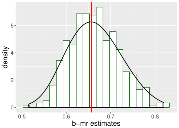
Figure 2: Estimates of b-mr when mr estimates go outside of [-1,1]. The red vertical line indicates the true value.

6 The causal effect of education on earnings

To illustrate the proposed methods, we reanalyze data from the National Longitudinal Survey of Young Men (NLS) (Card,, 1995; Tan,, 2006; Okui et al.,, 2012; Wang et al.,, 2017), which consist of observations on 5525 men aged between 14 and 24 in 1966. Among them, 3010 provided valid education and wage responses in the 1976 follow-up. We are interested in estimating the causal effect of education on earnings, which might be confounded by unobserved preferences for education levels. Card, (1995) proposes to use presence of a nearby 4-year college as an instrument. Following Tan, (2006), we consider education beyond high school as the treatment. In this data set, 2053 (68.2%) lived close to a 4-year college, and 1521 (50.5%) had education beyond high school. To illustrate the proposed methods with binary outcomes, we follow Wang et al., (2017) to dichotomize the outcome wage at its median, that is 5.375 dollars per hour.

We adjust for age, race, father and mother’s education levels, indicators for residence in the south and a metropolitan area and IQ scores, all measured in 1966. Among them, race, parents’ education levels and residence are included as they may affect both the instrument and outcome; age is included as it is likely to modify the effect of education on earnings, and IQ scores, as a measure of underlying ability, are included as they may modify both the effect of proximity to college on education, and the effect of education on earnings. Following Card, (1995), we use mean imputation for missing values, and include indicators of imputation in the models. The NLS was also not a representative sample of the US population. We account for this by reweighing observations using their sampling weights.

We first apply the test of Wang et al., (2017) to check the proposed instrumental variable model. Analysis results show that the proposed IV model cannot be falsified with the observed data. We then apply the proposed methods to estimate the causal effect of education on earnings. In addition to the estimators included in Section 5, we report the crude estimate which does not account for any confounding, and the Risk Difference Regression (RDReg) estimate (Richardson et al.,, 2017), which only accounts for observed confounders; the RDReg estimate was obtained using R package brm (Wang and Richardson,, 2016). We also report the two-stage least square (2SLS) estimate, which is believed to approximate the causal relation of interest (Angrist and Pischke,, 2008) despite not respecting the natural model constraints of a binary outcome. The results are summarized in Table 3, wherein the confidence intervals are obtained by quantile-based nonparametric bootstrap.

Table 3: Estimates of the effect of education beyond high school on earnings (dichotomized at median)

Method	Point Estimate	95% Confidence Interval
naive	0.122	(0.085,0.162)
RDReg	0.037	($-$0.009,0.080)
2SLS	0.469	(-0.140,1.327)
b-reg	0.849	(0.239,0.978)
b-ipw	0.424	($-$1.000,1.000)
g	0.079	($-$0.355,1.000)
mr	0.328	($-$60.394,65.339)
b-mr	0.344	($-$0.373,0.938)

Table 3 summarizes the results. The bootstrapped estimates are based on 1000 bootstrap samples. Both 2SLS and bounded multiply robust estimation yield substantially higher point estimates than Risk Difference Regression, suggesting that unmeasured confounding leads to a downward bias in the regression estimate of causal effect; this is consistent with previous findings using the log wage as the outcome (Card,, 1995; Okui et al.,, 2012). Unlike 2SLS, the confidence interval given by the bounded multiply robust estimation is contained within the interval [$-$1, 1], confirming boundedness of the proposed estimator. The bounded IV regression estimate is very close to 1, which is unlikely given that the outcome takes value 0 or 1. This is probably due to misspecification of one or more models contained in $\mathcal{M}_{1}$. Despite this possible misspecification, the multiply robust methods still yield reasonable estimates. This indicates that multiply robust estimation does provide some protection against model misspecification. Furthermore, the multiply robust estimates are close to the bounded IPW estimate. This suggests that the models in $\mathcal{M}_{2}$, that are $\delta^{D}(X;\beta)$ and $f(Z\mid X;\gamma)$, may be close to the truth (Tchetgen Tchetgen and Robins,, 2010).

7 Discussion

IV methods are widely used to identify causal effects in the presence of unmeasured confounding. In practice, applied researchers are primarily interested in estimating the ATE. In contrast, the majority of statistical IV literature focuses on estimating the LATE, a legitimate causal parameter but often of secondary interest. We address this discrepancy by proposing novel assumptions that allow for identification of the ATE. We have argued that our novel identification assumptions are often more plausible than previous assumptions as they do not place constraints on the observed data distribution and do not suffer from the same limitations as previous identification approaches. Nevertheless, our identification assumptions lead to the same observed data functional as previous methods targeting the ATE, so that our proposed estimators can also be used to estimate the ATE under previous identification frameworks.

In this paper we discuss in detail how to obtain bounded estimators of the additive ATE with binary outcomes. This is especially relevant as most previous semiparametric IV methods primarily deal with continuous outcomes. Correspondingly, it is of interest to develop bounded estimators of the LATE with binary outcomes. Our approach in this paper can also be extended to improve causal effect estimation in the case of the multiplicative ATE, as well as to the context of a failure time outcome under additive or multiplicative hazards models. Finally, we have focused on the case of binary instrument and treatment in this paper. Extension of the proposed methodology to the case of general instrument or treatment is an interesting topic for future research.

Appendix

A Proof of Theorem 1

To simplify notation, conditioning on $X$ is implicit in our proof. We first note that

$$\delta^{Y} =\sum\limits_{z=0,1}(2z-1)E[Y\mid Z=z]$$

$$=\sum\limits_{z=0,1}(2z-1)E_{U}E[Y\mid Z=z,U]\quad(Z\rotatebox[origin={c}]{90.0}{$\models$}U)$$

$$=\sum\limits_{z=0,1}(2z-1)E_{U}\left\{E[YD\mid Z=z,U]+E[Y(1-D)\mid Z=z,U]\right\}$$

$$=E_{U}\sum\limits_{z=0,1}(2z-1)\left\{E[Y(1)D\mid Z=z,U]+E[Y(0)(1-D)\mid Z=z,U]\right\}$$

$$=E_{U}\sum\limits_{z=0,1}(2z-1)\{E[Y(1)\mid Z=z,U]P(D=1\mid Z=z,U)+E[Y(0)\mid Z=z,U]P(D=0\mid Z=z,U)\}\ \ \ (Y(d)\rotatebox[origin={c}]{90.0}{$\models$}D\mid(Z,U))$$

$$=E_{U}\sum\limits_{z=0,1}(2z-1)\{E[Y(1)\mid U]P(D=1\mid Z=z,U)+E[Y(0)\mid U]P(D=0\mid Z=z,U)\}\ \ \ (Y(d)\rotatebox[origin={c}]{90.0}{$\models$}Z\mid U)$$

$$=E_{U}\left(E[Y(1)-Y(0)\mid U]\left\{E[D\mid Z=1,U]-E[D\mid Z=0,U]\right\}\right).$$ (17)

Under A5.a,

$$E[D\mid Z=1,U]-E[D\mid Z=0,U]=E[D\mid Z=1]-E[D\mid Z=0]=\delta^{D};$$

under A5.b,

$$E[Y(1)-Y(0)\mid U]=E[Y(1)-Y(0)].$$

and due to $Z\rotatebox[origin={c}]{90.0}{$\models$}U$, $E_{U}\left\{E[D\mid Z=1,U]-E[D\mid Z=0,U]\right\}=E[D\mid Z=1]-E[D\mid Z=0]=\delta^{D}.$ Hence under either A5.a or A5.b, $\delta^{Y}=\delta^{D}E[Y(1)-Y(0)].$ This concludes our proof.

B Interpretation of the average Wald estimand when A5.a and A5.b both fail

Proposition 3:

Suppose $U$ is univariate and that for all $X$, $E[Y(1)-Y(0)\mid U,X]$ and
$\left(E[D\mid Z=1,U,X]-E[D\mid Z=0,U,X]\right)/\left(E[D\mid Z=1,X]-E[D\mid Z=0,X]\right)$ are both non-decreasing/ non-increasing in $U$. Then the average Wald estimand

$$\Delta\geq ATE.$$

Furthermore, if $U$ is multivariate, then the conclusion still holds if the components of $U$ are conditionally independent given $X$.

The proof follows by noting that (17) implies

$$\delta(X)-ATE(X) =\dfrac{\delta^{Y}(X)}{\delta^{D}(X)}-ATE(X)$$

$$=\dfrac{1}{\delta^{D}(X)}\left(E_{U\mid X}\left(E[Y(1)-Y(0)\mid U,X]\left\{E[D\mid Z=1,U,X]-E[D\mid Z=0,U,X]\right\}\right)-\right.$$

$$\left.E_{U\mid X}\left(E[Y(1)-Y(0)\mid U,X]\right)E_{U\mid X}\left\{E[D\mid Z=1,U,X]-E[D\mid Z=0,U,X]\right\}\right)$$

$$=Cov_{U\mid X}\left(E[Y(1)-Y(0)\mid U,X],\dfrac{1}{\delta^{D}(X)}\left\{E[D\mid Z=1,U,X]-E[D\mid Z=0,U,X]\right\}\right).$$

1 Proof of Proposition 1

To simplify notation, conditioning on $X$ is implicit in our proof. It was shown in Bonet, (2001) that (3) characterizes all the constraints on the observed data law implied by the canonical IV assumptions A1^′ – A4. It is trivial to see that (3) do not impose restrictions on $f(Z).$ To show that they do not impose restrictions on $(P(Y=1\mid Z=z),P(D=1\mid Z=z))\equiv(p^{Y}_{z},p_{z}^{D})$, we need to show for any $p^{Y}_{z},p^{D}_{z}\in[0,1],$ there exists $(P(Y=y,D=d\mid Z=z),z,d,y=0,1)$ that satisfies (3). Let $x_{z}=P(Y=1,D=1\mid Z=z),$ then the constraints (3) can be rewritten as the following inequalities:

$$x_{1}+p_{0}^{D}-x_{0} \leq 1,$$

$$p_{1}^{Y}-x_{1}+1+x_{0}-p_{0}^{Y}-p_{0}^{D} \leq 1,$$

$$p_{1}^{D}-x_{1}+x_{0} \leq 1,$$

$$1+x_{1}-p_{1}^{Y}-p_{1}^{D}+p_{0}^{Y}-x_{0} \leq 1,$$

which are equivalent to the following constraint on $x_{1}-x_{0}$:

$$\max(p_{1}^{Y}-p_{0}^{Y}-p_{0}^{D},p_{1}^{D}-1)\leq x_{1}-x_{0}\leq\min(1-p_{0}^{D},p_{1}^{Y}+p_{1}^{D}-p_{0}^{Y}).$$ (S1)

It is not hard to verify that $\max(p_{1}^{Y}-p_{0}^{Y}-p_{0}^{D},p_{1}^{D}-1)\leq\min(1-p_{0}^{D},p_{1}^{Y}+p_{1}^{D}-p_{0}^{Y})$ so there always exist $(x_{1},x_{0})$ that satisfy (S1). This completes the proof for claim (i). To show (ii), note that A5.a or A5.b holds trivially if

$$U\rotatebox[origin={c}]{90.0}{$\models$}(Z,D,Y(1),Y(0),X)$$ (S2)

and that (S2) is not falsifiable from the observed data.

2 Proof of Proposition 2

The proof follows from noting the following results:

1. $\delta^{Y}(X)=\delta^{D}(X)\delta(X)\in(-1,1)$;

2. The mapping $(\delta^{D}(X),OP^{D}(X))$ is a diffeomorphism from $(-1,1)\times\mathbb{R}^{+}$ to $(0,1)^{2}$;

3. The mapping $(\delta^{Y}(X),OP^{Y}(X))$ is a diffeomorphism from $(-1,1)\times\mathbb{R}^{+}$ to $(0,1)^{2}$;

4. $P(Y=1\mid Z,X)$ is variation independent of $P(D=1\mid Z,X).$

The second and third steps follow from results in Richardson et al., (2017).

3 Proof of Theorem 2

Using standard theory on likelihood-based inference, one can show that under $\mathcal{M}_{1}$, $\hat{\alpha}_{\text{\it 2mle}}$ is asymptotically linear. With slight abuse of notation, we also use $\alpha$ to denote the true value of the parameter $\alpha$. Suppose that

$$\hat{\alpha}_{\text{\it 2mle}}=\alpha+\mathbb{P}_{n}IC_{\alpha}+o_{p}\left(1/{\sqrt{n}}\right),$$

where $IC_{\alpha}$ is the influence curve of $\hat{\alpha}_{\text{\it 2mle}}.$ We then have

$$\mathbb{P}_{n}\delta(X;\hat{\alpha}_{\text{\it 2mle}}) =\mathbb{P}_{n}\left\{\delta(X;\alpha)+\dfrac{\partial\delta(X;\alpha)}{\partial\alpha}(\hat{\alpha}_{\text{\it 2mle}}-\alpha)\right\}+\mathbb{P}_{n}o_{p}(\hat{\alpha}_{\text{\it 2mle}}-\alpha)$$

$$=\Delta+\mathbb{P}_{n}IC_{\Delta}+\mathbb{P}_{n}\left\{\dfrac{\partial\delta(X;\alpha)}{\partial\alpha}\left(\mathbb{P}_{n}IC_{\alpha}+o_{p}(1/{\sqrt{n}})\right)\right\}+o_{p}(1/\sqrt{n})$$

$$=\Delta+\mathbb{P}_{n}IC_{\Delta}+\left\{\mathbb{P}_{n}\dfrac{\partial\delta(X;\alpha)}{\partial\alpha}\right\}\left(\mathbb{P}_{n}IC_{\alpha}\right)+o_{p}(1/\sqrt{n})$$

$$=\Delta+\mathbb{P}_{n}IC_{\Delta}+E\left\{\dfrac{\partial\delta(X;\alpha)}{\partial\alpha}\right\}\left(\mathbb{P}_{n}IC_{\alpha}\right)+O_{p}(1//\sqrt{n})O_{p}(1//\sqrt{n})+o_{p}(1/\sqrt{n})$$

$$=\Delta+\mathbb{P}_{n}\left\{IC_{\Delta}+E\left\{\dfrac{\partial\delta(X;\alpha)}{\partial\alpha}\right\}IC_{\alpha}\right\}+o_{p}(1/\sqrt{n}),$$

where $IC_{\Delta}=\delta(X;\alpha)-\Delta$, and in the second and third steps above, we use the fact that for a given $n$, $\hat{\alpha}_{\text{\it 2mle}}$ does not depend on the specific unit $i$.

4 Proof of Theorem 3

We note that regardless of whether or not $\delta(X;\alpha)$ is correct, under $\mathcal{M}_{2}$ we have that both ($\hat{\beta}_{\text{\it ipw}},\hat{\Delta}_{\text{\it ipw}}$) and $(\hat{\beta}_{\text{\it ipw}},\hat{\Delta}_{\text{\it b-ipw}})$ solve equation (8) and the following equation:

$$\mathbb{P}_{n}\dfrac{Y}{\delta^{D}(X;\beta)}\dfrac{2Z-1}{f(Z\mid X;\hat{\gamma}_{\text{\it mle}})}-\Delta=0,$$ (S3)

wherein the maximum likelihood estimator $\hat{\gamma}_{\text{\it mle}}$ is consistent for $\gamma.$

Replacing $\hat{\gamma}_{mle}$ with $\gamma$, equation (8) is an unbiased estimating equation as

$$\quad E\left[h_{1}(X)\left(\dfrac{D(2Z-1)}{f(Z\mid X;\gamma)}-\delta^{D}(X;\beta)\right)\right]$$

$$=E_{X}h_{1}(X)E\left[\left.\dfrac{D(2Z-1)}{f(Z\mid X;\gamma)}-\delta^{D}(X;\beta)\right|X\right]$$

$$=E_{X}h_{1}(X)(\delta^{D}(X)-\delta^{D}(X;\beta))=0,$$

where the last line is due to the following identify:

$$\forall f,f(Z=1,X)-f(Z=0,X)=E\left[\left.f(Z,X)\dfrac{2Z-1}{f(Z\mid X)}\right|X\right].$$ (S4)

Similarly, replacing $\hat{\gamma}_{mle}$ with $\gamma$, equation (S3) is an unbiased estimating equation as because

$$\quad E\left[\dfrac{Y}{\delta^{D}(X;\beta)}\dfrac{2Z-1}{f(Z\mid X;\gamma)}\right]-\Delta$$

$$=E_{X}E\left[\left.\dfrac{Y}{\delta^{D}(X;\beta)}\dfrac{2Z-1}{f(Z\mid X;\gamma)}\right|X\right]-\Delta$$

$$=E_{X}\dfrac{\delta^{Y}(X)}{\delta^{D}(X)}-\Delta=0.$$

We now show that the equation (8) has a unique solution in the limit provided that i) the distribution of $X$ is non-degenerate; ii) $h_{1}(X)=X$. To see this, note that under these conditions,

$$\dfrac{\partial}{\partial\beta}E\left[h_{1}(X)\left(\dfrac{D(2Z-1)}{f(Z\mid X;\gamma)}-\delta^{D}(X;\beta)\right)\right]=\dfrac{4}{(e^{2\beta^{T}X}+1)^{2}}X^{T}X$$

is positive definite. One can also see from this proof that any choice of $h_{1}(X)$ that makes $(h_{1}(X))^{T}X$ positive definite would suffice.

The rest of the proof follows from standard M-estimation theory.

5 Proof of Theorem 5

In the following proof, we will use (S4) and the following identities repeatedly:

$$\forall f,E[f(X)S(Y\mid X)]=0;$$ (S5)

$$\forall f,E[f(X)(Y-E[Y\mid X])]=0,$$ (S6)

where $S(Y\mid X)$ is the score function corresponding to the conditional law of $Y$ given $X$.

To find the efficient influence function (EIF) for $\Delta$ in the union model $\mathcal{M}_{\text{\it union}}$, we first need to find a gradient in $\mathcal{M}_{\text{\it union}}$. To do so, we find the canonical gradient $G$ for $\Delta$ in the nonparametric model $\mathcal{M}_{\text{\it non}}$. Specifically, we aim to find a random variable $G$, such that $E[G]=0$ and for all one-dimensional parametric submodels of $\mathcal{M}_{\text{\it non}}$, denoted as $f(Y,D,Z,X;t)=f(Y,D\mid Z,X;t)f(Z\mid X;t)f(X;t)$, we have

$$\left.\dfrac{\partial}{\partial t}\Delta_{t}\right|_{t=0}=E[G\cdot S(Y,D,Z,X;t)]|_{t=0},$$ (S7)

where $S(Y,D,Z,X;t)=\partial\log f(Y,D,Z,X;t)/\partial t$ and

$$\dfrac{\partial}{\partial t}\Delta_{t}=\dfrac{\partial}{\partial t}\int\dfrac{\int y\ dF_{t}(y\mid Z=1,X)-\int y\ dF_{t}(y\mid Z=0,X)}{\int d\ dF_{t}(d\mid Z=1,X)-\int d\ dF_{t}(d\mid Z=0,X)}f_{t}(X)\ dX=\dfrac{\partial}{\partial t}E_{t}\left\{\dfrac{\delta^{Y}_{t}\left(X\right)}{\delta^{D}_{t}\left(X\right)}\right\}.$$

First note that

$$\left.\dfrac{\partial}{\partial t}\Delta_{t}\right|_{t=0} = \left.\dfrac{\partial}{\partial t}E_{t}\left\{\dfrac{\delta^{Y}_{t}\left(X\right)}{\delta^{D}_{t}\left(X\right)}\right\}\right|_{t=0}$$

$$= \left.E\left\{\dfrac{\delta^{Y}\left(X\right)}{\delta^{D}\left(X\right)}S(X)\right\}+E\left\{\dfrac{\dfrac{\partial}{\partial t}\delta^{Y}_{t}\left(X\right)\delta^{D}\left(X\right)-\delta^{Y}\left(X\right)\dfrac{\partial}{\partial t}\delta^{D}_{t}\left(X\right)}{(\delta^{D}\left(X\right))^{2}}\right\}\right|_{t=0}$$

$$= \left.E\left\{\dfrac{\delta^{Y}\left(X\right)}{\delta^{D}\left(X\right)}S(Y,D,Z,X)\right\}+E\left\{\dfrac{\dfrac{\partial}{\partial t}\delta^{Y}_{t}\left(X\right)\delta^{D}\left(X\right)-\delta^{Y}\left(X\right)\dfrac{\partial}{\partial t}\delta^{D}_{t}\left(X\right)}{(\delta^{D}\left(X\right))^{2}}\right\}\right|_{t=0}\text{\quad(following \eqref{identity_1})},$$

where $S(X)$ denotes the score function for $X$, and

$$\dfrac{\partial}{\partial t}E_{t}(Y\mid Z=z,X) =\dfrac{\partial}{\partial t}\int yf_{t}(y\mid Z=z,X)dy$$

$$={E\left[Y\dfrac{\dfrac{\partial}{\partial t}f_{t}(Y\mid Z=z,X)}{f_{t}(Y\mid Z=z,X)}\right]}$$

$$=E\left[(Y-E[Y\mid Z=z,X])S(Y\mid Z=z,X)\right]\text{\quad(following \eqref{identity_1})}$$

$$=E\left[(Y-E[Y\mid Z=z,X])S(Y,Z=z\mid X)\right]\text{\quad(following \eqref{identity_2})}.$$

Hence

$$\dfrac{\partial}{\partial t}\delta^{Y}_{t}\left(X\right) =\dfrac{\partial}{\partial t}\left\{E_{t}(Y\mid Z=1,X)-E_{t}(Y\mid Z=0,X)\right\}$$

$$=E\left[(Y-E[Y\mid Z=1,X])S(Y,Z=1\mid X)\right]-E\left[(Y-E[Y\mid Z=0,X])S(Y,Z=0\mid X)\right]$$

$$=E\left(\left.\dfrac{2Z-1}{f(Z\mid X)}\left(Y-E\left(Y|Z,X\right)\right)S(Y,Z\mid X)\,\right|\,X\right)\text{\quad(following \eqref{identity_3})}$$

$$=E\left(\left.\dfrac{2Z-1}{f(Z\mid X)}\left(Y-E\left(Y|Z,X\right)\right)S(Y,Z,X)\,\right|\,X\right)\text{\quad(following \eqref{identity_2})}$$

$$=E\left(\left.\dfrac{2Z-1}{f(Z\mid X)}\left(Y-E\left(Y|Z,X\right)\right)S(Y,D,Z,X)\,\right|\,X\right)\text{\quad(following \eqref{identity_1})}.$$

Similarly,

$$\dfrac{\partial}{\partial t}\delta^{D}_{t}\left(X\right)=E\left(\left.\dfrac{2Z-1}{f(Z\mid X)}\left(D-E\left(D|Z,X\right)\right)S(Y,D,Z,X)\,\right|\,X\right).$$

It then follows that

$$\tilde{G} = \dfrac{2Z-1}{f(Z\mid X)}\left(\dfrac{Y-E\left(Y|Z,X\right)}{\delta^{D}\left(X\right)}-\dfrac{\left(D-E\left(D|Z,X\right)\right)}{\delta^{D}\left(X\right)}\dfrac{\delta^{Y}\left(X\right)}{\delta^{D}\left(X\right)}\right)+\dfrac{\delta^{Y}\left(X\right)}{\delta^{D}\left(X\right)}$$

$$= \dfrac{2Z-1}{f(Z\mid X)}\dfrac{1}{\delta^{D}(X)}\left\{{Y-E\left(Y|Z,X\right)}-{\left(D-E\left(D|Z,X\right)\right)}\delta\left(X\right)\right\}+\delta\left(X\right)$$

$$= \dfrac{2Z-1}{f(Z\mid X)}\dfrac{1}{\delta^{D}(X)}\left\{{Y}-\delta\left(X\right)\delta^{D}(X)Z-{p_{0}^{Y}\left(X\right)}-{D}\delta\left(X\right)+Z\delta^{D}\left(X\right)\delta(X)+p_{0}^{D}(X){\delta\left(X\right)}\right\}+\delta\left(X\right)$$

$$= \dfrac{2Z-1}{f(Z\mid X)}\dfrac{1}{\delta^{D}(X)}\left\{{Y}-{p_{0}^{Y}\left(X\right)}-{D}\delta\left(X\right)+p_{0}^{D}(X){\delta\left(X\right)}\right\}+\delta\left(X\right)$$

satisfies (S7), in which we use the identities $E\left(Y|Z,X\right)=\delta\left(X\right)\delta^{D}\left(X\right)Z+p_{0}^{Y}\left(X\right)$ and $E\left(D|Z,X\right)=\delta^{D}\left(X\right)Z+p_{0}^{D}\left(X\right).$ Following (S4) one can show that $E[\tilde{G}]=\Delta$. Consequently, the canonical gradient in $\mathcal{M}_{\text{\it non}}$ is $G=\tilde{G}-\Delta$, which equals the EIF evaluated at observed data $(Y,D,Z,X)$, as shown by standard semiparametric efficiency theory (Bickel et al.,, 1998). Results in Robins and Rotnitzky, (2001) then show that the EIF in the union model $\mathcal{M}_{\text{\it union}}$ coincides with the EIF in $\mathcal{M}_{\text{\it non}}$. This concludes our proof.

6 Proof of Theorem 6

Under suitable regularity conditions (White,, 1982), the estimators $\hat{\alpha}_{\text{\it dr}},{\hat{\beta}_{\text{\it dr}}},\hat{\gamma}_{\text{\it mle}},\hat{\theta}_{\text{\it mle}},\hat{\iota}_{\text{\it mle}}$ converge in probability to fixed constants ${\alpha}^{\ast},{\beta}^{\ast},{\gamma}^{\ast},{\theta}^{\ast},{\iota}^{\ast}$ regardless of whether the corresponding models are correct or not. In the following, we denote $\delta(X;{\alpha}^{\ast})$ as $\delta^{\ast}(X)$. Likewise for the other models.

It suffices to show that ${\Delta}_{mr}^{*}$ has expectation $\Delta$ in the union model, where

$${\Delta}_{mr}^{*}=\mathbb{P}_{n}\left\{\dfrac{1}{\delta^{D}(X;{\beta}^{*}_{\text{\it dr}})}\left(Y-D\delta\left(X;{\alpha}^{*}_{\text{\it dr}}\right)-p_{0}^{Y}\left(X;{\iota}^{*}_{\text{\it mle}}\right)+p_{0}^{D}(X;{\theta}^{*}_{\text{\it mle}})\delta\left(X;{\alpha}^{*}_{\text{\it dr}}\right)\right)\dfrac{2Z-1}{f(Z\mid X;{\gamma}^{*}_{\text{\it mle}})}+\delta\left(X;{\alpha}^{*}_{\text{\it dr}}\right)\right\}.$$

Suppose only $\mathcal{M}_{1}$ holds such that $\delta^{\ast}\left(X\right)=\delta\left(X\right)$, $\delta^{D,\ast}(X)=\delta^{D}(X),p_{0}^{Y,\ast}\left(X\right)=p_{0}^{Y}\left(X\right)$ and $p_{0}^{D,\ast}(X)=p_{0}^{D}(X)$ but $f^{\ast}\left(Z\mid X\right)\neq f(Z\mid X)$. Then

$$E[{\Delta}_{\text{\it}mr}^{*}] = E\left\{\dfrac{2Z-1}{f^{\ast}\left(Z\mid X\right)}\dfrac{1}{\delta^{D}(X)}\left\{{Y}-{p_{0}^{Y}\left(X\right)}-{D}\delta\left(X\right)+p_{0}^{D}(X){\delta\left(X\right)}\right\}+\delta\left(X\right)\right\}$$

$$= E\left\{\dfrac{2Z-1}{f^{\ast}\left(Z\mid X\right)}\dfrac{1}{\delta^{D}(X)}\left\{{\delta\left(X\right)\delta^{D}(X)Z}-{Z\delta^{D}(X)}\delta\left(X\right)\right\}+\Delta\right\}$$

$$= \Delta.$$

Suppose instead only $\mathcal{M}_{2}$ holds such that $f^{\ast}\left(Z\mid X\right)=f(Z\mid X)$ and $\delta^{D,\ast}\left(X\right)=\delta^{D}(X)$ but $\delta^{\ast}\left(X\right)\neq\delta\left(X\right),p_{0}^{Y,\ast}\left(X\right)\neq p_{0}^{Y}\left(X\right)$ and $p_{0}^{D,\ast}(X)\neq p_{0}^{D}(X)$. Then

$$E[{\Delta}^{*}_{\text{\it}mr}] =E\left\{\dfrac{2Z-1}{f\left(Z\mid X\right)}\dfrac{1}{\delta^{D}(X)}\left({Y}-{p_{0}^{Y,\ast}\left(X\right)}-{D}\delta^{\ast}\left(X\right)+p_{0}^{D,\ast}\left(X\right){\delta^{\ast}\left(X\right)}\right)+\delta^{\ast}\left(X\right)\right\}$$

$$=E\left\{\dfrac{2Z-1}{f\left(Z\mid X\right)}\dfrac{1}{\delta^{D}(X)}\left({\delta\left(X\right)\delta^{D}(X)Z+p_{0}^{Y}(X)}-{p_{0}^{Y,\ast}\left(X\right)}-\left(\delta^{D}(X)Z+p_{0}^{D}(X)\right)\delta^{\ast}\left(X\right)+p_{0}^{D,\ast}\left(X\right){\delta^{\ast}\left(X\right)}\right)\right\}+$$

$$\quad E\left\{\delta^{\ast}\left(X\right)\right\}$$

$$=E\left\{\delta\left(X\right)-\delta^{\ast}\left(X\right)+\delta^{\ast}\left(X\right)\right\}=\Delta.$$

Finally suppose only $\mathcal{M}_{3}$ holds such that $f^{\ast}\left(Z\mid X\right)=f(Z\mid X)$ and $\delta^{*}\left(X\right)=\delta(X)$ but $\delta^{D,\ast}(X)\neq\delta^{D}(X),p_{0}^{Y,\ast}\left(X\right)\neq p_{0}^{Y}\left(X\right)$ and $p_{0}^{D,\ast}(X)\neq p_{0}^{D}(X)$. Then

$$E[{\Delta}^{*}_{\text{\it}mr}] =E\left\{\dfrac{2Z-1}{f\left(Z\mid X\right)}\dfrac{1}{\delta^{D,\ast}(X)}\left({Y}-{p_{0}^{Y,\ast}\left(X\right)}-{D}\delta\left(X\right)+p_{0}^{D,\ast}\left(X\right){\delta\left(X\right)}\right)+\delta\left(X\right)\right\}$$

$$=E\left\{\dfrac{2Z-1}{f\left(Z\mid X\right)}\dfrac{1}{\delta^{D,\ast}(X)}\left({\delta\left(X\right)\delta^{D}(X)Z+p_{0}^{Y}(X)}-{p_{0}^{Y,\ast}\left(X\right)}-\left(\delta^{D}(X)Z+p_{0}^{D}(X)\right)\delta\left(X\right)+p_{0}^{D,\ast}\left(X\right){\delta\left(X\right)}\right)\right\}+$$

$$\quad E\left\{\delta\left(X\right)\right\}$$

$$=E\left\{\dfrac{1}{\delta^{D,\ast}\left(X\right)}\left({\delta\left(X\right)\delta^{D}(X)}-{\delta\left(X\right)\delta^{D}\left(X\right)}\right)+\delta\left(X\right)\right\}=\Delta.$$

This concludes the proof for the first claim. The second claim in Theorem 6 follows from Theorem 5.

7 Additional simulation results

Table S1: Boxplots for the proposed estimators under all possible combinations of correct/incorrect specifications of the following four sets of models: $\delta(X),\delta_{D}(X),f(Z\mid X)$ and $OP(X)$, where $OP(X)=OP^{Y}(X),OP^{D}(X))$. The true value for the average Wald estimand is 0.087, annotated with the red horizontal lines. The sample size is 500

$(\pi(X),OP(X))$		$(\delta^{D}(X),\delta(X))$
		$(\checkmark,\checkmark)$	$(\checkmark,\times)$	$(\times,\checkmark)$	$(\times,\times)$
$(\checkmark,\checkmark)$
$(\checkmark,\times)$
$(\times,\checkmark)$
$(\times,\times)$

References

- Abadie, (2003) Abadie, A. (2003). Semiparametric instrumental variable estimation of treatment response models. Journal of Econometrics, 113(2):231–263.
- Abadie et al., (2002) Abadie, A., Angrist, J. D., and Imbens, G. W. (2002). Instrumental variables estimates of the effect of subsidized training on the quantiles of trainee earnings. Econometrica, 70(1):91–117.
- Angrist and Fernandez-Val, (2013) Angrist, J. D. and Fernandez-Val, I. (2013). Extrapolate-ing: External validity and overidentification in the LATE framework. In Acemoglu, D., Arellano, M., and Dekel, E., editors, Advances in Economics and Econometrics: Theory and Applications, Tenth World Congress, Volume III: Econometrics, pages 401–434. Cambridge, England: Cambridge University Press.
- Angrist et al., (1996) Angrist, J. D., Imbens, G. W., and Rubin, D. B. (1996). Identification of causal effects using instrumental variables. Journal of the American Statistical Association, 91:444–455.
- Angrist and Pischke, (2008) Angrist, J. D. and Pischke, J.-S. (2008). Mostly harmless econometrics: An empiricist’s companion. Princeton: Princeton University Press.
- Aronow and Carnegie, (2013) Aronow, P. M. and Carnegie, A. (2013). Beyond LATE: Estimation of the average treatment effect with an instrumental variable. Political Analysis, 21(4):492–506.
- Baker and Lindeman, (1994) Baker, S. G. and Lindeman, K. S. (1994). The paired availability design: a proposal for evaluating epidural analgesia during labor. Statistics in Medicine, 13(21):2269–2278.
- Balke and Pearl, (1997) Balke, A. and Pearl, J. (1997). Bounds on treatment effects from studies with imperfect compliance. Journal of the American Statistical Association, 92(439):1171–1176.
- Bickel et al., (1998) Bickel, P. J., Klaassen, C. A., Ritov, Y., and Wellner, J. A. (1998). Efficient and adaptive estimation for semiparametric models. New York: Springer-Verlag.
- Bonet, (2001) Bonet, B. (2001). Instrumentality tests revisited. In Proceedings of the Seventeenth conference on Uncertainty in artificial intelligence, pages 48–55. Morgan Kaufmann Publishers Inc.
- Card, (1995) Card, D. (1995). Using geographic variation in college proximity to estimate the return to schooling. In Christofides, L. N., Swidinsky, R., and Grant, E. K., editors, Aspects of Labour Market Behaviour: Essays in Honour of John Vanderkamp, pages 201–222. Toronto: University of Toronto Press.
- Cefalu et al., (2017) Cefalu, M., Dominici, F., Arvold, N., and Parmigiani, G. (2017). Model averaged double robust estimation. Biometrics, 73(2):410–421.
- Cheng et al., (2009) Cheng, J., Small, D. S., Tan, Z., and Ten Have, T. R. (2009). Efficient nonparametric estimation of causal effects in randomized trials with noncompliance. Biometrika, 96(1):19–36.
- Chesher, (2010) Chesher, A. (2010). Instrumental variable models for discrete outcomes. Econometrica, 78(2):575–601.
- Clarke and Windmeijer, (2012) Clarke, P. S. and Windmeijer, F. (2012). Instrumental variable estimators for binary outcomes. Journal of the American Statistical Association, 107(500):1638–1652.
- Dawid, (2003) Dawid, A. (2003). Causal inference using influence diagrams: the problem of partial compliance. In Green, P. J., Hjort, N. L., and Richardson, S., editors, Highly Structured Stochastic Systems, pages 45–65. Oxford, England: Oxford University Press.
- Deaton, (2009) Deaton, A. S. (2009). Instruments of development: Randomization in the tropics, and the search for the elusive keys to economic development. Technical report, National Bureau of Economic Research.
- Didelez and Sheehan, (2007) Didelez, V. and Sheehan, N. (2007). Mendelian randomization as an instrumental variable approach to causal inference. Statistical Methods in Medical Research, 16(4):309–330.
- Frangakis and Rubin, (1999) Frangakis, C. E. and Rubin, D. B. (1999). Addressing complications of intention-to-treat analysis in the combined presence of all-or-none treatment-noncompliance and subsequent missing outcomes. Biometrika, 86(2):365–379.
- Frangakis and Rubin, (2002) Frangakis, C. E. and Rubin, D. B. (2002). Principal stratification in causal inference. Biometrics, 58(1):21–29.
- Frölich, (2007) Frölich, M. (2007). Nonparametric IV estimation of local average treatment effects with covariates. Journal of Econometrics, 139(1):35–75.
- Goldberger, (1972) Goldberger, A. S. (1972). Structural equation methods in the social sciences. Econometrica, 40(6):979–1001.
- Han and Wang, (2013) Han, P. and Wang, L. (2013). Estimation with missing data: beyond double robustness. Biometrika, 100:417–430.
- Heckman and Urzua, (2010) Heckman, J. J. and Urzua, S. (2010). Comparing IV with structural models: What simple IV can and cannot identify. Journal of Econometrics, 156(1):27–37.
- Hernán and Robins, (2006) Hernán, M. A. and Robins, J. M. (2006). Instruments for causal inference: An epidemiologist’s dream? Epidemiology, 17(4):360–372.
- Imbens, (2010) Imbens, G. W. (2010). Better LATE than nothing. Journal of Economic Literature, 48(2):399–423.
- Imbens and Angrist, (1994) Imbens, G. W. and Angrist, J. D. (1994). Identification and estimation of local average treatment effects. Econometrica, 62(2):467–475.
- Li et al., (2017) Li, W., Gu, Y., and Liu, L. (2017). Demystifying multiply robust estimators. (under review).
- Liu et al., (2015) Liu, L., Miao, W., Sun, B., Robins, J. M., and Tchetgen Tchetgen, E. J. (2015). Identification and inference for marginal average treatment effect on the treated with an instrumental variable. arXiv preprint arXiv:1506.08149.
- Molina et al., (2017) Molina, J., Rotnitzky, A., Mariela, S., and Robins, J. M. (2017). Multiple robustness in factorized likelihood models. Biometrika, 104(3):561–581.
- Naik et al., (2016) Naik, C., McCoy, E. J., and Graham, D. J. (2016). Multiply robust estimation for causal inference problems. arXiv preprint arXiv:1611.02433.
- Neyman, (1923) Neyman, J. (1923). Sur les applications de la thar des probabilities aux experiences Agaricales: Essay des principle. English translation of excerpts by Dabrowska, D. and Speed, T. (1990). Statistical Science, 5:463–472.
- Ogburn et al., (2015) Ogburn, E. L., Rotnitzky, A., and Robins, J. M. (2015). Doubly robust estimation of the local average treatment effect curve. Journal of the Royal Statistical Society: Series B (Statistical Methodology), 77(2):373–396.
- Okui et al., (2012) Okui, R., Small, D. S., Tan, Z., and Robins, J. M. (2012). Doubly robust instrumental variable regression. Statistica Sinica, 22(1):173–205.
- Pearl, (1995) Pearl, J. (1995). On the testability of causal models with latent and instrumental variables. In Proceedings of the Eleventh conference on Uncertainty in artificial intelligence, pages 435–443. Morgan Kaufmann Publishers Inc.
- Pearl, (2009) Pearl, J. (2009). Causality. Cambridge, England: Cambridge University Press.
- Pearl, (2011) Pearl, J. (2011). Principal stratification – a goal or a tool? The International Journal of Biostatistics, 7(1):20.
- Richardson and Robins, (2013) Richardson, T. S. and Robins, J. M. (2013). Single world intervention graphs (SWIGs): A unification of the counterfactual and graphical approaches to causality. Center for the Statistics and the Social Sciences, University of Washington Series. Working Paper, 128.
- Richardson and Robins, (2014) Richardson, T. S. and Robins, J. M. (2014). ACE bounds; SEMs with equilibrium conditions. Statistical Science, 29(3):363–366.
- Richardson et al., (2017) Richardson, T. S., Robins, J. M., and Wang, L. (2017). On modeling and estimation for the relative risk and risk difference. Journal of the American Statistical Association, 519:1121–1130.
- Robins, (1994) Robins, J. M. (1994). Correcting for non-compliance in randomized trials using structural nested mean models. Communications in Statistics-Theory and Methods, 23(8):2379–2412.
- Robins and Greenland, (1996) Robins, J. M. and Greenland, S. (1996). Identification of causal effects using instrumental variables: comment. Journal of the American Statistical Association, 91(434):456–458.
- Robins and Rotnitzky, (2001) Robins, J. M. and Rotnitzky, A. (2001). Comment on “Inference for semiparametric models: Some questions and an answer,” by P.J. Bickel and J. Kwon. Statistica Sinica, 11:920–936.
- Robins et al., (2007) Robins, J. M., Sued, M., Lei-Gomez, Q., and Rotnitzky, A. (2007). Comment: Performance of double-robust estimators when “inverse probability” weights are highly variable. Statistical Science, 22(4):544–559.
- Rubin, (1974) Rubin, D. B. (1974). Estimating causal effects of treatments in randomized and nonrandomized studies. Journal of Educational Psychology, 66(5):688.
- Rubin, (1980) Rubin, D. B. (1980). Comment. Journal of the American Statistical Association, 75(371):591–593.
- Rubin, (2007) Rubin, D. B. (2007). The design versus the analysis of observational studies for causal effects: parallels with the design of randomized trials. Statistics in Medicine, 26(1):20–36.
- Tan, (2006) Tan, Z. (2006). Regression and weighting methods for causal inference using instrumental variables. Journal of the American Statistical Association, 101(476):1607–1618.
- Tan, (2010) Tan, Z. (2010). Bounded, efficient and doubly robust estimation with inverse weighting. Biometrika, 97(3):661–682.
- Tchetgen Tchetgen, (2009) Tchetgen Tchetgen, E. J. (2009). A commentary on G. Molenberghs’s review of missing data methods. Drug Information Journal, 43(4):433–435.
- Tchetgen Tchetgen and Robins, (2010) Tchetgen Tchetgen, E. J. and Robins, J. M. (2010). The semiparametric case-only estimator. Biometrics, 66(4):1138–1144.
- Tchetgen Tchetgen et al., (2010) Tchetgen Tchetgen, E. J., Robins, J. M., and Rotnitzky, A. (2010). On doubly robust estimation in a semiparametric odds ratio model. Biometrika, 97(1):171–180.
- Tchetgen Tchetgen and Shpitser, (2012) Tchetgen Tchetgen, E. J. and Shpitser, I. (2012). Semiparametric theory for causal mediation analysis: efficiency bounds, multiple robustness, and sensitivity analysis. Annals of Statistics, 40(3):1816–1845.
- Tchetgen Tchetgen and Vansteelandt, (2013) Tchetgen Tchetgen, E. J. and Vansteelandt, S. (2013). Alternative identification and inference for the effect of treatment on the treated with an instrumental variable. Harvard University Biostatistics Working Paper Series. Working Paper 166.
- Theil, (1953) Theil, H. (1953). Repeated least squares applied to complete equation systems. The Hague: central planning bureau.
- VanderWeele, (2008) VanderWeele, T. J. (2008). The sign of the bias of unmeasured confounding. Biometrics, 64(3):702–706.
- Vansteelandt and Didelez, (2015) Vansteelandt, S. and Didelez, V. (2015). Robustness and efficiency of covariate adjusted linear instrumental variable estimators. arXiv preprint arXiv:1510.01770.
- Vansteelandt et al., (2007) Vansteelandt, S., Rotnitzky, A., and Robins, J. (2007). Estimation of regression models for the mean of repeated outcomes under nonignorable nonmonotone nonresponse. Biometrika, 94(4):841–860.
- Vansteelandt et al., (2008) Vansteelandt, S., VanderWeele, T. J., Tchetgen Tchetgen, E. J., and Robins, J. M. (2008). Multiply robust inference for statistical interactions. Journal of the American Statistical Association, 103(484):1693–1704.
- Vermeulen and Vansteelandt, (2015) Vermeulen, K. and Vansteelandt, S. (2015). Bias-reduced doubly robust estimation. Journal of the American Statistical Association, 110(511):1024–1036.
- Wald, (1940) Wald, A. (1940). The fitting of straight lines if both variables are subject to error. The Annals of Mathematical Statistics, 11(3):284–300.
- Wang and Richardson, (2016) Wang, L. and Richardson, T. (2016). brm: Binary Regression Model. R package version 1.0.
- Wang et al., (2017) Wang, L., Robins, J. M., and Richardson, T. S. (2017). On falsification of the binary instrumental variable model. Biometrika, 104(1):229–236.
- White, (1982) White, H. (1982). Maximum likelihood estimation of misspecified models. Econometrica, 50:1–25.
- Wooldridge, (2010) Wooldridge, J. M. (2010). Econometric analysis of cross section and panel data. Cambridge, MA: MIT Press.
- Wright and Wright, (1928) Wright, P. G. and Wright, S. (1928). The tariff on animal and vegetable oils. New York: The Macmillan Co.
Supplementary Materials for