Pulsed entanglement of two optomechanical oscillators

Abstract

A strategy for generating entanglement in two separated optomechanical oscillators is analysed, using entangled radiation produced from downconversion and stored in an initiating cavity. We show that the use of pulsed entanglement with optimally shaped temporal modes can efficiently transfer quantum entanglement into a mechanical mode, then remove it after a fixed waiting time for measurement. This protocol could provide new avenues to test for bounds on decoherence in massive systems that are spatially separated, as originally suggested by Furry furry not long after the discussion by Einstein-Podolsky-Rosen (EPR) and Schrödinger of entanglement.

Macroscopic mechanical oscillators have now been cooled to their quantum ground state cooling_Connell_2010_Nature ; cooling_Chan_2011_Nature ; cooling_Gro_2009_NP ; cooling_Teufel , followed by the observations of macroscopic quantum effects quantum_macro ; quantum_macro2 ; quantum_macro3 ; quantum_macro4 including quantum entanglement Palomaki between a mechanical oscillator and a radiation field. Even more spectacular demonstrations of macroscopic quantum properties will soon become achievable. An important goal is to demonstrate long-lived entanglement between two separated mechanical systems. This would enable new tests of quantum mechanics, including the possible decoherence of quantum correlations due to space-like separation.

The intriguing idea of spatially dependent decoherence furry was first advanced by Furry just after the publication of the original EPR paradox EPR1935 and entanglement papers Schrodinger . Furry’s hypothesis is not predicted by conventional reservoir theory. It could occur in a modified quantum mechanics, including quantum gravity or other type of intrinsic decoherence Pearle ; GRW ; Penrose ; Diosi . It is clear from experiments in quantum optics that spatially dependent decoherence does not occur for massless photons Delft_2015 . However, there are no measurements yet on entanglement decay when massive, separated objects have an entangled center-of-mass motion. The success of quantum optomechanical entanglement and gravity-wave detectors LIGO_2013 demonstrates that such experiments are ideal for investigating previously accessible questions like this.

In this Letter, we propose and analyse a simple pulsed protocol for creating and measuring such macroscopic entanglement. The basic experimental setup involves an entangled source and spatially separated quantum optomechanical systems. An optical parametric amplifier creates two entangled modes Reid1989 ; Reid-Drumm ; EPR-exp ; rmp , ideally with the same frequency and different polarizations. This entanglement is transferred, on demand, to the separated quantum optomechanical systems – thus destroying the initial entanglement in optical modes. The entangled mechanical modes are stored, subsequently coupled out and measured optically, as indicated schematically in Fig (1). There are other proposals for entangling quantum optomechanical systems ent-opto-Giovannetti ; ent-opto-Mancini ; ent-opto-Hofer ; ent_proposal-eanglement-criteria-He2013 , but the lifetime of quantum entanglement and spatial separation are not controllable with these proposals. These requirements appear essential to a test of Furry’s hypothesis.

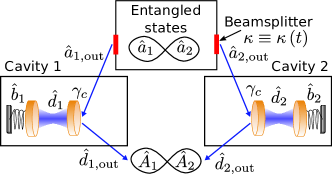
Figure 1: Schematic diagram of entanglement protocol.

The entangled source cavity modes $a_{1}$ and $a_{2}$ are assumed to be initially in a two mode squeezed state, prepared using the standard technique of nondegenerate parametric down-conversion. To give a definite model, this entangled state is initially prepared in a source cavity whose entanglement is characterized by a squeezing parameter $r$. The source cavity has tunable decay rates $\kappa\left(t\right)$, generating shaped, entangled outputs sech_pulse_He2009 ; other methods for state preparation are also possible.

The outputs are fed cascade_kolobov_1987 ; cascade_carmichael_1993 ; cascade_gardiner_1993 into the quantum optomechanical systems labelled Cavity $1$ and Cavity $2$, respectively, assuming identical optomechanical parameters. We linearize the equations of motion for an adiabatic ent-opto-Giovannetti ; ent-opto-Mancini pulsed optomechanical Hamiltonian describing these devices fast-coupling-Vanner2011 ; ent-opto-Hofer ; fast-coupling-Pikovski-np2012 ; KHDR , including dissipation and thermal noise for the cavity and mechanical modes. A time dependent optomechanical interaction $g\left(t\right)$ quantum_memory_He2009 allows the entangled modes to transfer to and from the mechanical modes $\hat{b}_{1}$ and $\hat{b}_{2}$. The output fields are then shaped optimally to match the $\operatorname{sech}$-shaped inputs, for maximum retrieval efficiency quantum_memory_He2009 ; sech_pulse_He2009 , with subsequent measurement of the stored entanglement.

Time-dependent coupling and decay

The optomechanical systems are modeled using the standard single mode theory Hamil_Brag ; Hamil_pierre ; Pace-Collett-Walls , following techniques explained in previous papers KHDR . It is convenient to introduce a dimensionless time variable, $\tau=\Gamma_{c}t$, relative to the optomechanical cavity decay rate $\Gamma_{c}$. To obtain universally valid results covering a range of different cases, all other times, frequencies and couplings are given in dimensionless units with derivatives $\dot{f}\equiv\partial f/\partial\tau$.

The equations of motion for the source cavity modes $a_{1},a_{2}$, are obtained in the absence of thermal noise, assuming the only losses are due to input/output coupling with a transmissivity $\kappa\left(\tau\right)$. Using input-output theory, with inputs $a_{k,\text{in}}$ and outputs $a_{k,\text{out}}$ one obtains inout-Gardiner-Collett ; inout_Yurke :

$$\dot{a}_{k} = -\kappa\left(\tau\right)a_{k}+\sqrt{2\kappa\left(\tau\right)}a_{k,\text{in}}$$

$$a_{k,\text{out}} \equiv \sqrt{2\kappa\left(\tau\right)}a_{k}-a_{k,\text{in}}.$$ (1)

We wish to generate a sech-shaped output pulse, $a_{out}\propto\operatorname{sech}\left(\tau\right)$. This is achieved using a dimensionless mirror transmissivity defined according to $\kappa\left(\tau\right)=\left[1+\tanh\left(\tau\right)\right]/2.$ We solve for Eq. (1) , giving

$$a_{k} = a_{k}\left(-\infty\right)\sqrt{\left[\frac{1-\tanh\left(\tau\right)}{2}\right]}+a_{vac}$$

$$a_{k,out} = \frac{a\left(-\infty\right)}{\sqrt{2}}\operatorname{sech}\left(\tau\right)+a^{\prime}_{vac}\,.$$ (2)

The operators $a_{\text{vac}}$, $a^{\prime}_{\text{vac}}$ are the source input and output vacuum noises respectively. The cavities are cascaded, so $d_{k,\text{in}}=a_{k,\text{out}}$, and from the input-output relations, $d_{k,\text{out}}\equiv\sqrt{2}d_{k}-d_{k,\text{in}}.$ The optomechanical systems satisfy the standard quantum Langevin equations Pace-Collett-Walls ; KHDR with cavity detuning $\delta\omega$, mechanical loss $\gamma_{m}$, and optomechanical coupling $\chi$, in dimensionless units.

Assuming an intense red-detuned pump with $\delta\omega=\omega_{m}$, and a resulting adiabatic coupling of $g=i\chi E/\left(\Gamma_{c}+i\delta\omega\right)$, the linearized Hamiltonian for cavities $1$ and $2$ is $\hat{H}_{a,k}/\hbar\approx i\left(g^{*}d_{k}b_{k}^{\dagger}-gd_{k}^{\dagger}b_{k}\right)$. Here, $d_{k}$ is a small fluctuation around the steady state in a frame rotating with detuning $\delta\omega$. We determine the time dependence of the optomechanical interaction strengths $g\left(\tau\right)$ of cavities $1$ and $2$, using previous work on quantum memories sech_pulse_He2009 .

To understand the mode-matching method, we start by analysing the linearized equations without losses in the mechanical oscillator, and without vacuum noise terms. These will be included in the full numerical analysis, given next. At this stage, we have that:

$$\dot{d}_{k} = -d_{k}-ig\left(\tau\right)b_{k}+\sqrt{2}d_{k,\text{in}}$$

$$\dot{b}_{k} = -ig\left(\tau\right)d_{k}\,.$$ (3)

To find conditions for perfect input coupling, we require that $d_{\text{out}}=0$ in the absence of vacuum noise. Hence $d_{k,\text{in}}=\sqrt{2}d_{k}$, leading to $\dot{d}_{k}=d_{k}-ig\left(\tau\right)b_{k}$. If we further assume $b_{-\infty}=0$, again neglecting vacuum noise, then it follows that $-ig\left(\tau\right)=\dot{b_{k}}/d_{k}$, giving

$$\left(\dot{d_{k}}+igb_{k}\right)/d_{k} = \dot{d_{k}}/d_{k}-\left(\dot{b}^{2}\right)/\left(2d_{k}^{2}\right)=1\,.$$ (4)

Now we note that $d_{k}=a\left(-\infty\right)\operatorname{sech}\left(\tau\right)/2$, and solving Eq. (4) gives us $b_{k}=ia\left(-\infty\right)\left[1+\tanh\left(\tau\right)\right]/2$. From $-ig\left(\tau\right)=\dot{b_{k}}/d_{k}$, we obtain the input modulation requirement of $g\left(\tau\right)=-\operatorname{sech}\left(\tau-\tau_{1}\right)$, where $\tau_{1}$ is the peak transmission of the input. The output modulation is identical apart from a shifted time-origin, from the symmetry of the input/output relations under interchange of the input and output terms.

Output modes $\hat{A}_{1},\hat{A}_{2}$

Detecting the stored entanglement requires an output measurement on temporal modes ${\displaystyle\hat{A}_{k}=\int_{-\infty}^{\infty}u_{k}\left(\tau^{\prime}\right)\hat{d}_{\text{out}}\left(\tau^{\prime}\right)d\tau^{\prime}}$ such that $\left[\hat{A}_{k},\hat{A}_{k}^{\dagger}\right]=1$ ent-opto-Hofer . We can then observe entanglement between $\hat{A}_{1}$ and $\hat{A}_{2}$ on a scale comparable with the initial entanglement between $\hat{a}_{1}$ and $\hat{a}_{2}$. Choosing the output pulse to be an identical shape to the input, so that $\hat{a}_{k,\text{out}}\propto\operatorname{sech}\left(\tau\right),$ we have $u_{k}\left(\tau\right)=u\left(\tau\right)=N\cdot\operatorname{sech}\left(\tau\right)$. This leads to a normalization of

$${\displaystyle N=1/\sqrt{\int_{-\infty}^{\infty}\operatorname{sech}\left(\tau\right)^{2}d\tau}=\sqrt{\frac{1}{2}}}\,,$$ (5)

The normalization constant for a restricted time-domain can also be found, which leads to minor corrections.

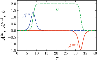
Figure 2: Temporal behaviour of the input field $a_{in}$, the output field $A_{out}$ and the mechanical state $b$.

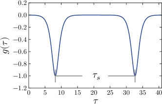
Figure 3: Temporal behaviour of the coupling strength.

Wigner representation and stochastic equations

There is thermal noise in the mechanical mode due to the interaction with its reservoir. In order to calculate these effects, and to include vacuum noise terms rigorously, it is useful to introduce a Wigner representation of the system density matrix Wigner ; Wigner_Castin ; Wigner_Steel . The Wigner function for the initial entangled state is given by Walls_book

$${\displaystyle W\left(\alpha_{+},\alpha_{-},\tau_{0}\right)=\frac{4}{\pi^{2}}\exp\left[-2\left(\frac{\left|\alpha_{+}\right|^{2}}{e^{2r}}+\frac{\left|\alpha_{-}\right|^{2}}{e^{-2r}}\right)\right]\,,}$$ (6)

where $\alpha_{\pm}{\displaystyle=\left(\alpha_{1}\pm\alpha_{2}^{*}\right)/\sqrt{2}}$ and $r$ is the squeezing parameter that characterizes the degree of entanglement. One can sample $\alpha_{1},\alpha_{2}$ by generating Gaussian noise vectors $\xi_{x}^{\pm},\xi_{y}^{\pm}$ with unit variance, defining $\alpha_{\pm}{\displaystyle=\left[\xi_{x}^{\pm}+i\xi_{y}^{\pm}\right]e^{\pm r}/2}$ and then obtaining mode amplitudes ${\displaystyle\alpha_{1}}=\left(\alpha_{+}+\alpha_{-}\right)/\sqrt{2}$ and ${\displaystyle\alpha_{2}}=\left(\alpha_{+}^{*}-\alpha_{-}^{*}\right)/\sqrt{2}$.

Quantum dynamical time evolution now follows a stochastic equation, after truncating third order derivative terms which are negligible for large occupation numbers. It is also possible to use a positive-P representation, which requires no truncation KHDR . Taking account of the cascaded input-output relations, the coupled equations describing time evolution of the Wigner amplitudes for the entangled source cavities $\alpha_{k}$, optical cavities $\delta_{k}$ and mechanical modes $\beta_{k}$ are given, for $k=1,2$, by

$$\dot{\alpha}_{k} = -\kappa\left(\tau\right)\alpha_{k}+\sqrt{2\kappa\left(\tau\right)}\xi_{k}$$

$$\dot{\delta}_{k} = -\delta_{k}-ig\left(\tau\right)\beta_{k}+2\sqrt{\kappa\left(\tau\right)}\alpha_{k}-\sqrt{2}\xi_{k}$$

$$\dot{\beta}_{k} = -\gamma_{m}\beta_{k}-ig\left(\tau\right)\delta_{k}+\sqrt{2\gamma_{m}\left(2\bar{n}_{\text{th},m}+1\right)}\xi_{2+k}\,.$$ (7)

Here $\bar{n}_{\text{th},m}=1/\left[\exp\left(\hbar\Gamma_{c}\omega_{m}/k_{B}T\right)-1\right]$ is the average phonon number in the mechanical bath, and $\xi_{k}$ are complex Gaussian noises with variances that correspond to the ’half-quanta’ occupations of symmetric Wigner vacuum correlations, $\langle\xi_{k}\left(\tau\right)\xi_{l}^{*}\left(\tau^{\prime}\right)\rangle=\frac{1}{2}\delta_{kl}\delta\left(\tau-\tau^{\prime}\right)$. Using the input-output relations again, we obtain the expression $\delta_{k,\text{out}}=\sqrt{2}\delta_{k}-\sqrt{2\kappa\left(\tau\right)}\alpha_{k}+\xi_{k}$. The output modes used for detecting entanglement are then:

$${\displaystyle A_{k,\text{out}}} =\int_{\tau_{1}+\tau_{s}/2}^{\tau_{\text{max}}}u\left(\tau-\tau_{2}\right)$$ (8)

$$\,\,\,\,\times\left(\left[\sqrt{2}\delta_{k}-\sqrt{2\kappa\left(\tau\right)}\alpha_{k}\right]+\xi_{k}\right)d\tau\,.$$

Note that the time integration for the output modes only starts after the first transfer pulse has been completed.

Experimental parameters

We assume that the optical modes of cavities $1$ and $2$ are initially in a vacuum state. The source cavity and cavities $1$ and $2$ are connected by a perfect, lossless waveguide. There is only one source of decoherence affecting the optical cavity modes, which is thermal noise in the mechanical modes.

Our simulations used experimental parameter values very similar to the optomechanical experiment values reported by Chan et. al. cooling_Chan_2011_Nature . The mechanical modes have an initial occupation of $n_{th,b}\left(0\right)=0.7$, corresponding to a reservoir temperature of $200\,\text{mK}$. The cavity decay rate is $\Gamma_{c}/2\pi=0.26\ \text{GHz}$. Relative to this time-scale, the mechanical oscillator has dimensionless resonance frequency $\omega_{m}/2\pi=14.23$, with a mechanical dissipation rate of $\gamma_{m}/2\pi=1.59\cdot 10{}^{-5}$ and an optomechanical coupling strength of $\chi_{0}/2\pi=3.5\times 10^{-3}$, which justifies the linearization ent-opto-Giovannetti ; ent-opto-Mancini and adiabatic approximations ent-opto-Hofer .

The time dependent source cavity decay rate that shapes the entangled modes is given by ${\displaystyle\kappa\left(\tau\right)=\frac{1}{2}\left[1+\tanh\left(\tau-\tau_{1}\right)\right]}$, while the effective coupling strength is

$$g\left(\tau\right) =\begin{cases}&-\sqrt{2}u\left(\tau-\tau_{1}\right)\,,\forall\,0\leq\tau\leq\tau_{1}+\frac{\tau_{s}}{2}\\ &-\sqrt{2}u\left(\tau-\tau_{2}\right)\,,\forall\,\tau_{1}+\frac{\tau_{s}}{2}\leq\tau\leq\tau_{\text{max}}\,,\end{cases}$$ (9)

where $\tau_{1}=8.17$ and $\tau_{2}=\tau_{1}+\tau_{s}$ are the dimensionless times when the storing and reading pulses peak, and $\tau_{\text{max}}=2\tau_{1}+\tau_{s}$, while $\tau_{s}$ is the dimensionless time between the peaks of the storage and readout pulses. It is also the storage time of the entangled state in the mechanical mode, as illustrated in Fig. 3.

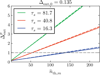
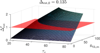
Figure 4: Entanglement as a function of temperature and storage time. The squeezing parameter is $r=1$, characterizing the degree of entanglement in the source cavity, while $\Delta_{\text{ent},0}=0.135$ is the initial value of entanglement.

Entanglement criterion

We use the phase- and gain-optimized product signature as an entanglement criterion entanglement-criteria-Giovanetti2003 , defined as:

$${\displaystyle\Delta_{ent}^{p}=\frac{4\Delta\left(X_{1}-GX_{2}^{\theta}\right)\Delta\left(P_{1}+GP_{2}^{\theta}\right)}{\left(1+G^{2}\right)}<1}\,,$$ (10)

where ${\displaystyle X_{k}^{\theta}}=\frac{1}{2}\left[e^{-i\theta}A_{k,\text{out}}+e^{i\theta}A_{k,\text{out}}^{\dagger}\right]$, $P_{k}^{\theta}=X_{k}^{\theta+\pi/2}$ and $G$ is an adjustable real constant. In particular, ${\displaystyle X_{k}=X_{k}^{0}}$, ${\displaystyle P_{k}=P_{k}^{0}}$ are the usual phase and amplitude quadratures. We minimize $\Delta_{\text{ent}}^{p}$ with respect to the gain $G$ and phase $\theta$ simultaneously. When inequality (10) holds, the optimised value of $\Delta_{\text{ent}}^{p}$ characterizes the degree of quantum entanglement between the modes entmeasPPT .

We compute $\Delta_{\text{ent}}^{p}$ in Eq. (10) as a function of thermal reservoir occupation number for a set of different storage times and a fixed squeezing parameter. To give an approximate analytic prediction, we consider only the degradation of the entanglement during its storage period in the mechanical oscillators. Using results described in epr_decoherence , we predict an entanglement value of

$$\Delta_{\text{ent}}^{p} =e^{-2\gamma_{m}\tau_{s}}e^{-2r}+\left(1-e^{-2\gamma_{m}\tau_{s}}\right)\left(1+2\bar{n}_{\text{th},m}\right)\,.$$ (11)

Fig. (4) shows the predicted entanglement results for squeezing parameter $r=1$ and three different storage times $\tau_{s}=16.3,\ 40.8,\ 81.7$, corresponding to $10\textrm{\,ns}$, $25\,\textrm{ns}$ and $50\,\textrm{ns}$, respectively. The solid lines indicate simulation results and dashed lines theoretical predictions.

The simulation results were obtained by solving Eqs. (7) with a stochastic $4$th order Runge-Kutta algorithm, $3000$ time-steps and $\approx 2\cdot 10^{8}$ samples, using open-source software Kiesewetter . They are in good agreement with our analytic predictions, in fact exhibiting slightly more favorable entanglement. A larger initial entanglement in the source cavity and a shorter storage time gives even better output temporal mode entanglement.

Quantum fidelity

We consider the quantum fidelity measure $\mathcal{F}=\langle\psi|\rho|\psi\rangle\,$, where $|\psi\rangle$ is the two mode squeezed state and $\rho$ is the density operator describing the temporal output modes. The fidelity quantifies the efficiency of our entanglement protocol as the entanglement in output temporal modes rely on successful entangled state transfer from the source cavity. In the Wigner representation fidelity_cahill_1969 ; fidelity_schumacher1996 ,

$$\mathcal{F}=\pi^{2}\int\ W_{\psi}\left(\alpha_{1},\alpha_{2}\right)W_{\rho}\left(\alpha_{1},\alpha_{2}\right)\ d^{2}\alpha_{1}d^{2}\alpha_{2}\,.$$ (12)

From the quantum simulations, we obtain sampled temporal output modes from the Wigner function $W_{\rho}$. The quantum fidelity $\mathcal{F}$ is then computed using

$$\mathcal{F} = \frac{\pi^{2}}{N_{\text{sample}}}\sum_{i}W_{\psi}\left(A_{1,\text{out}}^{i},A_{2,\text{out}}^{i}\right)\,,$$ (13)

where $A_{k,\text{out}}^{i}$ is the $i$th sample of temporal output mode $A_{k,\text{out}}$ and $N_{\text{sample}}$ is the total number of samples taken.

The quantum fidelity in Eq. (13) is also computed as a function of reservoir temperature and storage time. The top plot in Fig. (5) shows the steep drop in fidelity as storage time is increased. Comparing plots in Fig. (4) and Fig. (5) shows that a fidelity $\mathcal{F}$ of at least about $0.3$ is needed for entangled output modes.

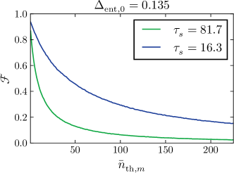
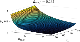
Figure 5: Fidelity $\mathcal{F}$ as a function of the thermal bath occupation number and storage time. Other parameters as in Fig 4.

EPR-steering

In addition to entanglement, we also analyze the stronger, asymmetric nonlocality signature known as the EPR-steering that links directly to the EPR paradox Reid1989 ; EPR1935 ; Wisemansteering . We use the CV signature for steering of system $1$ by system $2$ Reid1989

$$EPR_{1|2} = 4\Delta\left(X_{1}-GX_{2}^{\theta}\right)\Delta\left(P_{1}+GP_{2}^{\theta}\right)<1\,,$$ (14)

with $X,\>P$ as previously and an optimized gain $G$. Fig. 6 shows the predicted results for EPR-steering. The solid lines indicate simulation results and the dashed lines give analytic predictions. The analytic predictions were obtained analogously to the entanglement predictions. Using the results described in epr_decoherence , we obtain

$$EPR_{1|2} =\frac{2ab\left(1-b\right)c+b^{2}+c^{2}\left(1-b\right)^{2}}{ab+\left(1-b\right)c}\,,$$ (15)

where $a\equiv\cosh\left(2r\right),\ b\equiv e^{-2\gamma_{m}\tau_{s}},\ c\equiv\left(1+2\bar{n}_{\text{th},m}\right)\,$. Because of the symmetric setup, $EPR_{1|2}$ and $EPR_{2|1}$ are equal in magnitude.

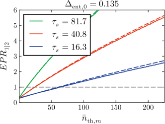
Figure 6: EPR-steering as a function of the thermal bath occupation number for three different storage times. Other parameters as in Fig 4.

Conclusions

In summary, our results show that a synchronous pulsed experiment can, in principle, transfer, store and read out macroscopic entanglement of two mechanical oscillators with nearly $100\%$ efficiency under ideal conditions. Due to finite temperature effects and damping, this effect is degraded in a predictable way. We calculate the quantitative effects of known decoherence on this proposed experiment. The experimental objectives would be to place a bound on additional decoherence that may occur due to the oscillator separation, to test the validity of Furry’s hypothesis.

- (1) W. H. Furry, Phys. Rev. 49, 393 (1936).
- (2) A. D. O’Connell et al., Nature 464, 697 (2010).
- (3) J. Chan et al., Nature 478, 89 (2011).
- (4) S. Groblacher et al., Nature Physics 5, 485 (2009).
- (5) J. D. Teufel et al., Nature 475, 359 (2011); 471, 204 (2011).
- (6) A. Safavi-Naeini et al, Phys. Rev. Lett. 108, 033602 (2012).
- (7) N. Brahms, T. Botter, S. Schreppler, D. W. C. Brooks, D. M. Stamper-Kurn, Phys. Rev. Lett. 108, 133601 (2012).
- (8) T. J. Kippenberg and K. J. Vahala, Science 321, 1172 (2008).
- (9) M. Aspelmeyer et al., J. Opt. Soc. Am. B 27, A189 (2010).
- (10) T. A. Palomaki et al., Science 342, 710 (2013).
- (11) A. Einstein, B. Podolsky, and N. Rosen, Phys. Rev. 47, 777 (1935).
- (12) E. Schrödinger, Naturwissenschaften 23, 844 (1935).
- (13) P. Pearle, Phys. Rev. D 13, 857 (1976); 29, 235 (1984); 33, 2240 (1986); Phys. Rev. A 39, 2277 (1989).
- (14) G. C. Ghirardi, A. Rimini, and T. Weber, Phys. Rev. D 34, 470 (1986); G. C. Ghirardi, R. Grassi, A. Rimini, Phys. Rev. A 42, 1057 (1990).
- (15) R. Penrose, Gen. Rel. and Grav. 28, 581 (1996). R. Penrose, Philos. Trans. R. Soc. London, Ser. A 356, 1927 (1998).
- (16) L. Diosi, Phys. Lett. A 120, 377 (1987); L. Diosi, Phys. Rev. A 40, 1165 (1989); L. Diosi, J. Phys. A: Math. Theor. 40, 2989 (2007).
- (17) B. Hensen et. al., Nature 526, 682 (2015).
- (18) B. P. Abbott et al. , Phys. Rev. Lett. 116, 061102 (2016).
- (19) M. D. Reid, Phys. Rev. A 40, 913 (1989).
- (20) M. D. Reid, P. D. Drummond, Phys. Rev. A 40, 4493 (1989); P. D. Drummond, M. D. Reid, Phys. Rev. A 41, 3930 (1990).
- (21) Z. Y. Ou, S. F. Pereira, H. J. Kimble, K. C. Peng, Phys. Rev. Lett. 68, 3663 (1992); W. P. Bowen, R. Schnabel, P. K. Lam, T. C. Ralph, Phys Rev. Lett. 90, 043601 (2003); K. Wagner et al., Science 321, 541 (2008).
- (22) M. D. Reid et al., Rev. Mod. Phys. 81, 1727 (2009).
- (23) V. Giovannetti, S. Mancini and P. Tombesi, Europhys. Lett. 54, 559 (2001).
- (24) S. Mancini, V. Giovannetti, D. Vitali and P. Tombesi, Phys. Rev. Lett. 88, 120401 (2002).
- (25) S. G. Hofer, W. Wieczorek, M. Aspelmeyer, K. Hammerer, Phys. Rev. A 84, 052327 (2011).
- (26) Q. Y. He and M. D. Reid, Phys. Rev. A 88, 052121 (2013).
- (27) Q. Y. He, M. D. Reid, and P. D. Drummond, Opt. Express 17, 9662-9668 (2009).
- (28) M. I. Kolobov and I. V. Sokolov, Opt. Spektrosk. 62, 112 (1987).
- (29) H. J. Carmichael, Phys. Rev. Lett. 70, 2273 (1993).
- (30) C. W. Gardiner, Phys. Rev. Lett. 70, 2269 (1993).
- (31) S. Kiesewetter, Q. Y. He, P. D. Drummond, and M. D. Reid, Phys. Rev. A 90, 043805 (2014).
- (32) M. R. Vanner et al., Proc. Nat. Ac. Sc. 108, 16182 (2011).
- (33) I. Pikovski et al., Nat. Phys. 8, 393 (2012).
- (34) Q. Y. He, M. D. Reid, E. Giacobino, J. Cviklinski, and P. D. Drummond, Phys. Rev. A 79, 022310 (2009).
- (35) A. F. Pace, M. J. Collett, D. F. Walls, Phys. Rev. A 47, 3173 (1993). The standard model described here uses approximations such as the Markovian approximation.
- (36) V. B. Braginsky and A. Manukin, Sov. Phys. JETP 25, 653 (1967).
- (37) A. Dorsel, J. D. McCullen, P. Meystre, E. Vignes, H. A. Walther, Phys. Rev. Lett. 51, 1550 (1983).
- (38) B. Yurke, Phys. Rev. A 32, 300 (1985).
- (39) C. W. Gardiner and M. J. Collett, Phys. Rev. A 31, 3761 (1985); M. J. Collett and D. F. Walls, ibid. 32, 2887 (1985).
- (40) E. P. Wigner, Phys. Rev. 40 749 (1932); R. Graham, in Springer Tracts in Modern Physics: Quantum Statistics in Optics and Solid-State Physics, edited by G. Hohler, (Springer, New York, 1973).
- (41) M. J. Steel, M. K. Olsen, L. I. Plimak, P. D. Drummond, S. M. Tan, M. J. Collett, D. F. Walls, R. Graham, Phys. Rev. A 58, 4824 (1998).
- (42) A. Sinatra, C. Lobo, and Y. Castin, J. Phys. B 35, 3599 (2002).
- (43) D. Walls and G. Milburn, Quantum Optics 2nd edition (Springer, 2008).
- (44) Vittorio Giovannetti, Stefano Mancini, David Vitali, and Paolo Tombesi, Phys. Rev. A 67, 022320 (2003).
- (45) Q. Y. He, Q. H. Gong, and M. D. Reid, Phys. Rev. Lett. 114, 060402 (2015).
- (46) L. Rosales-Zárate, et al., JOSA B 32, A82 (2015).
- (47) S. Kiesewetter, R. Polkinghorne, B. Opanchuk, and P. D. Drummond, SoftwareX, March (2016).
- (48) K. E. Cahill and R. J. Glauber, Phys. Rev. 177, 1882 (1969).
- (49) B. Schumacher, Phys. Rev. A 54, 2614 (1996).
- (50) H. M. Wiseman, S. J. Jones, and A. C. Doherty, Phys. Rev. Lett. 98, 140402 (2007); S. J. Jones, H. M. Wiseman, and A. C. Doherty, Phys. Rev. A 76, 052116 (2007); E. G. Cavalcanti, S. J. Jones, H. M. Wiseman, M. D. Reid, Phys. Rev. A 80, 032112 (2009).