The direct cooling tail method for X-ray burst analysis to constrain neutron star masses and radii

Abstract

Determining neutron star (NS) radii and masses can help to understand the properties of matter at supra-nuclear densities. Thermal emission during thermonuclear X-ray bursts from NSs in low-mass X-ray binaries provides a unique opportunity to study NS parameters, because of the high fluxes, large luminosity variations and the related changes in the spectral properties. The standard cooling tail method uses hot NS atmosphere models to convert the observed spectral evolution during cooling stages of X-ray bursts to the Eddington flux $F_{\rm Edd}$ and the stellar angular size $\Omega$. These are then translated to the constraints on the NS mass $M$ and radius $R$. Here we present the improved, direct cooling tail method that generalises the standard approach. First, we adjust the cooling tail method to account for the bolometric correction to the flux. Then, we fit the observed dependence of the blackbody normalization on flux with a theoretical model directly on the $M-R$ plane by interpolating theoretical dependences to a given gravity, hence ensuring only weakly informative priors for $M$ and $R$ instead of $F_{\rm Edd}$ and $\Omega$. The direct cooling method is demonstrated using a photospheric radius expansion burst from SAX J1810.8–2609, which has happened when the system was in the hard state. Comparing to the standard cooling tail method, the confidence regions are shifted by 1$\sigma$ towards larger radii, giving $R=11.5-13.0$ km at $M=1.3-1.8\,{\rm M}_{\odot}$ for this NS.

1 Introduction

The internal structure of neutron stars (NSs) is not exactly known because of uncertainties in the matter equation of state in NS cores, where the matter density is larger than nuclear density (Haensel, Potekhin & Yakovlev, 2007). There are many theoretical models of the equation of state, which predict various mass–radius dependences for NSs (Lattimer & Prakash, 2007). Therefore, the possible dense matter equation of states could be constrained using the measurements of the NS radii $R$ and masses $M$ (see, e.g., Lattimer & Steiner, 2014).

NS masses are accurately measured in close binary systems with radio pulsars. These works establish a relatively narrow range of NS masses, between 1.2 and 2 ${\rm M}_{\odot}$ (see, e.g., Thorsett & Chakrabarty, 1999; Özel et al., 2012; Kiziltan et al., 2013; Antoniadis et al., 2013). Within the next 20 years, radius measurement with $\sim 5\%$ accuracy in such systems will be possible only for the double pulsar, PSR J0737–3039, via its moment of inertia (Kramer & Wex, 2009). Spectral studies of the thermal emission from NSs provide a framework for NS radii determination. Although the observed X-ray spectra are thermal, a simple fit with the blackbody gives too small NS radii (see, e.g. Pavlov & Luna, 2009; Klochkov et al., 2013). This is explained by the fact that the spectrum emergent from the gaseous NS atmospheres is significantly harder than the blackbody with equivalent effective temperature $T_{\rm eff}$ and the corresponding flux level in the Rayleigh-Jeans part of the spectrum is lower (see e.g. Zavlin et al., 1996; Suleimanov & Werner, 2007). Therefore, to achieve the same bolometric flux and to fit the observed spectra with the atmospheric models, a larger NS apparent radius is required (see e.g. Zavlin et al. 1998; Ho & Heinke 2009; Klochkov et al. 2013). The atmosphere models fits give the ratio of the apparent NS radius at infinity $R_{\infty}=R(1+z)$ (here $z$ is the surface redshift) to the source distance $D$. The known distance to the NSs in globular clusters or in supernova remnants allows then to get $R_{\infty}$ and constrain $R$ (Heinke et al., 2006; Heinke et al., 2014; Guillot et al., 2013; Klochkov et al., 2013, 2015). An important part of this method is the availability and reliability of the NS model atmospheres and their emergent spectra.

One of the possible ways to obtain simultaneous $M-R$ constraints is via fast X-ray timing (Watts et al., 2016) using waveforms of oscillations during thermonuclear type I X-ray bursts (Lo et al., 2013; Miller & Lamb, 2015) or of the persistent emission of accreting millisecond pulsars (Poutanen & Gierliński, 2003). Alternatively, we can use spectral information from X-ray bursting NSs in low-mass X-ray binaries (see reviews by Lewin et al., 1993; Özel, 2013; Miller, 2013; Miller & Lamb, 2016; Suleimanov et al., 2016). Both the observed X-ray burst spectra (Galloway et al., 2008; Güver et al., 2012; Worpel et al., 2015) and the theoretical model atmosphere spectra are reasonably well fitted by a diluted blackbody (Suleimanov et al., 2011a, 2012). The flux escaping the atmosphere can be represented as $F_{E}\approx\pi wB_{E}(T_{\rm c}=f_{\rm c}T_{\rm eff})$ (where $T_{\rm c}$ is the colour temperature and the dilution factor $w$ is related to the colour correction factor $f_{\rm c}$ as $w\approx f_{\rm c}^{-4}$). If $f_{\rm c}$ is known, we can estimate $R_{\infty}$ from the measurements of the blackbody radius $R_{\rm bb}$ (for given distance) through $R_{\infty}=R_{\rm bb}f_{\rm c}^{2}$. Of particular interest are the so called photospheric radius expansion (PRE) bursts, whose luminosity exceeds the Eddington limit $L_{\rm Edd}$. These bursts allow to obtain an additional limitation on NS $M$ and $R$ either via the ratio of the fluxes at the PRE phase and the touchdown (when the photosphere touches the NS surface) or via estimation of the Eddington flux when the atmosphere reaches the Eddington limit (Ebisuzaki, 1987; Damen et al., 1990; van Paradijs et al., 1990; Lewin et al., 1993).

Ebisuzaki (1987) proposed to fit the observed evolution of the colour temperature with luminosity in the cooling tail with his theoretical atmosphere models to find the Eddington temperature $T_{\rm Edd,\infty}$, which is the redshifted effective temperature corresponding to the Eddington limit at the NS surface. Measurements of $T_{\rm Edd,\infty}$ gives a constraint on $M$ and $R$ (see also Suleimanov et al., 2011b). van Paradijs et al. (1990) fitted the evolution of the ratio of the observed colour temperature to $F^{1/4}$ (where $F$ is the observed bolometric flux) by theoretical models of the evolution of $f_{\rm c}$ with luminosity (in units of the Eddington one) finding $f_{\rm c}$ at different points of the cooling tail and using them to determine $R_{\infty}$. This method also allowed to check the consistency of $R_{\infty}$ measured from different points of the cooling tail.

More recently a simplified approach was taken by Özel (2006) and Özel et al. (2009). They proposed the “touchdown method”, where the Eddington flux is identified with the touchdown flux and the average normalization of the blackbody in the burst cooling tail was used to estimate $R_{\infty}$ with a fixed value of $f_{\rm c}$ corresponding to a low luminosity. For the analysis, they selected bursts which occur in the soft state of the source at high accretion rate and show minimum evolution of $R_{\rm bb}$ in the cooling tail. Such an approach was criticised for a number of reasons (see Steiner et al., 2010; Suleimanov et al., 2011b; Miller, 2013; Poutanen et al., 2014; Miller & Lamb, 2016). Firstly, it is not clear whether the Eddington limit is actually reached at the touchdown. Secondly, the estimation of the Eddington luminosity ignores the difference between actual Compton scattering cross-section and the Thomson one. Thirdly, assumption of the (nearly) constant $f_{\rm c}$ as well as the selection of the bursts based on the constancy of observed $R_{\rm bb}$ strongly contradicts the atmosphere models. Fourthly, the constraints on NS parameters are heavily dependent on the details of the assumed distance distribution. Furthermore, it was shown that the touchdown method applied to the bursts happening in the soft state with the assumed cuts on distance, assumption about chemical composition and $f_{\rm c}$ produce the results which have very small probability, i.e. the method is internally inconsistent. The most recent version of the touchdown method (Özel et al., 2016) accounts for the deviations of the cross-section from the Thomson one using the approximation from Suleimanov et al. (2012), but introduced other errors, such as considering systematic errors the same way as the statistical ones (see Miller & Lamb, 2016).

Recently we have suggested the cooling tail method for determination of NS masses and radii from the spectral evolution data during the cooling tail of the burst (Suleimanov et al. 2011b; see also Appendix A of Poutanen et al. 2014). In this method, we fit the evolution of the observed blackbody normalization with flux by the theoretical model of $f_{\rm c}^{-4}$ dependence on the relative luminosity $\ell=L/L_{\rm Edd}$. However, we relax the assumption often made that the Eddington limit is reached at the touchdown (Ebisuzaki, 1987; van Paradijs et al., 1990; Özel, 2006; Özel et al., 2016) and we use more data from the cooling tail to determine the Eddington flux. The method implicitly assumes that X-ray burst spectra as well as the model atmosphere spectra are well approximated by the blackbody emission and that the best-fitting blackbody flux well represents the bolometric flux of the source and the model.

For comparison with the data, we have computed an extensive set of hot NS atmosphere models (Suleimanov et al., 2011a, 2012) at a large grid of $\ell$, surface gravity $\log g$ and chemical composition. Models with increased abundances of heavy elements, which mimic atmospheres polluted with nuclear burning ashes, were also computed (Nättilä et al., 2015). Similarly to the touchdown method, the fitting procedure provides two parameters: the observed Eddington flux $F_{\rm Edd}$ (defined for Thomson opacity) and the ratio $R_{\infty}/D$. These parameters are then converted to the $M$ and $R$ constraints assuming some probability distribution for the distance. The cooling tail method was implemented to obtain NS mass-radius limitations for two X-ray bursting sources, 4U 1724–307 (Suleimanov et al., 2011b) and 4U 1608–52 (Poutanen et al., 2014) which obtained a lower limit of $R>13$ km for the mass range $1.2<M/{\rm M}_{\odot}<2$. However, transformation from a pair $(F_{\rm Edd},R_{\infty}/D)$ to $(M,R)$ is not trouble-free: because of a divergence in the Jacobian the resulting distribution of $M$ and $R$ can be biased away from the “2-Schwarzschild-radius” line, $R=4GM/c^{2}$, as was shown by Özel & Psaltis (2015). This problem can be easily avoided by performing a fit to the cooling tail data directly on a grid in the $M-R$ plane by interpolating the computed theoretical $f_{\rm c}-\ell$ relations to the corresponding value of $\log g$. Such an approach within a Bayesian framework was adopted by Nättilä et al. (2016), allowing to find mass-radius constraints for three bursters 4U 1702–429, 4U 1724–307, and SAX J1810.8–260.

Here we present the improved, direct cooling tail method that generalises the standard approach, allows deviations of $w$ from $f_{\rm c}^{-4}$ and is free from the problems with the aforementioned transformation. In the new method, for every $(M,R)$ pair we first get the gravity $\log g$ and find the relation between model dilution factor $w$ and the colour correction factor $f_{\rm c}$ on $\ell$ for the given $\log g$ by interpolating these quantities on a set of pre-computed atmosphere models covering an extended range of $\log g$. We then fit this relation to the dependence of the blackbody normalization on blackbody flux, $K-F_{\rm BB}$, observed in the cooling tail, using the distance as the only fitting parameter. The resulting $\chi^{2}$ map constrains the NS $M$ and $R$. We demonstrate the method using a PRE burst that occurred while SAX J1810.8–2609 was in the hard spectral state.

We note here that the reliable constraints on NS parameters can be obtained only from the bursts that show evolution of the blackbody with flux consistent with the predictions of the atmosphere models of passively cooling NS. It turned out that only some bursts happening during the low/hard state of the sources satisfy this requirement (Poutanen et al., 2014; Kajava et al., 2014). Interestingly, some long, very hard-state bursts show too strong spectral evolution that can be explained by metal enrichment of the atmosphere (Suleimanov et al., 2011b; Nättilä et al., 2016; Kajava et al., 2017), but making their usage for $(M,R)$ determination difficult. On the other hand, none of the bursts happening in the soft, high-accretion-rate state shows an evolution consistent with the atmosphere model predictions (Kajava et al., 2014). This is likely because of strong influence of the accreting matter on the atmosphere (Suleimanov et al., 2011b; Poutanen et al., 2014; Koljonen et al., 2016) and/or eclipsing of the NS by the accretion disc, making all constraints coming from the soft state bursts and still using the passively cooling atmosphere models (see e.g. Özel et al., 2016) questionable.

We also note that constraints on NS masses and radii can be obtained by direct fitting of the observed spectra with the atmosphere models (without going through the intermediate step of fitting the blackbodies to the data and the models). For example, Kuśmierek et al. (2011) fitted two separate spectra of a strong X-ray burst in the ultracompact binary 4U 1820$-$30 with their own helium rich model atmosphere spectra and obtained rather weak constraints on $M$ and $R$. They did not, however, use any information about the spectral evolution of the burst. On the other hand, we could fit simultaneously all the burst spectra getting improved $(M,R)$ constraints, but this is a much more demanding exercise (J. Nättilä et al., in prep.).

The present paper is constructed as follows. In Section 2 we present the basic formulae, describe the standard cooling tail method and the correction to the method which accounts for the difference between the dilution factor $w$ and $f_{\rm c}^{-4}$. In Section 3 we present the new direct cooling tail method which is implemented on the $M-R$ plane and does not suffer from the problems related to the divergence of the Jacobian. We then apply the new method to a PRE burst of SAX J1810.8–2609, show how the constraints coming from the direct cooling tail method differ from those obtained by the standard method and discuss possible systematic uncertainties. We conclude in Section 4.

2 Cooling tail method

2.1 Basic relations

Let us consider a non-rotating NS of gravitational mass $M$ and circumferential radius $R$, emitting luminosity $L$ homogeneously over its surface. The NS atmosphere models implicitly assume that there is no any external influence to the NS surface that might affect either the emission or its propagation to the observer (i.e. no eclipse by the accretion disc, no boundary/spreading layer). In addition to the chemical composition, the NS emission depends on the surface gravity

$$g=\frac{GM}{R^{2}}(1+z)$$ (1)

and the surface effective temperature given by

$$\sigma_{\rm SB}\,T_{\rm eff}^{4}=\frac{L}{4\pi R^{2}}.$$ (2)

Here $z$ is the surface gravitational redshift given by relation

$$1+z=\left(1-\frac{R_{\rm S}}{R}\right)^{-1/2},$$ (3)

$\sigma_{\rm SB}$ is the Stefan-Boltzmann constant and $R_{\rm S}=2GM/c^{2}$ is the Schwarzschild radius. It is also useful to introduce the critical Eddington luminosity and the corresponding effective temperature $T_{\rm Edd}$:

$$L_{\rm Edd}=\frac{4\pi\,GM\,c}{\kappa_{\rm T}}(1+z)=4\pi R^{2}\,\sigma_{\rm SB}T_{\rm Edd}^{4},$$ (4)

where $\kappa_{\rm T}=0.2(1+X)$ cm² g^-1 is the Thomson electron scattering opacity and $X$ is the hydrogen mass fraction of the atmospheric plasma.

The observed values change due to the general relativistic effects

$$R_{\infty}=R\,(1+z),\quad T_{\infty}=\frac{T_{\rm eff}}{1+z},\quad L_{\infty}=\frac{L}{(1+z)^{2}}.$$ (5)

The observed Eddington luminosity and temperature are also reduced

$$L_{\rm Edd,\infty} = \frac{4\pi\,GM\,c}{\kappa_{\rm T}}\frac{1}{1+z},$$ (6)

$$T_{\rm Edd,\infty} = \left(\frac{g\,c}{\sigma_{\rm SB}\,\kappa_{\rm T}}\right)^{1/4}\frac{1}{1+z}.$$ (7)

It is well known that the majority of the observed X-ray burst spectra can be fitted by the Planck function with two parameters, the observed colour temperature $T_{\rm BB}$ and normalization $K$ (Galloway et al., 2008; Güver et al., 2012; Worpel et al., 2015):

$$F_{\rm E}\approx\pi B_{\rm E}(T_{\rm BB})\,K=\pi B_{\rm E}(T_{\rm BB})\,\frac{R_{\rm BB}^{2}}{D^{2}}.$$ (8)

The observed bolometric flux in this approximation is

$$F_{\rm BB}=\sigma_{\rm SB}\,T_{\rm BB}^{4}\,K.$$ (9)

On the other hand, the observed bolometric flux is determined as

$$F_{\infty}=\sigma_{\rm SB}\,T_{\infty}^{4}\,\Omega,$$ (10)

where

$$\Omega=\frac{R_{\infty}^{2}}{D^{2}}$$ (11)

is the angular dilution factor proportional to the solid angle occupied by the NS on the sky. Equations (9) and (10) can be combined to find a relation between the observed effective and colour temperatures, blackbody normalization and $\Omega$:

$$T_{\rm BB}^{4}\,K=T_{\infty}^{4}\,\Omega.$$ (12)

2.2 Standard cooling tail method

According to the NS atmosphere models (Suleimanov et al., 2011a, 2012), the emergent burst spectra are not real blackbodies, but they have blackbody-like shapes due to strong interactions between electrons and photons by Compton scattering in the surface atmospheric layers. The model spectra can be fitted in the observed X-ray energy range by a diluted blackbody:

$$\mathcal{F}_{\rm E}\approx\pi\frac{1}{f_{\rm c}^{4}}B_{\rm E}(T_{\rm c}),$$ (13)

with the colour temperature which is higher than the model atmosphere effective temperature by a colour corrector factor $f_{\rm c}$:

$$T_{\rm c}=f_{\rm c}T_{\rm eff}.$$ (14)

Approximation (13) conserves the bolometric flux

$$\int_{0}^{\infty}{f_{\rm c}^{-4}}\pi B_{\rm E}(T_{\rm c})\,dE=f_{\rm c}^{-4}\sigma_{\rm SB}\,T_{\rm c}^{4}=\sigma_{\rm SB}\,T_{\rm eff}^{4}$$ (15)

and allows us to connect the intrinsic NS effective temperature $T_{\rm eff}$ to the observed blackbody (colour) temperature:

$$T_{\rm BB}=\frac{T_{\rm c}}{1+z}=\frac{f_{\rm c}T_{\rm eff}}{1+z}=f_{\rm c}T_{\infty}.$$ (16)

Combining this with equation (12), we get

$$K=\frac{1}{f_{\rm c}^{4}}\Omega,$$ (17)

or

$$K^{-1/4}=f_{\rm c}A=f_{\rm c}\left(\frac{R_{\infty}}{D}\right)^{-1/2}.$$ (18)

The computed $f_{\rm c}$ vary in the range 1.0–1.8, depending on the fundamental parameters of the NS atmosphere: $T_{\rm eff}$ (or the relative NS luminosity $\ell=L/L_{\rm Edd}$), the surface gravity $\log g$ and the chemical composition (Suleimanov et al., 2011a, 2012; Nättilä et al., 2015). Equation (17) implies that the observed normalization $K$ has to depend on the observed bolometric flux $F_{\rm BB}$ exactly the same way as $f_{\rm c}^{-4}$ depends on $\ell$. This behaviour is expected if our assumption of a passively cooling NS during the cooling tail of X-ray burst is correct. Indeed, X-ray bursts happening in a low/hard persistent spectral state show the predicted $K-F_{\rm BB}$ behaviour (Suleimanov et al., 2011b; Poutanen et al., 2014; Kajava et al., 2014). Therefore, we can fit the observed dependence $K^{-1/4}-F_{\rm BB}$ by the theoretical one $f_{\rm c}-\ell$, and obtain two fitting parameters $A$, defined through equation (18), and the observed Eddington flux

$$F_{\rm Edd}=\frac{L_{\rm Edd,\infty}}{4\pi D^{2}}=\frac{GM\,c}{\kappa_{\rm T}\,D^{2}}\frac{1}{1+z}.$$ (19)

They can be combined to the observed Eddington temperature, which is independent of $D$

$$T_{\rm Edd,\infty}=AF_{\rm Edd}^{1/4}=9.81\,A^{\prime}F_{\rm Edd,-7}^{1/4}\,{\rm keV},$$ (20)

where $F_{\rm Edd,-7}=F_{\rm Edd}/10^{-7}$ erg s^-1 cm^-2, and the normalized fitting parameter $A^{\prime}=(R_{\infty}{\rm[km]}/D_{\rm 10})^{-1/2}$ with $D_{\rm 10}=D/10$ kpc. The $T_{\rm Edd,\infty}$ found from observation determines a specific curve on the $M-R$ plane, which allows the NS radius to be evaluated, as NS masses are in a finite range 1.2–2 ${\rm M}_{\odot}$. This approach was successfully applied to some bursts from NSs in low-mass X-ray binaries 4U 1724–307 (Suleimanov et al., 2011b), 4U 1608–52 (Poutanen et al., 2014), and 4U 1702–429, 4U 1724–307, and SAX J1810.8–260 (Nättilä et al., 2016). We note that there is a difference between the NS radius in 4U 1724–307 obtained by Suleimanov et al. (2011b) and Nättilä et al. (2016) because they considered different hard-state bursts. The burst discussed by Suleimanov et al. (2011b) has likely a metal-enriched atmosphere (Nättilä et al., 2016), which was not accounted for by Suleimanov et al. (2011b).

2.3 Importance of the spectral dilution factor

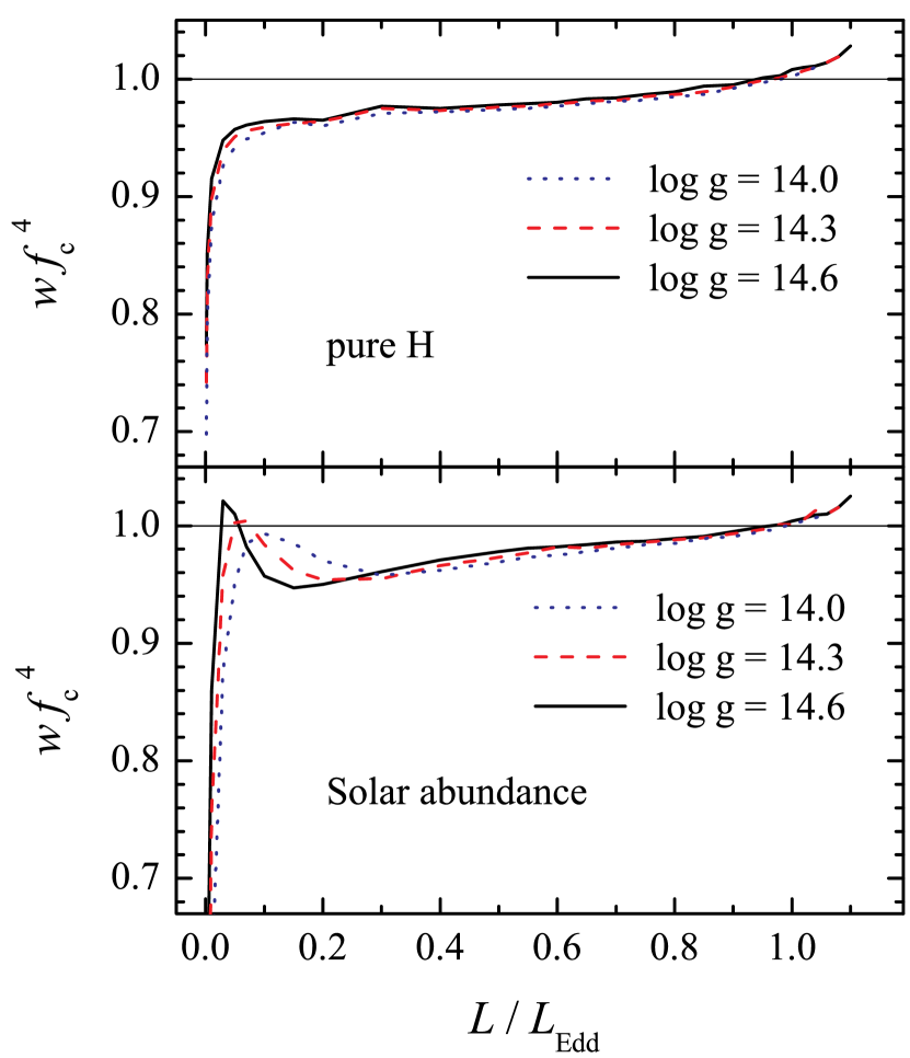
Figure 1: Dependence of the correction factor $wf_{\rm c}^{4}$ on the relative luminosity $\ell$ for various $\log g$ and two chemical compositions.

The actual spectra from the NS atmosphere models have been fitted in the energy band 3–20 keV (corresponding to the largest effective area of the Proportional Counter Array onboard of the Rossi X-ray Timing Explorer) with the two-parameter model (Suleimanov et al., 2011a, 2012; Nättilä et al., 2015)

$$\mathcal{F}_{\rm E}\approx w\pi B_{\rm E}(f_{\rm c}T_{\rm eff}),$$ (21)

allowing the spectral dilution factor $w$ to be different from $f_{\rm c}^{-4}$. The values $wf_{\rm c}^{4}$ were also tabulated. For the standard method, we used the presentation of the normalization (17), because the values $wf_{\rm c}^{4}$ are close to unity for almost all $\ell$ and the deviations become significant only at low luminosities, $\ell\lesssim 0.1$, which are unimportant for the cooling tail method (see Fig. 1).

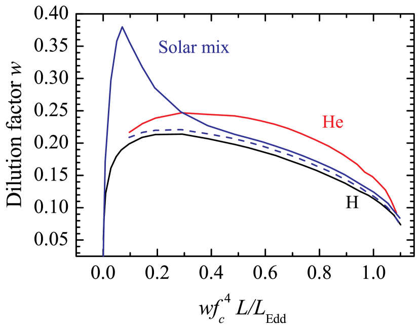
Figure 2: Dependences of the dilution factor $w$ on the model corrected relative luminosity $wf_{\rm c}^{4}\ell$ for fixed $\log g=14.3$ and various chemical compositions. The dashed curve corresponds to the solar H/He mix and reduced metal abundance ($Z=0.01Z_{\odot}$).

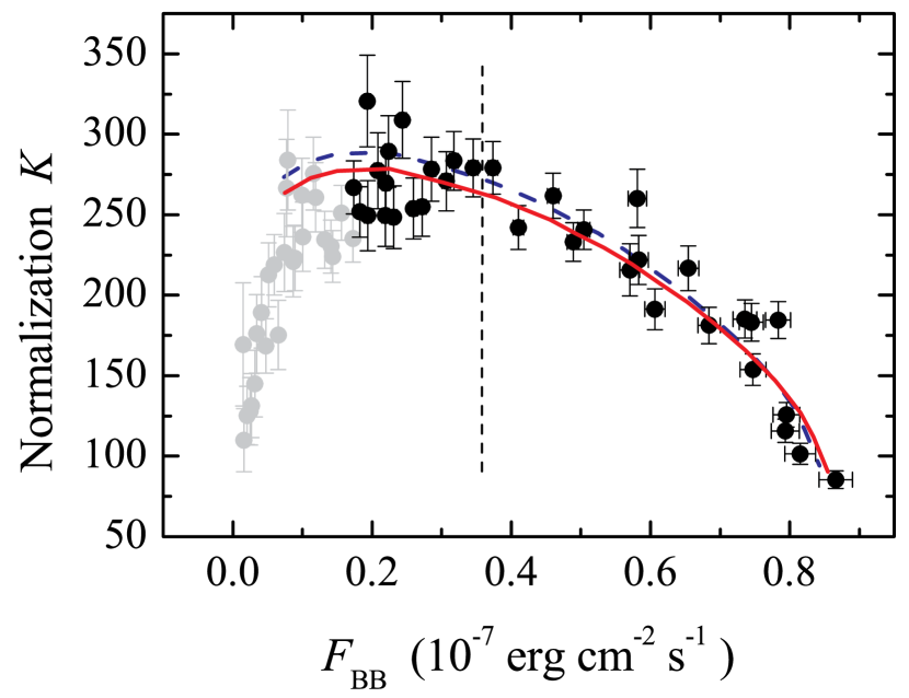
Figure 3: The observed $K-F_{\rm BB}$ dependence (circles with error bars) for the cooling tail (after touchdown) of the PRE burst of SAX J1810.8–2609 (see Nättilä et al., 2016). The red solid and the blue dashed curves are the best-fitting theoretical dependences $w-wf_{\rm c}^{4}\ell$ for solar H/He mix ($Z=0.01Z_{\odot}$) and $\log g=14.3$ corresponding to the data above $F_{\min}=0.2F_{\rm td}$ (black circles) and $F_{\min}=0.4F_{\rm td}$ (points to the right of the vertical dashed line), respectively. The best-fitting parameters are given in Table 1.

Let us now adjust the cooling tail method accounting for the correct spectral dilution factor. We note that the two parameter fitting (21) does not conserve the surface bolometric flux

$$\int_{0}^{\infty}w\pi B_{\rm E}(f_{\rm c}T_{\rm eff})\,dE=wf_{\rm c}^{4}\,\sigma_{\rm SB}T_{\rm eff}^{4},$$ (22)

and we need a bolometric correction factor $(wf_{\rm c}^{4})^{-1}$ to convert the observed blackbody flux to the actual bolometric flux

$$F_{\infty}=(wf_{\rm c}^{4})^{-1}\,F_{\rm BB}.$$ (23)

Thus, we can relate the observed black body flux to the relative luminosity as

$$F_{\rm BB}=(wf_{\rm c}^{4})\ l\ F_{\rm Edd}.$$ (24)

Therefore, the relation between the observed blackbody normalization $K$ and the NS radius, distance, and the spectral fitting parameters also changes:

$$(wf_{\rm c}^{4})^{-1}\,T_{\rm BB}^{4}\,K=T_{\infty}^{4}\,\Omega,$$ (25)

or

$$K=w\,\Omega.$$ (26)

Therefore, formally we have to fit the observed dependences $K^{-1/4}-F_{\rm BB}$ with the computed relations $w^{-1/4}-wf_{\rm c}^{4}\,\ell$, or simply just fitting the observed $K-F_{\rm BB}$ dependency by $w-wf_{\rm c}^{4}\,\ell$ (see equations 24 and 26 and Fig. 2). From here on, in order to simplify the presentation, we use the latter dependence.

There are two fitting parameters for this procedure, $F_{\rm Edd}$ and $\Omega$. They can be combined to get the observed Eddington temperature $T_{\rm Edd,\infty}$ given by equation (7):

$$T_{\rm Edd,\infty}=9.81\,\left(F_{\rm Edd,-7}/\Omega\mbox{[(km/10~{}kpc)}^{2}]\right)^{1/4}\,{\rm keV}.$$ (27)

The curves of equal $T_{\rm Edd,\infty}$ on the $M-R$ plane allow to limit the NS mass and radius. The second parameter, $\Omega$, could be useful if the distance is known, otherwise the distance can be estimated using its value.

To illustrate the method and demonstrate the differences between the new and the old approaches, we use the observational data of a PRE burst from SAX J1810.8–2609 analysed by Nättilä et al. (2016). We leave the analysis of other sources for the future. To allow an easy comparison with previous results, we select the data points after the touchdown down to the minimum flux $F_{\min}$ corresponding to 20 per cent of the touchdown flux $F_{\rm td}$ (see Fig. 3). To evaluate the effect of the data selection we also considered $F_{\min}=0.4F_{\rm td}$. The best-fitting solution was found with the simple Deming (2011) regression method by minimizing the function

$$\chi^{2}\!\!=\!\!\sum_{i=1}^{N_{\rm obs}}\left[\frac{(w\,\Omega-K_{i})^{2}}{\Delta K_{i}^{2}}+\frac{(wf_{\rm c}^{4}\,\ell\,F_{\rm Edd,-7}-F_{\rm BB,i})^{2}}{\Delta F_{\rm BB,i}^{2}}\right],$$ (28)

which takes into account errors on both axes. The term in the square brackets is the square of the minimal dimensionless distance from the given observed point to the model curve $w-wf_{\rm c}^{4}\,\ell$ with the given fitting parameters $\Omega$ and $F_{\rm Edd,-7}$. The curve of constant $T_{\rm Edd,\infty}$ corresponding to the best-fitting parameters for $\log g=$14.3 is shown in Fig. 4 by the solid red curve, while similar curve obtained with the standard cooling tail method (see Table 1 in Nättilä et al. 2016) is shown with the dotted red curve. It is clear that the new method gives NS radii larger by about 0.5 km. The reason is clear from equations (24) and (26). The inverse bolometric correction $wf_{\rm c}^{4}$ stretches the model curve, shifting it to higher fluxes at $\ell\gtrsim 0.9$ and to lower fluxes for $\ell\lesssim 0.9$ (see Fig. 1). In order to fit the data, we would need to decrease $F_{\rm Edd}$ and at the same time to increase $\Omega$. Both of these changes lead to smaller $T_{\rm Edd,\infty}$ and shift the corresponding solution to larger NS radii on the $M-R$ plane.

Table 1: Parameters of the fits of the $K-F_{\rm BB}$ dependency with the corrected cooling tail models for various $\log g$.

$\log g$	$F_{\rm Edd}$	$\Omega$	$T_{\rm Edd,\infty}$	$\chi^{2}$/dof
	$10^{-7}$ erg cm-2 s-1	(km/10 kpc)2	(keV)
$F_{\min}=0.2F_{\rm td}$
14.6	0.771	1222	1.555	58.6/33
14.3	0.776	1261	1.545	45.8/33
14.0	0.776	1315	1.529	44.5/33
$F_{\min}=0.4F_{\rm td}$
14.6	0.753	1293	1.524	30.6/17
14.3	0.765	1308	1.525	28.8/17
14.0	0.771	1338	1.520	27.8/17

The computed curves $f_{\rm c}-\ell$ (as well as the curves $w-wf_{\rm c}^{4}\,\ell$) are slightly different for different $\log g$ (Suleimanov et al., 2011a, 2012; Nättilä et al., 2015). Therefore, if we fit the observed curve $K-F_{\rm BB}$ with the theoretical dependences computed for different $\log g$, we will obtain slightly different fitting parameters $\Omega$ and $F_{\rm Edd,-7}$. As a result, the observed Eddington temperature $T_{\rm Edd,\infty}$ will be also different together with corresponding curves at the $M-R$ plane (see Fig. 4 and Table 1). In fact, the constant $T_{\rm Edd,\infty}$ curves corresponding to different $\log g$ give correct values of NS $M$ and $R$ only at the crossing points with the corresponding constant $\log g$ curves. Fortunately, all constant $T_{\rm Edd,\infty}$ curves are close to each other within the statistical uncertainties.

We note here that the solution depends slightly on the number of data points used in the fits and the method to find the best-fitting solution. For example, if we take the points above $F_{\min}=0.4F_{\rm td}$, the constant $T_{\rm Edd,\infty}$ curve corresponding to the best-fitting $\chi^{2}$ solution shifts to larger NS radii (dashed red curve in Fig. 4 and Table 1).

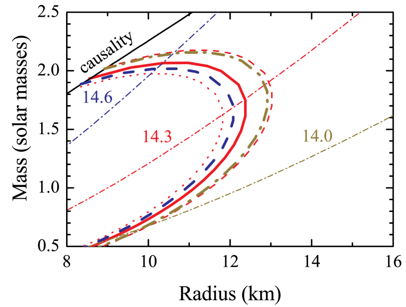
Figure 4: Curves of constant $T_{\rm Edd,\infty}$ on the $M-R$ plane, obtained from the data with $F_{\min}=0.2F_{\rm td}$ and three different $\log g=$14.6 (dashed blue curve), 14.3 (solid red curve), and 14.0 (dot-dashed brown curve). The best fit parameters are given in Table 1. The red thin dotted curve corresponds to the best-fitting $T_{\rm Edd,\infty}$ from Nättilä et al. (2016) for the same data. The red thin dashed curve corresponds to $F_{\min}=0.4F_{\rm td}$ and $\log g=14.3$. The constant $\log g$ curves are shown by the thin dot-dashed lines.

3 Direct cooling tail method

Formally, the cooling tail method gives a correct result only at the crossing point of the curves of the constant $\log g$ and the corresponding $T_{\rm Edd,\infty}$. Therefore, we suggest here a direct cooling tail method with $M$ and $R$ as fitting parameters. This method is free from the weakness of the standard method (see also Özel & Psaltis, 2015, for more discussion) and allows us to obtain solutions at the $R=2R_{\rm S}$ line as well. Moreover, the new formalism gives a possibility to take into account different priors in the physical parameters $M$ and $R$, and, for example, to control the minimum (or maximum) allowed mass in the fit.

For every pair $M$ and $R$ we can compute the gravity $\log g$, surface gravitational redshift $z$, and (assuming some chemical composition) the observed Eddington temperature $T_{\rm Edd,\infty}$ (see equations (1), (3), and (27)). We use interpolation in the sets of $f_{\rm c}-\ell$ and $wf_{\rm c}^{4}-\ell$ curves, computed for different values of $\log g$, for finding the theoretical curve $w-wf_{\rm c}^{4}\,\ell$ corresponding to a given $\log g$.

3.1 Method of interpolation

To improve the accuracy of the interpolation, we have extended the existing set of hot NS model atmospheres for $\log g$ = 14.0, 14.3, and 14.6 (Suleimanov et al., 2012) to values from 13.7 up to 14.9 with the step 0.15 (i.e. nine values). We use the same relative luminosity set $\ell$ as in the previous work of Suleimanov et al. (2012), but for $\ell\geq 0.1$ only. Such computations were performed for four chemical compositions, pure hydrogen, pure helium, and solar H/He mix with solar ($Z=Z_{\odot}$) and sub-solar ($Z=0.01Z_{\odot}$) metal abundances. The model emergent spectra were fitted with a diluted blackbody (see details in Suleimanov et al. 2011a) and corresponding values of $f_{\rm c}$, $wf_{\rm c}^{4}$, and of the radiative acceleration $g_{\rm rad}$ were obtained.

Spectral fit parameters $f_{\rm c}$ and $w$ depend on the relative luminosity $\ell$ in a similar way at different $\log g$, when $\ell$ is small enough ($\ell<0.8$). But significant differences arise at larger $\ell$ because real electron scattering opacity decreases when the plasma temperature increases (see Suleimanov et al. 2012). As a result, the maximum possible luminosity relative to the Eddington luminosity for Thomson opacity, $\ell$, also increases. Therefore, it is natural to use dependences of the type $f_{\rm c}-g_{\rm rad}/g$ for interpolation, which are similar to each other for all surface gravities (see Fig. 8 in Suleimanov et al. 2012). At the first step, we find $g_{\rm rad}/g$ values corresponding to the $\ell$ grid. Then we introduce the fixed grid of $g_{\rm rad}/g$ and interpolate all the necessary parameters ($T_{\rm eff}$, $f_{\rm c}$, and $w$), to the new grid $g_{\rm rad}/g$ at every $\log g$. At the final step, we get the theoretical dependence $w-wf_{\rm c}^{4}\,\ell$ for the $\log g$ computed for the investigated $M$ and $R$ pair by interpolating all the quantities on the grid of nine values of $\log g$. In this work we use the interpolation along weighting backward and forward parabolas (see detail in Kurucz, 1970).

3.2 Fitting procedure

For the corrected cooling tail method we can use two fitting parameters, $\Omega$ and $F_{\rm Edd,-7}$. However, for a given $M$ and $R$ pair, $L_{\rm Edd}$ is already determined by their values, and both fitting parameters depend on only one parameter – the distance to the source $D$. This allows us to obtain an estimation of the distance to the source given the chemical composition of the NS atmosphere and to limit the final solution if there exist independent constraints on the distance.

In the direct cooling tail method, we minimize $\chi^{2}$ at a grid in the $M-R$ plane by fitting the observed $K-F_{\rm BB}$ curve with the theoretical $w-wf_{\rm c}^{4}\,\ell$ curve interpolated to the current $\log g$ using $D_{10}$ as the only fitting parameter. We consider a grid of masses from 1 to 3${\rm M}_{\odot}$ with the step 0.01${\rm M}_{\odot}$ and a grid of radii from 9 to 17 km with the step 0.01 km. We ignore the pairs which do not satisfy the causality condition $R>1.45R_{\rm S}$ (Lattimer & Prakash, 2007). We thus obtain the map of best-fitting $D$ and the $\chi^{2}$ values at the $M-R$ plane and the overall minimum of $\chi^{2}$, which allow us to find the confidence regions (e.g. for two parameters, $\Delta\chi^{2}=2.3,4.61,9.21$ give probabilities of 68, 90 and 99%). We note here that, the method used for finding the best-fitting solution, e.g. the $\chi^{2}$-method like here and in Suleimanov et al. (2011b), or the robust likelihood method from Poutanen et al. (2014), affects only slightly (within the 1$\sigma$ error) the centroid of the solution. On the other hand, the resulting error contours on the $M-R$ plane are affected more: the $\chi^{2}$-method generally underestimates the errors, because of the presence of the significant scattering in the data as well as because the best-fitting solution may be located at the boundary of the prior distributions. The robust estimator gives more correct presentation of the errors when benchmarked against a full Bayesian fit with intrinsic scatter in the system. For simplicity we, however, here show only the results obtained by minimizing a non-robust $\chi^{2}$ function given by equation (28).

We apply the direct cooling tail method to the data described above and presented in Fig. 3. The minimum $\chi^{2}$ is 45.4 for 32 dof. The confidence regions at the $M-R$ plane are shown in Fig. 5. To compare with the results presented in Fig. 4 we also draw the curve of equal $T_{\rm Edd,\infty}$ obtained using the corrected cooling tail method for $\log g$= 14.3 (red solid curve). There is good correspondence between this curve and the confidence regions given by the direct method. To compare with the previous result, the curve of equal $T_{\rm Edd,\infty}$ obtained with the standard cooling tail method (Table 2 in Nättilä et al., 2016) is also shown (red dotted curve). We remind here that the method does not suffer from the problems with the Jacobian transformation from $F_{\rm Edd},\Omega$ to $M,R$ (see discussion in Özel & Psaltis, 2015), because we fit directly on the $M-R$ plane. We also see that instead of the two regions of allowed solutions (small $R$, large $M$ and large $R$, smaller $M$; see e.g. Suleimanov et al. 2011b; Poutanen et al. 2014) the solution here prefers larger $R$ and smaller $M$ values. This is a direct consequence of the fact that the shape of the $w-wf_{\rm c}^{4}\,\ell$ curves depends on $\log g$ and a smaller $\log g$ gives a better description of the data (see Table 1).

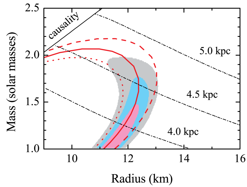
Figure 5: The $\chi^{2}$ confidence regions (68, 90 and 99% probabilities) in the mass-radius plane for SAX J1810.8–2609 obtained using the direct cooling tail method. The data above $F_{\min}=0.2F_{\rm td}$ (see Fig. 3) are used. The red solid and dashed curves correspond to the best-fitting $T_{\rm Edd,\infty}$ obtained for $\log g$=14.3 for $F_{\min}=0.2F_{\rm td}$ and $0.4F_{\rm td}$, respectively, while the red dotted curve gives the results from Nättilä et al. (2016). The black dot-dashed curves correspond to the constant distance of 4.0, 4.5, and 5.0 kpc.

We conclude that the most probable radius of the NS in SAX J1810.8–2609 lies in the range between 11.5 and 13.0 km for the mass range of 1.3–1.8${\rm M}_{\odot}$. However, the smaller radii of $\sim$10 km for a high-mass ($\sim 2{\rm M}_{\odot}$) NS cannot be formally excluded. The obtained constraints also limit the possible distance to the source, which likely lies in the interval between 3.7 and 4.7 kpc.

4 Summary

We have presented the direct cooling tail method, which takes NS mass and radius together with the distance as the direct fitting parameters. This method implies fitting of an observed dependence between blackbody fitting parameters, the normalization and the observed blackbody flux, $K-F_{\rm BB}$, with the corresponding theoretical dependence, $w-wf_{\rm c}^{4}\,\ell$, which is found for every given $M$ and $R$ pair by interpolation in the extended grid (for nine values of $\log g$) of the computed dependences $f_{\rm c}-\ell$ and $wf_{\rm c}^{4}-\ell$. Such grids were computed for 4 chemical compositions: pure H and pure He, and solar H/He mix with the solar ($Z=Z_{\odot}$) and sub-solar ($Z=0.01Z_{\odot}$) metal abundances. The fitting procedure results in the $\chi^{2}$ maps and corresponding confidence regions in the $M-R$ plane. Other fitting methods (robust likelihood, Bayesian) give very similar results with slightly larger errors. Compared with the standard cooling tail method, the new method does not suffer from the problems with the Jacobian transformation from $(F_{\rm Edd},\Omega)$ to $(M,R)$ allowing to obtain solution anywhere on the $M-R$ plane.

We applied the new method to a PRE burst that occurred in the low/hard state of SAX J1810.8–2609. The direct cooling tail method gives the Eddington temperature slightly smaller than the standard cooling tail method, resulting in a systematic shift of the radii by $\sim 1\,\sigma$ to larger values (which is still within the statistical uncertainties). However, instead of the two separated $(M,R)$ regions usually obtained with the standard method, our solution prefers larger $R$ and smaller $M$ values corresponding to smaller $\log g$ values, which is a direct consequence of the dependence of the theoretical cooling curves $w-wf_{\rm c}^{4}\,\ell$ on gravity. We finally constrain the NS radius in SAX J1810.8–2609 to lie between 11.5 and 13.0 km for the assumed mass range of 1.3–1.8${\rm M}_{\odot}$. The distance to the source likely lies between 3.7 and 4.7 kpc.

References

- Antoniadis et al. (2013) Antoniadis J., et al., 2013, Science, 340, 448
- Damen et al. (1990) Damen E., Magnier E., Lewin W. H. G., Tan J., Penninx W., van Paradijs J., 1990, A&A, 237, 103
- Deming (2011) Deming W. E., 2011, Statistical Adjustment of Data (Dover Books on Mathematics). Dover Publications, New York
- Ebisuzaki (1987) Ebisuzaki T., 1987, PASJ, 39, 287
- Galloway et al. (2008) Galloway D. K., Muno M. P., Hartman J. M., Psaltis D., Chakrabarty D., 2008, ApJS, 179, 360
- Guillot et al. (2013) Guillot S., Servillat M., Webb N. A., Rutledge R. E., 2013, ApJ, 772, 7
- Güver et al. (2012) Güver T., Psaltis D., Özel F., 2012, ApJ, 747, 76
- Haensel et al. (2007) Haensel P., Potekhin A. Y., Yakovlev D. G., 2007, Neutron Stars 1: Equation of State and Structure. Astrophysics and Space Science Library Vol. 326, Springer, New York
- Heinke et al. (2006) Heinke C. O., Rybicki G. B., Narayan R., Grindlay J. E., 2006, ApJ, 644, 1090
- Heinke et al. (2014) Heinke C. O., et al., 2014, MNRAS, 444, 443
- Ho & Heinke (2009) Ho W. C. G., Heinke C. O., 2009, Nature, 462, 71
- Kajava et al. (2014) Kajava J. J. E., et al., 2014, MNRAS, 445, 4218
- Kajava et al. (2017) Kajava J. J. E., Nättilä J., Poutanen J., Cumming A., Suleimanov V., Kuulkers E., 2017, MNRAS, 464, L6
- Kiziltan et al. (2013) Kiziltan B., Kottas A., De Yoreo M., Thorsett S. E., 2013, ApJ, 778, 66
- Klochkov et al. (2013) Klochkov D., Pühlhofer G., Suleimanov V., Simon S., Werner K., Santangelo A., 2013, A&A, 556, A41
- Klochkov et al. (2015) Klochkov D., Suleimanov V., Pühlhofer G., Yakovlev D. G., Santangelo A., Werner K., 2015, A&A, 573, A53
- Koljonen et al. (2016) Koljonen K. I. I., Kajava J. J. E., Kuulkers E., 2016, ApJ, 829, 91
- Kramer & Wex (2009) Kramer M., Wex N., 2009, Classical and Quantum Gravity, 26, 073001
- Kurucz (1970) Kurucz R. L., 1970, SAO Special Report, 309
- Kuśmierek et al. (2011) Kuśmierek K., Madej J., Kuulkers E., 2011, MNRAS, 415, 3344
- Lattimer & Prakash (2007) Lattimer J. M., Prakash M., 2007, Phys. Rep., 442, 109
- Lattimer & Steiner (2014) Lattimer J. M., Steiner A. W., 2014, ApJ, 784, 123
- Lewin et al. (1993) Lewin W. H. G., van Paradijs J., Taam R. E., 1993, Space Science Reviews, 62, 223
- Lo et al. (2013) Lo K. H., Miller M. C., Bhattacharyya S., Lamb F. K., 2013, ApJ, 776, 19
- Miller (2013) Miller M. C., 2013, preprint, (arXiv:1312.0029)
- Miller & Lamb (2015) Miller M. C., Lamb F. K., 2015, ApJ, 808, 31
- Miller & Lamb (2016) Miller M. C., Lamb F. K., 2016, European Physical Journal A, 52, 63
- Nättilä et al. (2015) Nättilä J., Suleimanov V. F., Kajava J. J. E., Poutanen J., 2015, A&A, 581, A83
- Nättilä et al. (2016) Nättilä J., Steiner A. W., Kajava J. J. E., Suleimanov V. F., Poutanen J., 2016, A&A, 591, A25
- Özel (2006) Özel F., 2006, Nature, 441, 1115
- Özel (2013) Özel F., 2013, Reports on Progress in Physics, 76, 016901
- Özel & Psaltis (2015) Özel F., Psaltis D., 2015, ApJ, 810, 135
- Özel et al. (2009) Özel F., Güver T., Psaltis D., 2009, ApJ, 693, 1775
- Özel et al. (2012) Özel F., Psaltis D., Narayan R., Santos Villarreal A., 2012, ApJ, 757, 55
- Özel et al. (2016) Özel F., Psaltis D., Güver T., Baym G., Heinke C., Guillot S., 2016, ApJ, 820, 28
- Pavlov & Luna (2009) Pavlov G. G., Luna G. J. M., 2009, ApJ, 703, 910
- Poutanen & Gierliński (2003) Poutanen J., Gierliński M., 2003, MNRAS, 343, 1301
- Poutanen et al. (2014) Poutanen J., Nättilä J., Kajava J. J. E., Latvala O.-M., Galloway D. K., Kuulkers E., Suleimanov V. F., 2014, MNRAS, 442, 3777
- Steiner et al. (2010) Steiner A. W., Lattimer J. M., Brown E. F., 2010, ApJ, 722, 33
- Suleimanov & Werner (2007) Suleimanov V., Werner K., 2007, A&A, 466, 661
- Suleimanov et al. (2011a) Suleimanov V., Poutanen J., Werner K., 2011a, A&A, 527, A139
- Suleimanov et al. (2011b) Suleimanov V., Poutanen J., Revnivtsev M., Werner K., 2011b, ApJ, 742, 122
- Suleimanov et al. (2012) Suleimanov V., Poutanen J., Werner K., 2012, A&A, 545, A120
- Suleimanov et al. (2016) Suleimanov V. F., Poutanen J., Klochkov D., Werner K., 2016, European Physical Journal A, 52, 20
- Thorsett & Chakrabarty (1999) Thorsett S. E., Chakrabarty D., 1999, ApJ, 512, 288
- Watts et al. (2016) Watts A. L., et al., 2016, Reviews of Modern Physics, 88, 021001
- Worpel et al. (2015) Worpel H., Galloway D. K., Price D. J., 2015, ApJ, 801, 60
- Zavlin et al. (1996) Zavlin V. E., Pavlov G. G., Shibanov Y. A., 1996, A&A, 315, 141
- Zavlin et al. (1998) Zavlin V. E., Pavlov G. G., Trumper J., 1998, A&A, 331, 821
- van Paradijs et al. (1990) van Paradijs J., Dotani T., Tanaka Y., Tsuru T., 1990, PASJ, 42, 633