Revisiting radiative decays of $1^{+-}$ heavy quarkonia in the covariant light-front approach

Abstract

We revisit the calculation of the width for the radiative decay of a $1^{+-}$ heavy $Q\bar{Q}$ meson via the channel $1^{+-}\to 0^{-+}+\gamma$ in the covariant light-front quark model. We carry out the reduction of the light-front amplitude in the non-relativistic limit, explicitly computing the leading and next-to-leading order relativistic corrections. This shows the consistency of the light-front approach with the non-relativistic formula for this electric dipole transition. Furthermore, the theoretical uncertainty in the predicted width is studied as a function of the inputs for the heavy quark mass and wavefunction structure parameter. We analyze the specific decays $h_{c}(1P)\to\eta_{c}(1S)+\gamma$ and $h_{b}(1P)\to\eta_{b}(1S)+\gamma$. We compare our results with experimental data and with other theoretical predictions from calculations based on non-relativistic models and their extensions to include relativistic effects, finding reasonable agreement.

I Introduction

Heavy-quark $Q\bar{Q}$ bound states play a valuable role in elucidating the properties of quantum chromodynamics (QCD). Since the discoveries of the $J/\psi$ in 1974 Aubert:1974js ; psi_slac and other $c\bar{c}$ charmonium states, and the $\Upsilon$ in 1977 Herb:1977ek ; Innes:1977ae and other $b\bar{b}$ states, we now have a very substantial set of data on the properties and decays of these quarkonium states. Some reviews include quiggrosner79 -rosner2013 . The goal of understanding these data motivates theoretical studies, in particular, studies of the decays of $Q\bar{Q}$ states.

Among various decay channels, radiative decays are a very good testing ground for models, since the emitted photon is directly detected and the electromagnetic interaction is well understood. An electric dipole (E1) transition is one the simplest types of radiative decays. Here we consider E1 transitions of the form

$${}^{1}P_{1}\to{}^{1}S_{0}+\gamma,$$ (1)

where a spin-singlet P-wave $Q\bar{Q}$ quarkonium state decays to a spin-singlet S-wave $Q\bar{Q}$ state. In terms of the spin $J$ and the charge and parity quantum numbers P and C, indicated as $J^{PC}$, this has the form $1^{+-}\to 0^{-+}+\gamma$.

Several theoretical analyses of these E1 transition rates have been carried out, using various models Karl:1980wm -Li:2009zu . A number of these models utilize the non-relativistic quantum mechanics formula for an E1 transition, involving the calculation of the overlap integral of the quarkonium wavefunctions of the initial and final states. The quarkonium wavefunction is obtained from the solution of the Schrödinger equation with non-relativistic potentials, such as the Cornell potential, $V=-(4/3)\alpha_{s}(m_{Q})/r+\sigma r$. The first term in this potential is a non-Abelian Coulomb potential representing one-gluon exchange at short distances, where $\alpha_{s}(m_{Q})=g_{s}(\mu)^{2}/(4\pi)$ is the strong coupling evaluated at the scale of the heavy quark mass, $m_{Q}$, and the second term is the linear confining potential, where $\sigma=0.18$ GeV² is the string tension. Current data yield a fit to $\alpha_{s}(\mu)$ such that $\alpha_{s}\simeq 0.33$ at the scale $\mu=1.5$ GeV relevant for $c\bar{c}$ states and $\alpha_{s}\simeq 0.21$ at the scale $\mu=4.7$ GeV relevant for $b\bar{b}$ states PDG . Relativistic corrections have also been calculated by replacing the Schrödinger equation by the Dirac equation, and computing corrections in powers of $v/c$, where $v$ is the velocity of the heavy (anti)quark in the rest frame of the $Q\bar{Q}$ bound state.

It is of interest to study the radiative decays (1) with a fully relativistic approach, namely the light-front quark model (LFQM)Terentev:1976jk -Cheng:2003sm . This approach naturally includes relativistic effects of quark spins and the internal motion of the constituent quarks. Another advantage of the light-front quark model is that it is manifestly covariant. Hence it is easy to boost a hadron bound state from one inertial Lorentz frame to another one when the bound state wavefunction is known in a particular frameBrodsky:1997de . The light-front approach has been used to study semileptonic and nonleptonic decays of heavy-flavor $D$ and $B$ mesons and also to evaluate radiative decay rates of heavy mesons Hwang:2006cua ; Choi:2007se ; Hwang:2010iq ; Ke:2010vn ; Ke:2013zs ; Shi:2016nxr .

In this paper, we extend our previous work with Ke and Li in Ref.Ke:2013zs on the study of the radiative decays

$$h_{c}(1P)\to\eta_{c}(1S)+\gamma\ ,$$ (2)

and

$$h_{b}(1P)\to\eta_{b}(1S)+\gamma\ .$$ (3)

We present several new results here. We carry out the reduction of the light-front amplitude to the non-relativistic limit, explicitly computing the leading and next-to-leading order relativistic corrections. This shows the consistency of the light-front approach with the non-relativistic formula for this electric dipole transition. Furthermore, we investigate the theoretical uncertainties in the predicted widths as functions of the inputs for the heavy quark mass and wavefunction structure parameters. As in Ref. Ke:2013zs , we compare our numerical results for these widths with experimental data and with other theoretical predictions from calculations based on non-relativistic models and their extensions to include relativistic effects, extending Ke:2013zs with further study of the theoretical uncertainties in our calculations. Specifically, we compare our numerical results with results from Voloshin:2007dx ; Brambilla:2004wf ; Ebert:2002pp ; Li:2009nr ; Godfrey:2015dia ; Segovia:2016xqb ; Barnes:2005pb ; Li:2009zu as well as latest experimental data PDG .

The paper is organized as follows: In Section II, we review the formulas for the radiative decay $1^{+-}\to 1^{-+}+\gamma$. In section III, we analyze the reduction of light-front formulas when applied to heavy quarkonium systems to non-relativistic limit and compare these with non-relativistic quantum mechanical electric dipole transition formula. In Section IV, we present our numerical results for the decay widths of $h_{c}(1P)\to\eta_{c}(1S)+\gamma$ and $h_{b}(1P)\to\eta_{b}(1S)+\gamma$ including an extended analysis of the theoretical uncertainties. Our conclusions are given in Section V.

II Light-front formalism for the decays $1^{+-}\to 0^{-+}+\gamma$

II.1 Notation

We first define some notation, retaining the conventions of Jaus:1999zv ; Cheng:2003sm . In light-front coordinates, the four-momentum $p$ is

$$p^{\mu}=(p^{-},p^{+},{\bf p}_{\perp})$$ (4)

where $p^{\pm}=p^{0}\pm p^{3}$ and ${\bf p}_{\perp}=(p^{1},p^{2})$. Hence, the Lorentz scalar product $p^{2}=p_{\mu}p^{\mu}$ is

$$p^{2} = (p^{0})^{2}-|{\bf p}|^{2}=(p^{0})^{2}-(p^{3})^{2}-|{\bf p}_{\perp}|^{2}$$ (5)

$$= p^{+}p^{-}-|{\bf p}_{\perp}|^{2}\ .$$ (7)

Consider a decay of a $Q\bar{Q}$ meson consisting of two constituent particles (quark and antiquark). The momentum of the parent meson is denoted as $P^{\prime}=p^{\prime}_{1}+p_{2}$, where $p^{\prime}_{1}$ and $p_{2}$ are the momenta of the constituent quark and antiquark, with mass $m^{\prime}_{1}$ and $m_{2}$, respectively. The momentum of the daughter $Q\bar{Q}$ meson is written as $P^{\prime\prime}=p^{\prime\prime}_{1}+p_{2}$, where $p^{\prime\prime}_{1}$ is the momentum of the constituent quark, with mass $m^{\prime\prime}_{1}$. Here we have $m^{\prime}_{1}=m_{2}=m^{\prime\prime}=m_{Q}$. The four-momentum of the parent meson with mass $M^{\prime}$ can be expressed as $P^{\prime}=(P^{\prime-},P^{\prime+},{\bf P}^{\prime}_{\perp})$, where $P^{\prime 2}=P^{\prime+}P^{\prime-}-|{\bf P^{\prime}}_{\perp}|^{2}=M^{\prime 2}$. Similarly, for the daughter meson with mass $M^{\prime\prime}$, one has $P^{\prime\prime 2}=M^{\prime\prime 2}$, as shown in Fig. 1 below. (Vector signs on transverse momentum components are henceforth taken to be implicit.)

The momenta of the constituent quark and antiquark ($p^{\prime}_{1}$, $p^{\prime\prime}_{1}$ and $p_{2}$) can be described by internal variables $(x_{2},p^{\prime}_{\perp})$ thus:

$$p^{\prime+}_{1}=x_{1}P^{\prime+},\quad p^{+}_{2}=x_{2}P^{\prime+}$$

$$p^{\prime}_{1\perp}=x_{1}P^{\prime}_{\perp}+p^{\prime}_{\perp},\quad p_{2\perp}=x_{2}P^{\prime}_{\perp}-p^{\prime}_{\perp}$$

$$x_{1}+x_{2}=1\ .$$ (8)

Explicitly,

$$x_{1}=\frac{e_{1}-p^{\prime}_{z}}{e^{\prime}_{1}+e_{2}}\ ,\quad x_{2}=\frac{p^{\prime}_{z}+e_{2}}{e^{\prime}_{1}+e_{2}}\ ,$$ (9)

where $e^{\prime}_{1}$, $e^{\prime\prime}_{1}$ and $e_{2}$ are the energy of the quark (anti-quark) with momenta $p^{\prime}_{1}$, $p^{\prime\prime}_{1}$ and $p_{2}$:

$$e^{\prime}_{1} = \sqrt{m^{\prime 2}_{1}+p^{\prime 2}_{\perp}+p^{\prime 2}_{z}}$$

$$e^{\prime\prime}_{1} = \sqrt{m^{\prime\prime 2}_{1}+p^{\prime\prime 2}_{\perp}+p^{\prime\prime 2}_{z}}$$

$$e_{2} = \sqrt{m^{2}_{2}+p^{\prime 2}_{\perp}+p^{\prime 2}_{z}}\ .$$ (10)

With the external momentum of the photon given as $q=P^{\prime}-P^{\prime\prime}$, $p^{\prime\prime}_{\perp}$ can be expressed as

$$p^{\prime\prime}_{\perp}=p^{\prime}_{\perp}-x_{2}q_{\perp}.$$ (11)

Here $p^{\prime}_{z}$ and $p^{\prime\prime}_{z}$ can also be expressed as functions of internal variables $(x_{2},p^{\prime}_{\perp})$, and explicit expressions can be found in Appendix B.

II.2 Form factors

Define external momentum variables to be $P=P^{\prime}+P^{\prime\prime}$, $q=P^{\prime}-P^{\prime\prime}$, where $q$ is the four-momentum of the photon that is emitted in the radiative transition. The general amplitude of the radiative decay (1) of the axial vector $1^{+-}$ ${}^{1}P_{1}$ meson, denoted as $A$, to the pseudoscalar $0^{-+}$ ${}^{1}S_{0}$ meson, denoted as $P$, can be written as Cheng:2003sm :

$$i{\cal A}\left(A(P^{\prime})\to P(P^{\prime\prime})\gamma(q)\right)=\varepsilon^{*}_{\mu}(q)\varepsilon^{\prime}_{\nu}(P^{\prime})i\tilde{\cal A}^{\mu\nu}\ ,$$ (12)

where

$$i\tilde{\cal A}^{\mu\nu}=f_{1}(q^{2})g^{\mu\nu}+P^{\mu}\left[f_{+}(q^{2})P^{\nu}+f_{-}(q^{2})q^{\nu}\right]\ .$$ (13)

In the above expression, we have used the condition $\varepsilon^{*}_{\mu}(q)q^{\mu}=0$ to eliminate terms that are proportional to $q^{\mu}$. This expression can be simplified further by using the transversality property of axial vector polarization vector:

$$\varepsilon^{\prime}_{\nu}(P^{\prime})(P+q)^{\nu}=0\ .$$ (14)

Then the general amplitude can be written as

$$i\tilde{\cal A}^{\mu\nu}\to i{\cal A}^{\mu\nu}=f_{1}(q^{2})g^{\mu\nu}+f_{2}(q^{2})P^{\mu}q^{\nu}\ ,$$ (15)

where $f_{2}(q^{2})$ is linear combination of $f_{+}(q^{2})$ and $f_{-}(q^{2})$:

$$f_{2}(q^{2})=-f_{+}(q^{2})+f_{-}(q^{2})\ .$$ (16)

Notice that in Eq.(15), $f_{1}(q^{2})$ and $f_{2}(q^{2})$ are not independent. Because of electromagnetic gauge invariance, they are related by the following equation:

$$q_{\mu}{\cal A}^{\mu\nu}=0\ \to\ f_{1}(q^{2})+f_{2}(q^{2})(P\cdot q)=0\ .$$ (17)

We find that the $f_{2}(q^{2})$ term in the amplitude (Eq.(15)) does not contribute to the width, due to the fact that the photon has only two transverse polarization states, so that the timelike component $\varepsilon^{*}_{0}(q)$ is equal to zero. Taking the parent axial vector meson $A(P^{\prime})$ in its rest frame, we have $P^{\prime}_{\nu}=(M^{\prime},0)$, where $M^{\prime}$ is the mass of the vector meson $A(P^{\prime})$. The contribution of the $f_{2}(q^{2})$ term is zero after we contract ${\cal A}^{\mu\nu}$ with polarization vector $\varepsilon^{*}_{\mu}(q)$:

$$\varepsilon^{*}_{\mu}(q)\varepsilon^{\prime}_{\nu}(P^{\prime})[f_{2}(q^{2})P^{\mu}q^{\nu}]\propto\varepsilon^{*}_{\mu}(q)P^{\prime\mu}=\varepsilon^{*}_{0}(q)P^{\prime 0}=0\ .$$ (18)

That fact that $f_{2}(q^{2})$ has no contribution can also be shown straightforwardly when we calculate the transition probability $|{\cal A}|^{2}$, using exact summation of two physical polarizations of photon:

$$\sum\varepsilon^{*}_{\mu}(q)\varepsilon_{\alpha}(q)=-g_{\mu\alpha}+\frac{q_{\mu}\eta_{\alpha}+q_{\alpha}\eta_{\mu}}{2q\cdot\eta}\ ,$$ (19)

where $q=(|{\bf q}|,{\bf q})$ and $\eta=(|{\bf q}|,-{\bf q})$. After an explicit calculation, we have

$$\sum_{\text{ polarization}}|{\cal A}|^{2}=2|f_{1}(q^{2})|^{2}\ .$$ (20)

Taking the physical value $q^{2}\to 0$ in the form factor $f_{1}(q^{2})$ and averaging initial state polarizations, the radiative transition width of $1^{+-}\to 0^{-+}+\gamma$ is given by

$$\Gamma=\frac{1}{3}\cdot\frac{|{\bf q}|}{8\pi M^{\prime 2}}\sum_{\text{polar.}}|{\cal A}|^{2}=\frac{|\bf{q}|}{12\pi M^{\prime 2}}\cdot|f_{1}(0)|^{2}\ ,$$ (21)

where the energy of the emitted photon is related to the masses of mesons as $|{\bf q}|=(M^{\prime 2}-M^{\prime\prime 2})/(2M^{\prime})$.

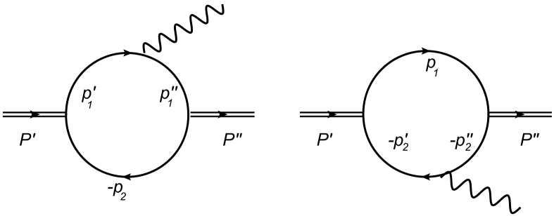
Figure 1: Feynman diagrams for radiative transition $1^{+-}\to 0^{-+}+\gamma$ in the light-front approach.

II.3 Calculation of radiative decay amplitude

In the covariant light-front quark model, the vertex function of the axial vector meson $A$ ($1^{+-}$,${}^{1}P_{1}$) is given by

$$-iH^{\prime}_{A}\left[\frac{1}{W^{\prime}_{A}}(p^{\prime}_{1}-p_{2})^{\mu}\right]\gamma^{5}\ ,$$ (22)

and the vertex function of the pseudoscalar meson $P$ ($0^{-+}$,${}^{1}S_{0}$) is given by

$$H^{\prime\prime}_{P}\gamma^{5}\ ,$$ (23)

where $H^{\prime}_{A}$ and $H^{\prime\prime}_{P}$ are functions of $p^{\prime}_{1}$ and $p_{2}$, and $W^{\prime}_{A}$ can be reduced to a constant, which we will discuss later in this subsection.

In the light-front framework that we use Jaus:1999zv ; Cheng:2003sm , at leading order there are two diagrams that contribute to the $A\to P+\gamma$ transition amplitude. These give the corresponding contributions to this amplitude

$$i{\cal A}^{\mu\nu}(A\to P+\gamma)=i{\cal A}^{\mu\nu}(a)+i{\cal A}^{\mu\nu}(b)$$ (24)

where $i{\cal A}^{\mu\nu}(a)$ and $i{\cal A}^{\mu\nu}(b)$ correspond to the left and right diagram in Fig.(1), respectively. The contribution to the amplitude from the right diagram can be obtained by taking the charge conjugation of left diagram (see also Shi:2016nxr ). So we discuss the left-hand diagram, where the corresponding transition amplitude is given by

$$i{\cal A}^{\mu\nu}(a)=i\frac{eN_{e^{\prime}_{1}}N_{c}}{(2\pi)^{4}}\int d^{4}p^{\prime}_{1}\,\frac{H^{\prime}_{A}H^{\prime\prime}_{P}}{N^{\prime}_{1}N^{\prime\prime}_{1}N_{2}}{\cal S}^{\mu\nu}_{a}\ ,$$ (25)

where

$${\cal S}^{\mu\nu}_{a} = \text{Tr}[\gamma^{5}(p/^{\prime\prime}_{1}+m^{\prime\prime}_{1})\gamma^{\mu}(p/^{\prime}_{1}+m^{\prime}_{1})\gamma^{5}(-p/_{2}+m_{2})]$$

$$\times \frac{1}{W^{\prime}_{A}}(2p^{\prime}_{1}-\frac{P+q}{2})^{\nu}$$

$$= \frac{4}{W^{\prime}_{A}}(2p^{\prime}_{1}-\frac{P+q}{2})^{\nu}[p^{\prime\prime\mu}_{1}(p^{\prime}_{1}\cdot p_{2})+p^{\prime\mu}_{1}(p^{\prime\prime}_{1}\cdot p_{2})$$

$$- p^{\mu}_{2}(p^{\prime}_{1}\cdot p^{\prime\prime}_{1})+m^{\prime}_{1}m_{2}p^{\prime\prime\mu}_{1}+m^{\prime\prime}_{1}m_{2}p^{\prime\mu}_{1}+m^{\prime}_{1}m^{\prime\prime}_{1}p^{\mu}_{2}]$$

$$= \frac{1}{W^{\prime}_{A}}(2p^{\prime}_{1}-\frac{P+q}{2})^{\nu}\{2p^{\prime\mu}_{1}[M^{\prime 2}+M^{\prime\prime 2}-q^{2}-2N_{2}$$

$$- (m^{\prime}_{1}-m_{2})^{2}-(m^{\prime\prime}_{1}-m_{2})^{2}+(m^{\prime}_{1}-m^{\prime\prime}_{1})^{2}]$$

$$+ q^{\mu}[q^{2}-2M^{\prime 2}+N^{\prime}_{1}-N^{\prime\prime}_{1}+2N_{2}+2(m^{\prime}_{1}-m_{2})^{2}$$

$$- (m^{\prime}_{1}-m^{\prime\prime}_{1})^{2}]+P^{\mu}[q^{2}-N^{\prime}_{1}-N^{\prime\prime}_{1}-(m^{\prime}_{1}-m^{\prime\prime}_{1})^{2}]\},$$

$$N^{\prime}_{1}=p^{\prime 2}_{1}-m^{\prime 2}_{1}+i\epsilon,$$

$$N^{\prime\prime}_{1}=p^{\prime\prime 2}_{1}-m^{\prime\prime 2}_{1}+i\epsilon,$$

$$N_{2}=p^{2}_{2}-m^{2}_{2}+i\epsilon.$$ (27)

Here $N_{e^{\prime}_{1}(e_{2})}$ represents the electric charge of quark with four momentum $p^{\prime}_{1}$ ($p_{2}$). Here we have $N_{e^{\prime}_{1}(e_{2})}=e_{Q}$. In Eq.(LABEL:diagamA), we have already applied the following relations:

$$p^{\prime\prime}_{1} = p^{\prime}_{1}-q$$

$$p_{2} = (P+q)/2-p^{\prime}_{1}$$

$$2p^{\prime}_{1}\cdot p_{2} = M^{\prime 2}-N^{\prime}_{1}-m^{\prime 2}_{1}-N_{2}-m^{2}_{2}$$

$$2p^{\prime\prime}_{1}\cdot p_{2} = M^{\prime\prime 2}-N^{\prime\prime}_{1}-m^{\prime\prime 2}_{1}-N_{2}-m^{2}_{2}$$

$$2p^{\prime}_{1}\cdot p^{\prime\prime}_{1} = -q^{2}+N^{\prime}_{1}+m^{\prime 2}_{1}+N^{\prime\prime}_{1}+m^{\prime\prime 2}_{1}.$$ (28)

Then we integrate over $p^{\prime-}_{1}$ by closing the contour in the upper complex $p^{\prime-}_{1}$ plane, which amounts to the following the following replacement Jaus:1999zv ; Cheng:2003sm :

$$\int d^{4}p^{\prime}_{1}\,\frac{H^{\prime}_{A}H^{\prime\prime}_{P}}{N^{\prime}_{1}N^{\prime\prime}_{1}N_{2}}{\cal S}^{\mu\nu}_{a}\varepsilon^{*}_{\mu}\varepsilon^{\prime}_{\nu}\to$$

$$-i\pi\int dx_{2}d^{2}p^{\prime}_{\perp}\,\frac{h^{\prime}_{A}h^{\prime\prime}_{P}}{x_{2}\hat{N}^{\prime}_{1}\hat{N}^{\prime\prime}_{1}}\hat{\cal S}^{\mu\nu}_{a}\hat{\varepsilon}^{*}_{\mu}\hat{\varepsilon}^{\prime}_{\nu}\ ,$$ (29)

where

$$N^{\prime}_{1}\to\hat{N}^{\prime}_{1}=x_{1}(M^{\prime 2}-M^{\prime 2}_{0})$$

$$N^{\prime\prime}_{1}\to\hat{N}^{\prime\prime}_{1}=x_{1}(M^{\prime\prime 2}-M^{\prime\prime 2}_{0})$$

$$H^{\prime}_{A}\to h^{\prime}_{A}=(M^{\prime 2}-M^{\prime 2}_{0})\sqrt{\frac{x_{1}x_{2}}{N_{c}}}\frac{1}{\sqrt{2}\tilde{M}^{\prime}_{0}}\varphi_{p}(p^{\prime}_{\perp},x_{2})$$

$$H^{\prime\prime}_{P}\to h^{\prime\prime}_{P}=(M^{\prime\prime 2}-M^{\prime\prime 2}_{0})\sqrt{\frac{x_{1}x_{2}}{N_{c}}}\frac{1}{\sqrt{2}\tilde{M}^{\prime\prime}_{0}}\varphi(p^{\prime\prime}_{\perp},x_{2})$$

$$W^{\prime}_{A}\to w^{\prime}_{A}=2\ .$$ (30)

In the above expressions, $\varphi_{p}(p^{\prime}_{\perp},x_{2})$ is the light-front momentum space wavefunction for initial P-wave meson (${}^{1}P_{1}$), and $\varphi(p^{\prime\prime}_{\perp},x_{2})$ is the wavefunction for the final S-wave meson, ${}^{1}S_{0}$. Some details concerning the wavefunctions are given in Appendix A. The explicit forms of $M^{\prime}_{0}$, $M^{\prime\prime}_{0}$, $\tilde{M}^{\prime}_{0}$ and $\tilde{M}^{\prime\prime}_{0}$ are listed in Appendix B. The definitions of $\hat{\varepsilon}^{*}$, $\hat{\varepsilon}^{\prime}$ and $\hat{\varepsilon}^{\prime\prime*}_{\rho}$ are given in Jaus:1999zv ; Cheng:2003sm .

It is also necessary to include the contribution from zero modes in the $A$ meson. This is equivalent to the following replacement for $p^{\prime}_{1\mu}$ and $\hat{N}_{2}$ in $\hat{\cal S}^{\mu\nu}_{a}$ in the integral Jaus:1999zv ; Cheng:2003sm :

$$\hat{p}^{\prime}_{1\mu} \to P_{\mu}A^{(1)}_{1}+q_{\mu}A^{(1)}_{2}\ ,$$

$$\hat{p}^{\prime}_{1\mu}\hat{p}^{\prime}_{1\nu} \to g_{\mu\nu}A^{(2)}_{1}+P_{\mu}P_{\nu}A^{(2)}_{2}\ ,$$

$$+ (P_{\mu}q_{\nu}+q_{\mu}P_{\nu})A^{(2)}_{3}+q_{\mu}q_{\nu}A^{(2)}_{4}\ ,$$

$$\hat{p}^{\prime}_{1\mu}\hat{N}_{2} \to q_{\mu}[A^{(1)}_{2}Z_{2}+\frac{q\cdot P}{q^{2}}A^{(2)}_{1}]\ ,$$

$$\hat{p}^{\prime}_{1\mu}\hat{p}^{\prime}_{1\nu}\hat{N}_{2} \to g_{\mu\nu}A^{(2)}_{1}Z_{2}+q_{\mu}q_{\nu}[A^{(2)}_{4}Z_{2}+2\frac{q\cdot P}{q^{2}}A^{(1)}_{2}A^{(2)}_{1}],$$

where the explicit expressions for $A^{(i)}_{j}(i,j=1\sim 4)$ and $Z_{2}$ are listed in Appendix B.

Combining Eq.(29), Eq.(30) and Eq.(LABEL:zeromode), we get ${\cal S}^{\mu\nu}_{a}\to\hat{\cal S}^{\mu\nu}_{a}$, with the explicit form:

$$\hat{\cal S}^{\mu\nu}_{a} = \frac{1}{w^{\prime}_{A}}\{4(g^{\mu\nu}A^{(2)}_{1}+P^{\mu}P^{\nu}A^{(2)}_{2}+(P^{\mu}q^{\nu}+q^{\mu}P^{\nu})A^{(2)}_{3}$$ (32)

$$+ q^{\mu}q^{\nu}A^{(2)}_{4})[M^{\prime 2}+M^{\prime\prime 2}-q^{2}-(m^{\prime}_{1}-m_{2})^{2}$$

$$- (m^{\prime\prime}_{1}-m_{2})^{2}+(m^{\prime}_{1}-m^{\prime\prime}_{1})^{2}]-8[g^{\mu\nu}A^{(2)}_{1}Z_{2}$$

$$+ q^{\mu}q^{\nu}(A^{(2)}_{4}Z_{2}+2\frac{q\cdot P}{q^{2}}A^{(1)}_{2}A^{(2)}_{1})]+2(P^{\nu}A^{(1)}_{1}$$

$$+ q^{\nu}A^{(1)}_{2})(q^{\mu}[q^{2}-2M^{\prime 2}+N^{\prime}_{1}-N^{\prime\prime}_{1}+2(m^{\prime}_{1}-m_{2})^{2}$$

$$- (m^{\prime}_{1}-m^{\prime\prime}_{1})^{2}]+P^{\mu}[q^{2}-N^{\prime}_{1}-N^{\prime\prime}_{1}-(m^{\prime}_{1}-m^{\prime\prime}_{1})^{2}])$$

$$+ 4q^{\mu}q^{\nu}[A^{(1)}_{2}Z_{2}+\frac{q\cdot P}{q^{2}}A^{(2)}_{1}]\}\ .$$

Finally, we obtain $i{\cal A}^{\mu\nu}(a)$ as a function of the external four-momenta $P$ and $q$ with the following parameterization:

$$i{\cal A}^{\mu\nu}(a)=f^{a}_{1}(q^{2})g^{\mu\nu}+f^{a}_{2}(q^{2})P^{\mu}q^{\nu}\ ,$$ (33)

where the form factor that contributes to radiative decay width, $f^{a}_{1}(q^{2})$, is given by

$$f^{a}_{1}(q^{2}) = \frac{ee_{Q}N_{c}}{16\pi^{3}}\int\,\frac{dx_{2}d^{2}p^{\prime}_{\perp}}{x_{2}\hat{N}^{\prime}_{1}\hat{N}^{\prime\prime}_{1}}h^{\prime}_{A}h^{\prime\prime}_{P}\frac{4}{w^{\prime}_{A}}\{A^{(2)}_{1}[M^{\prime 2}+M^{\prime\prime 2}-q^{2}-(m^{\prime}_{1}-m_{2})^{2}-(m^{\prime\prime}_{1}-m_{2})^{2}+(m^{\prime}_{1}-m^{\prime\prime}_{1})^{2}]-2A^{(2)}_{1}Z_{2}\}$$

$$= \frac{ee_{Q}N_{c}}{16\pi^{3}}\int\,\frac{dx_{2}d^{2}p^{\prime}_{\perp}}{x_{2}\hat{N}^{\prime}_{1}\hat{N}^{\prime\prime}_{1}}h^{\prime}_{A}h^{\prime\prime}_{P}\frac{4}{w^{\prime}_{A}}(-p^{\prime 2}_{\perp}-\frac{(p^{\prime}_{\perp}\cdot q_{\perp})^{2}}{q^{2}})\{[M^{\prime 2}+M^{\prime\prime 2}-q^{2}-(m^{\prime}_{1}-m_{2})^{2}-(m^{\prime\prime}_{1}-m_{2})^{2}$$

$$+ (m^{\prime}_{1}-m^{\prime\prime}_{1})^{2}]-2\hat{N}^{\prime}_{1}-2m^{\prime 2}_{1}+2m^{2}_{2}-2(1-2x_{1})M^{\prime 2}-2(q^{2}+q\cdot P)\frac{p^{\prime}_{\perp}\cdot q_{\perp}}{q^{2}}\}$$

$$= \frac{ee_{Q}}{16\pi^{3}}\int\,\frac{dx_{2}d^{2}p^{\prime}_{\perp}}{x_{1}M^{\prime}_{0}M^{\prime\prime}_{0}}\varphi_{p}(p^{\prime}_{\perp},x_{2})\varphi(p^{\prime\prime}_{\perp},x_{2})\left[-p^{\prime 2}_{\perp}-\frac{(p^{\prime}_{\perp}\cdot q_{\perp})^{2}}{q^{2}}\right]$$

$$\times [(2x_{1}-1)M^{\prime 2}+M^{\prime\prime 2}+2x_{1}M^{\prime 2}_{0}-q^{2}-2(q^{2}+q\cdot P)\frac{p^{\prime}_{\perp}\cdot q_{\perp}}{q^{2}}].$$

Similarly, for the right diagram in Fig.(1), we have the corresponding amplitude:

$$i{\cal A}^{\mu\nu}(b)=f^{b}_{1}(q^{2})g^{\mu\nu}+f^{b}_{2}(q^{2})P^{\mu}q^{\nu}\ .$$ (35)

This can be obtained from the result of the left-hand diagram with the replacements $m^{\prime}_{1}\leftrightarrow m^{\prime}_{2}$, $m^{\prime\prime}_{1}\leftrightarrow m^{\prime\prime}_{2}$, $m_{2}\leftrightarrow m_{1}$, $N_{e^{\prime}_{1}}\leftrightarrow N_{e_{2}}$. The total form factor $f_{1}(q^{2})$ is the sum of contribution from two diagrams:

$$f_{1}(q^{2})=f^{a}_{1}(q^{2})+f^{b}_{1}(q^{2})\ .$$ (36)

Taking the physical value $q^{2}\to 0$ in the form factor, we can obtain $|f_{1}(0)|^{2}$ and compute the decay width using Eq.(21). The numerical calculation of the decay width will be discussed in Section IV.

III Reduction to non-relativistic limit in application to quarkonium systems

In this paper, we use the light-front formula discussed in Section II to study the radiative decay (1). For this decay, the non-relativistic electromagnetic dipole transition formulas are widely adopted Brambilla:2004wf . Thus it is interesting to investigate the consistency between the LFQM and the non-relativistic dipole transition formulas in the non-relativistic limit. In this section we analyze the reduction of the light-front formula for the decay width in the non-relativistic limit. This limit is relevant here because $(v/c)^{2}$ is substantially smaller than unity for a heavy-quark $Q\bar{Q}$ state. For a Coulombic potential, $\alpha_{s}=v/c$, and current data give $\alpha_{s}=0.21$ at a scale of $m_{b}=4.5$ GeV, yielding $(v/c)^{2}=0.04$ for the $\Upsilon$ system. There are several aspects of the non-relativistic limit for the decay of a heavy quarkonium system:

1. Masses of bound states.

   The masses of initial ($M^{\prime}$) and final state ($M^{\prime\prime}$) are close to the sum their constituents, and the deviation is ${\cal O}(m^{-2}_{Q})$ corrections:

   $$\frac{M^{\prime 2}}{4m^{2}_{Q}}=1+{\cal O}(m^{-2}_{Q})\ ,\ \frac{M^{\prime\prime 2}}{4m^{2}_{Q}}=1+{\cal O}(m^{-2}_{Q})\ .$$ (37)

   Here and below, by ${\cal O}(m^{-2}_{Q})$ we mean ${\cal O}(|{\bf p}|^{2}/m_{Q}^{2})$, where ${\bf p}$ is a generic three-momentum in the parent meson rest frame.

2. No-recoil limit.

   In non-relativistic quantum mechanics, the final state after the E1 radiative transition is assumed to carry approximately the same three-momentum as the initial state Daghighian:1987ru . So the matrix element of this E1 transition is

   $$\langle{\bf r}\rangle\propto\langle f({\bf p}^{\prime\prime})|{\bf r}|i({\bf p}^{\prime})\rangle,\quad{\bf p}^{\prime\prime}={\bf p}^{\prime}\ .$$ (38)

   In our analysis, we will adopt this no-recoil approximation.

3. Normalization of wavefunction.

   In non-relativistic quantum mechanics, the momentum-space wavefunction is given by

   $$\langle{\bf p}|n,lm\rangle=R_{nl}(p)Y_{lm}(\theta,\phi)\ ,$$ (39)

   with the normalization of the radial wavefunction

   $$\int^{\infty}_{0}dp\,p^{2}R^{*}_{nl}(p)R_{nl}(p)=1\ ,$$ (40)

   where here $p=|\bf p|$, and the normalization of the angular wavefunction

   $$\int d\Omega\,Y^{*}_{lm}(\theta,\phi)Y_{l^{\prime}m^{\prime}}(\theta,\phi)=\delta_{ll^{\prime}}\delta_{mm^{\prime}}\ .$$ (41)

In this paper we use harmonic oscillator wavefunctions for the quarkonium 1P and 1S states. The general formula for harmonic oscillator wavefunctions in momentum space that satisfy the usual quantum mechanics normalization in Eq.(40) is given by Godfrey:2015dia ; Faiman:1968js

$$R_{nl}(p) = \frac{1}{\beta^{\frac{3}{2}}}\sqrt{\frac{2n}{\Gamma(n+l+\frac{1}{2})}}$$ (42)

$$\times (\frac{p}{\beta})^{l}L^{l+\frac{1}{2}}_{n-1}(\frac{p^{2}}{\beta^{2}})\exp(-\frac{p^{2}}{2\beta^{2}})\ ,$$

where $L^{l+\frac{1}{2}}_{n-1}({p^{2}}/{\beta^{2}})$ is an associated Laguerre polynomial. Here, $\beta$ is a parameter with dimensions of momentum that enters in the light-front wavefunction (84) (and should not be confused with the dimensionless ratio $v/c$ that serves as a measure of the non-relativistic property of a heavy-quark $Q\bar{Q}$ bound state.) Specifically, for 1S and 1P states, we have

$$R_{\text{1S}}(p)=\frac{2}{\beta^{\frac{3}{2}}\pi^{\frac{1}{4}}}\exp(-\frac{p^{2}}{2\beta^{2}})\ ,$$ (43)

and

$$R_{\text{1P}}(p)=\sqrt{\frac{2}{3}}\frac{2}{\beta^{\frac{3}{2}}\pi^{\frac{1}{4}}}\exp(-\frac{p^{2}}{2\beta^{2}})\frac{p}{\beta}\ .$$ (44)

Notice that the normalization of these wavefunctions is different from the normalization of the light-front wavefunctions discussed in Appendix A. For example,

$$\psi(p)=\frac{1}{\sqrt{4\pi}}R_{\text{1S}}(p)\ .$$ (45)

In non-relativistic quantum mechanics, the width of an E1 decay of the initial quarkonium state ${}^{1}P_{1}$ to the final quarkonium state ${}^{1}S_{0}+\gamma$ is given by Brambilla:2004wf :

$$\Gamma({}^{1}P_{1}\to{}^{1}S_{0}+\gamma)=\frac{4}{9}\alpha e^{2}_{Q}E^{3}_{\gamma}|I_{3}(\text{1P}\to\text{1S})|^{2}$$ (46)

where $E_{\gamma}=|\bf q|$ is the energy of the emitted photon, and $I_{3}(\text{1P}\to\text{1S})$ is the overlap integral in position space, which represents the matrix element of the electric dipole operator:

$$I_{3}(\text{1P}\to\text{1S})=\int^{\infty}_{0}dr\,r^{3}R_{\text{1P}}(r)R^{*}_{\text{1S}}(r)\ .$$ (47)

Similarly, we can define $I_{5}(\text{1P}\to\text{1S})$, which appears in the relativistic correction to the electric dipole transition width Brambilla:2004wf :

$$I_{5}(\text{1P}\to\text{1S})=\int^{\infty}_{0}dr\,r^{5}R_{\text{1P}}(r)R^{*}_{\text{1S}}(r)$$ (48)

For later use, we also list the analogous integrals in momentum space:

$$I^{p}_{3}(\text{1P}\to\text{1S})=\int^{\infty}_{0}dp\,p^{3}R_{\text{1P}}(p)R^{*}_{\text{1S}}(p)\ ,$$ (49)

$$I^{p}_{5}(\text{1P}\to\text{1S})=\int^{\infty}_{0}dp\,p^{5}R_{\text{1P}}(p)R^{*}_{\text{1S}}(p)\ .$$ (50)

We are now ready to reduce the light-front decay width in Eq.(21) when applied to quarkonium systems to the standard non-relativistic formula in Eq. (46). Using the explicit form in Eq.(LABEL:f1) and taking the limit $q^{2}\to 0$, the form factor in Eq.(36), we can write:

$$f_{1}(q^{2}) = \frac{2ee_{Q}}{16\pi^{3}}\int\frac{dx_{2}d^{2}p^{\prime}_{\perp}}{x_{1}M^{\prime}_{0}M^{\prime\prime}_{0}}\varphi_{p}(p^{\prime}_{\perp},x_{2})\varphi(p^{\prime\prime}_{\perp},x_{2})\left[-p^{\prime 2}_{\perp}-\frac{(p^{\prime}_{\perp}\cdot q_{\perp})^{2}}{q^{2}}\right]\cdot[(2x_{1}-1)M^{\prime 2}+M^{\prime\prime 2}+2x_{1}M^{\prime 2}_{0}-2(q\cdot P)\frac{p^{\prime}_{\perp}\cdot q_{\perp}}{q^{2}}]$$ (51)

$$= -ee_{Q}\int\frac{dx_{2}d^{2}p^{\prime}_{\perp}}{x_{1}M^{\prime}_{0}M^{\prime\prime}_{0}}\sqrt{\frac{dp^{\prime}_{z}}{dx_{2}}}\sqrt{\frac{dp^{\prime}_{z}}{dx_{2}}}\sqrt{\frac{e^{\prime\prime}_{1}M^{\prime}_{0}}{e^{\prime}_{1}M^{\prime\prime}_{0}}}\psi_{p}(p^{\prime}_{\perp},p^{\prime}_{z})\psi(p^{\prime\prime}_{\perp},p^{\prime\prime}_{z})p^{\prime 2}_{\perp}$$

$$\times [(2x_{1}-1)M^{\prime 2}+M^{\prime\prime 2}+2x_{1}M^{\prime 2}_{0}-2(q\cdot P)\frac{p^{\prime}_{\perp}\cdot q_{\perp}}{q^{2}}]\ ,$$

where we use the explicit form of light-front momentum space wavefunction in Appendix A. This expression can be further simplified in the no-recoil limit, which is a valid approximation in the study of an electric dipole transition in the non-relativistic limit Daghighian:1987ru . In this limit, we have $\sqrt{\frac{e^{\prime\prime}_{1}M^{\prime}_{0}}{e^{\prime}_{1}M^{\prime\prime}_{0}}}\to 1$, $M^{\prime\prime}_{0}\to M^{\prime}_{0}$ and $\psi(p^{\prime\prime 2}_{\perp},p^{\prime\prime 2}_{z})\to\psi(p^{\prime 2}_{\perp},p^{\prime 2}_{z})$. The corrections due to recoil effect are suppressed by powers of ($1/m_{Q}$):

$$\sqrt{\frac{e^{\prime\prime}_{1}M^{\prime}_{0}}{e^{\prime}_{1}M^{\prime\prime}_{0}}}=\sqrt{\frac{2\sqrt{{\bf p}^{\prime\prime 2}+m^{2}_{Q}}}{\sqrt{{\bf p}^{\prime 2}+m^{2}_{Q}}+\sqrt{{\bf p}^{\prime\prime 2}+m^{2}_{Q}}}}=1-\frac{1}{8}\frac{({\bf p}^{\prime 2}-{\bf p}^{\prime\prime 2})^{2}}{m^{4}_{Q}}+{\cal O}(m^{-6}_{Q})\ ,$$ (52)

$$M^{\prime\prime}_{0}=M^{\prime}_{0}+\frac{1}{2}\frac{({\bf p}^{\prime\prime 2}-{\bf p}^{\prime 2})}{m_{Q}}+{\cal O}(m^{-3}_{Q})\ .$$ (53)

The last term in Eq.(51), $-(q\cdot P)\frac{p^{\prime}_{\perp}\cdot q_{\perp}}{q^{2}}$, requires a more careful treatment. It seems that linear $p^{\prime}_{\perp}$ terms will not make contributions after integrating over $p^{\prime}_{\perp}$, but the Taylor expansion of the functions of $p^{\prime\prime}_{\perp}$ in the integrands will generate a term that is proportional to $(p^{\prime}_{\perp}\cdot q_{\perp})$, and this can combine with $-(q\cdot P)\frac{p^{\prime}_{\perp}\cdot q_{\perp}}{q^{2}}$ term to produce a $q^{2}$ independent term, which is non-zero in the physical $q^{2}\to 0$ and no-recoil limit. Firstly we should expand $p^{\prime\prime}_{\perp}$ in powers of inverse of $m_{Q}$:

$$p^{\prime\prime}_{\perp}=p^{\prime}_{\perp}-x_{2}q_{\perp}=p^{\prime}_{\perp}-q_{\perp}\left(\frac{1}{2}+\frac{p^{\prime}_{z}}{2\sqrt{m^{2}_{Q}+p^{\prime 2}_{\perp}+p^{\prime 2}_{z}}}\right)=p^{\prime}_{\perp}-\frac{1}{2}q_{\perp}-\frac{1}{2}\frac{p^{\prime}_{z}}{m_{Q}}q_{\perp}+{\cal O}(m^{-2}_{Q})\ .$$ (54)

We find in the physical limit $q^{2}\to 0$, the dominant contribution to the $(p^{\prime}_{\perp}\cdot q_{\perp})$ term comes from the expansion of $\psi(p^{\prime\prime}_{\perp},p^{\prime\prime}_{z})$. Since $\psi(p^{\prime\prime}_{\perp},p^{\prime\prime}_{z})$ is the wavefunction of the 1S state, it is a function of ${\bf p}^{\prime\prime 2}$. Hence, we can write $\psi(p^{\prime\prime}_{\perp},p^{\prime\prime}_{z})=\psi(p^{\prime\prime 2}_{\perp},p^{\prime\prime 2}_{z})$ and expand it as follows:

$$\psi(p^{\prime\prime 2}_{\perp},p^{\prime\prime 2}_{z})\approx\psi(p^{\prime 2}_{\perp},p^{\prime 2}_{z})-p^{\prime}_{\perp}\cdot q_{\perp}[\frac{d\psi}{dp^{\prime 2}_{\perp}}]+{\cal O}(m^{-2}_{Q})=\psi(p^{\prime 2}_{\perp},p^{\prime 2}_{z})+p^{\prime}_{\perp}\cdot q_{\perp}\frac{1}{2\beta^{2}}\psi(p^{\prime 2}_{\perp},p^{\prime 2}_{z})+{\cal O}(m^{-2}_{Q})\ ,$$ (55)

where we use the explicit form of $\psi(p^{\prime\prime}_{\perp},p^{\prime\prime}_{z})\propto\exp[-{{\bf p}^{\prime\prime}}^{2}/(2\beta^{2})]$ to calculate its derivative. Plugging the expansion of $\psi(p^{\prime\prime}_{\perp},p^{\prime\prime}_{z})$ into the integrands, we find the contribution of the $-(q\cdot P)\frac{p^{\prime}_{\perp}\cdot q_{\perp}}{q^{2}}$ terms is

$$\int...\psi(p^{\prime\prime}_{\perp},p^{\prime\prime}_{z})[-(q\cdot P)\frac{p^{\prime}_{\perp}\cdot q_{\perp}}{q^{2}}]|_{q^{2}\to 0}=-(q\cdot P)\int...[\frac{d\psi}{dp^{\prime 2}_{\perp}}][\frac{(p^{\prime}_{\perp}\cdot q_{\perp})^{2}}{q^{2}_{\perp}}]=\frac{1}{2\beta^{2}}(q\cdot P)\int...\psi(p^{\prime}_{\perp},p^{\prime}_{z})\frac{1}{2}p^{\prime 2}_{\perp}\ .$$ (56)

After this calculation, in the physical $q^{2}=0$ and no-recoil limit, the form factor $f_{1}(q^{2}\to 0)$ is given by

$$f_{1}(0) \approx -ee_{Q}\int\frac{dp^{\prime}_{z}d^{2}p^{\prime}_{\perp}}{x_{1}M^{\prime 2}_{0}}\psi_{p}(p^{\prime}_{\perp},p^{\prime}_{z})\psi(p^{\prime}_{\perp},p^{\prime}_{z})p^{\prime 2}_{\perp}\cdot[(2x_{1}-1)M^{\prime 2}+M^{\prime\prime 2}+2x_{1}M^{\prime 2}_{0}+2(q\cdot P)\frac{1}{4\beta^{2}}p^{\prime 2}_{\perp}]$$ (57)

$$= -ee_{Q}\int{dp^{\prime}_{z}d^{2}p^{\prime}_{\perp}}\psi_{p}(p^{\prime}_{\perp},p^{\prime}_{z})\psi(p^{\prime}_{\perp},p^{\prime}_{z})p^{\prime 2}_{\perp}\cdot\left[2+\frac{2M^{\prime 2}}{4(m^{2}_{Q}+p^{\prime 2}_{\perp}+p^{\prime 2}_{z})}\right.$$

$$+ \left.\frac{M^{\prime\prime 2}-M^{\prime 2}}{2(m^{2}_{Q}+p^{\prime 2}_{\perp}+p^{\prime 2}_{z})-2p^{\prime}_{z}\sqrt{m^{2}_{Q}+p^{\prime 2}_{\perp}+p^{\prime 2}_{z}}}+\frac{2|{\bf q}|M^{\prime}}{(m^{2}_{Q}+p^{\prime 2}_{\perp}+p^{\prime 2}_{z})-p^{\prime}_{z}\sqrt{m^{2}_{Q}+p^{\prime 2}_{\perp}+p^{\prime 2}_{z}}}\frac{1}{4\beta^{2}}p^{\prime 2}_{\perp}\right],$$

where we use the kinematic relation $(q\cdot P)=2|{\bf q}|M^{\prime}$. In the non-relativistic limit, it is more convenient to use notation of wavefunctions in non-relativistic quantum mechanics. Using Eq. (45), $f_{1}(q^{2}\to 0)$ can be rewritten as

$$f_{1}(q^{2}\to 0) \approx -\frac{1}{4\pi}\cdot{\frac{\sqrt{2}}{\beta}}\cdot ee_{Q}\int d^{3}{\bf p}^{\prime}\,R_{\text{1S}}({\bf p}^{\prime})R_{\text{1S}}({\bf p}^{\prime})p^{\prime 2}_{\perp}\cdot\left[2+\frac{2M^{\prime 2}}{4(m^{2}_{Q}+{\bf p}^{\prime 2})}\right.$$ (58)

$$+ \left.\frac{M^{\prime\prime 2}-M^{\prime 2}}{2(m^{2}_{Q}+{\bf p}^{\prime 2})-2p^{\prime}_{z}\sqrt{m^{2}_{Q}+{\bf p}^{\prime 2}}}+\frac{2|{\bf q}|M^{\prime}}{(m^{2}_{Q}+{\bf p}^{\prime 2})-p^{\prime}_{z}\sqrt{m^{2}_{Q}+{\bf p}^{\prime 2}}}\frac{1}{4\beta^{2}}p^{\prime 2}_{\perp}\right]\ .$$

III.1 Leading-order non-relativistic approximation

In the leading-order non-relativistic approximation, we neglect the ${\cal O}(m^{-2}_{Q})$ contributions in Eq.(58), so $f_{1}(q^{2}\to 0)$ is given by

$$f_{1}(q^{2}\to 0) \approx -4\pi\cdot{\frac{\sqrt{2}}{\beta}}\cdot ee_{Q}\int d^{3}{\bf p}^{\prime}\,R_{\text{1S}}({\bf p}^{\prime})R_{\text{1S}}({\bf p}^{\prime})p^{\prime 2}_{\perp}\cdot\left[2+\frac{2M^{\prime 2}}{4m^{2}_{Q}}+\frac{M^{\prime\prime 2}-M^{\prime 2}}{2m^{2}_{Q}}+\frac{2|{\bf q}|M^{\prime}}{m^{2}_{Q}}\frac{1}{4\beta^{2}}p^{\prime 2}_{\perp}+{\cal O}(m^{-4}_{Q})\right]$$ (59)

$$= -\frac{1}{4\pi}\cdot{\frac{\sqrt{2}}{\beta}}\cdot ee_{Q}\int d^{3}{\bf p}^{\prime}\,R_{\text{1S}}({\bf p}^{\prime})R_{\text{1S}}({\bf p}^{\prime})p^{\prime 2}_{\perp}\cdot 4+{\cal O}(m^{-2}_{Q})$$

This integral can be simplified by using symmetric property of functions in the integrands. For function $F({\bf p}^{2})$ that have spherical symmetry, the following relation is satisfied:

$$\int d^{3}{\bf p}\,F({\bf p}^{2})p_{i}p_{j}=\frac{1}{3}\delta_{ij}\int d^{3}{\bf p}\,F({\bf p}^{2}){\bf p}^{2}\ .$$ (60)

So Eq.(59) can be written as

$$f_{1}(0) = -\frac{4}{4\pi}\cdot{\frac{\sqrt{2}}{\beta}}\cdot ee_{Q}\int d^{3}{\bf p}^{\prime}\,R_{\text{1S}}({\bf p}^{\prime})R_{\text{1S}}({\bf p}^{\prime})p^{\prime 2}_{\perp}$$

$$= -\frac{2}{3}\cdot\frac{4}{4\pi}\cdot{\frac{\sqrt{2}}{\beta}}\cdot ee_{Q}\int d^{3}{\bf p}^{\prime}\,R_{\text{1S}}({\bf p}^{\prime})R_{\text{1S}}({\bf p}^{\prime}){\bf p}^{\prime 2}$$

$$= -\frac{2}{3}\cdot{4}\cdot{\frac{\sqrt{2}}{\beta}}\cdot ee_{Q}\int^{\infty}_{0}dp^{\prime}\,{p}^{\prime 4}R_{\text{1S}}({p}^{\prime})R_{\text{1S}}({p}^{\prime})\ ,$$

where $p^{\prime}$ denotes the radial coordinate in the three dimensional momentum space (and should not be confused with a four-momentum). Using the definition of wavefunction in Eq.(44),

$$R_{\text{1P}}({p}^{\prime})=\frac{1}{\beta}\sqrt{\frac{2}{3}}R_{\text{1S}}({p}^{\prime})p^{\prime}\ ,$$ (62)

we find that this integral is proportional to $I^{{p}}_{3}(\text{1P}\to\text{1S})$:

$$f_{1}(0) = -\frac{2}{3}\cdot{4}\cdot{\frac{\sqrt{2}}{\beta}}\cdot ee_{Q}\int^{\infty}_{0}dp^{\prime}\,{p}^{\prime 4}R_{\text{1S}}({p}^{\prime})R_{\text{1S}}({p}^{\prime})$$ (63)

$$= -\sqrt{\frac{3}{2}}\cdot\frac{2}{3}\cdot{4}\cdot\sqrt{2}\cdot ee_{Q}\int^{\infty}_{0}dp^{\prime}\,{p}^{\prime 3}R_{\text{1P}}({p}^{\prime})R_{\text{1S}}({p}^{\prime})$$

$$= -\sqrt{\frac{3}{2}}\cdot\frac{2}{3}\cdot{4}\cdot\sqrt{2}\cdot ee_{Q}\cdot I^{{p}}_{3}(\text{1P}\to\text{1S})\ .$$

Now $I^{{p}}_{3}(\text{1P}\to\text{1S})$ is proportional to $I_{3}(\text{1P}\to\text{1S})$, which is evident in non-relativistic quantum mechanics, where we have the operator relation:

$$\frac{{\bf p}}{m}=i[H,{\bf r}]\ ,$$ (64)

so that

$$|\langle f|\frac{{\bf p}}{m}|i\rangle|=|\langle f[H,{\bf r}]|i\rangle|=(E_{i}-E_{f})|\langle f|{\bf r}|i\rangle|\ .$$ (65)

In the non-relativistic limit, the mass can be interpreted as the reduced mass of the $\bar{Q}Q$ two-body system $m=\mu^{\prime}=m_{Q}/2$, and in non-relativistic quantum mechanics the photon energy is the difference of energy levels between initial and final state, $E_{i}-E_{f}\approx|{\bf q}|$, so we have

$$I^{{p}}_{3}(\text{1P}\to\text{1S})=|{\bf q}|\mu^{\prime}\cdot I_{3}(\text{1P}\to\text{1S})\ .$$ (66)

Then $f_{1}(0)$ can be expressed as

$$f_{1}(0) = -\sqrt{\frac{3}{2}}\cdot\frac{2}{3}\cdot{4}\cdot\sqrt{2}\cdot ee_{Q}\cdot I_{3}(\text{1P}\to\text{1S})\cdot|{\bf q}|\mu^{\prime}\ .$$

Plugging this expression of $f_{1}(0)$ into the formula for the decay width in Eq.(21), we get radiative decay width of $A({}^{1}P_{1})\to P({}^{1}S_{0})+\gamma$ in the leading order non-relativistic and no-recoil approximation:

$$\Gamma_{\text{NR}} = \frac{|{\bf q}|^{3}\mu^{\prime 2}}{12\pi M^{\prime 2}}\frac{3}{2}\cdot\frac{4}{9}\cdot{16}\cdot 2\cdot e^{2}e^{2}_{Q}|I_{3}(\text{1P}\to\text{1S})|^{2}$$ (68)

$$= \left[\frac{16\mu^{\prime 2}}{M^{\prime 2}}\right]\cdot\frac{4}{9}\cdot\alpha e^{2}_{Q}|{\bf q}|^{3}\cdot|I_{3}(\text{1P}\to\text{1S})|^{2}$$

$$= \frac{4}{9}\cdot\alpha e^{2}_{Q}|{\bf q}|^{3}\cdot|I_{3}(\text{1P}\to\text{1S})|^{2}\cdot(1+{\cal O}(m^{-2}_{Q}))$$

$$\approx \frac{4}{9}\cdot\alpha e^{2}_{Q}|{\bf q}|^{3}\cdot|I_{3}(\text{1P}\to\text{1S})|^{2}\ ,$$

where we have made use of the approximate relations of masses:

$$\mu^{\prime}=\frac{m_{Q}}{2}\ ,M^{\prime}\simeq 2m_{Q}\ ,\ \to\left[\frac{16\mu^{\prime 2}}{M^{\prime 2}}\right]\simeq 1\ .$$ (69)

Eq.(68) matches the non-relativistic electric dipole transition formula for transition ${}^{1}P_{1}$ $\to$ ${}^{1}S_{0}$ in Eq.(46), which proves the validity of light-front framework in the non-relativistic limit in the application to heavy quarkonium systems.

III.2 Next-to-leading order correction

We next include the ${\cal O}(m^{-2}_{Q})$ contributions in Eq.(58) with the no-recoil approximation. In this case, $f_{1}(q^{2}\to 0)$ is given by

$$f_{1}(0) \approx -\frac{1}{4\pi}\cdot{\frac{\sqrt{2}}{\beta}}\cdot ee_{Q}\int d^{3}{\bf p}^{\prime}\,R_{\text{1S}}({\bf p}^{\prime})R_{\text{1S}}({\bf p}^{\prime})p^{\prime 2}_{\perp}\cdot\left[2+\frac{2M^{\prime 2}}{4m^{2}_{Q}}(1-\frac{{\bf p}^{\prime 2}}{m^{2}_{Q}})+\frac{M^{\prime\prime 2}-M^{\prime 2}}{2m^{2}_{Q}}+\frac{2|{\bf q}|M^{\prime}}{m^{2}_{Q}}\frac{1}{4\beta^{2}}p^{\prime 2}_{\perp}\right]$$

$$= -\frac{1}{4\pi}\cdot{\frac{\sqrt{2}}{\beta}}\cdot ee_{Q}\int d^{3}{\bf p}^{\prime}\,R_{\text{1S}}({\bf p}^{\prime})R_{\text{1S}}({\bf p}^{\prime})p^{\prime 2}_{\perp}\cdot 4\left[1-\frac{1}{2}\frac{{\bf p}^{\prime 2}}{m^{2}_{Q}}+\frac{|{\bf q}|}{m_{Q}}\frac{1}{4\beta^{2}}p^{\prime 2}_{\perp}+R_{\text{1P,1S}}+{\cal O}(m^{-4}_{Q})\right]\ ,$$

$$= -\frac{1}{4\pi}\cdot{\frac{\sqrt{2}}{\beta}}\cdot ee_{Q}\int d^{3}{\bf p}^{\prime}\,R_{\text{1S}}({\bf p}^{\prime})R_{\text{1S}}({\bf p}^{\prime})\cdot 4\left[\frac{2}{3}\cdot(1+R_{\text{1P,1S}}){\bf p}^{\prime 2}-\frac{1}{3}\frac{{\bf p}^{\prime 4}}{m^{2}_{Q}}+\frac{2}{15}\frac{|{\bf q}|}{m_{Q}}\frac{1}{\beta^{2}}{\bf p}^{\prime 4}+{\cal O}(m^{-4}_{Q})\right]\ ,$$

$$= -{\sqrt{3}}\cdot ee_{Q}\cdot 4\cdot\frac{2}{3}\cdot I^{{p}}_{3}(\text{1P}\to\text{1S})\left[1+R_{\text{1P,1S}}-\left(\frac{1}{2}\frac{1}{m^{2}_{Q}}-\frac{1}{5}\frac{|{\bf q}|}{m_{Q}}\frac{1}{\beta^{2}}\right)\frac{I^{{p}}_{5}(\text{1P}\to\text{1S})}{I^{{p}}_{3}(\text{1P}\to\text{1S})}+{\cal O}(m^{-4}_{Q})\right]\ ,$$

$$= -{\sqrt{3}}\cdot ee_{Q}\cdot 4\cdot\frac{2}{3}\cdot|{\bf q}|\mu^{\prime}\cdot I_{3}(\text{1P}\to\text{1S})\left[1+R_{\text{1P,1S}}-|{\bf q}|^{2}\left(\frac{1}{2}\frac{\mu^{\prime 2}}{m^{2}_{Q}}-\frac{1}{5}\frac{\mu^{\prime}}{m_{Q}}\right)\frac{I_{5}(\text{1P}\to\text{1S})}{I_{3}(\text{1P}\to\text{1S})}+{\cal O}(m^{-4}_{Q})\right]\ ,$$

where we have made use of the symmetry property of integral for the function $F({\bf p}^{2})$ that has spherical symmetry:

$$\int d^{3}{\bf p}\,F({\bf p}^{2})p_{i}p_{j}p_{k}p_{l}$$

$$=\frac{1}{15}(\delta_{ij}\delta_{kl}+\delta_{ik}\delta_{jl}+\delta_{il}\delta_{jk})\int d^{3}{\bf p}\,F({\bf p}^{2}){\bf p}^{4}\ ,$$

and $R_{\text{1P,1S}}$ is given by

$$R_{\text{1P,1S}}=\frac{M^{\prime\prime 2}-M^{\prime 2}}{8m^{2}_{Q}}+\frac{M^{\prime 2}-4m^{2}_{Q}}{8m^{2}_{Q}}\sim{\cal O}(m^{-2}_{Q})\ .$$ (72)

Combining Eq.(LABEL:f1norecoilNLO) and Eq.(21), we obtain the next-to-leading order (${\cal O}(m^{-2}_{Q})$) formula for the radiative decay width for the heavy quarkonium systems (${}^{1}P_{1}\to{}^{1}S_{0}$) in the non-relativistic and no-recoil approximation:

$$\Gamma_{\text{NLO}} = \Gamma_{\text{NR}}[1+R_{\text{1P,1S}}-{|{\bf q}|^{2}}\left(\frac{1}{2}\frac{\mu^{\prime 2}}{m^{2}_{Q}}-\frac{1}{5}\frac{\mu^{\prime}}{m_{Q}}\right)$$ (73)

$$\times \frac{I_{5}(\text{1P}\to\text{1S})}{I_{3}(\text{1P}\to\text{1S})}+{\cal O}(m^{-4}_{Q})]^{2}\ .$$

IV Analysis of radiative transitions of $h_{c}(1P)$ and $h_{b}(1P)$

Table 1: Decay width (in units of keV) of $h_{c}(1P)\to\eta_{c}(1S)+\gamma$ in the light-front quark model, denoted LFQM, as compared with experimental data from PDG , denoted exp.(PDG) and predictions from other theoretical models, including non-relativistic potential model (NR)Brambilla:2004wf ; Barnes:2005pb ; Voloshin:2007dx , relativistic quark model (R)Ebert:2002pp , the Godfrey-Isgur potential model (GI)Barnes:2005pb , screened potential models with zeroth-order wavefunctions (${\text{SNR}}_{0}$) and first-order relativistically corrected wavefunctions (${\text{SNR}}_{1}$) Li:2009zu . For experimental data, we use the PDG value of the total width $\Gamma_{h_{c}(1P)}=700\pm 280\pm 220$ keV and $BR(h_{c}(1P)\to\eta_{c}(1S)+\gamma)=51\pm 6$ % PDG .

Decay mode	LFQM	exp.(PDG)PDG	NRBrambilla:2004wf	REbert:2002pp	NR/GIBarnes:2005pb	Voloshin:2007dx	${\text{SNR}}_{0/1}$Li:2009zu
$h_{c}(1P)\to\eta_{c}(1S)+\gamma$	$398\pm 99$	$357\pm 280$	482	560	498 / 352	650	764/323

Table 2: Decay width (in units of keV) of $h_{b}(1P)\to\eta_{b}(1S)+\gamma$ in the light-front quark model, denoted LFQM, as compared with predictions from other theoretical models, including non-relativistic potential model (NR)Brambilla:2004wf , relativistic quark model (R)Ebert:2002pp , the Godfrey-Isgur potential model (GI)Godfrey:2015dia , screened potential models with zeroth-order wavefunctions (${\text{SNR}}_{0}$) and first-order relativistically corrected wavefunctions (${\text{SNR}}_{1}$) Li:2009nr and the nonrelativistic constituent quark model (CQM)Segovia:2016xqb .

Decay mode	LFQM	NRBrambilla:2004wf	REbert:2002pp	${{\text{SNR}}_{0/1}}$Li:2009nr	GIGodfrey:2015dia	CQMSegovia:2016xqb
$h_{b}(1P)\to\eta_{b}(1S)+\gamma$	$37.5\pm 7.5$	27.8	52.6	55.8/ 36.3	35.7	43.7

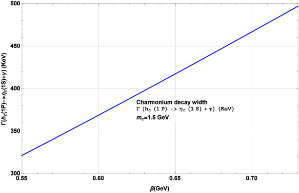
Figure 2: Decay width for $h_{c}(1P)\to\eta_{c}(1S)+\gamma$ (KeV) as a function of $\beta_{h_{c}(1P)(\eta_{c})(1S)}$ in LFQM, with $m_{c}=1.5$ GeV.

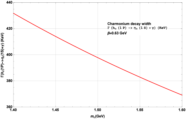
Figure 3: Decay width for $h_{c}(1P)\to\eta_{c}(1S)+\gamma$ (KeV) as a function of $m_{c}$ in the LFQM, with $\beta_{h_{c}(1P)(\eta_{c}(1S))}=0.63$ GeV.

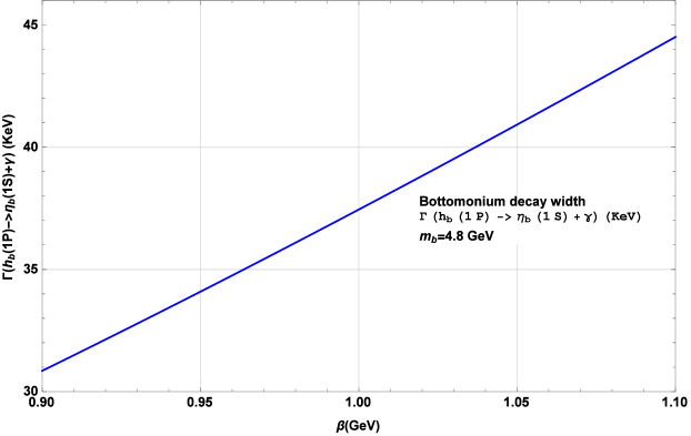
Figure 4: Decay width for $h_{b}(1P)\to\eta_{b}(1S)+\gamma$ (KeV) as a function of $\beta_{h_{b}(1P)(\eta_{b}(1S))}$ in the LFQM, with $m_{b}=4.8$ GeV.

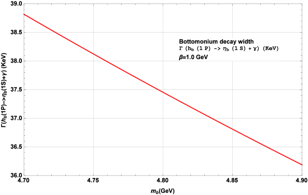
Figure 5: Decay width for $h_{b}(1P)\to\eta_{b}(1S)+\gamma$ (KeV) as a function of $m_{b}$ in the LFQM, with $\beta_{h_{b}(1P)(\eta_{b}(1S))}=1.0$ GeV.

In this section we apply the radiative transition formulas for the decay $1^{+-}({}^{1}P_{1})\to 0^{-+}({}^{1}S_{0})+\gamma$ in the framework of the light-front quark model, which we reviewed in Section II, to study the radiative decay of the $c\bar{c}$ state $h_{c1}(1P)$ via the channel $h_{c}(1P)\to\eta_{c}(1S)+\gamma$ and the $b\bar{b}$ state $h_{b}(1P)$ via the channel $h_{b}(1P)\to\eta_{b}(1S)+\gamma$. We present the results of our numerical calculations of decay widths. Our results extend those which we previously presented with Ke and Li in Ke:2013zs . For the charmonium $h_{c}(1P)$ radiative decay, we compare our result with experimental data on the width, as listed in the Particle Data Group Review of Particle Properties (RPP) PDG . We also list the theoretical calculations from other models, including non-relativistic potential model (NR)Brambilla:2004wf ; Barnes:2005pb ; Voloshin:2007dx , relativistic quark model (R)Ebert:2002pp , the Godfrey-Isgur potential model (GI)Barnes:2005pb , screened potential models with zeroth-order wavefunctions (${\text{SNR}}_{0}$) and first-order relativistically corrected wavefunctions (${\text{SNR}}_{1}$) Li:2009zu .

Although the PDG lists the width for the decay $h_{c}(1P)\to\eta_{c}(1S)+\gamma$, it does not list the width for the $h_{b}(1P)\to\eta_{b}(1S)+\gamma$ decay, only the branching ratio. Since our calculation yields the width itself, and a calculation of the branching ratio requires division by the total width, we therefore compare our results on the widths for these decays with predictions from other models, including the non-relativistic potential model (NR)Brambilla:2004wf , the relativistic quark model (R)Ebert:2002pp , the Godfrey-Isgur potential model (GI)Godfrey:2015dia , screened potential models with zeroth-order wave functions (${\text{SNR}}_{0}$) and first-order relativistically corrected wave functions(${\text{SNR}}_{1}$) Li:2009nr , as well as the nonrelativistic constituent quark model (CQM)Segovia:2016xqb .

First, we study the radiative decay $h_{c}(1P)\to\eta_{c}(1S)+\gamma$ in the LFQM, which depends on the corresponding harmonic oscillator wavefunction ($\beta_{h_{c}(\eta_{c})}$) and the effective charm quark mass, $m_{c}$. For the central values of $m_{c}$ and the wavefunction parameters $\beta$, we use the central values of these parameters suggested by previous study of LFQM Shi:2016nxr :

$$m_{c}=1.5\pm 0.1\ \text{GeV}\ .$$ (74)

$$\beta_{h_{c}(\eta_{c})}=0.63\pm 0.1\ \text{GeV}\ .$$ (75)

While Ref. Ke:2013zs allowed a 10 % variation in input parameters, we investigate a somewhat larger variation, as indicated in Eqs. (74) and (75). We present our numerical results in Table 1, with the uncertainties arising from the uncertainties in the $\beta$ parameters and the value of $m_{c}$. We also plot the predicted width as a function of the input values for the charm quark mass $m_{c}$ and wavefunction structure parameter $\beta_{h_{c}(\eta_{c})}$ in Fig. 2 and Fig. 3. From these results, we find that the main theoretical uncertainties come from variation of $\beta_{h_{c}(\eta_{c})}$. With the same central value for $\beta_{h_{c}(\eta_{c})}$ as was used in Ke:2013zs , we obtain a somewhat smaller central value for the width, namely 398 keV as contrasted with 685 keV in Ke:2013zs . As is evident from our Table 1, our current result for this width agrees well with experimental data within the range of experimental and theoretical uncertainties. The experimental data have substantial uncertainties, and our result is relatively close to the central experimental value, compared to other non-relativistic models.

Next we study radiative decay of $h_{b}(1P)\to\eta_{b}(1S)+\gamma$ in LFQM. For the central value of the effective bottom/beauty quark mass $m_{b}$, we use the value suggested by the previous LFQM study Ke:2013zs (see also Shi:2016nxr ). For the wavefunction parameter $\beta_{h_{b}(1P)(\eta_{b}(1S))}$, we estimate this to be in the range $\beta\sim 0.9-1.3\ \text{GeV}$, which is suggested in Godfrey:2015dia , where $\beta$ is fitted by equating the rms radius of the harmonic oscillator wavefunction for the specified states with the rms radius of the wavefunctions calculated using the relativized quark model. Our values for these input parameters are:

$$m_{b}=4.8\pm 0.1\ \text{GeV}\ .$$ (76)

$$\beta_{h_{b}(1P)(\eta_{b}(1S))}=1.0\pm 0.1\ \text{GeV}\ .$$ (77)

We list the numerical results in the LFQM in Table 2. For comparison, we also list other theoretical calculations from various types of models, including the non-relativistic potential model (NR)Brambilla:2004wf , the relativistic quark model (R)Ebert:2002pp , the Godfrey-Isgur potential model (GI)Godfrey:2015dia , screened potential models with zeroth-order wavefunctions (${\text{SNR}}_{0}$) and first-order relativistically corrected wavefunctions(${\text{SNR}}_{1}$) Li:2009nr and the non-relativistic constituent quark model (CQM)Segovia:2016xqb . As can be seen from Table 2, with the given range of uncertainties, our value agrees with predictions from the non-relativistic potential model (NR)Brambilla:2004wf , the Godfrey-Isgur potential model (GI)Godfrey:2015dia and screened potential models with relativistically corrected wavefunctions (${\text{SNR}}_{1}$) Li:2009nr . To show the theoretical uncertainties arising from uncertainties in the $\beta_{h_{b}(1P)(\eta_{b}(1S))}$ parameter and the value of $m_{b}$, we also plot the decay width for $h_{b}(1P)\to\eta_{b}(1S)+\gamma$ as a function of these parameters in Fig. 4 and Fig. 5. We find that the width is not very sensitive to the variation of $m_{b}$ and the main uncertainties arise from the uncertainty in the wavefunction parameter $\beta_{h_{b}(1P)(\eta_{b}(1S))}$.

These results show that the light-front quark model with phenomenological meson wavefunctions (specifically, harmonic oscillator wavefunctions) is suitable for the calculation of quarkonium ${}^{1}P_{1}\to{}^{1}S_{0}+\gamma$ radiative decay widths, since this model gives reasonable predictions for these widths, as compared with experimental data and other theoretical models.

V Conclusion

In this paper we have revisited the calculation of the radiative decay width of a $1^{+-}$ axial vector meson A to a $0^{-+}$ pseudoscalar meson P via the channel $1^{+-}\to 0^{-+}+\gamma$ in the LFQM approach, extending our previous work in Ref. Ke:2013zs . As part of our analysis, we have presented the reduction of the LFQM results in the non-relativistic limit and have shown the connection with the non-relativistic electric dipole transition formula for heavy quarkonium systems. We have then applied the LFQM formula to the radiative decays $h_{c}(1P)\to\eta_{c}(1S)+\gamma$ and $h_{b}(1P)\to\eta_{b}(1S)+\gamma$. We have performed numerical calculations and have compared our results with experimental data and other model predictions. We have shown that our results are in reasonable agreement with data and other model calculations.

Appendix A The wavefunctions

The normalization of the S-wave meson wavefunction in the light-front framework is

$$\frac{1}{2(2\pi)^{3}}\int dx_{2}dp^{2}_{\perp}\,|\varphi(x_{2},p_{\perp})|^{2}=1.$$ (78)

Here $\varphi(x_{2},p_{\perp})$ is related to the wavefunction in normal coordinates $\psi(p)$ by

$$\varphi(x_{2},p_{\perp})=4\pi^{\frac{3}{2}}\sqrt{\frac{dp_{z}}{dx_{2}}}\psi(p)\ ,\quad\frac{dp_{z}}{dx_{2}}=\frac{e^{\prime}_{1}e_{2}}{x_{1}x_{2}M^{\prime}_{0}}\$$ (79)

The normalization of $\psi(p)$ is given by

$$\int d{\bf p}^{3}\,|\psi(p)|^{2}=4\pi\int p^{2}dp\,|\psi(p)|^{2}=1\ .$$ (80)

The normalization for the P-wave meson wavefunction in the light-front framework is Cheng:2003sm

$$\frac{1}{2(2\pi)^{3}}\int dx_{2}dp^{2}_{\perp}\,|\varphi_{p}(x_{2},p_{\perp})|^{2}p_{i}p_{j}=\delta_{ij}\ ,$$ (81)

where $p_{i}=(p_{x},p_{y},p_{z})$. In terms of the P-wave wavefunction in normal coordinates,

$$\varphi_{p}(x_{2},p_{\perp})=4\pi^{\frac{3}{2}}\sqrt{\frac{dp_{z}}{dx_{2}}}\psi_{p}(p)\ ,\quad\frac{dp_{z}}{dx_{2}}=\frac{e^{\prime}_{1}e_{2}}{x_{1}x_{2}M^{\prime}_{0}}\ .$$ (82)

we have the following normalization condition:

$$\frac{1}{3}\cdot 4\pi\int^{\infty}_{0}|\psi_{p}(p)|^{2}p^{4}dp=1\ .$$ (83)

For the gaussian type 1P and 1S wavefunctions, we have the relation

$$\psi_{p}(p)=\sqrt{\frac{2}{\beta^{2}}}\psi(p)\ .$$ (84)

The explicit form of 1-S harmonic oscillator wavefunction in the light-front approach is given by Cheng:2003sm

$$\psi(p) = \left(\frac{1}{\beta^{2}\pi}\right)^{\frac{3}{4}}\exp\left(-\frac{1}{2}\frac{p^{2}}{\beta^{2}}\right)\ .$$ (85)

Appendix B Some expressions in the light-front formalism

In the covariant light-front formalism we have

$$M^{\prime 2}_{0} = (e^{\prime}_{1}+e_{2})^{2}=\frac{p^{\prime 2}_{\perp}+m^{\prime 2}_{1}}{x_{1}}+\frac{p^{\prime 2}_{\perp}+m^{2}_{2}}{x_{2}}$$

$$M^{\prime\prime 2}_{0} = (e^{\prime\prime}_{1}+e_{2})^{2}=\frac{p^{\prime\prime 2}_{\perp}+m^{\prime\prime 2}_{1}}{x_{1}}+\frac{p^{\prime\prime 2}_{\perp}+m^{2}_{2}}{x_{2}}$$

$$\tilde{M}^{\prime}_{0} = \sqrt{M^{\prime 2}_{0}-(m^{\prime}_{1}-m_{2})^{2}}$$

$$\tilde{M}^{\prime\prime}_{0} = \sqrt{M^{\prime\prime 2}_{0}-(m^{\prime\prime}_{1}-m_{2})^{2}}$$

$$p^{\prime}_{z} = \frac{x_{2}M^{\prime}_{0}}{2}-\frac{m^{2}_{2}+p^{\prime 2}_{\perp}}{2x_{2}M^{\prime}_{0}}$$

$$p^{\prime\prime}_{z} = \frac{x_{2}M^{\prime\prime}_{0}}{2}-\frac{m^{2}_{2}+p^{\prime\prime 2}_{\perp}}{2x_{2}M^{\prime\prime}_{0}}.$$ (86)

The explicit expressions for $A^{(i)}_{j}(i,j=1\sim 4)$ and $Z_{2}$ are

$$A^{(1)}_{1}=\frac{x_{1}}{2}\ ,\ A^{(1)}_{2}=A^{(1)}_{1}-\frac{p^{\prime}_{\perp}\cdot q_{\perp}}{q^{2}}\ ,$$

$$A^{(2)}_{1}=-p^{\prime 2}_{\perp}-\frac{(p^{\prime}_{\perp}\cdot q_{\perp})^{2}}{q^{2}},\ A^{(2)}_{2}=(A^{(1)}_{1})^{2},$$

$$A^{(2)}_{3}=A^{(1)}_{1}A^{(1)}_{2}\ ,\ A^{(2)}_{4}=(A^{(1)}_{2})^{2}-\frac{1}{q^{2}}A^{(2)}_{1}\ ,$$

$$A^{(3)}_{1}=A^{(1)}_{1}A^{(2)}_{1}\ ,A^{(3)}_{2}=A^{(1)}_{2}A^{(2)}_{1}\ ,$$

$$A^{(3)}_{3}=A^{(1)}_{1}A^{(2)}_{2}\ ,A^{(3)}_{4}=A^{(1)}_{2}A^{(2)}_{2}\ .$$ (87)

$$Z_{2}=\hat{N}^{\prime}_{1}+m^{\prime 2}_{1}-m^{2}_{2}+(1-2x_{1})M^{\prime 2}+(q^{2}+q\cdot P)\frac{p^{\prime}_{\perp}\cdot q_{\perp}}{q^{2}}.$$ (88)

References

- (1) J. J. Aubert et al., Phys. Rev. Lett. 33, 1404 (1974).
- (2) J. E. Augustin et al., Phys. Rev. Lett. 33, 1406 (1974).
- (3) S. W. Herb et al., Phys. Rev. Lett. 39, 252 (1977).
- (4) W. R. Innes et al., Phys. Rev. Lett. 39, 1240 (1977).
- (5) C. Quigg and J. L. Rosner, Phys. Rept. 56, 167 (1979).
- (6) H. Grosse and A. Martin, Phys. Rept. 60, 341 (1980).
- (7) P. Franzini and J. Lee-Franzini, Phys. Rept. 81, 239 (1982).
- (8) W. Kwong, J. L. Rosner, C. Quigg, Ann. Rev. Nucl. Part. Sci. 37, 325 (1987).
- (9) N. Brambilla et al. [Quarkonium Working Group Collaboration], hep-ph/0412158.
- (10) E. Eichten, S. Godfrey, H. Mahlke, and J. L. Rosner, Rev. Mod. Phys. 80, 1161 (2008).
- (11) M. B. Voloshin, Prog. Part. Nucl. Phys. 61, 455 (2008)
- (12) K. Berkelman and E. H. Thorndike, Ann. Rev. Nucl. Part. Sci. 59, 297 (2009).
- (13) N. Brambilla et al., Eur. Phys. J. C 71, 1534 (2011).
- (14) J. L. Rosner, in Proc. of Ninth International Conference on Flavor Physics and CP Violation (FPCP 2011, Israel), arXiv:1107.1273.
- (15) C. Patrignani, T. K., and J. Rosner, Annu. Rev. Nucl. Part. Sci. 63, 21 (2013).
- (16) G. Karl, S. Meshkov and J. L. Rosner, Phys. Rev. Lett. 45, 215 (1980).
- (17) P. Moxhay and J. L. Rosner, Phys. Rev. D 28, 1132 (1983).
- (18) R. McClary and N. Byers, Phys. Rev. D 28, 1692 (1983).
- (19) H. Grotch, D. A. Owen and K. J. Sebastian, Phys. Rev. D 30, 1924 (1984).
- (20) D. Ebert, R. N. Faustov and V. O. Galkin, Phys. Rev. D 67, 014027 (2003).
- (21) B. Q. Li and K. T. Chao, Commun. Theor. Phys. 52, 653 (2009).
- (22) S. Godfrey and K. Moats, Phys. Rev. D 92, 054034 (2015).
- (23) J. Segovia, P. G. Ortega, D. R. Entem and F. Fernandez, Phys. Rev. D 93, 074027 (2016).
- (24) N. Brambilla, Y. Jia and A. Vairo, Phys. Rev. D 73, 054005 (2006)
- (25) T. Barnes, S. Godfrey and E. S. Swanson, Phys. Rev. D 72, 054026 (2005)
- (26) B. Q. Li and K. T. Chao, Phys. Rev. D 79, 094004 (2009)
- (27) C. Patrignani et al. (Particle Data Group), Chin. Phys. C, 40, 100001 (2016); online at http://pdg.lbl.gov.
- (28) M. V. Terentev, Sov. J. Nucl. Phys. 24, 106 (1976) [Yad. Fiz. 24, 207 (1976)].
- (29) V. B. Berestetsky and M. V. Terentev, Sov. J. Nucl. Phys. 24, 547 (1976) [Yad. Fiz. 24, 1044 (1976)].
- (30) G. P. Lepage and S. J. Brodsky, Phys. Rev. D 22, 2157 (1980).
- (31) P. L. Chung, F. Coester and W. N. Polyzou, Phys. Lett. B 205, 545 (1988).
- (32) S. J. Brodsky, H. C. Pauli and S. S. Pinsky, Phys. Rept. 301, 299 (1998)
- (33) S. J. Brodsky and G. F. de Teramond, Phys. Rev. Lett. 96, 201601 (2006); G. F. de Teramond and S. J. Brodsky, Phys. Rev. Lett. 102, 081601 (2009); S. J. Brodsky and G. F. de Teramond, Acta Phys. Polon. B 41, 2605 (2010).
- (34) S. J. Brodsky, G. F. de Teramond. H. G. Dosch, and J. Erlich, Phys. Rept. 584, 1 (2015).
- (35) W. Jaus, Phys. Rev. D 41, 3394 (1990); W. Jaus, Phys. Rev. D 44, 2851 (1991).
- (36) W. Jaus, Phys. Rev. D 60, 054026 (1999).
- (37) H. Y. Cheng, C. Y. Cheung and C. W. Hwang, Phys. Rev. D 55, 1559 (1997).
- (38) H. Y. Cheng, C. K. Chua and C. W. Hwang, Phys. Rev. D 69, 074025 (2004).
- (39) C. W. Hwang and Z. T. Wei, J. Phys. G 34, 687 (2007)
- (40) H. M. Choi, Phys. Rev. D 75, 073016 (2007).
- (41) C. W. Hwang and R. S. Guo, Phys. Rev. D 82, 034021 (2010)
- (42) H. W. Ke, X. Q. Li, Z. T. Wei and X. Liu, Phys. Rev. D 82, 034023 (2010).
- (43) H.-W. Ke, X.-Q. Li and Y.-L. Shi, Phys. Rev. D 87, 054022 (2013).
- (44) Y.-L. Shi, arXiv:1611.03712 [hep-ph].
- (45) F. Daghighian and D. Silverman, Phys. Rev. D 36, 3401 (1987).
- (46) D. Faiman and A. W. Hendry, Phys. Rev. 173, 1720 (1968).