Study of lattice QCD at finite chemical potential using canonical ensemble approach

Abstract

New approach to computation of canonical partition functions in $N_{f}=2$ lattice QCD is presented. We compare results obtained by new method with results obtained by known method of hopping parameter expansion. We observe agreement between two methods indicating validity of the new method. We use results for the number density obtained in the confining and deconfining phases at imaginary chemical potential to determine the phase transition line at real chemical potential.

1 Introduction

Recent results of heavy ion collision experiments at RHIC Adams:2005dq and LHC Aamodt:2008zz shed some light on properties of the quark gluon plasma and the position of the transition line in the temperature â baryon density plane. New experiments will be carried out at FAIR (GSI) and NICA (JINR). To fully explore the phase diagram theoretically it is necessary to make computations at finite temperature and finite baryon chemical potential. For finite temperature lattice QCD is the only ab-initio method available and many results had been obtained. However, for finite baryon density lattice QCD faces the so-called complex action problem (or sign problem). Various proposals exist at the moment to solve this problem see, e.g. reviews Muroya:2003qs ; Philipsen:2005mj ; deForcrand:2010ys and yet it is still very hard to get reliable results at $\mu_{B}/T>1$. Our work is devoted to developing the canonical partition function approach.

The fermion determinant at nonzero baryon chemical potential $\mu_{B}$, $\det\Delta(\mu_{B})$, is in general not real. This makes impossible to apply standard Monte Carlo techniques to computations with the partition function

$$Z_{GC}(\mu_{q},T,V)=\int\mathcal{D}U(\det\Delta(\mu_{q}))^{N_{f}}e^{-S_{G}},$$ (1)

where $S_{G}$ is a gauge field action, $\mu_{q}=\mu_{B}/3$ is quark chemical potential, $T=1/(aN_{t})$ is temperature, $V=(aN_{s})^{3}$ is volume, $a$ is lattice spacing, $N_{t},N_{s}$ - number of lattice sites in time and space directions.

The canonical approach was studied in a number of papers deForcrand:2006ec ; Ejiri:2008xt ; Li:2010qf ; Li:2011ee ; Danzer:2012vw ; Gattringer:2014hra ; Fukuda:2015mva ; Nakamura:2015jra . It is based on the following relations. Relation between grand canonical partition function $Z_{GC}(\mu_{q},T,V)$ and the canonical one $Z_{C}(n,T,V)$ called fugacity expansion:

$$Z_{GC}(\mu,T,V)=\sum_{n=-\infty}^{\infty}Z_{C}(n,T,V)\xi^{n},$$ (2)

where $\xi=e^{\mu_{q}/T}$ is the fugacity. The inverse of this equation can be presented in the following form Hasenfratz:1991ax

$$Z_{C}\left(n,T,V\right)=\int_{0}^{2\pi}\frac{d\theta}{2\pi}e^{-in\theta}Z_{GC}(\theta,T,V).$$ (3)

$Z_{GC}(\theta,T,V)$ is the grand canonical partition function for imaginary chemical potential $\mu_{q}=i\mu_{qI}\equiv iT\theta$. Standard Monte Carlo simulations are possible for this partition function since fermionic determinant is real for imaginary $\mu_{q}$.

The QCD partition function $Z_{GC}$ is a periodic function of $\theta$: $Z_{GC}(\theta)=Z_{GC}(\theta+2\pi/3)$. This symmetry is called Roberge-Weiss symmetry Roberge:1986mm . As a consequence of this periodicity the canonical partition functions $Z_{C}(n,T,V)$ are nonzero only for $n=3k$. QCD possesses a rich phase structure at nonzero $\theta$, which depends on the number of flavors $N_{f}$ and the quark mass $m$. This phase structure is shown in Fig. 1. $T_{c}$ is the confinement/deconfinement crossover point at zero chemical potential. The line $(T\geq T_{RW},\mu_{I}/T=\pi/3)$ indicates the first order phase transition. On the curve between $T_{c}$ and $T_{RW}$, the transition is expected to change from the crossover to the first order for small and large quark masses, see e.g. Bonati:2014kpa .

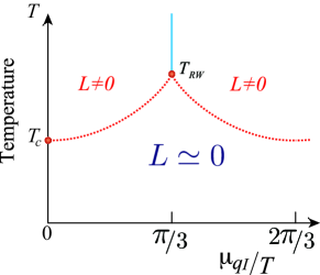
Figure 1: Schematical figure of Roberge-Weiss phase structure in the pure imaginary chemical potential regions.

Quark number density $n_{q}$ for $N_{f}$ degenerate quark flavours is defined by the following equation:

$$\frac{n_{q}}{T^{3}}=\frac{1}{VT^{2}}\frac{\partial}{\partial\mu_{q}}\ln Z_{GC}=\frac{N_{f}N_{t}^{3}}{N_{s}^{3}Z_{GC}}\int\mathcal{D}Ue^{-S_{G}}(\det\Delta(\mu_{q}))^{N_{f}}\mathrm{tr}\left[\Delta^{-1}\frac{\partial\Delta}{\partial\mu_{q}/T}\right].$$ (4)

It can be computed numerically for imaginary chemical potential. Note, that for the imaginary chemical potential $n_{q}$ is also purely imaginary: $n_{q}=in_{qI}$.

From eqs. (2) and (4) it follows that densities $n_{q}$ and $n_{qI}$ are related to $Z_{C}(n,T,V)$ (below we will use the notation $Z_{n}$ for the ratio $Z_{C}(n,T,V)/Z_{C}(0,T,V)$) by equations

$$n_{q}/T^{3}={\cal{N}}\frac{2\sum_{n>0}nZ_{n}\sinh(n\theta)}{1+2\sum_{n>0}Z_{n}\cosh(n\theta)},\,\,n_{qI}/T^{3}={\cal{N}}\frac{2\sum_{n>0}nZ_{n}\sin(n\theta)}{1+2\sum_{n>0}Z_{n}\cos(n\theta)}\,,$$ (5)

where ${\cal{N}}$ is a normalization constant, ${\cal{N}}=\frac{N_{t}^{3}}{N_{s}^{3}}$. Our suggestion is to compute $Z_{n}$ using equation (5) for $n_{qI}$.

One can compute $Z_{GC}(\theta,T,V)$ using numerical data for $n_{qI}/T^{3}$ via numerical integration

$$L_{Z}(\theta)\equiv\log\frac{Z_{GC}(\theta,T,V)}{Z_{GC}(0,T,V)}=-V\int_{0}^{\theta}d\tilde{\theta}\leavevmode\nobreak\ n_{qI}(\tilde{\theta})\,,$$ (6)

where we omitted $T$ and $V$ from the grand canonical partition function notation. Then $Z_{n}$ can be computed as

$$Z_{n}=\frac{\int_{0}^{2\pi}\frac{d\theta}{2\pi}e^{-in\theta}e^{L_{Z}(\theta)}}{\int_{0}^{2\pi}\frac{d\theta}{2\pi}e^{L_{Z}(\theta)}}$$ (7)

In our work we use modified version of this approach Bornyakov:2016 . Instead of numerical integration in (6) we fitted $n_{qI}/T^{3}$ to theoretically motivated functions of $\mu_{qI}$. It is known that the density of noninteracting quark gas is described by

$$n_{q}/T^{3}=N_{f}\Bigl{(}2\frac{\mu_{q}}{T}+\frac{2}{\pi^{2}}\Bigl{(}\frac{\mu_{q}}{T}\Bigr{)}^{3}\Bigr{)}.$$ (8)

We thus fit the data for $n_{qI}$ to an odd power polynomial of $\theta$

$$n_{qI}(\theta)/T^{3}=\sum_{n=1}^{n_{max}}a_{2n-1}\theta^{2n-1}\,,$$ (9)

in the deconfining phase. This type of the fit was also used in Ref. Takahashi:2014rta and Ref. Gunther:2016vcp .

In the confining phase (below $T_{c}$) the hadron resonance gas model provides good description of the chemical potential dependence of thermodynamic observables Karsch:2003zq . Thus it is reasonable to fit the density to a Fourier expansion

$$n_{qI}(\theta)/T^{3}=\sum_{n=1}^{n_{max}}f_{3n}\sin(3n\theta)$$ (10)

Again this type of the fit was used in Ref. Takahashi:2014rta and conclusion was made that it works well.

To demonstrate our method we made simulations of the lattice QCD with $N_{f}=2$ clover improved Wilson quarks and Iwasaki improved gauge field action, for detailed definition of the lattice action see Bornyakov:2016 . We simulate $16^{3}\times 4$ lattices at temperatures $T/T_{c}=1.35,1.20$ and 1.08 in the deconfinemnt phase and $0.99,0.93,0.84$ in the confinement phase along the line of constant physics with $m_{\pi}/m_{\rho}=0.8$. All parameters of the action, including $c_{SW}$ value were borrowed from the WHOT-QCD collaboration paper Ejiri:2009hq . We compute the number density on samples of $N_{conf}$ configurations with $N_{conf}=1800$, using every 10-th trajectory produced with Hybrid Monte Carlo algorithm.

2 Results

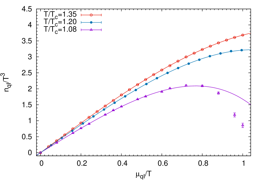
Figure 2: Imaginary density as function of $\theta$ in the deconfinement phase at temperatures $T/T_{c}=1.35,1.20,1.08$. The curves show fits to function (9).

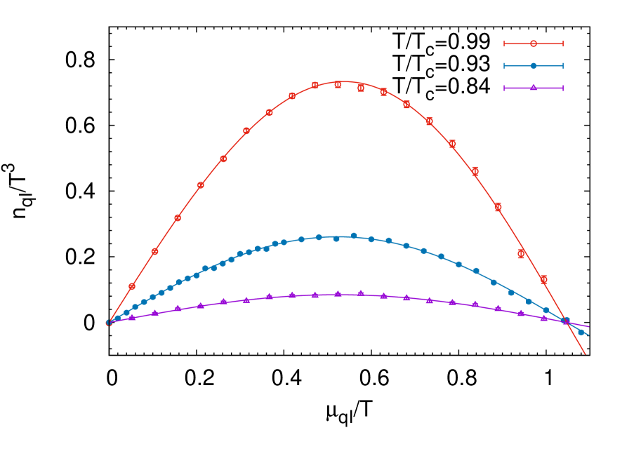
Figure 3: Imaginary density as function of $\theta$ for temperatures in the confining phase. The curves show fits to (10) with $n_{max}=1$ for $T/T_{c}=0.84,0.93$ and $n_{max}=2$ for $T/T_{c}=0.99$.

In Fig. 3 and Fig. 3 we show numerical results for $n_{qI}$ as a function of $\theta$ in deconfining and confining phases, respectively Bornyakov:2016 .

Note, that behavior of $n_{qI}$ at $T=1.08$ is different from that at higher temperatures. This temperature is below $T_{RW}$ and at $\theta=\pi/3$ there is no first order phase transition, $n_{qI}$ is continuous. Instead there is a crossover to the confinement phase at about $\theta=0.92(2)$.

It is not yet clear how to fit the data over the range of $\mu_{qI}$ covering both deconfining and confining phase. Here we use fit to function (9) with $n_{max}=3$ over the range $[0,0.8]$, i.e. including only the deconfining phase. In this case we should consider the fit as a Taylor expansion.

We computed $Z_{n}$ using new procedure described in the previous section and compared with results obtained with use of the hopping parameter expansion. We found good agreement between two methods indicating that the new method works well Bornyakov:2016 . This allows us to make analytical continuation to the real values of $\mu_{q}$ beyond the Taylor expansion validity range (for all temperatures apart from $T/T_{c}=1.08$). Respective results are shown in Fig. 5.

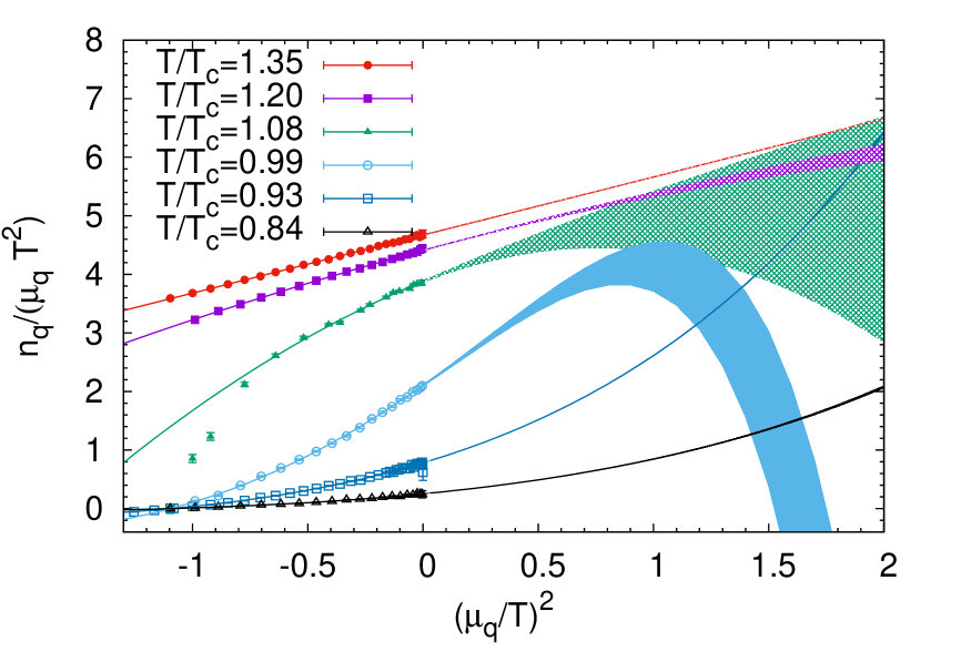
Figure 4: Analytical continuation for the number density vs. $\mu_{q}^{2}$. The curves show respective fits eq. (9) or eq. (10). The width of the curves indicates the statistical error of extrapolation to $\mu_{q}^{2}>0$.

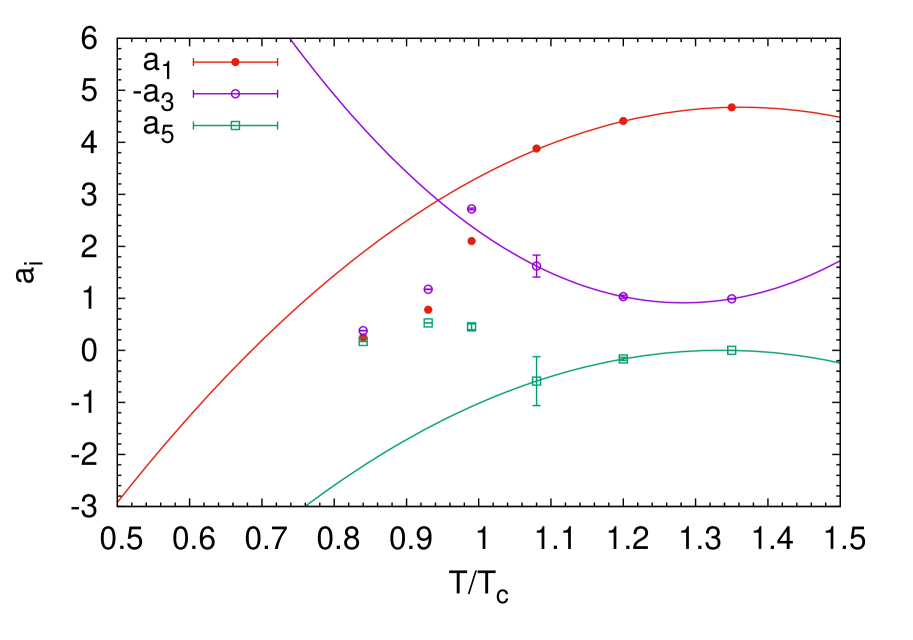
Figure 5: Constants $a_{i}$ of eq. (9) for six values of temperature. The curves show polynomial fits over $T>T_{c}$ range.

Using the results for the number density $n_{q}$ we can compute the temperature of the transition from the hadron phase to quark-gluon plasma phase using the following procedure. Our results for the number density at temperatures $T>T_{c}$ as function of the chemical potential $\mu_{q}$ are reliable even for large $\mu_{q}$ for $T>T_{RW}$, while for $T_{c}<T<T_{RW}$ they are reliable at the moment for small $\mu_{q}$ only. We can use these results to compute the pressure $\Delta P_{deconf}(T,\mu_{q})=P(T,\mu_{q})-P(T,0)$ as function of $\mu_{q}$ and then extrapolate pressure for fixed $\mu_{q}$ to temperatures $T<T_{c}$. To get good extrapolation we need pressure computed for more values of temperature than is available now but three values which we have in this work is enough to demonstrate the idea. We then find the transition temperature $T_{c}(\mu_{q})$ solving numerically equation $\Delta P_{deconf}(T,\mu_{q})=\Delta P_{conf}(T,\mu_{q})$, where $\Delta P_{conf}(T,\mu_{q})$ is pressure computed from results for the number density $n_{q}$ we obtained in the confinement phase. In this paper we use extrapolation for the coefficients in (9) rather than for pressure itself. This extrapolation is shown in Fig. 5. We fitted the data for $a_{i},i=1,3,5$ by a polynomial $b_{0}+b_{1}\frac{T}{T_{c}}+b_{2}\left(\frac{T}{T_{c}}\right)^{2}$ and then computed the extrapolated values of these parameters at $T/T_{c}=0.93$ and 0.84. The extrapolated values were used to compute $\Delta P_{deconf}(T,\mu_{q})/T^{4}$ as

$$\frac{\Delta P_{deconf}(T,\mu_{q})}{T^{4}}=\frac{a_{1}}{2}\left(\frac{T}{T_{c}}\right)^{2}-\frac{a_{3}}{4}\left(\frac{T}{T_{c}}\right)^{4}+\frac{a_{5}}{6}\left(\frac{T}{T_{c}}\right)^{6}$$ (11)

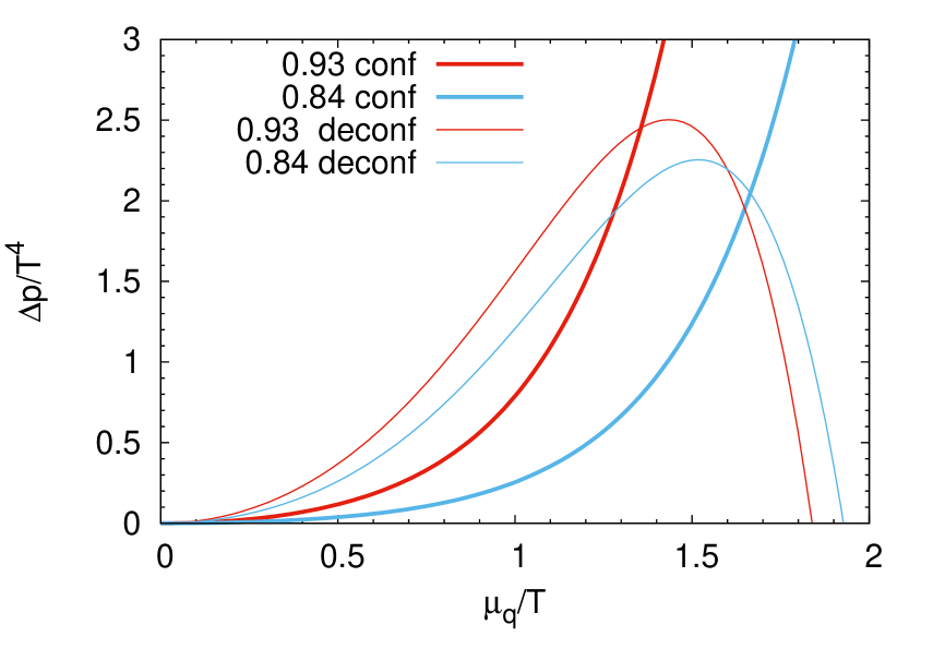
Figure 6: Pressure computed via eq. (11) (denoted by ’deconf’, thin curves) and by integration of eq. (10) (denoted by ’conf’, thick curves) for $T/T_{c}=0.93,0.84$.

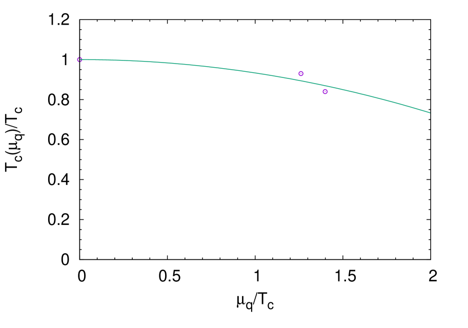
Figure 7: Transition line in the temperature - chemical potential plane. The curve show quadratic fit.

We show results in Fig. 7 together with pressure computed by integration of eq. (10) for $T/T_{c}=0.93,0.84$. The crossing points determine values of $\mu_{q}$ on transition line at respective value of temperature. We show the coordinates of these crossing points in Fig. 7 together with fit of the form

$$T_{c}(\mu_{q})/T_{c}=1-C\left(\mu_{q}/T_{c}\right)^{2}$$ (12)

The result for the fit parameter is $C=0.07$. We have to emphasize that in Figs. 7 and  7 we do not show statistical or systematic errors since we are not yet able to compute them. These figures are shown to illustrate our idea about the method to compute the transition temperature dependence on the chemical potential. Still it is encouraging that the value of the coefficient $C$ obtained is of correct order of magnitude. We can compare with Refs. deForcrand:2002hgr ; Wu:2006su where $C=0.051(3)$ and $C=0.065(7)$ respectively were found in lattice QCD with $N_{f}=2$. In both papers analytical continuation of $\frac{T_{c}(\mu_{q})}{T_{c}}$ from imaginary $\mu_{q}$ was used.

Thus we presented new method to compute the canonical partition functions $Z_{n}$. It is based on fitting of the imaginary number density for all values of imaginary chemical potential to the theoretically motivated fitting functions: polynomial fit (9) in the deconfinement phase for $T$ above $T_{RW}$ and Fourier-type fit (10) in the confinement phase. We also explained how the transition line at real $\mu_{q}$ can be computed using results we obtained for the number density $n_{q}$. We are planning to increase the number of temperature values to improve the precision of this method. It is worth to note that the method of direct analytical continuation for $\frac{T_{c}(\mu_{q})}{T_{c}}$ from imaginary chemical potential can be applied to our data. This will help us to improve the method presented here.

Acknowledgments
This work was completed due to support by RSF grant under contract 15-12-20008. Computer simulations were performed on the FEFU GPU cluster Vostok-1 and MSU ’Lomonosov’ supercomputer.

References

- (1) J. Adams et al. (STAR), Nucl. Phys. A757, 102 (2005), nucl-ex/0501009
- (2) K. Aamodt et al. (ALICE), JINST 3, S08002 (2008)
- (3) S. Muroya, A. Nakamura, C. Nonaka, T. Takaishi, Prog. Theor. Phys. 110, 615 (2003), hep-lat/0306031
- (4) O. Philipsen, PoS LAT2005, 016 (2006), [PoSJHW2005,012(2006)], hep-lat/0510077
- (5) P. de Forcrand, PoS LAT2009, 010 (2009), 1005.0539
- (6) P. de Forcrand, S. Kratochvila, Nucl. Phys. Proc. Suppl. 153, 62 (2006), [,62(2006)], hep-lat/0602024
- (7) S. Ejiri, Phys. Rev. D78, 074507 (2008), 0804.3227
- (8) A. Li, A. Alexandru, K.F. Liu, X. Meng, Phys. Rev. D82, 054502 (2010), 1005.4158
- (9) A. Li, A. Alexandru, K.F. Liu, Phys. Rev. D84, 071503 (2011), 1103.3045
- (10) J. Danzer, C. Gattringer, Phys. Rev. D86, 014502 (2012), 1204.1020
- (11) C. Gattringer, H.P. Schadler, Phys. Rev. D91, 074511 (2015), 1411.5133
- (12) R. Fukuda, A. Nakamura, S. Oka, Phys. Rev. D93, 094508 (2016), 1504.06351
- (13) A. Nakamura, S. Oka, Y. Taniguchi, JHEP 02, 054 (2016), 1504.04471
- (14) A. Hasenfratz, D. Toussaint, Nucl. Phys. B371, 539 (1992)
- (15) A. Roberge, N. Weiss, Nucl. Phys. B275, 734 (1986)
- (16) C. Bonati, P. de Forcrand, M. D’Elia, O. Philipsen, F. Sanfilippo, Phys. Rev. D90, 074030 (2014), 1408.5086
- (17) V.G. Bornyakov, D.L. Boyda, V.A. Goy, A.V. Molochkov, A. Nakamura, A.A. Nikolaev, V.I. Zakharov (2016), 1611.04229
- (18) J. Takahashi, H. Kouno, M. Yahiro, Phys. Rev. D91, 014501 (2015), 1410.7518
- (19) J. Gunther, R. Bellwied, S. Borsanyi, Z. Fodor, S.D. Katz, A. Pasztor, C. Ratti (2016), 1607.02493
- (20) F. Karsch, K. Redlich, A. Tawfik, Phys. Lett. B571, 67 (2003), hep-ph/0306208
- (21) S. Ejiri, Y. Maezawa, N. Ukita, S. Aoki, T. Hatsuda, N. Ishii, K. Kanaya, T. Umeda (WHOT-QCD), Phys. Rev. D82, 014508 (2010), 0909.2121
- (22) P. de Forcrand, O. Philipsen, Nucl. Phys. B642, 290 (2002), hep-lat/0205016
- (23) L.K. Wu, X.Q. Luo, H.S. Chen, Phys. Rev. D76, 034505 (2007), hep-lat/0611035