Multiscale and multilevel technique for consistent segmentation of nonstationary time series

Abstract

In this paper, we propose a fast, well-performing, and consistent method for segmenting a piecewise-stationary, linear time series with an unknown number of breakpoints. The time series model we use is the nonparametric Locally Stationary Wavelet model, in which a complete description of the piecewise-stationary second-order structure is provided by wavelet periodograms computed at multiple scales and locations. The initial stage of our method is a new binary segmentation procedure, with a theoretically justified and rapidly computable test criterion that detects breakpoints in wavelet periodograms separately at each scale. This is followed by within-scale and across-scales post-processing steps, leading to consistent estimation of the number and locations of breakpoints in the second-order structure of the original process. An extensive simulation study demonstrates good performance of our method.

keywords: binary segmentation, breakpoint detection, locally stationary wavelet model, piecewise stationarity, post-processing, wavelet periodogram.

1 Introduction

A stationarity assumption is appealing when analysing short time series. But, it is often unrealistic, for example when observing time series evolving in naturally nonstationary environments. One such example can be found in econometrics, where price processes are considered to have time-varying variance in response to events taking place in the market; Mikosch and Stărică (1999), Kokoszka and Leipus (2000), and Stărică and Granger (2005), among others, argued in favour of nonstationary modelling of financial returns. For example, given the explosion of market volatility during the recent financial crisis, it is unlikely that the same stationary time series model can accurately describe the evolution of market prices before and during the crisis.

Piecewise stationarity is a well studied and arguably the simplest form of departure from stationarity, and one task of interest is to detect breakpoints in the dependence structure. Breakpoint detection has received considerable attention and the methods that have been developed can be broadly categorized into retrospective (a posteriori) methods and on-line methods. In the interest of space, we do not review on-line breakpoint detection approaches here but refer the reader to Lai (2001).

The “a posteriori” approach takes into account the entire set of observations at once and detects breakpoints which occurred in the past. Our interest here lies in the “a posteriori” segmentation category, and we propose a retrospective segmentation procedure that achieves consistency in identifying multiple breakpoints for a class of nonstationary processes. (Note that we use the term “segmentation” interchangeably with “multiple breakpoint detection”.)

Early segmentation literature was mostly devoted to testing the existence of a single breakpoint in the mean or variance of independent observations (Chernoff and Zacks (1964), Sen and Srivastava (1975), Hawkins (1977), Hsu (1977), Worsley (1986)). When the presence of more than one breakpoint is suspected, an algorithm for detecting multiple breakpoints is needed. In Vostrikova (1981), a “binary segmentation” procedure was introduced, a computationally efficient multilevel breakpoint detection procedure that recursively locates and tests for multiple breakpoints, producing consistent breakpoint estimators for a class of random processes with piecewise constant means. However, the critical values of the tests at each stage are difficult to compute in practice due to stochasticity in previously selected breakpoints. Venkatraman (1993) employed the same procedure to find multiple breakpoints in the mean of independent and normally distributed variables and showed the consistency of the detected breakpoints with the tests depending on the sample size only, and thus are easier to compute. The binary segmentation procedure was also adopted to detect multiple shifts in the variance of independent observations (Inclán and Tiao (1994), Chen and Gupta (1997)).

Various multiple breakpoint detection methods have been proposed for time series of dependent observations. In Lavielle and Moulines (2000), least squares estimators of breakpoint locations were developed for linear processes with changing mean, extending the work of Bai and Perron (1998). Adak (1998) and Ombao et al. (2001) proposed methods that divided the time series into dyadic blocks and chose the best segmentation according to suitably tailored criteria. Whitcher et al. (2000, 2002) and Gabbanini et al. (2004) suggested segmenting long memory processes by applying the iterative cumulative sum of squares (ICSS) algorithm (proposed in Inclán and Tiao (1994)) to discrete wavelet coefficients of the process which were approximately Gaussian and decorrelated. Davis, Lee, and Rodriguez-Yam (2006) developed the Auto-PARM procedure which found the optimal segmentation of piecewise stationary AR processes via the minimum description length principle, later extended to the segmentation of non-linear processes in Davis et al. (2008). In Lavielle and Teyssière (2005), a breakpoint detection method was developed for weakly or strongly dependent processes with time-varying volatility that minimises a penalised contrast function based on a Gaussian likelihood. Andreou and Ghysels (2002) studied a heuristic segmentation procedure for the GARCH model with changing parameters, based on the work of Lavielle and Moulines (2000).

The aim of our work is to propose a well-performing, theoretically tractable, and fast procedure for detecting breakpoints in the second-order structure of a piecewise stationary time series that is linear but otherwise does not follow any particular parametric model. The nonparametric model we use for this purpose is the Locally Stationary Wavelet (LSW) model first proposed by Nason, von Sachs and Kroisandt (2000) and later studied by Fryzlewicz and Nason (2006) and Van Bellegem and von Sachs (2008). Detailed justification of our model choice is given in Section 2. In the LSW model, the piecewise constant second-order structure of the process is completely described by local wavelet periodograms at multiple scales, and it is those basic statistics that we use as a basis of our segmentation procedure.

To achieve the multiple breakpoint detection, we propose a binary segmentation method that is applied to wavelet periodograms separately at each scale, and followed by a within-scale and across-scales post-processing procedure to obtain consistent estimators of breakpoints in the second-order structure of the process. We note that wavelet periodograms follow a multiplicative statistical model, but our binary segmentation procedure is different from previously proposed binary segmentation methods for multiplicative models (Inclán and Tiao (1994), Chen and Gupta (1997)) in that it allows for correlated data, which is essential when working with wavelet periodograms. We note that Kouamo, Moulines, and Roueff (2010) proposed a CUSUM-type test for detecting a single change in the wavelet variance at one or several scales that also permits correlation in the data. We emphasise other unique ingredients of our breakpoint detection procedure which lead to its good performance and consistency in probability: the theoretical derivation of our test criterion (which only depends on the length of the time series and is thus fast to compute); the novel across-scales post-processing step, essential in combining the results of the binary segmentation procedures performed for each wavelet periodogram scale separately. We note that our method can simultaneously be termed “multiscale” and “multilevel”, as the basic time series model used for our purpose is wavelet-based and thus is a “multiscale” model, and the core methodology to segment each scale of the wavelet periodogram in the model is based on binary segmentation and is thus a “multilevel” procedure.

The paper is organised as follows. Section 2 explains the LSW model and justifies its choice. Our breakpoint detection methodology (together with the post-processing steps) is introduced in Section 3, where we also demonstrate its theoretical consistency in estimating the total number and locations of breakpoints. In Section 4, we describe the outcome of an extensive simulation study that demonstrates the good performance of our method. In Section 5, we apply our technique to the segmentation of the Dow Jones index and this results in the discovery of two breakpoints: one coinciding with the initial period of the recent financial crisis, and the other coinciding with the collapse of Lehman Brothers, a major financial services firm. The proofs of our theoretical results are provided in the Appendix. Software (an R script) implementing our methodology is available from: http://personal.lse.ac.uk/choh1/msml_technique.html.

2 Locally stationary wavelet time series

In this section, we define the Locally Stationary Wavelet (LSW) time series model (noting that our definition is a slight modification of that of Fryzlewicz and Nason (2006)), describe its properties, and justify its choice as an attractive framework for developing our time series segmentation methodology.

Definition 1.

A triangular stochastic array $\{X_{t,T}\}_{t=0}^{T-1}$ for $T=1,2,\ldots,$ is in a class of Locally Stationary Wavelet (LSW) processes if there exists a mean-square representation

$$X_{t,T}=\sum_{i=-\infty}^{-1}\sum_{k=-\infty}^{\infty}W_{i}(k/T)\psi_{i,t-k}\xi_{i,k}$$ (1)

with $i\in\{-1,-2,\ldots\}$ and $k\in\mathbb{Z}$ as scale and location parameters, respectively, the $\mathbf{\psi}_{i}=(\psi_{i,0},\ldots,\psi_{i,\mathcal{L}_{i}-1})$ are discrete, real-valued, compactly supported, non-decimated wavelet vectors with support lengths $\mathcal{L}_{i}=O(2^{-i})$, and the $\xi_{i,k}$ are zero-mean, orthonormal, identically distributed random variables. For each $i\leq-1$, $W_{i}(z):[0,1]\rightarrow\mathcal{R}$ is a real-valued, piecewise constant function with a finite (but unknown) number of jumps. If the $L_{i}$ denote the total magnitude of jumps in $W_{i}^{2}(z)$, the variability of functions $W_{i}(z)$ is controlled so that

• $\sum_{i=-\infty}^{-1}W_{i}^{2}(z)<\infty$ uniformly in $z$,

• $\sum_{i=-I}^{-1}2^{-i}L_{i}=O(\log T)$ where $I=\log_{2}T$.

The reader unfamiliar with basic concepts in wavelet analysis is referred to the monograph by Vidakovic (1999). By way of example, we recall the simplest discrete, non-decimated wavelet system: the Haar wavelets. Here

$$\psi_{i,k}=2^{i/2}\mathbf{I}_{\{0,\ldots,2^{-j-1}-1\}}(k)-2^{i/2}\mathbf{I}_{\{2^{-j-1},\ldots,2^{-j}-1\}}(k),$$

for $i=-1,-2,\ldots$, $k\in\mathbb{Z}$, where $\mathbf{I}_{A}(k)$ is 1 if $k\in A$ and 0 otherwise. We note that discrete non-decimated wavelets $\psi_{i,k}$ can be shifted to any location defined by the finest-scale wavelets, and not just to ‘dyadic’ locations (i.e. those with shifts being multiples of $2^{-i}$) as in the discrete wavelet transform. Therefore, discrete non-decimated wavelets are no longer an orthogonal, but an overcomplete collection of shifted vectors (Nason et al. (2000)).

Throughout, the $\xi_{i,k}$ are assumed to follow the normal distribution; extensions to non-Gaussianity are possible but technically difficult. Comparing the above definition with the Cramér’s representation of stationary processes, $W_{i}(k/T)$ is a (scale- and location-dependent) transfer function, the wavelet vectors $\mathbf{\psi}_{i}$ are analogous to the Fourier exponentials, and the innovations $\xi_{i,k}$ correspond to the orthonormal increment process. Small negative values of the scale parameter $i$ denote “fine” scales where the wavelet vectors are the most localised and oscillatory; large negative values denote “coarser” scales with longer, less oscillatory wavelet vectors. By assuming that $W_{i}(z)$ is piecewise constant, we are able to model processes with a piecewise constant second-order structure where, between any two breakpoints in $W_{i}(z)$, the second-order structure remains constant. The Evolutionary Wavelet Spectrum (EWS) is defined as $S_{i}(z)=W_{i}(z)^{2}$, and it is in a one-to-one correspondence with the time-dependent autocovariance function of the process $c(z,\tau):=\lim_{T\to\infty}\mbox{cov}(X_{[zT],T},X_{[zT]+\tau,T})$ (Nason et al. (2000)). We note that $W_{i}(z)$ is a valid transfer function; the variance of the resulting time series $X_{t,T}$ is uniformly bounded over $t$, and the one-to-one correspondence between the autocovariance function and $S_{i}(z)$ leads to model identifiability. Our objective is to develop a consistent method for detecting breakpoints in the EWS, and consequently to provide a segmentation of the original time series. The following technical assumption is placed on the breakpoints present in the EWS.

Assumption 1.

The set of locations $z$ where (possibly infinitely many) functions $S_{i}(z)$ contain a jump, is finite; with $\mathcal{B}=\{z;\quad\exists\,i\ \lim_{u\rightarrow z-}S_{i}(u)\neq\lim_{u\rightarrow z+}S_{i}(u)\}$, then $B=|\mathcal{B}|<\infty$.

We further define the wavelet periodogram of the LSW time series.

Definition 2.

Let $X_{t,T}$ be an LSW process as in (1). The triangular stochastic array

$$I^{(i)}_{t,T}=\left|\sum_{s}X_{s,T}\psi_{i,s-t}\right|^{2}$$ (2)

is called the wavelet periodogram of $X_{t,T}$ at scale i.

With the autocorrelation wavelets $\Psi_{i}(\tau):=\sum_{k}\psi_{i,k}\psi_{i,k-\tau}$, the wavelet operator matrix is defined as $\mathbf{A}=\left(A_{i,k}\right)_{i,k<0}$ with $A_{i,k}:=\langle\Psi_{i},\Psi_{k}\rangle=\sum_{\tau}\Psi_{i}(\tau)\Psi_{k}(\tau)$. Fryzlewicz and Nason (2006) showed that the expectation of a wavelet periodogram $\mathbb{E}I^{(i)}_{t,T}$ is “close” (in the sense of the integrated squared bias converging to zero) to the function $\beta_{i}(z)=\sum_{j=-\infty}^{-1}S_{j}(z)A_{i,j}$, a piecewise constant function with at most $B$ jumps, all of which occur in the set $\mathcal{B}$. Thus, there exists a one-to-one correspondence between EWS, the time-dependent autocovariance function, and the function $\beta_{i}(z)$ (being the asymptotic expectation of the wavelet periodogram). Every breakpoint in the autocovariance structure then results in a breakpoint in at least one of the $\beta_{i}(z)$’s, and is thus detectable, at least with $T\to\infty$, by analysing the wavelet periodogram sequences. We note that $\mathbb{E}I^{(i)}_{t,T}$ itself is piecewise constant by definition, except on the intervals of length $C2^{-i}$ around the discontinuities occurring in $\mathcal{B}$ ($C$ denotes an arbitrary positive constant throughout the paper); given a breakpoint $\nu\in\mathcal{B}$, the computation of $I^{(i)}_{t,T}$ for $t\in[\nu-C2^{-i},\nu+C2^{-i}]$ involves observations from two stationary segments, which results in $\mathbb{E}I^{(i)}_{t,T}$ being “almost” piecewise constant yet not completely so.

The finiteness of $\mathcal{B}$ implies that there exists a fixed index $I^{*}<\lfloor\log_{2}T\rfloor$ such that each breakpoint in $\mathcal{B}$ can be found in at least one of the functions $S_{i}(z)$ for $i=-1,\ldots,-I^{*}$. Thus, from the invertibility of $\mathbf{A}$ and the closeness of $\beta_{i}(z)$ and $\mathbb{E}I^{(i)}_{t,T}$, as noted above, we conclude that every breakpoint is detectable from the wavelet periodogram sequences at scales $i=-1,\ldots,-I^{*}$. Since $I^{*}$ is fixed but unknown, in our theoretical considerations we permit it to increase slowly to infinity with $T$, see the Appendix for further details. A further reason for disregarding the coarse scales $i<-I^{*}$ is that the autocorrelation within each wavelet periodogram sequence becomes stronger at coarser scales; similarly, the intervals on which $\mathbb{E}I^{(i)}_{t,T}$ is not piecewise constant become longer. Thus, for coarse scales, wavelet periodograms provide little useful information about breakpoints and can safely be omitted.

We end this section by briefly summarising our reasons behind the choice of the LSW model as a suitable framework for developing our methodology:

• The entire piecewise constant second-order structure of the process is encoded in the (asymptotically) piecewise constant sequences $\mathbb{E}I^{(i)}_{t,T}$.

• Due to the “whitening” property of wavelets, the wavelet periodogram sequences are often much less autocorrelated than the original process. In Section 9.2.2 of Vidakovic (1999), the “whitening” property of wavelets is formalised for a second-order stationary time series $X_{t,T}$ with a sufficiently smooth spectral density; defining the wavelet coefficient as $r_{i,k}:=\sum_{s}X_{s,T}\psi_{i,s-k}$, the across-scale covariance of the wavelet coefficients $\mathbb{E}(r_{i,k}r_{i^{\prime},k^{\prime}})$ vanishes for $|i-i^{\prime}|>1$, is arbitrarily small for $|i-i^{\prime}|=1$, and decays as $o(|k-k^{\prime}|^{-1})$ within each scale, provided the wavelet used is also sufficiently smooth. However, we emphasise that our segmentation method permits autocorrelation in the wavelet periodogram sequences, as described later in Section 3.1.

• The entire array of the wavelet periodograms at all scales is easily and rapidly computable via the non-decimated wavelet transform.

• The use of the “rescaled time” $z=k/T$ in (1) and the associated regularity assumptions on the transfer functions $W_{i}(z)$ permit us to establish rigorous asymptotic properties of our procedure.

3 Binary segmentation algorithm

Noting that each wavelet periodogram sequence follows a multiplicative model, as described in Section 3.1, we introduce a binary segmentation algorithm for such class of sequences. Binary segmentation is a computationally efficient tool that searches for multiple breakpoints in a recursive manner (and can be classed as a “greedy” and “multilevel” algorithm). Venkatraman (1993) applied the procedure to a sequence of independent normal variables with multiple breakpoints in its mean and showed that the detected breakpoints were consistent in terms of their number and locations. In the following, we aim at extending these consistency results to the multiplicative model where dependence between observations is permitted.

3.1 Generic multiplicative model

Recall that each wavelet periodogram ordinate is simply a squared wavelet coefficient of a zero-mean Gaussian time series, is distributed as a scaled $\chi^{2}_{1}$ variable, and satisfies $I^{(i)}_{t,T}=\mathbb{E}I^{(i)}_{t,T}\cdot Z^{2}_{t,T}$, where $\{Z_{t,T}\}_{t=0}^{T-1}$ are autocorrelated standard normal variables. Hence we develop a generic breakpoint detection tool for multiplicative sequences

$$Y^{2}_{t,T}=\sigma^{2}_{t,T}\cdot Z^{2}_{t,T},\ t=0,\ldots,T-1;$$ (3)

$I^{(i)}_{t,T}$ and $\mathbb{E}I^{(i)}_{t,T}$ can be viewed as special cases of $Y^{2}_{t,T}$ and $\sigma^{2}_{t,T}$, respectively. We assume additional conditions that are, in particular, satisfied for $I^{(i)}_{t,T}$ and $\mathbb{E}I^{(i)}_{t,T}$ by the assumptions of Theorem 2.

• $\sigma^{2}_{t,T}$ is deterministic and “close” to a piecewise constant function $\sigma^{2}(t/T)$ in the sense that $\sigma^{2}_{t,T}$ is piecewise constant apart from intervals of length at most $C2^{I^{*}}$ around the discontinuities in $\sigma^{2}(z)$, and $T^{-1}\sum_{t=0}^{T-1}|\sigma^{2}_{t,T}-\sigma^{2}(t/T)|^{2}=o(\log^{-1}T)$, where the latter rate comes from the rate of convergence of the integrated squared bias between $\beta_{i}(t/T)$ and $\mathbb{E}I^{(i)}_{t,T}$ (see Fryzlewicz and Nason (2006) for details) and from the fact that our attention is limited to the $I^{*}$ finest scales only. Further, $\sigma^{2}(z)$ is bounded from above and away from zero, with a finite but unknown number of jumps.

• $\{Z_{t,T}\}_{t=0}^{T-1}$ is a sequence of standard Gaussian variables and the function $\rho(\tau)=\sup_{t,T}$ $|\mbox{cor}(Z_{t,T},Z_{t+\tau,T})|$ satisfies $\rho^{1}_{\infty}<\infty$ where $\rho^{p}_{\infty}=\sum_{\tau}\left|\rho(\tau)\right|^{p}$.

Once the breakpoint detection algorithm for the generic model (3) has been established, we apply it to the wavelet periodograms.

3.2 Algorithm

The first step of the binary segmentation procedure is to find the likely location of a breakpoint. We locate such a point in the interval $(0,T-1)$ as the one which maximizes the absolute value of

$$\mathbb{Y}_{0,T-1}^{\nu}=\sqrt{\frac{T-\nu}{T\cdot\nu}}\sum_{t=0}^{\nu-1}Y^{2}_{t,T}-\sqrt{\frac{\nu}{T\cdot(T-\nu)}}\sum_{t=\nu}^{T-1}Y^{2}_{t,T}.$$ (4)

Here $\mathbb{Y}_{0,T-1}^{\nu}$ can be interpreted as a scaled difference between the partial means of two segments $\{Y^{2}_{t,T}\}_{t=0}^{\nu-1}$ and $\{Y^{2}_{t,T}\}_{t=\nu}^{T-1}$, where the scaling is chosen so as to keep the variance $\mathbb{Y}_{0,T-1}^{\nu}$ constant over $\nu$ in the idealised case of $Y_{t,T}^{2}$ being i.i.d. Once such a $\nu$ has been found, we use $\mathbb{Y}_{0,T-1}^{\nu}$ (but not only this quantity; see below for details) to test the null hypothesis of $\sigma^{2}(t/T)$ being constant over $[0,T-1]$. The test statistic and its critical value are established such that when a breakpoint is present, the null hypothesis is rejected with probability converging to $1$. If the null hypothesis is rejected, we continue the simultaneous locating and testing of breakpoints on the two segments to the left and right of $\nu$ in a recursive manner until no further breakpoints are detected. The algorithm is summarised below, where $j$ is the level index and $l$ is the location index of the node at each level. Here the term “level” is used to indicate the progression of the segmentation procedure.

Algorithm

Step 1

Begin with $(j,l)=(1,1)$. Let $s_{j,l}=0$ and $e_{j,l}=T-1$.

Step 2

Iteratively compute $\mathbb{Y}^{b}_{s_{j,l},e_{j,l}}$ as in (4) for $b\in(s_{j,l},e_{j,l})$. Then, find $b_{j,l}$ which maximizes its absolute value while satisfying

$$\max\left\{\sqrt{(e_{j,l}-b_{j,l})/(b_{j,l}-s_{j,l}+1)},\sqrt{(b_{j,l}-s_{j,l}+1)/(e_{j,l}-b_{j,l})}\right\}\leq c$$

for a fixed constant $c\in(0,\infty)$. Let $n_{j,l}=e_{j,l}-s_{j,l}+1$, $d_{j,l}=\mathbb{Y}^{b_{j,l}}_{s_{j,l},e_{j,l}}$, and $m_{j,l}=\sum_{t=s_{j,l}}^{e_{j,l}}Y^{2}_{t,T}/\sqrt{n_{j,l}}$.

Step 3

Perform hard thresholding on $|d_{j,l}|/m_{j,l}$ with the threshold $t_{j,l}=\tau T^{\theta}\sqrt{\log T/n_{j,l}}$ so that $\widehat{d}_{j,l}=d_{j,l}$ if $|d_{j,l}|>m_{j,l}\cdot t_{j,l}$, and $\widehat{d}_{j,l}=0$ otherwise. The choice of $\theta$ and $\tau$ is discussed in Section 3.4.

Step 4

If either $\widehat{d}_{j,l}=0$ or $\max\{b_{j,l}-s_{j,l}+1,e_{j,l}-b_{j,l}\}<\Delta_{T}$ for $l$, stop the algorithm on the interval $[s_{j,l},e_{j,l}]$; if not, let $(s_{j+1,2l-1},e_{j+1,2l-1})=(s_{j,l},b_{j,l})$ and $(s_{j+1,2l},e_{j+1,2l})=(b_{j,l}+1,e_{j,l})$, and update the level $j$ as $j\rightarrow j+1$. The choice of $\Delta_{T}$ is discussed in Section 3.4.

Step 5

Repeat Steps 2–4.

The condition imposed on $b_{j,l}$ in Step 2 implies that the breakpoints should be sufficiently scattered over time without being too close to each other, and a similar condition is required of the true breakpoints in $\sigma^{2}(t/T)$, see Assumption 2 in Section 3.3. The set of detected breakpoints is $\{b_{j,l};\widehat{d}_{j,l}\neq 0\}$. The test statistic $|d_{j,l}|/m_{j,l}$ is a scaled version of the test statistics in the ICSS algorithm (Inclán and Tiao (1994)). However, the test criteria in that paper are derived empirically under the assumption of independent observations, and there is no guarantee that their algorithm produces consistent breakpoint estimates.

Fryzlewicz and Nason (2006) and Fryzlewicz et al. (2006) introduced “Haar-Fisz” techniques in different contexts; the former for estimating the time-varying local variance of an LSW time series, and the latter for estimating time-varying volatility in a locally stationary model for financial log-returns. Each Haar-Fisz method has a device (termed the “Fisz transform”) for stabilising the variance of the Haar wavelet coefficients of the data and thereby bringing the distribution of the data close to Gaussianity with constant variance. This is similar to the step in our algorithm where the differential statistic ($d_{j,l}$) is divided by the local mean ($m_{j,l}$), with the convention $0/0=0$. However, the Fisz transform was only defined for the case $b=\frac{1}{2}(e_{j,l}+s_{j,l}+1)$ (meaning the segments were split in half) and it was not used for the purposes of breakpoint detection.

3.2.1 Post-processing within a sequence

We equip the procedure with an extra step aimed at reducing the risk of overestimating the number of breakpoints. The ICSS algorithm in Inclán and Tiao (1994) has a “fine-tune” step whereby if more than one breakpoint is found, each breakpoint is checked against the adjacent ones to reduce the risk of overestimation. We propose a post-processing procedure performing a similar task within the single-sequence multiplicative model (3). At each breakpoint, the test statistic is re-calculated over the interval between two neighbouring breakpoints and compared with the threshold. Denote the breakpoint estimates as $\widehat{\eta}_{p},p=1,\ldots,\widehat{N}$ and $\widehat{\eta}_{0}=0$, $\widehat{\eta}_{\widehat{N}+1}=T$. For each $\widehat{\eta}_{p}$, we examine whether $\left|\mathbb{Y}^{\widehat{\eta}_{p}}_{\widehat{\eta}_{p-1}+1,\widehat{\eta}_{p+1}}\right|>\tau T^{\theta}\sqrt{\log T}\cdot\sum_{t=\widehat{\eta}_{p-1}+1}^{\widehat{\eta}_{p+1}}Y^{2}_{t,T}/(\widehat{\eta}_{p+1}-\widehat{\eta}_{p-1}).$ If this inequality does not hold, $\widehat{\eta}_{p}$ is removed and the same procedure is repeated with the reduced set of breakpoints until the set does not change.

We emphasise that our within-scale post-processing step is in line with the theoretical derivation of breakpoint detection consistency as (a) the extra checks are of the same form as those done in the original algorithm, (b) the locations of the breakpoints that survive the post-processing are unchanged. The next section provides details of our consistency result.

3.3 Consistency of detected breakpoints

In this section, we first show the consistency of our algorithm for a multiplicative sequence as in (3), which corresponds to the wavelet periodogram sequence at a single scale. Later, Theorem 2 shows how this consistency result carries over to the consistency of our procedure in detecting breakpoints in the entire second-order structure of the input LSW process $X_{t,T}$.

Denote the number of breakpoints in $\sigma^{2}(t/T)$ by $N$ and the breakpoints themselves by $0<\eta_{1}<\ldots<\eta_{N}<T-1$, with $\eta_{0}=0,\ \eta_{N+1}=T-1$.

Assumption 2.

For $\Theta\in(7/8,1]$ and $\theta\in(5/4-\Theta,\Theta-1/2)$, the length of each segment in $\sigma^{2}(t/T)$ is bounded from below by $\delta_{T}=CT^{\Theta}$. Further, there exists some constant $c\in(0,\infty)$ such that,

$$\max_{1\leq p\leq N}\left\{\sqrt{\frac{\eta_{p}-\eta_{p-1}}{\eta_{p+1}-\eta_{p}}},\sqrt{\frac{\eta_{p+1}-\eta_{p}}{\eta_{p}-\eta_{p-1}}}\right\}\leq c.$$

Theorem 1.

Suppose that $\{Y_{t,T}\}_{t=0}^{T-1}$ follows model (3). Assume there exist $M,m>0$ such that $\sup_{t}|\sigma^{2}(t/T)|\leq M$ and $\inf_{1\leq i\leq N}\left|\sigma^{2}\left((\eta_{i}+1)/T\right)-\sigma^{2}\left(\eta_{i}/T\right)\right|\geq m$. Under Assumption 2, the number and locations of the detected breakpoints are consistent. That is, $\mathbf{P}\left\{\widehat{N}=N;\,\left|\widehat{\eta}_{p}-\eta_{p}\right|\leq C\epsilon_{T},\ 1\leq p\leq N\right\}\to 1$ as $T\to\infty$, where $\widehat{\eta}_{p},\ p=1,\ldots,\widehat{N}$ are detected breakpoints and $\epsilon_{T}=T^{5/2-2\Theta}\log T$. (Interpreting this in the rescaled time interval $[0,1]$, $\epsilon_{T}/T=T^{3/2-2\Theta}\log T\to 0$ as $T\to 0$.)

3.3.1 Post-processing across the scales

We only consider wavelet periodograms $I^{(i)}_{t,T}$ at scales $i=-1,\ldots,-I^{*}$, choosing $I^{*}$ to satisfy $2^{I^{*}}\ll\epsilon_{T}=T^{5/2-2\Theta}\log T$, so that the bias between $\sigma^{2}_{t,T}$ and $\sigma^{2}(t/T)$ does not preclude the results of Theorem 1. Recall that any breakpoint in the second-order structure of the original process $X_{t,T}$ must be reflected in a breakpoint in at least one of the asymptotic wavelet periodogram expectations $\beta_{i}(z),\ i=-1,\ldots,-I^{*}$, and vice versa: a breakpoint in one of the $\beta_{i}(z)$’s implies a breakpoint in the second-order structure of $X_{t,T}$. Thus, it is sensible to combine the estimated breakpoints across the periodogram scales by, roughly speaking, selecting a breakpoint as significant if it appears in any of the wavelet periodogram sequences. This section provides a precise algorithm for doing this, and states a consistency result for the final set of breakpoints arising from combining them across scales.

The complete across-scales post-processing algorithm follows. Denote the set of detected breakpoints from the sequence $I^{(i)}_{t,T}$ as $\widehat{\mathcal{B}}_{i}=\left\{\widehat{\eta}_{p}^{(i)},\ p=1,\ldots,\widehat{N}_{i}\right\}$. Then the post-processing finds a subset of $\cup_{i=-1}^{-I^{*}}\widehat{\mathcal{B}}_{i}$, say $\widehat{\mathcal{B}}$, as follows.

Step 1

Arrange all breakpoints into groups so that those from different sequences and within the distance of $\Lambda_{T}$ from each other are classified to the same group; denote the groups by $\mathcal{G}_{1},\ldots,\mathcal{G}_{\widehat{B}}$.

Step 2

Find $i_{0}=\max\left\{\arg\max_{-I^{*}\leq k\leq-1}\widehat{N}_{k}\right\}$, the finest scale with the most breakpoints.

Step 3

Check whether there exists $\widehat{\eta}^{(i_{0})}_{p_{0}}$ for every $\widehat{\eta}^{(i)}_{p}$, $i\neq i_{0},\ 1\leq p\leq\widehat{N}_{i}$, which satisfies $\left|\widehat{\eta}^{(i)}_{p}-\widehat{\eta}^{(i_{0})}_{p_{0}}\right|<\Lambda_{T}$. If so, let $\widehat{\mathcal{B}}=\widehat{\mathcal{B}}_{i_{0}}$ and stop the post-processing.

Step 4

Otherwise let $\widehat{\mathcal{B}}=\left\{\widehat{\nu}_{p},\ p=1,\ldots,\widehat{B}\right\}$ where each $\widehat{\nu}_{p}\in\mathcal{G}_{p}$ with the maximum $i$.

We set $\Lambda_{T}=\lfloor\epsilon_{T}/2\rfloor$ in order to take into account the bias arising in deriving the results of Theorem 1. Breakpoints detected at coarser scales are likely to be less accurate than those detected at finer scales; therefore, our algorithm prefers the latter. The across-scales post-processing procedure preserves the number of “distinct” breakpoints and also their locations as determined by the algorithm. Hence the breakpoints in set $\widehat{\mathcal{B}}$ are still consistent estimates of true breakpoints in the second-order structure of the original nonstationary process $X_{t,T}$. Although this is not the only way to combine the breakpoints across scales consistent with our theory, we advocate it due to its good performance.

Denote the set of the true breakpoints in the second-order structure of $X_{t,T}$ by $\mathcal{B}=\left\{\nu_{p},\ p=1,\ldots,B\right\}$, and the estimated breakpoints by $\widehat{\mathcal{B}}=\left\{\widehat{\nu}_{p},\ p=1,\ldots,\widehat{B}\right\}$.

Theorem 2.

Suppose that $X_{t,T}$ satisfies Assumption 1 and that $\nu_{p},1\leq p\leq B$ satisfy the condition required of the $\eta_{p}$’s in Assumption 2. Further assume that the conditions on $\sigma^{2}(z)$ in Theorem 1 hold for each $\beta_{i}(z)$. Then $\mathbf{P}\left\{\widehat{B}=B;\ \left|\widehat{\nu}_{p}-\nu_{p}\right|\leq C\epsilon_{T},\ 1\leq p\leq B\right\}\to 1$ as $T\to\infty$.

3.4 Choice of $\Delta_{T}$, $\theta$, $\tau$ and $I^{*}$

To ensure that each estimated segment is of sufficiently large length so as not to distort our theoretical results, $\Delta_{T}$ is chosen so that $\Delta_{T}\geq C\epsilon_{T}$. In practice our method works well for smaller values of $\Delta_{T}$ as well, and in the simulation experiments, $\Delta_{T}=C\sqrt{T}$ is used. As $\theta\in(1/4,1/2)$, we use $\theta=0.251$ (we have found that the method works best when $\theta$ is close to the lower end of its permitted range) and elaborate on the choice of $\tau$ below.

The selection of $\tau$ is not a straightforward task and to get some insight into the issue, a set of numerical experiments was conducted. A vector of random variables $\mathbf{X}\sim\mathcal{N}_{T}(0,\Sigma)$ was generated, $\mathbf{X}=(X_{1},\ldots,X_{T})^{T}$, then transformed into sequences of wavelet periodograms $I^{(i)}_{t,T}$. The covariance matrix satisfied $\Sigma=\left(\sigma_{i,j}\right)_{i,j=1}^{T}$ where $\sigma_{i,j}=\rho^{|i-j|}$. Then we found $b\in(1,T)$ that maximised

$$\mathbb{I}^{b}_{i}=\left|\sqrt{\frac{T-b}{T\cdot b}}\sum_{t=1}^{b}I^{(i)}_{t,T}-\sqrt{\frac{b}{T(T-b)}}\sum_{t=b+1}^{T}I^{(i)}_{t,T}\right|,$$

and computed $\mathbb{U}_{i,\rho,T}=\mathbb{I}^{b}_{i}\cdot\{T^{-1}\sum_{t=1}^{T}I^{(i)}_{t,T}\cdot T^{\theta}\sqrt{\log T}\}^{-1}$. This was repeated with a varying covariance matrix ($\rho=0,0.3,0.6,0.9$) and sample size ($T=512,1024,2048$), 100 times for each combination.

The quantity $\mathbb{U}_{i,\rho,T}$ is the ratio between our test statistic and the time-dependent factor $T^{\theta}\sqrt{\log T}$ appearing in the threshold defined in the algorithm of Section 3.2. $\mathbb{U}_{i,\rho,T}$ is computed under the “null hypothesis” of no breakpoints being present in the covariance structure of $X_{t}$, and its magnitude serves as a guideline as to how to select the value of $\tau$, for each scale $i$, to prevent spurious breakpoint detection in the null hypothesis case. The results showed that the values of $\mathbb{U}_{i,\rho,T}$ and their range tended to increase for coarser scales, this due to the increasing dependence in the wavelet periodogram sequences. In comparison to the scale factor $i$, the parameters $\rho$ or $T$ had relatively little impact on $\mathbb{U}_{i,\rho,T}$.

We thus propose to use different values of $\tau$ in Step 3 of Algorithm of Section 3.2 and in the within-scale post-processing procedure of Section 3.2.1. Denoting the former by $\tau_{i,1}$ and the latter by $\tau_{i,2}$, we chose $\tau_{i,1}$ differently for each $i$ as the $95\%$ quantile, and $\tau_{i,2}$ as the $97.5\%$ quantile of $\mathbb{U}_{i,\rho,T}$ for given $i$ and $T$ and $\rho$ chosen from the set $\{0,0.3,0.6,0.9\}$ with equal probability. The numerical values of $\mathbb{U}_{i,0,T}$ when $T=1024$ are summarised in Table 1.

Table 1: Values of $\tau$ for each scale $i=-1,\ldots,-4$.

scale $i$	$-1$	$-2$	$-3$	$-4$
$\tau_{i,1}$	$0.39$	$0.46$	$0.67$	$0.83$
$\tau_{i,2}$	$0.48$	$0.52$	$0.75$	$0.96$

Finally, we discuss the choice of $I^{*}$. We first detect breakpoints in wavelet periodograms at scales $i=-1,\ldots,-\lfloor\log_{2}T/3\rfloor$ and perform the across-scale post-processing as described in Section 3.3.1, obtaining the set of breakpoints $\widehat{\mathcal{B}}=\left\{\widehat{\nu}_{p},\ p=1,\ldots,\widehat{B}\right\}$. Subsequently, for the wavelet periodogram at the next finest scale, we compute the quantity $\mathbb{V}_{p},\ p=1,\ldots,\widehat{B}+1$ as

$$\mathbb{V}_{p}=\max_{\nu\in(\widehat{\nu}_{p-1},\widehat{\nu}_{p})}\left|\frac{\sqrt{\frac{\widehat{\nu}_{p}-\nu}{(\widehat{\nu}_{p}-\widehat{\nu}_{p-1})\cdot(\nu-\widehat{\nu}_{p-1})}}\sum_{t=\widehat{\nu}_{p-1}+1}^{\nu}I^{(i)}_{t,T}-\sqrt{\frac{\nu-\widehat{\nu}_{p-1}}{(\widehat{\nu}_{p}-\widehat{\nu}_{p-1})\cdot(\widehat{\nu}_{p}-\nu)}}\sum_{t=\nu+1}^{\widehat{\nu}_{p}}I^{(i)}_{t,T}}{\sum_{\widehat{\nu}_{p-1}+1}^{\widehat{\nu}_{p}}I^{(i)}_{t,T}/(\widehat{\nu}_{p}-\widehat{\nu}_{p-1})}\right|$$

where $\widehat{\nu}_{0}=-1$ and $\widehat{\nu}_{\widehat{B}+1}=T-1$. Then $\mathbb{V}_{p}$ is compared to $\tau_{i,1}\cdot T^{\theta}\sqrt{\log T}$ to see whether there are any further breakpoints yet to be detected in $I^{(i)}_{t,T}$ that have not been included in $\widehat{\mathcal{B}}$. (This step is similar to our within-scale post-processing.) If there is an interval $[\widehat{\nu}_{p-1}+1,\widehat{\nu}_{p}]$ where $\mathbb{V}_{p}$ exceeds the threshold, $I^{*}$ is updated as $I^{*}:=I^{*}+1$ and the above procedure is repeated to update $\widehat{\mathcal{B}}$ until either no further changes are made, or $I^{*}\geq\lfloor\log_{2}T/2\rfloor$.

We note that this approach is in line with the theoretical consistency of our breakpoint detection procedure; $\mathbb{V}_{p}$ is of the same form as the test statistic and Lemma 6 in the Appendix implies that, if there are no more breakpoints to be detected from $I^{(i)}_{t,T}$ for $i<-I^{*}$ other than those already chosen ($\widehat{\mathcal{B}}$), then $\mathbb{V}_{p}$ does not exceed the threshold, and vice versa by Lemma 5.

4 Simulation study

In Davis et al. (2006), the performance of the Auto-PARM was assessed and compared with the Auto-SLEX (Ombao et al. (2001)) through simulation in various settings. The Auto-PARM was shown to be superior to Auto-SLEX in identifying both dyadic and non-dyadic breakpoints in piecewise stationary time series. Some examples in the following are adopted from Davis et al. (2006) for the comparative study between our method and the Auto-PARM, alongside some other new examples. We also applied the breakpoint detection method proposed in Lavielle and Teyssière (2005) to the same simulated processes and, while the performance was found to be good, it was inferior to both Auto-PARM and our method for these particular examples, so we do not report these results. In the simulations, wavelet periodograms were computed using Haar wavelets and both post-processing procedures (Section 3.2.1 and Section 3.3.1) followed the application of the segmentation algorithm. In our examples, $T=1024$ and therefore $I^{*}$ was set as $3$ at the start of each application of the algorithm, then updated automatically if necessary, as described in Section 3.4. Simulation outcomes are given in Tables 2–3, where the total number of detected breakpoints are summarised over $100$ simulations.

(A) Stationary AR(1) process with no breakpoints

We consider a stationary AR(1) process,

$$X_{t}=aX_{t-1}+\epsilon_{t} \mbox{ for }1\leq t\leq 1024,$$ (5)

where $\epsilon_{t}\sim{\mbox{i.i.d.}}$ $\mathcal{N}(0,1)$ (as in all subsequent examples unless specified otherwise). For a range of values of $a$, we summarise the breakpoint detection outcome in Table 2.

(B) Piecewise stationary AR process with clearly observable changes

This example is taken from Davis et al. (2006). The target nonstationary process was generated as

$$X_{t}=\left\{\begin{array}[]{ll}0.9X_{t-1}+\epsilon_{t}&\mbox{ for }1\leq t\leq 512,\\ 1.68X_{t-1}-0.81X_{t-2}+\epsilon_{t}&\mbox{ for }513\leq t\leq 768,\\ 1.32X_{t-1}-0.81X_{t-2}+\epsilon_{t}&\mbox{ for }769\leq t\leq 1024.\end{array}\right.$$ (9)

As seen in Figure 3 (a), there is a clear difference between the three segments in the model. Figure 3 (b) shows the wavelet periodogram at scale $-4$ and the estimation results, where the lines with empty squares indicate the true breakpoints ($\eta_{1}=512,\eta_{2}=768$) while the lines with filled circles indicate the detected ones ($\widehat{\eta}_{1}=519,\widehat{\eta}_{2}=764$). Note that although initially the procedure returned three breakpoints, the within-sequence post-processing successfully removed the false one.

(C) Piecewise stationary AR process with less clearly observable changes

In this example, the piecewise stationary AR model is revisited, but its breakpoints are less clear-cut, as seen in Figure 3.

$$X_{t}=\left\{\begin{array}[]{ll}0.4X_{t-1}+\epsilon_{t}&\mbox{ for }1\leq t\leq 400,\\ -0.6X_{t-1}+\epsilon_{t}&\mbox{ for }401\leq t\leq 612,\\ 0.5X_{t-1}+\epsilon_{t}&\mbox{ for }613\leq t\leq 1024\\ \end{array}\right.$$ (13)

Figure 3 (b) shows the wavelet periodogram at scale $-1$ for the realisation in the left panel with its breakpoint estimates ($\widehat{\eta}_{1}=403,\widehat{\eta}_{2}=622$). Both procedures achieved good performance.

(D) Piecewise stationary AR process with a short segment

This example is again from Davis et al. (2006). A single breakpoint occurs and one segment is much shorter than the other.

$$X_{t}=\left\{\begin{array}[]{ll}0.75X_{t-1}+\epsilon_{t}&\mbox{ for }1\leq t\leq 50,\\ -0.5X_{t-1}+\epsilon_{t}&\mbox{ for }51\leq t\leq 1024.\\ \end{array}\right.$$ (16)

A typical realisation of (16), its wavelet periodogram at scale $-3$, and the estimation outcome are shown in Figure 3, where the jump at $\eta_{1}=50$ was identified as $\widehat{\eta}_{1}=49$. Even though one segment is substantially shorter than the other, our procedure was able to detect exactly one breakpoint in $97\%$ of the cases and underestimation did not occur even when it failed to detect exactly one.

(E) Piecewise stationary near-unit-root process with changing variance

Financial time series, such as stock indices, individual share or commodity prices, or currency exchange rates are, for such purposes as pricing of derivative instruments, often modelled by a random walk with a time-varying variance. We generated a piecewise stationary, near-unit-root example following (20), where the variance has two breakpoints over time and the AR parameter remains constant and very close to 1; a typical realisation is given in Figure 6 (a). Note that, within each stationary segment, the process can be seen as a special case of the near-unit-root process of Phillips and Perron (1988).

$$X_{t}=\left\{\begin{array}[]{lll}0.999X_{t-1}+\epsilon_{t},&\epsilon_{t}\sim\mathcal{N}(0,1)&\mbox{ for }1\leq t\leq 400,\\ 0.999X_{t-1}+\epsilon_{t},&\epsilon_{t}\sim\mathcal{N}(0,1.5^{2})&\mbox{ for }401\leq t\leq 750,\\ 0.999X_{t-1}+\epsilon_{t},&\epsilon_{t}\sim\mathcal{N}(0,1)&\mbox{ for }751\leq t\leq 1024.\\ \end{array}\right.$$ (20)

Recall that the Auto-PARM is designed to find the “best” combination of the total number and locations of breakpoints, and adopts a genetic algorithm to traverse the vast parameter space. However, due to the stochastic nature of the algorithm, it occasionally fails to return consistent estimates. This instability was emphasised here, with each run often returning different breakpoints. For one typical realisation, it detected $t=21$ and $797$ as breakpoints, and then only $t=741$ in the next run on the same sample path. Overall, the performance of Auto-PARM leaves much to be desired for this particular example, whereas our method performed well, though this is not a criticism of Auto-PARM in general, as it performed well in other examples. Note that it was at scale $-1$ of the wavelet periodogram that both breakpoints were consistently identified the most frequently. The computation of the wavelet periodogram at scale $-1$ with Haar wavelets is a differencing operation and naturally “whitens” the near-unit-root process (20), clearly revealing any changes of variance in the sequence.

(F) Piecewise stationary AR process with high autocorrelation

The features of this AR model are a high degree of autocorrelation and less obvious breakpoints compared to previous examples. A typical realisation is shown in Figure 6 (a).

$$X_{t}=\left\{\begin{array}[]{lll}1.399X_{t-1}-0.4X_{t-1}+\epsilon_{t},&\epsilon_{t}\sim\mathcal{N}(0,0.8^{2})&\mbox{ for }1\leq t\leq 400,\\ 0.999X_{t-1}+\epsilon_{t},&\epsilon_{t}\sim\mathcal{N}(0,1.2^{2})&\mbox{ for }401\leq t\leq 750,\\ 0.699X_{t-1}+0.3X_{t-1}+\epsilon_{t},&\epsilon_{t}\sim\mathcal{N}(0,1)&\mbox{ for }751\leq t\leq 1024.\\ \end{array}\right.$$ (24)

Again, the instability of Auto-PARM was notable here, with the second breakpoint at $t=750$ often left undetected. Our procedure correctly identified both breakpoints in $84\%$ of the cases.

(G) Piecewise stationary ARMA$(1,1)$ process

We generated piecewise stationary ARMA processes as

$$X_{t}=\left\{\begin{array}[]{lll}0.7X_{t-1}+\epsilon_{t}+0.6\epsilon_{t-1}&\mbox{ for }1\leq t\leq 125,\\ 0.3X_{t-1}+\epsilon_{t}+0.3\epsilon_{t-1}&\mbox{ for }126\leq t\leq 532,\\ 0.9X_{t-1}+\epsilon_{t}&\mbox{ for }533\leq t\leq 704,\\ 0.1X_{t-1}+\epsilon_{t}-0.5\epsilon_{t-1}&\mbox{ for }705\leq t\leq 1024.\end{array}\right.$$ (29)

As illustrated in Figure 6 (a), the first breakpoint $t=125$ is less apparent than the other two. Auto-PARM often left this breakpoint undetected, while our procedure found all three in $76\%$ of cases. We note that it was scale $i=-4$ at which $t=125$ was detected most frequently by our procedure. With a time series of length $T=1024$, default scales provided by our algorithm are $i=-1,-2,-3$, and this example demonstrates the effectiveness of the updating procedure for $I^{*}$ described in Section 3.4. That is, after completing the examination of $I^{(i)}_{t,T}$ for $i=-1,-2,-3$, our procedure checked if there were more breakpoints to be detected from $I^{(i)}_{t,T}$ for the next scale $i=-4$ and, as it was the case, updated $I^{*}$ to $4$. Figure 6 (b) shows the wavelet periodogram at scale $-4$ for the time series example in the left panel.

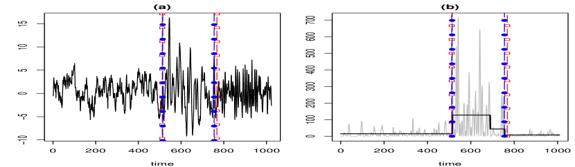
Figure 1: (a) A realisation of model (9) with true (empty square) and detected (filled circle) breakpoints; (b) $I^{(i)}_{t,T}$ at $i=-4$ and the breakpoint detection outcome.

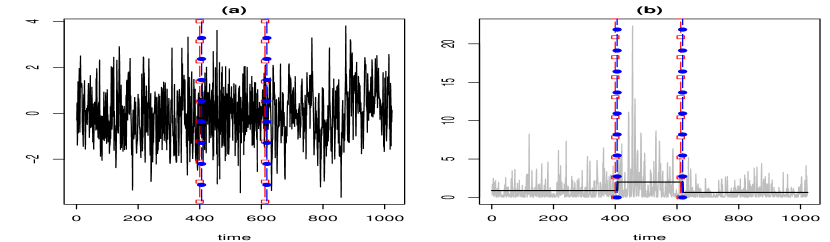
Figure 2: (a) A realisation of model (13); (b) $I^{(i)}_{t,T}$ at $i=-1$ and the breakpoint detection outcome.

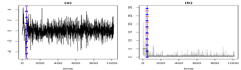
Figure 3: (a) A realisation of model (16); (b) $I^{(i)}_{t,T}$ at $i=-3$ and the breakpoint detection outcome.

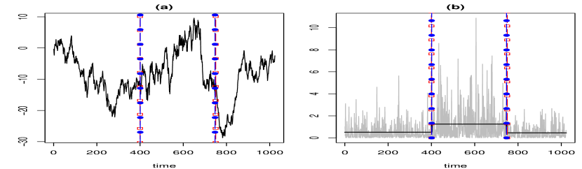
Figure 4: (a) A realisation of model (20); (b) $I^{(i)}_{t,T}$ at $i=-1$ and the breakpoint detection outcome.

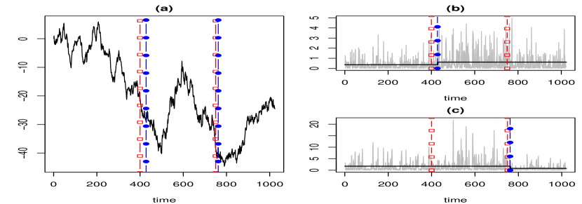
Figure 5: (a) A realisation of model (24); (b) $I^{(i)}_{t,T}$ at $i=-1$ and the breakpoint detection outcome; (c) $I^{(i)}_{t,T}$ at $i=-2$ and the breakpoint detection outcome.

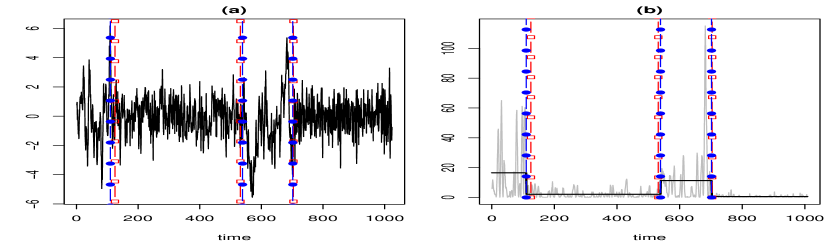
Figure 6: (a) A realisation of model (29); (b) $I^{(i)}_{t,T}$ at $i=-4$ and the breakpoint detection outcome.

Table 2: Summary of breakpoint detection from Simulation (A): our method (CF) and Auto-PARM (AP). Results over $100$ simulations.

number of breakpoints
a	0.7		0.4		0.1		-0.1		-0.4		-0.7
	CF	AP	CF	AP	CF	AP	CF	AP	CF	AP	CF	AP
0	100	100	100	100	100	100	99	100	99	100	94	100
1	0	0	0	0	0	0	1	0	1	0	5	0
$\geq$ 2	0	0	0	0	0	0	0	0	0	0	1	0
total	100	100	100	100	100	100	100	100	100	100	100	100

Table 3: Summary of breakpoint detection from simulations: our method (CF) and Auto-PARM (AP). Results over $100$ simulations.

number of breakpoints
	model (B)		model (C)		model (D)		model (E)		model (F)		model (G)
	CF	AP	CF	AP	CF	AP	CF	AP	CF	AP	CF	AP
0	0	0	0	0	0	0	1	42	1	20	0	0
1	0	0	0	0	97	100	0	31	14	68	1	16
2	93	99	96	100	3	0	97	16	84	7	6	55
3	4	1	3	0	0	0	2	9	1	3	76	29
4	3	0	1	0	0	0	0	0	0	1	17	0
5	0	0	0	0	0	0	0	2	0	1	0	0
total	100	100	100	100	100	100	100	100	100	100	100	100

5 U.S stock market data analysis

Many authors, including Stărică and Granger (2005), argue in favour of nonstationary modelling of financial returns. In this analysis, we consider the Dow Jones Industrial Average index and regard it as a process with an extremely high degree of autocorrelation (such as in the near-unit-root model of Phillips and Perron (1988)) and a time-varying variance, similar to the simulation model in Section 4 (E).

(A) Dow Jones weekly closing values 1970–1975

The time series of weekly closing values of the Dow Jones Industrial Average index between July 1971 and August 1974 was studied in Hsu (1979) and revisited in Chen and Gupta (1997). Historical data are available on www.google.com/finance/historical?q=INDEXDJX:.DJI, where daily and weekly prices can be extracted for any time period. Both papers concluded that there was a change in the variance of the index around the third week of March 1973. For ease of computation of the wavelet periodogram, we chose the same weekly index between 1 July 1970 and 19 May 1975 so that the data size was $T=256$ with the above-mentioned time period was contained in this interval. The third week of March 1973 corresponds to $t=141$ and our procedure detected $\widehat{\eta}=142$ as a breakpoint, as illustrated in Figure 8. The Auto-PARM did not return any breakpoint, while the segmentation procedure proposed in Lavielle and Teyssière (2005), when applied to the log-returns ($\log(X_{t}/X_{t-1})$) of the data rather than the data $X_{t}$ themselves, returned $t=141$ as a breakpoint, which is very close to $\widehat{\eta}$.

(B) Dow Jones daily closing values 2007–2009

We further investigated more recent daily data from the same source, between 8 January 2007 and 16 January 2009. Over this period, the global financial market experienced one of the worst crises in history. Our breakpoint detection algorithm found two breakpoints (see Figure 8), one in the last week of July 2007 ($\widehat{\eta}_{1}=135$), and the other in mid-September 2008 ($\widehat{\eta}_{2}=424$). The Auto-PARM returned three breakpoints on average, although the estimated breakpoints were unstable as in Section 4 (E): $t=35,426$ and $488$ were detected most often as breakpoints, while $t=100$ and $t=140$ were detected in place of $t=35$ on other occasions. The segmentation procedure from Lavielle and Teyssière (2005), when applied to the log-returns ($\log(X_{t}/X_{t-1})$) of the data rather than the data $X_{t}$ themselves, detected $t=127$ and $424$ as breakpoints, which are very close to $\widehat{\eta}_{1}$ and $\widehat{\eta}_{2}$. The first breakpoint coincided with the outbreak of the worldwide “credit crunch” as subprime mortgage-backed securities were discovered in portfolios of banks and hedge funds around the world. The second breakpoint coincided with the bankruptcy of Lehman Brothers, a major financial services firm, an event that brought even more volatility to the market. Evidence supporting our breakpoint detection outcome is the TED spread (available from http://www.bloomberg.com/apps/quote?ticker=.tedsp:ind), an indicator of perceived credit risk in the general economy; it spiked up in late July 2007, remained volatile for a year, then spiked even higher in September 2008. These movements coincide almost exactly with our detected breakpoints.

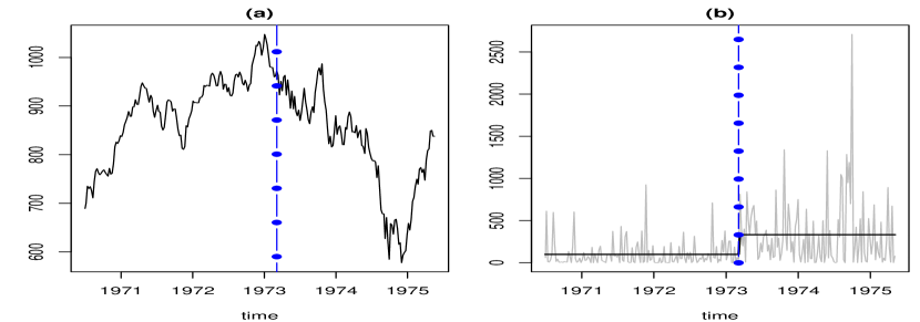
Figure 7: (a) Weekly average values of the Dow Jones IA index (July 1970–May 1975); (b) Wavelet periodogram at scale $-1$ and the breakpoint detection outcome.

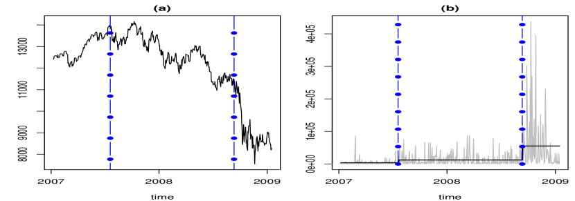
Figure 8: (a) Daily average values of the Dow Jones IA index (Jan 2007–Jan 2009); (b) Wavelet periodogram at scale $-1$ and the breakpoint detection outcome.

Appendix A The proof of Theorem 1

The consistency of our algorithm is first proved for the sequence below,

$$\widetilde{Y}^{2}_{t,T}=\sigma^{2}(t/T)\cdot Z^{2}_{t,T},\ t=0,\ldots,T-1.$$ (30)

Note that unlike in (3), the above model features the true piecewise constant $\sigma^{2}(t/T)$. Denote $n=e-s+1$ and define

$$\widetilde{\mathbb{Y}}^{b}_{s,e} = \frac{\sqrt{e-b}}{\sqrt{n}\sqrt{b-s+1}}\sum_{t=s}^{b}\widetilde{Y}^{2}_{t,T}-\frac{\sqrt{b-s+1}}{\sqrt{n}\sqrt{e-b}}\sum_{t=b+1}^{e}\widetilde{Y}^{2}_{t,T}.$$

$\widetilde{\mathbb{S}}^{b}_{s,e}$ and $\mathbb{S}^{b}_{s,e}$ are defined similarly, replacing $\widetilde{Y}^{2}_{t,T}$ with $\sigma^{2}(t/T)$ and $\sigma^{2}_{t,T}$, respectively. Note that the above are simply inner products of the respective sequences and a vector whose support starts at $s$, is constant and positive until $b$, then constant negative until $e$, and normalised such that it sums to zero and sums to one when squared. Let $s$, $e$ satisfy $\eta_{p_{0}}\leq s<\eta_{p_{0}+1}<\ldots<\eta_{p_{0}+q}<e\leq\eta_{p_{0}+q+1}$ for $0\leq p_{0}\leq B-q$, which will always be the case at all stages of the algorithm. In Lemmas 1–5 below, we impose at least one of following conditions:

$$s<\eta_{p_{0}+r}-C\delta_{T}<\eta_{p_{0}+r}+C\delta_{T}<e\mbox{ for some }1\leq r\leq q,$$ (31)

$$\{(\eta_{p_{0}+1}-s)\wedge(s-\eta_{p_{0}})\}\vee\{(\eta_{p_{0}+q+1}-e)\wedge(e-\eta_{p_{0}+q})\}\leq\epsilon_{T},$$ (32)

where $\wedge$ and $\vee$ are the minimum and maximum operators, respectively. We remark that both conditions (31) and (32) hold throughout the algorithm for all those segments starting at $s$ and ending at $e$ which contain previously undetected breakpoints. As Lemma 6 concerns the case when all breakpoint have already been detected, it does not use either of these conditions.

The proof of the theorem is constructed as follows. Lemma 1 is used in the proof of Lemma 2, which in turn is used alongside Lemma 3 in the proof of Lemma 4. From the result of Lemma 4, we derive Lemma 5 and finally, Lemmas 5 and 6 are used to prove Theorem 1.

Lemma 1.

Let $s$ and $e$ satisfy (31), then there exists $1\leq r^{*}\leq q$ such that

$$\left|\widetilde{\mathbb{S}}^{\eta_{p_{0}+r^{*}}}_{s,e}\right|=\max_{s<t<e}|\widetilde{\mathbb{S}}^{t}_{s,e}|\geq C\delta_{T}/\sqrt{T}.$$ (33)

Proof. The equality in (33) is proved by Lemmas 2.2 and 2.3 of Venkatraman (1993). For the inequality part, we note that in the case of a single breakpoint in $\sigma^{2}(z)$, $r$ in (31) coincides with $r^{*}$ and we can use the constancy of $\sigma^{2}(z)$ to the left and to the right of the breakpoint to show that

$$\left|\widetilde{\mathbb{S}}^{\eta_{p_{0}+r}}_{s,e}\right|=\left|\frac{\sqrt{\eta_{p_{0}+r}-s+1}\sqrt{e-\eta_{p_{0}+r}}}{\sqrt{n}}\left(\sigma^{2}(\eta_{p_{0}+r}/T)-\sigma^{2}((\eta_{p_{0}+r}+1)/T)\right)\right|,$$

which is bounded from below by $C\delta_{T}/\sqrt{T}$. In the case of multiple breakpoints, we remark that for any $r$ satisfying (31), the above order remains the same and thus (33) follows. $\square$

Lemma 2.

Suppose (31) holds, and let $\eta\equiv\eta_{p_{0}+r}\in[s,e]$ for some $r\in\{1,\ldots,q\}$, denote a true change-point. Then there exists $c_{0}\in(0,\infty)$ such that for $b$ satisfying $|\widetilde{\mathbb{S}}_{s,e}^{b}|<|\widetilde{\mathbb{S}}_{s,e}^{\eta}|$ and $|\eta-b|\geq c_{0}\epsilon_{T}$ with $\epsilon_{T}=T^{5/2-2\Theta}\log\,T$, we have $|\widetilde{\mathbb{S}}_{s,e}^{\eta}|-|\widetilde{\mathbb{S}}_{s,e}^{b}|\geq 2\log\,T$.

Proof. Let both $\widetilde{\mathbb{S}}_{s,e}^{\eta}$, $\widetilde{\mathbb{S}}_{s,e}^{b}$ $\geq 0$ without loss of generality.

The proof follows directly from the proof of Lemma 2.6 in Venkatraman (1993). We only consider Case 2 of Lemma 2.6, since adapting the proof of Case 1 (when there is a single change-point within $[s,e]$) to that of the current lemma takes analogous arguments.

Using the notations therein, it is shown that the term $E_{1l}$ is dominant over $E_{2l}$ and $E_{3l}$ in $\widetilde{\mathbb{S}}_{s,e}^{\eta}-\widetilde{\mathbb{S}}_{s,e}^{b}$, where $l=c_{0}\epsilon_{T}$. Noting further that $i=\eta-s+1$, $h=\delta_{T}$, $j=e-\eta-h$ and $a=\sum_{t=s}^{\eta}\sigma^{2}(t/T)-(e-s+1)^{-1}\sum_{t=s}^{e}\sigma^{2}(t/T)$, and that $h\geq 2l$,

$$E_{1l} = \frac{la\sqrt{i+j+h}}{\sqrt{i}\sqrt{j+h}}\cdot\frac{h-l}{\sqrt{i+l}\sqrt{j+h-l}\{\sqrt{(i+l)(j+h-l)}+\sqrt{i(j+l)}\}}$$

$$\geq \widetilde{\mathbb{S}}_{s,e}^{\eta}\cdot C\epsilon_{T}\delta_{T}T^{-2}\geq 2\log\,T$$

for large $T$. $\square$

Lemma 3.

$\left|\widetilde{\mathbb{Y}}^{b}_{s,e}-\widetilde{\mathbb{S}}^{b}_{s,e}\right|\leq\log T$ with probability converging to $1$ with $T$ uniformly over $(s,b,e)\in\mathcal{D}$, where, for $c\in(0,\infty)$,

$$\mathcal{D}:=\left\{1\leq s<b<e\leq T;\ e-s+1\geq C\delta_{T},\ \max\left\{\sqrt{\frac{b-s+1}{e-b}},\sqrt{\frac{e-b}{s-b+1}}\right\}\leq c\right\}.$$

Proof. We need to show that

$$\mathbf{P}\left(\max_{(s,b,e)\in\mathcal{D}}\frac{1}{\sqrt{n}}\left|\sum_{t=s}^{e}\sigma^{2}(t/T)(Z^{2}_{t,T}-1)\cdot c_{t}\right|>\log T\right)\longrightarrow 0,$$ (34)

where $c_{t}=\sqrt{e-b}/\sqrt{b-s+1}$ for $t\in[s,b]$ and $c_{t}=\sqrt{b-s+1}/\sqrt{e-b}$ otherwise. Let $\{U_{t}\}_{t=s}^{e}$ be i.i.d. standard normal variables, $\mathbf{V}=(v_{i,j})_{i,j=1}^{n}$ with $v_{i,j}=\mbox{cor}\left(Z_{i,T},Z_{j,T}\right)$, and $\mathbf{W}=(w_{i,j})_{i,j=1}^{n}$ be a diagonal matrix with $w_{i,i}=\sigma^{2}(t/T)\cdot c_{t}$ where $i=t-s+1$. By standard results (see e.g. Johnson and Kotz (1970), page 151), showing (34) is equivalent to showing that $\left|\sum_{t=s}^{e}\lambda_{t-s+1}(U_{t}^{2}-1)\right|$ is bounded by $\sqrt{n}\log T$ with probability converging to 1, where $\lambda_{i}$ are eigenvalues of the matrix $\mathbf{VW}$. Due to the Gaussianity of $U_{t}$, $\lambda_{t-s+1}(U_{t}^{2}-1)$ satisfy the Cramér’s condition, i.e., there exists a constant $C>0$ such that

$$\mathbb{E}\left|\lambda_{t-s+1}(U_{t}^{2}-1)\right|^{p}\leq C^{p-2}p!\mathbb{E}\left|\lambda_{t-s+1}(U_{t}^{2}-1)\right|^{2},\ p=3,4,\ldots.$$

Therefore we can apply Bernstein’s inequality (Bosq 1998) and obtain

$$\mathbf{P}\left(\left|\sum_{t=s}^{e}\sigma^{2}(t/T)(Z^{2}_{t,T}-1)\cdot c_{t}\right|>\sqrt{n}\log T\right)\leq 2\exp\left(-\frac{n\log^{2}T}{4\sum_{i=1}^{n}\lambda_{i}^{2}+2\max_{i}|\lambda_{i}|C\sqrt{n}\log T}\right).$$

Note that $\sum_{i=1}^{n}\lambda_{i}^{2}=\mbox{tr}\left(\mathbf{VW}\right)^{2}\leq c^{2}\max_{z}\sigma^{4}(z)n\rho_{\infty}^{2}.$ Also it follows that $\max_{i}|\lambda_{i}|\leq c\max_{z}$ $\sigma^{2}(z)\|\mathbf{V}\|$ where $\|\cdot\|$ denotes the spectral norm of a matrix, and $\|\mathbf{V}\|\leq\rho^{1}_{\infty}$ since $\mathbf{V}$ is non-negative definite. Then (34) is bounded by

$$\sum_{(s,b,e)\in\mathcal{D}}2\exp\left(-\frac{n\log^{2}T}{4c^{2}\max_{z}\sigma^{4}(z)n\rho_{\infty}^{2}+2c\max_{z}\sigma^{2}(z)\sqrt{n}\log T\rho^{1}_{\infty}}\right)$$

$$\leq 2T^{3}\exp\left(-C\log^{2}T\right)\rightarrow 0,$$

as $\rho_{\infty}^{p}\leq C2^{I^{*}}$, which can be made to be of order $\log T$, since the only requirement on $I^{*}$ is that it converges to infinity but no particular speed is required. Thus the lemma follows. $\square$

Lemma 4.

Assume (31) and (32). For $b=\arg\max_{s<t<e}|\widetilde{\mathbb{Y}}^{t}_{s,e}|$, there exists $1\leq r\leq q$ such that $|b-\eta_{p_{0}+r}|\leq C\epsilon_{T}$ for a large $T$.

Proof. Let $\widetilde{\mathbb{S}}_{s,e}=\max_{s<t<e}|\widetilde{\mathbb{S}}^{t}_{s,e}|$. From Lemma 3, $\widetilde{\mathbb{Y}}^{b}_{s,e}\geq\widetilde{\mathbb{S}}_{s,e}-\log T$ and $\widetilde{\mathbb{S}}^{b}_{s,e}\geq\widetilde{\mathbb{Y}}^{b}_{s,e}-\log T$, hence $\widetilde{\mathbb{S}}^{b}_{s,e}\geq\widetilde{\mathbb{S}}_{s,e}-2\log T$. Assume that $|b-\eta_{p_{0}+r}|>C\epsilon_{T}$ for any $r$. From Lemma 2.2 in Venkatraman (1993), $\widetilde{\mathbb{S}}^{t}_{s,e}$ is either monotonic or decreasing and then increasing on $[\eta_{p_{0}+r},\eta_{p_{0}+r+1}]$ and $\widetilde{\mathbb{S}}^{\eta_{p_{0}+r}}_{s,e}\vee\widetilde{\mathbb{S}}^{\eta_{p_{0}+r+1}}_{s,e}>\widetilde{\mathbb{S}}^{b}_{s,e}$. Suppose that $\widetilde{\mathbb{S}}^{t}_{s,e}$ is decreasing and then increasing on the interval. Then from Lemma 2, we have $b^{\prime}=\eta_{p_{0}+r}+C\epsilon_{T}$ satisfying $\widetilde{\mathbb{S}}^{\eta_{p_{0}+r}}_{s,e}-2\log T\geq\widetilde{\mathbb{S}}^{b^{\prime}}_{s,e}$. Since $\widetilde{\mathbb{S}}^{t}_{s,e}$ is locally increasing at $t=b$ (for $\widetilde{\mathbb{S}}^{b}_{s,e}>\widetilde{\mathbb{S}}^{b^{\prime}}_{s,e}$), we have $\widetilde{\mathbb{S}}^{\eta_{p_{0}+r+1}}_{s,e}>\widetilde{\mathbb{S}}^{b}_{s,e}$ and there will again be a $b^{\prime\prime}=\eta_{p_{0}+r+1}-C\epsilon_{T}$ satisfying $\widetilde{\mathbb{S}}^{\eta_{p_{0}+r}}_{s,e}-2\log T\geq\widetilde{\mathbb{S}}^{b^{\prime\prime}}_{s,e}$. As $b^{\prime\prime}>b$, it contradicts that $\widetilde{\mathbb{S}}^{b}_{s,e}\geq\widetilde{\mathbb{S}}_{s,e}-2\log T$. Similar arguments are applicable when $\widetilde{\mathbb{S}}^{t}_{s,e}$ is monotonic and therefore the lemma follows. $\square$

Lemma 5.

Under (31) and (32), $\mathbf{P}\left(\left|\widetilde{\mathbb{Y}}^{b}_{s,e}\right|<\tau T^{\theta}\sqrt{\log T}\cdot n^{-1}\sum_{t=s}^{e}\widetilde{Y}^{2}_{t,T}\right)\longrightarrow 0$ for $b=\arg\max_{s<t<e}|\widetilde{\mathbb{Y}}^{t}_{s,e}|$.

Proof. From Lemma 4, there exists some $r$ such that $|b-\eta_{p_{0}+r}|<C\epsilon_{T}$. Denote $\widetilde{d}=\widetilde{\mathbb{Y}}^{b}_{s,e}=\widetilde{d}_{1}-\widetilde{d}_{2}$ and $\widetilde{m}=n^{-1/2}\sum_{t=s}^{e}\widetilde{Y}^{2}_{t,T}=c_{1}\widetilde{d}_{1}+c_{2}\widetilde{d}_{2}$, where

$$\widetilde{d}_{1}=\frac{\sqrt{e-b}}{\sqrt{n}\sqrt{b-s+1}}\sum_{t=s}^{b}\widetilde{Y}^{2}_{t,T},\ \ \widetilde{d}_{2}=\frac{\sqrt{b-s+1}}{\sqrt{n}\sqrt{e-b}}\sum_{t=b+1}^{e}\widetilde{Y}^{2}_{t,T},\ \mbox{ and}\ c_{1}=c_{2}^{-1}=\sqrt{\frac{b-s+1}{e-b}}.$$

For simplicity, let $c_{2}>c_{1}$. Further, let $\mu_{i}=\mathbb{E}\widetilde{d}_{i}$ and $w_{i}=\mbox{var}(\widetilde{d}_{i})$ for $i=1,2$, and define $\mu=\mathbb{E}\widetilde{d}$ and $w=\mbox{var}(\widetilde{d})$. Finally, $\mathit{t}_{n}$ denotes the threshold $\tau T^{\theta}\sqrt{\log T/n}$. We need to show $\mathbf{P}(|\widetilde{d}|\leq\widetilde{m}\cdot\mathit{t}_{n})\rightarrow 0.$ Note that $w_{i}\leq c^{2}\sup_{z}\sigma^{4}(z)\rho^{2}_{\infty}$. Using Markov’s and the Cauchy-Schwarz inequalities, we bound $\mathbf{P}(\widetilde{d}\leq\widetilde{m}\cdot\mathit{t}_{n})$ by

$$\mathbf{P}\left\{(\widetilde{d}_{1}-\mu_{1})(c_{1}\mathit{t}_{n}-1)+(\widetilde{d}_{2}-\mu_{2})(c_{2}\mathit{t}_{n}+1)+2c_{1}\mathit{t}_{n}\mu_{1}+(c_{2}-c_{1})\mathit{t}_{n}\mu_{2}\geq(1+c_{1}\mathit{t}_{n})\mu\right\}$$

$$\leq 4\mu^{-2}(1+c_{1}\mathit{t}_{n})^{-2}\left\{(c_{1}\mathit{t}_{n}-1)^{2}w_{1}+(c_{2}\mathit{t}_{n}+1)^{2}\widetilde{+}4c_{1}^{2}\mathit{t}_{n}^{2}\mu_{1}^{2}+(c_{2}-c_{1})^{2}\mathit{t}_{n}^{2}\mu_{2}^{2}\right\}$$

$$\leq O\left\{\mu^{-2}\sup_{z}\sigma^{4}(z)\left(\rho^{2}_{\infty}+\tau^{2}T^{2\theta}\log T\right)\right\},$$

and since $\mu=\widetilde{\mathbb{S}}^{b}_{s,e}=O\left(\delta_{T}/\sqrt{T}\right)>T^{\theta}\sqrt{\log T},$ the conclusion follows. $\square$

Lemma 6.

For some positive constants $C,\ C^{\prime}$, let $s$, $e$ satisfy either

• $\exists\,1\leq p\leq B$ such that $s\leq\eta_{p}\leq e$ and $[\eta_{p}-s+1]\wedge[e-\eta_{p}]\leq C\epsilon_{T}$  or

• $\exists\,1\leq p\leq B$ such that $s\leq\eta_{p}<\eta_{p+1}\leq e$ and $[\eta_{p}-s+1]\vee[e-\eta_{p+1}]\leq C^{\prime}\epsilon_{T}$.

Then for a large $T$,

$$\mathbf{P}\left(\left|\widetilde{\mathbb{Y}}^{b}_{s,e}\right|>\tau T^{\theta}\sqrt{\log T}\cdot n^{-1}\sum_{t=s}^{e}\widetilde{Y}^{2}_{t,T}\right)\longrightarrow 0,$$

where $b=\arg\max_{s<t<e}|\widetilde{\mathbb{Y}}^{t}_{s,e}|$.

Proof. First we assume (i). Let $\mathcal{A}=\left\{\left|\widetilde{\mathbb{Y}}^{b}_{s,e}\right|>\tau T^{\theta}\sqrt{\log T}\cdot n^{-1}\sum_{t=s}^{e}\widetilde{Y}^{2}_{t,T}\right\}$ and

$$\mathcal{B}=\left\{\frac{1}{n}\left|\sum_{t=s}^{e}\left(\widetilde{Y}^{2}_{t,T}-\mathbb{E}\widetilde{Y}^{2}_{t,T}\right)\right|<h=\frac{(\eta_{p}-s+1)\sigma^{2}_{1}+(e-\eta_{p})\sigma^{2}_{2}}{2n}\right\},$$

where $\sigma^{2}_{1}=\sigma^{2}\left(\eta_{p}/T\right)$ and $\sigma^{2}_{2}=\sigma^{2}\left((\eta_{p}+1)/T\right)$. We have $\mathbf{P}\left(\mathcal{A}\right)=\mathbf{P}\left(\mathcal{A}\cap\mathcal{B}\right)+\mathbf{P}\left(\mathcal{A}\left|\mathcal{B}^{c}\right.\right)\mathbf{P}\left(\mathcal{B}^{c}\right)\leq\mathbf{P}\left(\mathcal{A}\cap\mathcal{B}\right)+\mathbf{P}\left(\mathcal{B}^{c}\right).$ The first part is bounded as

$$\mathbf{P}\left(\mathcal{A}\cap\mathcal{B}\right)\leq\mathbf{P}\left(\left|\widetilde{\mathbb{Y}}^{b}_{s,e}\right|>\tau T^{\theta}\sqrt{\log T}\cdot n^{-1}\sum_{t=s}^{e}\left(\mathbb{E}\widetilde{Y}^{2}_{t,T}-h\right)\right).$$ (35)

From Lemma 3, we have $|\widetilde{\mathbb{Y}}_{s,e}^{b}-\widetilde{\mathbb{S}}_{s,e}^{b}|\leq\log T$. Also Lemmas 2.2 and 2.3 of Venkatraman (1993) indicate that $\max_{s<t<e}|\widetilde{\mathbb{S}}^{t}_{s,e}|=|\widetilde{\mathbb{S}}^{\eta_{p}}|=O(\sqrt{n^{-1}\epsilon_{T}(n-C\epsilon_{T})})=O(\sqrt{\epsilon_{T}})$. Therefore $|\widetilde{\mathbb{Y}}_{s,e}^{b}|\leq|\widetilde{\mathbb{S}}^{\eta_{p}}|+\log T=O(\sqrt{\epsilon_{T}})$ and (35) is bounded by $\mathbb{E}\left(\widetilde{\mathbb{Y}}_{s,e}^{b}\right)^{2}/(\tau^{2}h^{2}T^{2\theta}\log T)\leq O\left(T^{1/2-2\theta}\right)\longrightarrow 0,$ by applying Markov’s inequality. Turning our attention to $\mathbf{P}\left(\mathcal{B}^{c}\right)$, we need to show that

$$\mathbf{P}\left(\frac{1}{n}\left|\sum_{t=s}^{e}\sigma^{2}(t/T)(Z^{2}_{t,T}-1)\right|>h\right)\longrightarrow 0.$$

This can be shown by applying Bernstein’s inequality as in the proof of Lemma 3, and the lemma follows. Similar arguments are applied when (ii) holds. $\square$

We now prove Theorem 1. At the start of the algorithm, as $s=0$ and $e=T-1$, all conditions for Lemma 5 are met and it finds a breakpoint within the distance of $C\epsilon_{T}$ from the true breakpoint, by Lemma 4. Under Assumption 2, both (31) and (32) are satisfied within each segment until every breakpoint in $\sigma^{2}(t/T)$ is identified. Then, either of two conditions (i) or (ii) in Lemma 6 is met and therefore no further breakpoint is detected with probability converging to 1.

Next we study how the bias present in $\mathbb{E}I^{(i)}_{t,T}(=\sigma^{2}_{t,T})$ affects the consistency. First we define the autocorrelation wavelet $\Psi_{i}(\tau)=\sum_{k=-\infty}^{\infty}\psi_{i,k}\psi_{i,k+\tau}$, the autocorrelation wavelet inner product matrix $A_{i,j}=\sum_{\tau}\Psi_{i}(\tau)\Psi_{j}(\tau)$, and the across-scales autocorrelation wavelets $\Psi_{i,j}(\tau)=\sum_{k}\psi_{i,k}\psi_{j,k+\tau}$. Then it is shown in Fryzlewicz and Nason (2006) that the integrated bias between $\mathbb{E}I^{(i)}_{t,T}$ and $\beta_{i}(t/T)$ converges to zero.

Proposition 1 (Propositions 2.1-2.2 (Fryzlewicz and Nason 2006)).

Let $I^{(i)}_{t,T}$ be the wavelet periodogram at a fixed scale $i$. Under Assumption 1,

$$T^{-1}\sum_{t=0}^{T-1}\left|\mathbb{E}I^{(i)}_{t,T}-\beta_{i}(t/T)\right|^{2}=O(T^{-1}2^{-i})+b_{i,T},$$ (36)

where $b_{i,T}$ depends on the sequence $\{L_{i}\}_{i}$. Further, each $\beta_{i}(z)$ is a piecewise constant function with at most $B$ jumps, all of which occur in the set $\mathcal{B}$.

Suppose the interval $[s,e]$ includes a true breakpoint $\eta_{p}$ as in (31), and denote $b=\arg\max_{t\in(s,e)}|\widetilde{\mathbb{S}}^{t}_{s,e}|$ and $\widehat{b}=\arg\max_{t\in(s,e)}\left|\mathbb{S}^{t}_{s,e}\right|$. Recall that $\mathbb{E}I^{(i)}_{t,T}$ remains constant within each stationary segment, apart from short (of length $C2^{-i}$) intervals around the discontinuities in $\beta_{i}(t/T)$. Suppose a jump occurs at $\eta_{p}$ in $\beta_{i}(t/T)$ yet there is no change in $\mathbb{E}I^{(i)}_{t,T}$ for $t\in[\eta_{p}-C2^{-i},\eta_{p}+C2^{-i}]$. Then the integrated bias is bounded from below by $C\delta_{T}/T$ from Assumption 2, and Proposition 1 is violated. Therefore there will be a change in $\mathbb{E}I^{(i)}_{t,T}$ as well on such intervals around $\eta_{p}$ and $\mathbb{E}I^{(i)}_{t_{1},T}\neq\mathbb{E}I^{(i)}_{t_{2},T}$ for $t_{1}\leq\eta_{p}-C2^{-i}$ and $t_{2}\geq\eta_{p}+C2^{-i}$. Although the bias of $\mathbb{E}I^{(i)}_{t,T}$ in relation to $\beta_{i}(t/T)$ may cause some bias between $\widehat{b}$ and $b$, we have that $|\widehat{b}-b|\leq C2^{I^{*}}<\epsilon_{T}$ holds for $I^{*}=O(\log\log T)$, which is an admissible rate for $I^{*}$. Besides, once one breakpoint is detected in such intervals, the algorithm does not allow any more breakpoints to be detected within the distance of $\Delta_{T}$ from the detected breakpoint, by construction. Hence the bias in $\mathbb{E}I^{(i)}_{t,T}$ does not affect the results of Lemmas 1–6 for wavelet periodograms at finer scales and the consistency still holds for $Y^{2}_{t,T}$ in (3).

Finally, we note that the within-scale post-processing step in Section 3.2.1 is in line with the theoretical consistency of our procedure; (a) Lemma 5 implies that our test statistic exceeds the threshold when there is a breakpoint $\eta$ within a segment $[s,e]$ which is of sufficient distance from both $s$ and $e$, and (b) Lemma 6 shows that it does not exceed the threshold when $(s,\eta,e)$ does not satisfy the condition in (a).

Appendix B The proof of Theorem 2

From Assumption 1 and the invertibility of the autocorrelation wavelet inner product matrix $A$, there exists at least one sequence of wavelet periodograms among $I^{(i)}_{t,T},\ i=-1,\ldots,-I^{*}$ in which any breakpoint in $\mathcal{B}$ is detected. Suppose there is only one such scale, $i_{0}$, for $\nu_{q}\in\mathcal{B}$ and denote the detected breakpoint as $\widehat{\eta}^{(i_{0})}_{p_{0}}$. After the across-scales post-processing, $\widehat{\eta}^{(i_{0})}_{p_{0}}$ is selected as $\widehat{\nu}_{q}$ since no other $\widehat{\eta}^{(i)}_{p}$, $i\neq i_{0}$, is within the distance of $\Lambda_{T}=C\epsilon_{T}$ from either $\widehat{\nu}_{q}$ or $\widehat{\eta}^{(i_{0})}_{p_{0}}$, and $\left|\nu_{q}-\widehat{\eta}^{(i_{0})}_{p_{0}}\right|\leq\epsilon_{T}$ with probability converging to 1 from Theorem 1. If there are $D(\leq I^{*})$ breakpoints detected for $\nu_{q}$, denote them as $\widehat{\eta}^{(i_{1})}_{p_{1}},\ldots,\widehat{\eta}^{(i_{D})}_{p_{D}}$. Then for any $1\leq a<b\leq D$, $\left|\widehat{\eta}^{(i_{a})}_{p_{a}}-\widehat{\eta}^{(i_{b})}_{p_{b}}\right|\leq\left|\widehat{\eta}^{(i_{a})}_{p_{a}}-\nu_{q}\right|+\left|\widehat{\eta}^{(i_{b})}_{p_{b}}-\nu_{q}\right|\leq C\epsilon_{T},$ and only the one from the finest scale is selected as $\widehat{\nu}_{q}$ among them by the post-processing procedure. Hence the across-scales post-processing preserves the consistency for the breakpoints selected as its outcome.

References

- (1)
- Adak (1998) Adak, S. (1998). Time-dependent spectral analysis of nonstationary time series. Journal of the American Statistical Association. 93, 1488–1501.
- Andreou and Ghysels (2002) Andreou, E. and Ghysels, E. (2002). Detecting multiple breaks in financial market volatility dynamics. Journal of Applied Economics. 17, 579–600.
- Bai and Perron (1998) Bai, J. and Perron, P. (1998). Estimating and testing linear models with multiple structural changes. Econometrica. 66, 47–78.
- Bosq (1998) Bosq, D. (1998). Nonparametric statistics for stochastic process: estimation and prediction. Springer.
- Chen and Gupta (1997) Chen, J. and Gupta, A. K. (1997). Testing and locating variance change-points with application to stock prices. Journal of the American Statistical Association. 92, 739–747.
- Chernoff and Zacks (1964) Chernoff, H. and Zacks, S. (1964). Estimating the current mean of a normal distribution which is subject to changes in time. Annals of Mathematical Statistics. 35, 999–1028.
- Davis et al. (2006) Davis, R. A., Lee, T. C. M., and Rodriguez-Yam, G. A. (2006). Structural break estimation for non-stationary time series. Journal of the American Statistical Association. 101, 223–239.
- Davis et al. (2008) Davis, R. A., Lee, T. C. M., and Rodriguez-Yam, G. A. (2008). Break detection for a class of nonlinear time series models. Journal of Time Analysis. 29, 834–867.