Non-perturbative running of quark masses in three-flavour QCD

I. Campos,a,b P. Fritzsch,b,d C. Pena,b,c ,bA. Ramos,d and A. Vladikase
a Instituto de Física de Cantabria - IFCA-CSIC,
Avda. de Los Castros s/n, 39005 Santander, Spain
b Instituto de Física Teórica UAM/CSIC, Universidad Autónoma de Madrid,
C/ Nicolás Cabrera 13-15, Cantoblanco, Madrid 28049
c Departamento de Física Teórica, Universidad Autónoma de Madrid,
Cantoblanco, Madrid 28049
d Theoretical Physics Department, CERN,
CH-1211 Geneva 23, Switzerland
e INFN, Sezione di Tor Vergata, c/o Dipartimento di Fisica, Universitá di Roma Tor Vergata,
Via della Ricerca Scientifica 1, I-00133 Rome, Italy
E-mail
Abstract:

We present our preliminary results for the computation of the non-perturbative running of renormalized quark masses in $N_{f}=3$ QCD, between the electroweak and hadronic scales, using standard finite-size scaling techniques. The computation is carried out to very high precision, using massless $\mathcal{O}(a)$ improved Wilson quarks. Following the strategy adopted by the ALPHA Collaboration for the running coupling, different schemes are used above and below a scale $\mu_{0}\sim m_{b}$, which differ by using either the Schr dinger Functional or Gradient Flow renormalized coupling. We discuss our results for the running in both regions, and the procedure to match the two schemes.

Refer to caption
Refer to caption
Figure 1: The plots show the SSFs in both SF and GF coupling regions with respectively blue and red points (the two most hadronic points have not been used in the current analysis). The error bands coming from fitting $\sigma_{P}$ and $\tau$ are laying on top of each others showing a remarkable agreement between the two fitting procedures. The comparison with the LO and NLO is also provided (the latter is known only in the SF coupling region).

1 Introduction

The high precision computation of quark masses requires to control the Renormalization Group (RG) running very accurately and in a large range of scales. The equations describing the RG flow in a mass-independent scheme for the renormalized coupling $\bar{g}(\mu)$ and the renormalized mass $\bar{m}(\mu)$ respectively read

$\displaystyle\mu\frac{\partial}{\partial\mu}\bar{g}(\mu)$ $\displaystyle=\beta(\bar{g}(\mu))\,,$ (1)
$\displaystyle\mu\frac{\partial}{\partial\mu}\bar{m}(\mu)$ $\displaystyle=\tau(\bar{g}(\mu))\bar{m}(\mu)\,.$ (2)

They admit perturbative expansion

$\displaystyle\beta(g)$ $\displaystyle\stackrel{{\scriptstyle g\to 0}}{{\sim}}-g^{3}(b_{0}+b_{1}g^{2}+b_{2}g^{4}+\mathcal{O}(g^{6}))\,,$ (3)
$\displaystyle\tau(g)$ $\displaystyle\stackrel{{\scriptstyle g\to 0}}{{\sim}}-g^{2}(d_{0}+d_{1}g^{2}+d_{2}g^{4}+\mathcal{O}(g^{6}))\,,$ (4)

with universal coefficients $b_{0}$, $b_{1}$, $d_{0}$, while all the others are scheme-dependent. We can also define through formal solution of (1), (2) the renormalization group invariants (RGI) for both coupling and mass (the latter is valid for any multiplicatively renormalizable composite operator [1]) respectively as

$\displaystyle\Lambda$ $\displaystyle=\mu\left[b_{0}\bar{g}^{2}(\mu)\right]^{-b_{1}/(2b_{0}^{2})}e^{-1/(2b_{0}\bar{g}^{2}(\mu))}\exp\left\{-\int_{0}^{\bar{g}(\mu)}\,dg\,\left[\frac{1}{\beta(g)}+\frac{1}{b_{0}g^{3}}-\frac{b_{1}}{b_{0}^{2}g}\right]\right\}\,,$ (5)
$\displaystyle M$ $\displaystyle=\bar{m}(\mu)\left[2b_{0}\bar{g}^{2}(\mu)\right]^{-d_{0}/(2b_{0})}\exp\left\{-\int_{0}^{\bar{g}(\mu)}\,dg\,\left[\frac{\tau(g)}{\beta(g)}-\frac{d_{0}}{b_{0}g}\right]\right\}.$ (6)

In order to compute the running over several orders of magnitude we use a recursive procedure in finite volume with Schrödinger Functional (SF) [2] boundary conditions and massless, non-perturbatively $\mathcal{O}(a)$-improved Wilson fermions. Following the standard SF approach we identify the scale as the inverse box size $\mu=1/L$ and through a recursive fine-size scaling $L\to sL$ in the continuum it is possible to compute the running from large volume simulations ($L\sim 1/\Lambda_{QCD}$) up to the high energy regions ($L\sim 1/M_{W}$) where perturbation theory is well defined and can be safely applied.

2 Step Scaling Functions and SF Renormalization Conditions

Refer to caption
Refer to caption
Refer to caption
Figure 2: Continuum extrapolations of $\Sigma_{P}(u)$ for the three values of $u_{SF}$ reported in these proceedings. Blue (red) points are raw (1-loop improved [3]) SSFs. The limit $a\to 0$ is approached quadratically in $a/L$ according to [4].

In our computation the renormalization group functions are accessed through the Step Scaling Functions (SSFs) $\sigma$ and $\sigma_{P}$ defining the scale evolution of a factor $s>1$ for the coupling and the quark mass respectively as

$\displaystyle-\ln(s)$ $\displaystyle=\int_{\sqrt{\bar{g}^{2}(\mu)}}^{\sqrt{\bar{g}^{2}(\mu/s)}}\,\frac{dg}{\beta(g)}\,,\quad\text{with}\quad\sigma(s,\bar{g}^{2}(\mu))=\bar{g}^{2}(\mu/s)\,,$ (7)
$\displaystyle\sigma_{P}(s,\bar{g}^{2}(\mu))$ $\displaystyle=\frac{\bar{m}(\mu)}{\bar{m}(\mu/s)}=\exp\left\{-\int_{\sqrt{\bar{g}^{2}(\mu)}}^{\sqrt{\bar{g}^{2}(\mu/s)}}\,\frac{\tau(g)}{\beta(g)}dg\right\}\,.$ (8)

In order to compute (8) on the lattice, we identify the renormalization pattern for the quark masses through the (non-singlet) axial Ward identity ($i\neq j$)

$\displaystyle\partial_{\mu}(A_{R})^{ij}_{\mu}$ $\displaystyle=(\bar{m}_{i}+\bar{m}_{j})P^{ij}_{R}\,.$ (9)

The renormalized currents are given by

$\displaystyle(A_{R})^{ij}_{\mu}(x)$ $\displaystyle=Z_{A}\bar{\psi}_{i}(x)\gamma_{\mu}\gamma_{5}\psi_{j}(x)\,,\quad(P_{R})^{ij}_{\mu}(x)=Z_{P}\bar{\psi}_{i}(x)\gamma_{5}\psi_{j}(x)\,,$ (10)

where $i,j$ are flavour indices. With $Z_{A}$ being finite, all the scale dependence of the mass is given by the inverse of the pseudoscalar renormalization constant $Z_{P}\propto 1/Z_{m}$. The renormalization constant $Z_{P}$ is computed from standard boundary-to-bulk and boundary-to-boundary correlation functions in the SF [5] by the renormalization condition

$\displaystyle\left.Z_{P}(g_{0},L/a)\frac{f_{P}(L/2)}{\sqrt{3f_{1}}}\right|^{\theta}_{m_{q}=0}$ $\displaystyle=c_{3}(\theta,a/L)\,,$ $\displaystyle\theta$ $\displaystyle=0.5\,,$ (11)

where $c_{3}$ is the tree-level normalisation and $\theta$ is entering in the definition of the boundary quark fields. In particular, the correlation functions in Eq. (11) are computed with vanishing background gauge field and quark masses and read

$\displaystyle f_{P}(x_{0})$ $\displaystyle=-\frac{1}{3}\int d^{3}\mathbf{y}\,d^{3}\,\mathbf{z}\;\left\langle\bar{\psi}(x)\gamma_{5}\frac{1}{2}\tau^{a}\psi(x)\bar{\zeta}(\mathbf{y})\gamma_{5}\frac{1}{2}\tau^{a}\zeta(\mathbf{z})\right\rangle\,,$ (12)
$\displaystyle f_{1}$ $\displaystyle=-\frac{1}{3L^{6}}\int d^{3}\mathbf{u}\,d^{3}\mathbf{v}\,d^{3}\mathbf{y}\,d^{3}\mathbf{z}\;\left\langle\bar{\zeta}^{\prime}(\mathbf{u})\gamma_{5}\frac{1}{2}\tau^{a}\zeta^{\prime}(\mathbf{v})\bar{\zeta}(\mathbf{y})\gamma_{5}\frac{1}{2}\tau^{a}\zeta(\mathbf{z})\right\rangle\,,$ (13)

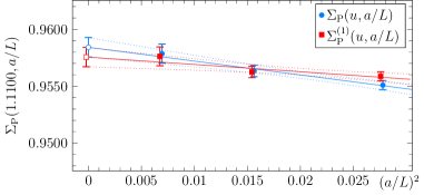
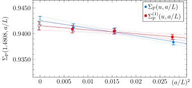
using the same notation as in [4]. The discrete version of (8) for $s=2$ is then given by

$\displaystyle\Sigma_{P}(u,a/L)$ $\displaystyle=\left.\frac{Z_{P}(g_{0},2L/a)}{Z_{P}(g_{0},L/a)}\right|_{u=\bar{g}^{2}(L)}$ (14)

from which the continuum limit $\sigma_{P}(u)=\lim_{a\to 0}\Sigma_{P}(u,a/L)$ can be taken. The results for $Z_{P}$ and $\Sigma_{P}$ are listed in Tab. 1. It has been observed [6, 7, 8] that the computational cost of measuring the SF coupling grows fast at low energies and in particular towards the continuum limit, thus it is challenging to reach the low energy domain characteristic for hadronic physics, especially if one aims at maintaining an high precision. The Gradient Flow (GF) coupling seems to be better suited for this task [9, 10, 11]. The relative precision of the coupling in this scheme is typically high and shows a weak dependence on both the energy scale and the cutoff. Following the same strategy employed by the ALPHA Collaboration for the computation of the running of the strong coupling [12, 11], we identify two energy regions $L>L_{0}$ and $L<L_{0}$, where the ”switching scale” between the two schemes $L_{0}\sim 1/m_{b}$ is defined by $\bar{g}^{2}_{SF}(L_{0})=2.012$, corresponding to $\bar{g}^{2}_{GF}(2L_{0})=2.6723(64)$. Note that, as part of the renormalization condition for the mass, the value of the renormalized coupling is specified. Therefore, using a different renormalized coupling (e.g. GF or SF) results in a different renormalization scheme for the mass [3]. In the current project we have performed a NP computation of the SSF for $u_{SF}=[1.1100,1.1844,1.2565,1.3627,1.4808,1.6173,1.7943,2.0120]$ and $u_{GF}=[2.1257,2.3900,2.7359,$ $3.2029,3.8643,4.4901,5.3010]$. In order to compute the continuum extrapolation for the SSF in both regions we computed the steps $L/a\to 2L/a=[6\to 12,8\to 16,12\to 24]$ for the SF couplings and $[8\to 16,12\to 24,16\to 32]$ for the GF couplings111the step $6\to 12$ is affected by large cutoff effects induced by the GF coupling [9, 10] and it is not included in the continuum extrapolation. An exception is given by $u_{SF}=2.012$ where we added the extra step $16\to 32$ (as in Fig. 2) in order to have a better control of the continuum limit since this point plays an important rôle in the non-perturbative scheme matching procedure.

3 Running and Preliminary results
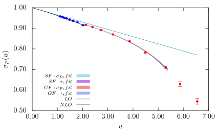
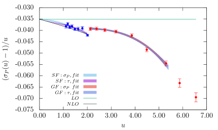
Refer to caption
Figure 3: The plot show the comparison among LO and NLO approximation for the mass anomalous dimension (while the first is valid for any renormalization scheme, the latter is known only in the SF region) and our non perturbative computation. The label $\tau^{SF}$ and $\tau^{GF}$ correspond to two coupling regions.

Having the continuum limit $\sigma(u)=\Sigma_{P}(u,0)$ for various $u$ in both SF and GF regions, to compute the running, we need to obtain an interpolating function for the SSFs. This can be achieved following two (equivalent) strategies: perform a polynomial fit with the ansatz $\sigma_{P}(u)=1+\bar{p}_{0}u+p_{1}u^{2}+p_{2}u^{3}+\mathcal{O}(u^{4})$ with the first coefficient fixed to its perturbative value $\bar{p}_{0}=-d_{0}\log(2)$, or as an alternative approach perform a fit directly for the numerator $\tau(g)$ in (8), viz.

$\displaystyle\sigma_{P}(s,\bar{g}^{2}(\mu))$ $\displaystyle=1+\bar{p}_{0}u+p_{1}u^{2}+p_{2}u^{3}+\mathcal{O}(u^{4})=\exp\left\{-\int_{\sqrt{\bar{g}^{2}(\mu)}}^{\sqrt{\bar{g}^{2}(\mu/s)}}\,\frac{\tau^{\leavevmode\resizebox{8.0pt}{}{NP}}(g^{\prime})}{\beta^{\leavevmode\resizebox{8.0pt}{}{NP}}(g^{\prime})}dg^{\prime}\right\}\,.$ (15)

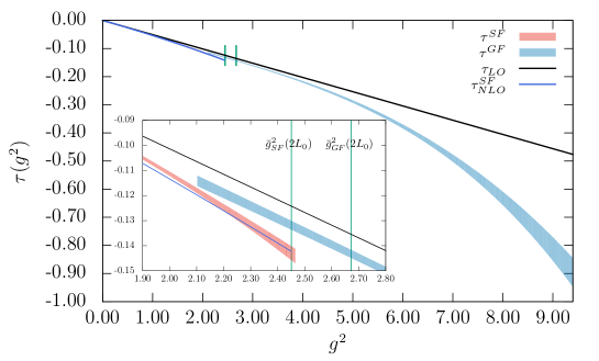
The anomalous dimension, as depicted in Figure 3, is fitted as a polynomial

$\displaystyle\tau^{\leavevmode\resizebox{8.0pt}{}{NP}}(g)$ $\displaystyle=\begin{cases}-g^{2}(\bar{d_{0}}+\bar{d_{1}}g^{2}+d_{2}g^{4}+d_{3}g^{6}+\mathcal{O}(u^{8}))&\text{when $g\in$ SF region}\\ -g^{2}(d_{0}+d_{1}g^{2}+d_{2}g^{4}+d_{3}g^{6}+\mathcal{O}(u^{8}))&\text{when $g\in$ GF region}\end{cases}\;,$ (16)

with coefficients $\bar{d}_{i}$ fixed to their PT values. The fitted expression of $\beta^{\leavevmode\resizebox{8.0pt}{}{NP}}$ in both SF and GF regions [12, 11] is a fundamental input that let us to isolate the anomalous dimension from the ratio in Eq. (8). As displayed in Fig. 1 both approaches discussed above completely agrees within errors. The running from an hadronic scale given by $L_{had}\sim 200\,\rm MeV$ can be written as

$\displaystyle\frac{M}{\bar{m}(L_{had})}$ $\displaystyle=\left.\frac{M}{\bar{m}(L_{pt})}\right|_{SF}\left.\frac{\bar{m}(L_{pt})}{\bar{m}(L_{0})}\right|_{SF}\left.\frac{\bar{m}(L_{0})}{\bar{m}(2L_{0})}\right|_{SF}\left.\frac{\bar{m}(2L_{0})}{\bar{m}(L_{had})}\right|_{GF}\,.$ (17)

The computation of (17) can be split in the following factors: the first term on the rhs is the PT matching, computed at NLO in the SF region with $L_{pt}=L_{0}/2^{N}\sim 65\,\rm GeV$, the second is the standard iterative procedure carried out with the polynomial interpolation of $\sigma_{P}(u)$ for $N=4$ steps (thus gaining a factor $16$ in the scale) given by

$\displaystyle\left.\frac{\bar{m}(L_{pt})}{\bar{m}(L_{0})}\right|_{SF}$ $\displaystyle=\prod_{i=1}^{N}\sigma_{P}(u_{i})\,,$ with $\displaystyle\sigma(u_{i+1})$ $\displaystyle=u_{i}=\bar{g}^{2}(2^{-i}L_{0})\,,$ (18)

the third factor (that could be included in the iteration above) represents the NP scheme matching since it is connecting the two coupling regions

$\displaystyle\left.\frac{\bar{m}(L_{0})}{\bar{m}(2L_{0})}\right|_{SF}$ $\displaystyle=\sigma_{P}(u_{0})\,,$ with $\displaystyle u_{0}$ $\displaystyle=\bar{g}^{2}(L_{0})=2.012\,.$ (19)

The last term is then the ratio of the running from an hadronic scale to the scheme-switching scale. In order to have more flexibility in choosing $L_{had}$ we take advantage of the non-perturbative RG functions and directly determine

$\displaystyle\left.\frac{\bar{m}(2L_{0})}{\bar{m}(L_{had})}\right|_{GF}$ $\displaystyle=\exp\left\{-\int_{\bar{g}(2L_{0})}^{\bar{g}(L_{had})}\frac{\tau_{GF}^{\leavevmode\resizebox{8.0pt}{}{NP}}(g)}{\beta_{GF}^{\leavevmode\resizebox{8.0pt}{}{NP}}(g)}\,dg\right\}\,.$ (20)

Note that here we are computing an integral whose limits are the two scales we want to connect by RG evolution. They do not have to be any more related by an integer scaling factor $s$, as it is being applied in the SSF recursion. In the present work, identifying the hadronic scale with the one corresponding to the most hadronic point222note that this is not the final value defining $L_{had}$ that is covered by the SSF from $u_{GF}=5.3010$, we obtain $L_{had}/L_{0}=18.74(26)$. With this choice, the total range of scales covered by the non-perturbative running in both schemes is $L_{had}/L_{pt}=300(4)$ and finally the total RG running factor $M/\bar{m}(L_{had})=0.9088(78)$.

$u_{\rm SF}$ $L/a$ $\beta$ $\kappa$ $Z_{P}(g_{0}^{2},L/a)$ $Z_{P}(g_{0}^{2},2L/a)$ $\Sigma_{P}(u,a/L)$
6 8.5403 0.13233610 0.80494(22) 0.76879(24) 0.95510(40)
1.1100 8 8.7325 0.13213380 0.79640(22) 0.76163(34) 0.95635(50)
12 8.9950 0.13186210 0.78473(29) 0.75167(59) 0.95786(83)
6 7.2618 0.13393370 0.75460(27) 0.70808(31) 0.93835(53)
1.4808 8 7.4424 0.13367450 0.74425(26) 0.70004(33) 0.94060(55)
12 7.7299 0.13326353 0.73515(33) 0.69193(42) 0.94121(72)
6 6.2735 0.13557130 0.69013(32) 0.62979(37) 0.91256(68)
2.0120 8 6.4680 0.13523620 0.68107(28) 0.62341(43) 0.91535(74)
12 6.72995 0.13475973 0.67113(43) 0.61452(49) 0.91564(93)
16 6.93460 0.13441209 0.66627(31) 0.60924(66) 0.9144(11)
$u_{\rm GF}$ $L/a$ $\beta$ $\kappa$ $Z_{P}(g_{0}^{2},L/a)$ $Z_{P}(g_{0}^{2},2L/a)$ $\Sigma_{P}(u,a/L)$
8 5.3715 0.13362120 0.73275(27) 0.67666(64) 0.9234(9)
2.1257 12 5.5431 0.13331407 0.71301(32) 0.65750(89) 0.9221(13)
16 5.7000 0.13304840 0.70248(32) 0.64369(86) 0.9163(13)
8 4.4576 0.13560675 0.64779(33) 0.56891(75) 0.8782(12)
3.2029 12 4.6347 0.13519986 0.62622(42) 0.54749(94) 0.8743(16)
16 4.8000 0.13482139 0.61735(46) 0.5382(11) 0.8718(19)
8 3.7549 0.13701929 0.52174(47) 0.3924(29) 0.7522(55)
5.3010 12 3.9368 0.13679805 0.50366(53) 0.3652(21) 0.7251(42)
16 4.1000 0.13647301 0.49847(73) 0.3609(23) 0.7240(48)
Table 1: Example of results for $Z_{P}$, $\Sigma_{P}$ in both $\rm SF$ and $\rm GF$ region.

4 Conclusions

We have computed the NP running quark mass in three-flavour QCD between $\sim 200\,\rm MeV$ and $\sim 60\,\rm GeV$ with an unprecedented sub-percent uncertainty. This is a major achievement compared to a similar determinations in the past [7, 13]. In order to optimise the overall precision (in particular towards the hadronic scales), we have employed two different schemes equipped with a non-perturbative at an intermediate scale of $\sim 4\,\rm GeV$. Another completely new results is given by the computation of the NP mass anomalous dimension for both SF and GF coupling regions allowing for a more flexible choice of the hadronic matching scale.

Acknowledgments

The simulations were performed on the Altamira HPC facility, the GALILEO supercomputer at CINECA (INFN agreement), Finisterrae-2 at CESGA and CERN. We thankfully acknowledge the computer resources and technical support provided by the University of Cantabria at IFCA, CESGA, CINECA and CERN. P.F. acknowledges financial support from the Spanish MINECO’s “Centro de Excelencia Severo Ochoa” Programme under grant SEV-2012-0249, as well as from the grant FPA2015-68541-P (MINECO/FEDER).

References

  • [1] M. Papinutto, C. Pena and D. Preti, PoS LATTICE2014 (2014) 281, [1412.1742].
  • [2] M. Lüscher et al., Nucl.Phys. B384 (1992) 168, [hep-lat/9207009].
  • [3] ALPHA, S. Sint and P. Weisz, Nucl.Phys. B545 (1999) 529, [hep-lat/9808013].
  • [4] M. Lüscher et al., Nucl.Phys. B478 (1996) 365, [hep-lat/9605038].
  • [5] ALPHA, S. Capitani et al., Nucl.Phys. B544 (1999) 669, [hep-lat/9810063].
  • [6] ALPHA, G. de Divitiis et al., Nucl.Phys. B437 (1995) 447, [hep-lat/9411017].
  • [7] ALPHA, M. Della Morte et al., Nucl.Phys. B713 (2005) 378, [hep-lat/0411025].
  • [8] ALPHA, P. Fritzsch et al., PoS LATTICE2014 (2014) 291, [1411.7648].
  • [9] P. Fritzsch and A. Ramos, JHEP 1310 (2013) 008, [1301.4388].
  • [10] A. Ramos and S. Sint, Eur. Phys. J. C76 (2016) 15, [1508.05552].
  • [11] ALPHA, M. Dalla Brida et al., (2016), [1607.06423].
  • [12] ALPHA, M. Dalla Brida et al., Phys. Rev. Lett. 117 (2016), [1604.06193].
  • [13] PACS-CS, S. Aoki et al., JHEP 1008 (2010) 101, [1006.1164].