Modulational instability of quantum electron-acoustic waves and associated envelope solitons in a degenerate quantum plasma

Abstract

The basic features of linear and nonlinear quantum electron-acoustic (QEA) waves in a degenerate quantum plasma (containing non-relativistically degenerate electrons, superthermal or $\kappa$-distributed electrons, and stationary ions) are theoretically investigated. The nonlinear Schödinger (NLS) equation is derived by employing the reductive perturbation method. The stationary solitonic solution of the NLS equation are obtained, and examined analytically as well as numerically to identify the basic features of the QEA envelope solitons. It has been found that the effects of the degeneracy and exchange/Bohm potentials of cold electrons, and superthermality of hot electrons significantly modify the basic properties of linear and nonlinear QEA waves. It is observed that the QEA waves are modulationally unstable for $k<k_{c}$, where $k_{c}$ is the maximum (critical) value of the QEA wave number $k$ below which the QEA waves are modulationally unstable), and that for $k<k_{c}$ the solution of the NLS equation gives rise to the bright envelope solitons, which are found to be localized in both spatial ($\xi$) and time ($\tau$) axes. It is also observed that as the spectral index $\kappa$ is increased, the critical value of the wave number (amplitude of the QEA envelope bright solitons) decreases (increases). The implications of our results should be useful in understanding the localized electrostatic perturbation in solid density plasma produced by irradiating metals by intense laser, semiconductor devices, microelectronics, etc.

I Introduction

The signature of electron-acoustic (EA) waves was first observed in the laboratory experiment of Derfler and Simonen DS1969 . This led Watanabe and Taniuti WT1977 to consider a plasma containing electron species of two distinct temperatures and ions, and led to predict theoretically the existence of the EA waves YS1983 in which the restoring force (inertia) is provided by hot electron-temperatre (cold electron mass). The EA wave frequency ($\omega$), in fact, satisfies the condition $\omega_{pi}\ll\omega\leq\omega_{pc}$, where $\omega_{pi}$ ($\omega_{pc}$) is the ion (cold electron) plasma frequency. This means that in the EA waves ions are reasonably assumed to be stationary, and to maintain only the neutralizing background. The dispersion relation for the long-wavelength (in comparision with the hot electron Debye length) EA waves is YS1983 $\omega\simeq kC_{e}$, where $k$ is the wave number, and $C_{e}=(n_{c0}T_{h}/n_{h0}m_{e})^{1/2}$ [where $n_{c0}$ ($n_{h0}$) being the unperturbed cold (hot) electron number density, $T_{h}$ being the hot electron temperature in units of the Boltzmann constant, $m_{e}$ being the cold electron mass] is the electron-acoustic speed. The long wavelength EA waves are also detected in space plasma environments TG1984 ; M-etal2001 ; SL2001 . The conditions for the existence of the linear EA waves and their dispersion properties are now well-understood from both theoretical WT1977 ; YS1983 and experimental DS1969 ; HT1972 points of view. The basic properties of the nonlinear EA waves, particularly EA solitons in electron-ion plasmas have been investigated by several authors MH1990 ; Mace-1991 ; MS2002 ; ref39 .

The nonlinear structures in degenerate plasmas have also received a renewed interest in understanding the localized electrostatic disturbances not only in astrophysical environments (such as neutron stars, white dwarfs, magnetars, etc. Mamun2010a ; Mamun2010b ; El-Taibany2012 ; Hossen2015 ), but also in laboratory devices (viz. solid density plasma produced by irradiating metals by intense laser, semiconductor devices, microelectronics, carbon nanotubes, quantum dots, and quantum wells, etc. Jung2001 ; Ang2003 ; Killian2006 ; Shah2012 ). Recent investigations ref8 ; ref9 ; ref10 ; ref11 based on quantum hydrodynamic (QHD) modelBrodin2007 ; ref12 ; ref13 show a number of significant differences in nonlinear features of quantum plasmas from those in classical electron-ion plasmas. The QHD model is a useful approximation to study the short-scale nonlinear structures in dense (degenerate) quantum plasmas ref12 ; ref13 , where the effects of degenerate (instead of thermal) pressure , exchange correlation potential, and Bohm potential can be included.

Recently, Zhenni et. al. ref45 have studied EA solitary waves or shortly EA solitons in magnetized quantum plasma with relativistic electrons, while Chandra and Ghosh ref46 have studied the modulational instability of the EA waves in relativistically degenerate quantum plasmas. However, they have not considered the exchange correlation and Bohm potentials in their investigation. Therefore, in our present work, we investigate linear and nonlinear propagation of the quantum EA (QEA) waves to include the effects of superthermality ref47 of hot electron component, and quantum effects due to the degenerate particle pressure, exchange correlation and Bohm potentials of cold electron component. We also study the amplitude modulation of the slow evolution of the QEA envelope solitions (QEAESs) by deriving a nonlinear Schrödinger (NLS) equation by taking these effects into account.

The manuscript is organized as follows. The basic equations governing the plasma system under consideration are provided in Sec. II. The NLS equation for the nonlinear propagation of the EA Waves is derived by applying the reductive perturbation technique, and their linear as well as nonlinear properties are examined in Sec. III. A brief discussion is presented in Sec. IV.

II Governing Equations

We consider a three-component plasma system containing cold quantum electron fluid with Fermi energy $E_{F}$ ref12 ; ref13 , inertialess, superthermal MH1990 ; Mace-1991 or hot electron component, and uniformly distributed stationary ions MS2002 . Thus, at equilibrium we have $n_{c0}+n_{h0}=n_{i0}$, where $n_{s0}$ is the number density of plasma species $s$ ($s=c$ for cold electron species, $s=h$ for hot electron species, and $s=i$ for stationary ion species). The dynamics of the QEA waves in such a three-component quantum plasma system is governed by the following set of QHD equations ref12 ; ref13 ; ref4 ; ref48 ; ref51 :

$$\frac{\partial n_{c}}{\partial t}+\frac{\partial}{\partial x}\left(n_{c}v_{c}\right)=0,$$ (1)

$$\frac{\partial v_{c}}{\partial t}+v_{c}\frac{\partial v_{c}}{\partial x}=-\frac{e}{m_{e}}\frac{\partial\phi}{\partial x}-\frac{\partial V_{DB}}{\partial x}-\frac{\partial V_{xc}}{\partial x},$$ (2)

$$\frac{\partial^{2}\phi}{\partial x^{2}}=4\pi e\left(n_{c}+n_{h}-n_{i0}\right),$$ (3)

where $n_{c}$ ($v_{c}$) is the number density (fluid speed) of the cold electron species; $\phi$ is the electrostatic wave potential; $-e$ ($m_{e}$) is the electron charge (mass); $x$ ($t$) is the spatial (time) variable; $V_{DB}=P_{c}/m_{e}n_{c}+V_{B}$, in which $P_{c}$ is the non-relativistically degenerate cold electron pressure, and is given by ref4

$$P_{c}=\frac{\hbar^{2}\pi^{2/3}}{5m_{e}}n_{c}^{5/3},$$ (4)

with $\hbar$ being the Planck constant divided by $2\pi$; $V_{B}$ is the Bohm potential, and is given by ref8 ; ref48

$$V_{B}=\frac{\hbar^{2}}{2m_{e}}\left(\frac{1}{\sqrt{n_{c}}}\frac{\partial^{2}\sqrt{n_{c}}}{\partial x^{2}}\right),$$ (5)

which is due to the tunneling effect of the cold electrons; and $V_{xc}$ is the exchange-correlation potential, and is given by ref48 ; ref51

$$V_{xc}=-0.985e^{2}n_{c}^{1/3}\left[1+\frac{0.624}{a_{B}n_{c}^{1/3}}\ln{\left(1+a_{B}n_{c}^{1/3}\right)}\right],$$ (6)

with $a_{B}=18.37\hbar^{2}/m_{p}e^{2}$. We note that the exchange-correlation potential can be separated into two terms, namely the Hartree term due to the electrostatic potential of the total cold electron number density and the cold electron exchange-correlation potential term ref48 ; ref51 .

The hot electron species is assumed to be superthermal ($\kappa$ distributed). Thus, the number density ($n_{h}$) of the hot electron species is given by MH1990 ; Mace-1991 ; ref47 ; ref39

$$n_{h}=n_{h0}\left[1-\frac{e\phi}{k_{B}T_{h}\left(\kappa-\frac{3}{2}\right)}\right]^{-\kappa+1/2},$$ (7)

where $T_{h}$ is hot electron temperature, and $\kappa$ is the spectral index measuring the deviation from the thermal equilibrium, and its value is $\kappa>3/2$ for superthermal electrons MH1990 ; Mace-1991 ; ref39 .

We now normalize all the variables as follows: $X=x/\lambda_{D}$, $T=t\omega_{pc}$, $V=v_{c}/C_{e}$, $\Phi=e\phi/E_{F}$, $N=n_{c}/n_{c0}$, where $C_{e}=\left(E_{F}/m_{e}\right)^{1/2}$, $\omega_{pc}=(4\pi e^{2}n_{c0}/m_{e})^{1/2}$, $\lambda_{D}=C_{e}/\omega_{pc}$, and $E_{F}=\hbar^{2}(3\pi^{2}n_{c0})^{2/3}/2m_{e}$. Thus, (1)-(3) can be written in the normalized form as

$$\frac{\partial N}{\partial T}+V\frac{\partial N}{\partial X}+N\frac{\partial V}{\partial X}=0,$$ (8)

$$\frac{\partial V}{\partial T}+V\frac{\partial V}{\partial X}=\alpha\frac{\partial\Phi}{\partial X}-\frac{\partial\Psi_{DB}}{\partial X}+\mu N^{-1}\frac{\partial^{3}N}{\partial X^{3}},$$ (9)

$$\frac{\partial^{2}\Phi}{\partial X^{2}}-\delta\Phi-\nu\Phi^{2}=N-1,$$ (10)

where $\Psi_{DB}=3(\sigma N^{2/3}+2\beta N^{1/3})/2$, $\sigma=\hbar^{2}(\pi n_{c0})^{2/3}/m_{e}^{2}C_{e}^{2}$, $\beta=(0.33e^{2}n_{c0}^{1/3}/{m_{e}C_{e}^{2}})[1+0.625/(1+18.37a_{B}n_{pc0}^{1/3})]$, $\mu=(\hbar\omega_{pc}/2m_{e}C_{e}^{2})^{2}$, $\delta=\alpha E_{F}(\kappa+1/2)/k_{B}T_{h}(\kappa-3/2)$, $\nu=\alpha\delta E_{F}(\kappa+1/2)/k_{B}T_{h}(\kappa-3/2)$, and $\alpha=n_{h0}/n_{c0}$.

III Nonlinear Schrödinger Equation

To derive the NLS equation for slow evolution of the QEA waves by the reductive perturbation method Washimi1966 , we first introduce the stretched coordinates:

$$\left.\begin{array}[]{l}\xi=\epsilon(X-v_{0}T),\\ \tau=\epsilon^{2}T,\end{array}\right\}$$ (11)

and expand the dependent variables $N$, $V$, and $\Phi$:

$$N=1+\sum_{n=1}^{\infty}\epsilon^{n}\sum_{l=-\infty}^{\infty}N_{l}^{(n)}(\xi,\tau)\>e^{il(kX-\omega T)},$$ (12)

$$V=\sum_{n=1}^{\infty}\epsilon^{n}\sum_{l=-\infty}^{\infty}V_{l}^{(n)}(\xi,\tau)\>e^{il(kX-\omega T)},$$ (13)

$$\Phi=\sum_{n=1}^{\infty}\epsilon^{n}\sum_{l=-\infty}^{\infty}\Phi_{l}^{(n)}(\xi,\tau)\>e^{il(kX-\omega T)},$$ (14)

where $v_{0}$ is the group velocity of the QEA waves (to be determined later), $\epsilon$ is an expansion parameter ($0<\epsilon<1$), $\omega$ ($k$) is the angular frequency (wave number) of the carrier QEA waves. The quantities $N_{l}^{(n)}(\xi,\tau)$, $V_{l}^{(n)}(\xi,\tau)$, and $\Phi_{l}^{(n)}(\xi,\tau)$ are the $l$-th harmonic of the $n$-th order slowly varying dependent variables, and these satisfy the reality condition $A_{l}^{(n)}\equiv A_{l}^{(n)*}$, in which $*$ denotes the complex conjugate of the quantity involved.

Now, substituting (11)- (14) into (8)-(10), and performing few steps of straight forward mathematics, we can obtain the 1st harmonic of the 1st order ($l=1$ and $n=1$) reduced equations, which allow us to express the linear dispersion for the QEA waves as

$$\omega^{2}=k^{2}\left(\sigma+\beta+k^{2}\mu+\frac{\alpha}{k^{2}+\delta}\right).$$ (15)

We note here that the parameters $\sigma$, $\beta$, and $\mu$ account for the quantum effects due to the degenerate particle pressure, particle exchange-correlation potential, and the Bohm potential, respectively, on the linear dispersion relation for the QEA waves. So, $k^{2}\sigma=T_{DP}$, $k^{2}\beta=T_{XP}$, and $k^{4}\mu=T_{BP}$ represent the quantum effects due to the degenerate particle pressure, particle exchange-correlation potential, and the Bohm potential, respectively. We have shown how these quantum effects (represented by $T_{DP}$, $T_{XP}$, and $T_{BP}$) vary with the carrier QEA wavenumber $k$.

This is displayed in figure 1, where the solid (dotted) curve shows how the effect of electron degenerate pressure (particle exchange potential) varies with $k$, and the dashed curve show how the effect of Bohm potential varies with $k$. It is observed from figure 1 that the effect of the electron degenerate pressure is more significant than that of both exchange-correlation and Bohm potentials. It is further observed from figure 1 that the effect of the exchange-correlation (Bohm) potential is more significant for the smaller (larger) values of the carrier wavenumber $k$. We have graphically shown the effects of superthermality (represented by spectral index $\kappa$) and number density of hot electrons (represented by the parameter $\alpha$) on the dispersion ($\omega$ vs. $k$) curves. These are depicted in figures 2 and 3. They indicate that as $\kappa$ ($\alpha$) increases, the group velocity $v_{0}$ increases for lower (higher) values of $\kappa$ ($\alpha$) , and becomes very sharp at the low value ranges of $\kappa$ and $\alpha$.

It is obvious from figures 2 and 3 that for long wavelength limit (which corresponds to a very low $k$-value range) the angular frequency $\omega$ linearly increases with $k$, and for short wavelength limit (which corresponds to a very high $k$-value range) it is independent of $k$ (saturated region). This is usual dispersion properties of any kind of acoustic-type of waves. It is observed from figure 2 (figure 3) that as we increase $\kappa$ ($\alpha$), the $\omega$ vs. $k$ curve is shifted up (down) to $\omega-$ axis, and the saturation region is reached for higher values of $\kappa$ and $\alpha$.

Now, following the same procedure, from the first harmonic of the second order quantities ($n=2$ and $l=1$), and from (15), we can express $v_{0}$ as

$$v_{0}=\left(\frac{1}{a_{1}\omega+a_{2}k}\right)\left[\omega a_{2}-kb_{1}+2k\left(\omega^{2}-k^{2}b_{0}\right)\right],$$ (16)

where $a_{1}=-k^{2}\alpha/\left(\omega^{2}-k^{2}b_{0}\right)$, $a_{2}=\omega a_{1}/k$, $b_{0}=\sigma+\beta+k^{2}\mu$, and $b_{1}=\alpha+a_{1}b_{0}$. It should be mentioned here that in our present investigation we are interested in the low-frequency, long wavelength QEA waves. We have graphically shown the effects of superthermality (represented by the spectral index $\kappa$) and hot electron number density (represented by the parameter $\alpha$) on $v_{0}$ vs. $k$ curves. The results are depicted in figures 4 and 5.

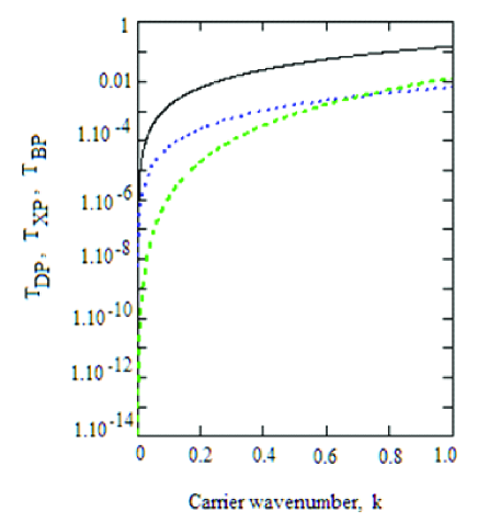
Figure 1: The variation of the quantum terms $T_{DP}$, $T_{XP}$, and $T_{BP}$ with the QEA wavenumber $k$ for $n_{c0}=10^{28}$ cm^-3, $\kappa=1.6$, and $\alpha=0.8$. The solid curve is for $T_{DP}$, the dotted curve is for $T_{XP}$, and the dashed curve is for $T_{BP}$.

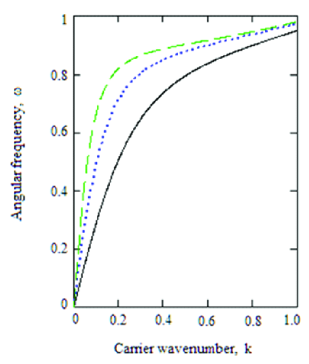
Figure 2: The dispersion ($\omega$ vs. $k$) curves of the QEA waves for $n_{c0}=10^{28}$ cm^-3, $\alpha=0.8$, $\kappa=1.6$ (solid curve), $k=2$ (dotted curve), and $k=50$ (dashed curve).

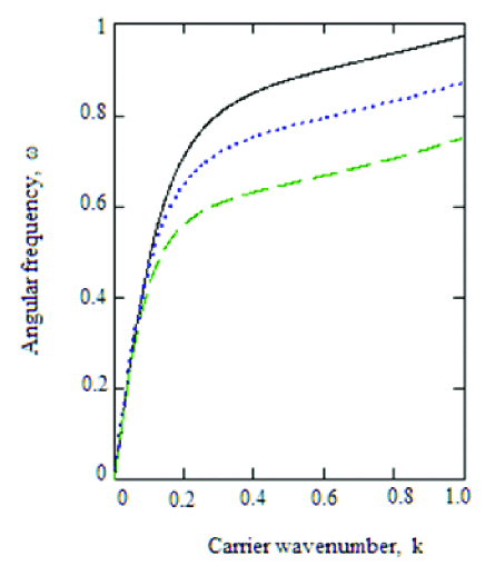
Figure 3: The dispersion ($\omega$ vs. $k$) curves of the QEA waves for $n_{c0}=10^{28}$ cm^-3, $\kappa=2$, $\alpha=0.4$ (solid curve), $\alpha=0.6$ (dotted curve), and $\alpha=0.8$ (dashed curve).

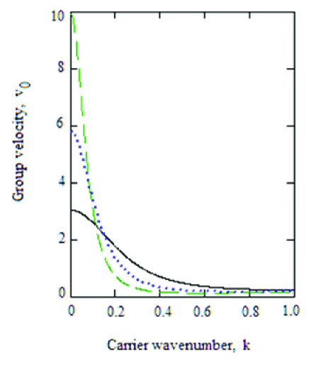
Figure 4: The variation of the QEA wave group velocity $v_{0}$ with the QEA wave number $k$ for $n_{c0}=10^{28}$ cm^-3, $\alpha=0.8$, $\kappa=1.6$ (solid curve), $\kappa=2$ (curve), and $\kappa=50$ (dashed curve).

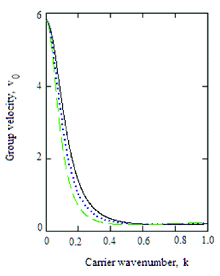
Figure 5: The variation of the QEA wave group velocity $v_{0}$ with the QEA wavenumber $k$ for $n_{c0}=10^{28}$ cm^-3 and $\kappa=2$, $\alpha=0.4$ (solid curve), $\alpha=0.6$ (dotted curve), and $\alpha=0.8$ (dashed curve).

Now, from the 2nd harmonic of the second order ($l=2$ and $n=2$) reduced equations, we can express $\Phi_{2}^{(2)}$ in terms of $\Phi_{1}^{(1)}\Phi_{1}^{(1)}$, which arises from the nonlinear self-interaction. Similarly, from the zeroth harmonic of the third order ($l=0$ and $n=3$) reduced equations, we can express $\Phi_{0}^{(2)}$ in terms of $\left|\Phi_{1}^{(1)}\right|^{2}$. We finally substitute $\Phi_{2}^{(2)}$ and $\Phi_{0}^{(2)}$ into the 1st harmonic $l=1$ of 3rd order ($n=3$) reduced equations to obtain the following NLS equation for the slow evolution of the QEA waves in the form

$$i\frac{\partial a}{\partial\tau}+P\frac{\partial^{2}a}{\partial\xi^{2}}+Q|a|^{2}a=0,$$ (17)

where $a\equiv\Phi_{1}^{(1)}$, and the dispersion and nonlinear coefficients $P$ and $Q$ are

$$P=\left[-\frac{k^{2}\alpha}{a_{1}}+\omega f_{1}+kf_{2}\right]\left[\omega a_{1}+ka_{2}\right]^{-1},$$ (18)

$$Q=\left[\frac{2k^{2}\alpha\nu}{a_{1}}f_{0}+\omega g_{1}+kg_{2}\right]\left[\omega a_{1}+ka_{2}\right]^{-1},$$ (19)

in which $f_{0}$, $f_{1}$, $f_{2}$, $g_{1}$, and $g_{2}$ are listed in the Appendix.

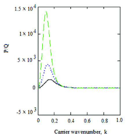
Figure 6: The variation of the ratio $P/Q$ with $k$ for $n_{c0}=10^{28}$ cm^-3, $\alpha=0.8$, $\kappa=1.7$ (sold curve), $\kappa=1.8$ (dotted curve), and $\kappa=2.0$ (dashed curve).

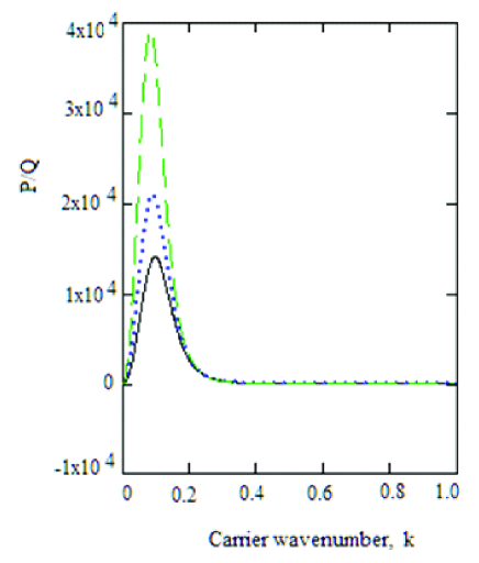
Figure 7: The variation of the ratio $P/Q$ with $k$ for $n_{c0}=10^{28}$ cm^-3, $\kappa=2$, $\alpha=0.4$ (solid curve), $\alpha=0.6$ (dotted curve), and $\alpha=0.8$ (dashed curve).

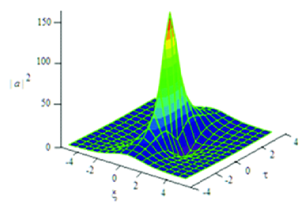
Figure 8: The time dependent envelope solitonic profiles of $|a|^{2}$ for $n_{c0}=10^{28}$ cm^-3, $\alpha=0.6$, and $\kappa=1.8$.

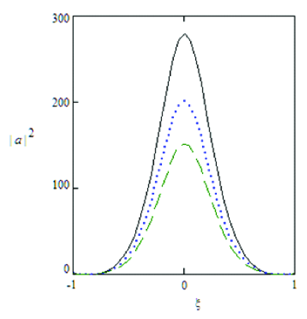
Figure 9: The envelope solitonic profiles of $|a|^{2}$ for $\tau=0$, $n_{c0}=10^{28}$ cm^-3, $\alpha=0.8$, $\kappa=1.6$ (solid curve), $\kappa=1.8$ (dotted curve), and $\kappa=2$ (dashed curve).

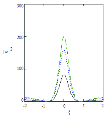
Figure 10: The envelope solitonic profiles of $|a|^{2}$ for $\tau=0$, $n_{c0}=10^{28}$ cm^-3, $\kappa=2$, $\alpha=0.4$ (solid curve), $\alpha=0.6$ (dotted curve), and $\alpha=0.8$ (dashed curve).

The signs of $P/Q$ determine whether the slowly varying wave amplitude is modulationally stable or not. If $P/Q<0$, the wave amplitude is modulationally stable, and the corresponding solution of the NLS equation is called a dark soliton ref56 . On the other hand, if $P/Q>0$, the wave amplitude becomes modulationally unstable, and the solution of the NLS equation in this case is called a bright soliton ref56 . We have graphically shown how $P/Q$ varies with $k$ for different values of $\kappa$ and $\alpha$. These are dipicted in figures 6 and 7. It is observed from figures 6 and 7 that $P/Q$ is positive for lower values of the carrier wavenumber $K$, and it ($P/Q$) changes sign from positive to negative after a certain carrier wavenumber $k=k_{c}$, known as the critical wavenumber. They indicate that the long wavelength QEA waves (i.e. for lower values of $k$, i.e. $k<k_{c}$) are modulationally unstable, and the corresponding solution of the NLS equation gives rise to the bright solitons. On the otherhand, the short wavelength QEA waves (i.e. for higher values of $k$, i.e. $k>k_{c}$) becomes modulationally stable, and the corresponding solution of the NLS equation gives rise to the dark solitons. It is also clear from figures 6 and 7 that the critical wavenumber $k_{c}$ decreases (increases) as we increase the spectral index $\kappa$ ($\alpha$). We are interested in the solution corresponding to the bright solitons (i.e. $P/Q>0$) of the NLS equation, (17), which is given by ref57 ; ref58 :

$$a(\xi,\tau)=a_{0}\left(\sqrt{\frac{P}{Q}}\right)\exp{[iP\tau(\tau)]},$$ (20)

where $a_{0}(x,\tau)=\sqrt{2}[{(4+i16P\tau)}/{(1+16P^{2}\tau^{2}+4\xi^{2})}-1]$. The solution (20) predicts the concentration of the QEA wave in a small region due to the nonlinear properties of the plasma, and it is able to concentrate a significant amount of the wave energy into a relatively small area in space ref57 . We have graphically shown the time dependent bright (envelope) solitons, i. e. the variation of $a*a=|a|^{2}$ with the position ($\xi$) and time ($\tau$). This is displayed in figure 8 which shows how the QEA envelope solitonic profile evolve with time. This surface plot indicates that the QEA waves are localized in both $\xi$ and $\tau$ axes. This feature means that the nonlinear QEA waves can also concentrate the energy of the plasma system in a small region ref59 . The width of the localized structures get flattened along the $\tau$ axis. On the other hand, the stationary envelope solitonic profiles for different values of $\kappa$ and $\alpha$ are shown in figures 9 and 10, respectively. It is obvious from figures 9 and 10 that as we increase the value of $\kappa$ or $\alpha$, the amplitude of the QEA envelope solitons increases, but their width remains unchanged.

IV Discussion

We have considered a three-component degenerate quantum plasma (DQP) system containing cold quantum electron fluid ref12 ; ref13 , inertialess, superthermal MH1990 ; Mace-1991 electrons, and uniformly distributed stationary ions MS2002 to identify the effects of suprathermality ref47 of hot electron component, the degenerate cold electron pressure, cold electron exchange correlation potential, and Bohm potential of cold electron component on the linear and nonlinear properties of the QEA waves. We have derived the NLS equation by the reductive perturbation method, and have obtained its solitonic solution to find the basic features of the QEA envelope solitons. The results, which have been found from this theoretical investigation, can be pinpointed as follows:

1. The quantum effect due to the degenerate electron pressure of the cold electron species dominates over that due to the particle exchange-correlation potential or the Bohm potential on the dispersion properties of the long wavelength QEA waves. However, as the wavelength of the QEA waves is decreased, the effect of the Bohm potential overtakes that of the exchange-correlation potential.

2. It is found that for a long wavelength limit (which corresponds to a very low $k$-value range) the angular frequency $\omega$ linearly increases with $k$, and for a short wavelength limit (which corresponds to a very high $k$-value range) it is independent of $k$ (saturated region). This is usual dispersion properties of any kind of acoustic-type of waves. It is also observed that as we increase $\kappa$ ($\alpha$), the $\omega$ vs. $k$ curve is shifted up (down) to $\omega-$ axis, and the saturation region is reached for higher values of $\kappa$ and $\alpha$.

3. The long wavelength QEA waves (satisfying $k<k_{c}$) are modulationally unstable, and the corresponding solution of the NLS equation gives rise to the bright solitons, where $k_{c}$ is the minimum value of $k$ above which the QEA waves are modulationally stable. On the otherhand, the short wavelength QEA waves (satifying $k>k_{c}$) becomes modulationally stable, the corresponding solution of the NLS equation gives rise to the dark solitons. It is observed that $k_{c}$ is decreased as the spectral index $\kappa$ is increased, and that it is independent of $\alpha$.

4. It is seen that as $\kappa$ ($\alpha$) increases, the group velocity $v_{0}$ increases for lower (higher) values of $\kappa$ ($\alpha$), and becomes very sharp at the low value ranges of $\kappa$ and $\alpha$.

5. It is observed that the QEA waves are localized (as bright envelope solitons) in both $\xi$ and $\tau$ axes, and that as the value of $\kappa$ or $\alpha$ is increased, the amplitude of the QEA envelope solitons increases, but their width remains unchanged. This feature means that the nonlinear waves can concentrate the energy of the plasma system in its small region ref59 .

To conclude, we stress that our present investigation on the QEA waves and associated instability and nonlinear structures in a DQP (containing cold quantum electron fluid ref12 ; ref13 with Fermi energy $E_{F}$, inertialess, superthermal MH1990 ; Mace-1991 electron component. and uniformly distributed stationary ions MS2002 ) is expected to help us to understand the localized low-frequency electrostatic disturbances in laboratory solid density plasma produced by irradiating metals by intense laser, semiconductor devices, microelectronics, carbon nanotubes, etc. Jung2001 ; Ang2003 ; Killian2006 ; Shah2012 . We also suggest to perform a laboratory solid density plasma experiment based on the parameters used in our numerical analysis, which may be able to identify the basic features of linear and nonlinear QEA waves predicted in our present investigation.

Appendix

The notations $f_{0}$, $f_{1}$, $f_{2}$, $g_{1}$, and $g_{2}$ appearing in (18) and (19) are listed as follows:

$$f_{0}=\left[k(X_{2}-\omega a_{1}a_{2})-\nu\Omega\right]X_{1}+\left[2\nu V_{0}-Y_{2}\right]Y_{1},$$

$$f_{1}=v_{0}a_{6}-a_{8},$$

$$f_{2}=v_{0}a_{8}-(\sigma+\beta+3k^{2}\mu)a_{6}+3k\mu a_{1},$$

$$g_{1}=-k[a_{1}(a_{17}+a_{24})+a_{2}(a_{16}+a_{23})],$$

$$g_{2}=k[-a_{2}(a_{17}+a_{24})+a_{1}g_{21}+k^{2}\mu a_{1}g_{22}],$$

where

$$X_{1}=[-k^{2}\alpha+(4k^{2}+\delta)\Omega]^{-1},$$

$$X_{2}=k(X_{\sigma}a_{1}^{2}-a_{2}^{2})/2,$$

$$Y_{1}=[(\sigma+\beta-v_{0}^{2})\delta+\alpha]^{-1},$$

$$Y_{2}=X_{\sigma}a_{1}^{2}+a_{2}^{2}+2v_{0}a_{1}a_{2},$$

$$X_{\sigma}=(\sigma+2\beta)/3+k^{2}\mu,$$

$$\Omega=\omega^{2}-k^{2}b_{1},$$

$$V_{0}=\sigma+\beta-v_{0}^{2},$$

$$g_{21}=(\sigma+2(a_{16}+a_{23})/3,$$

$$g_{22}=7a_{16}+a_{23},$$

$$b_{1}=\sigma+\beta+4k^{2}\mu^{2},$$

$$a_{3}=v_{0}a_{1}-a_{2},$$

$$a_{4}=v_{0}a_{2}+\alpha-a_{1}(\sigma+\beta+3k^{2}\mu^{2}),$$

$$a_{6}=(\omega a_{3}+ka_{4})/(\omega^{2}-k^{2}b_{0}),$$

$$a_{8}=(\omega_{6}-a_{3})/k,$$

$$a_{9}=-2a_{1}a_{2},$$

$$a_{10}=2\beta a_{1}^{2}/3+k^{2}\mu a_{1}^{2},$$

$$a_{11}=-k^{2}\alpha/(\omega^{2}-k^{2}b_{1}),$$

$$a_{12}=(\omega a_{9}-ka_{10})/(\omega^{2}-k^{2}b_{1}),$$

$$a_{13}=\omega a_{11}/k,$$

$$a_{14}=\omega(a_{12}-a_{1}^{2})/k,$$

$$a_{15}=-(a_{12}+\nu/(4k^{2}+\delta+a_{11}),$$

$$a_{16}=a_{11}a_{15}+a_{12},$$

$$a_{17}=a_{13}a_{15}+a_{14},$$

$$a_{18}=2a_{1}a_{2},$$

$$a_{19}=-a_{2}^{2}+(\sigma+2\beta+k^{2}\mu)/3a_{1}^{2},$$

$$a_{20}=\alpha/V_{0},$$

$$a_{21}=(a_{19}-v_{0}a_{18})/V_{0},$$

$$a_{22}=(2\nu-a_{21})/(\delta+a_{20}),$$

$$a_{23}=a_{20}a_{22}+a_{21},$$

$$a_{24}=a_{24}=v_{0}a_{23}-a_{18}.$$

References

- (1) H. Derfler and T. C. Simonen, Phys. Fluids 12, 269 (1969).
- (2) K. Watanabe and T. Taniuti, J. Phys. Soc. Japan 43, 1819 (1977).
- (3) M. Yu and P. K. Shukla, J. Plasma Physics 29, 409 (1983).
- (4) R. L. Tokar and S. P. Gary, Geophys. Res. Lett. 11, 1180 (1984).
- (5) D. S. Montgomery, R. J. Focia, H. A. Rose, D. A. Russell, J. A. Cobble, J. C. Fernańdez, and R. P. Johnson, Phys. Rev. Lett. 87, 155001 (2001).
- (6) S. V. Singh and G. S. Lakhina, Planet. Space Sci. 49, 107 (2001).
- (7) D. Henry and J. P. Treguier, J. Plasma Physics 8, 311 (1972).
- (8) R. L. Mace and M. A. Hellberg, J. Plasma Physics 43, 239 (1990).
- (9) R. L. Mace, S. Baboolal, R. Bharuthram, and M. A. Hellberg, J. Plasma Physics 45, 323 (1991).
- (10) A. A. Mamun and P. K. Shukla, J. Geophys. Res. 107, 1135 (2002).
- (11) S. Sultana and I. Kourakis, Plasma Phys. Control. Fusion 53, 045003 (2011).
- (12) A. A. Mamun and P. K. Shukla, Phys. Plasmas 17, 104504 (2010).
- (13) A. A. Mamun and P. K. Shukla, Phys. Lett. 374, 4238 (2010).
- (14) W. F. El-Taibany and A. A. Mamun, Phys. Rev. E 85, 026406 (2012).
- (15) M. R. Hossen, M. A. Hossen, S. Sultana, and A. A. Mamun, Astrophys Space Sci. 357, 34 (2015).
- (16) Y. D. Jung, Phys. Plasmas 8, 3842 (2001).
- (17) L. K. Ang, T. J. Kwan, and Y. Y. Lau, Phys. Rev. Lett. 91, 208303 (2003).
- (18) T. C. Killian, Nature (London) 441, 297 (2006).
- (19) H. A. Shah, M. J. Iqbal, N. Tsintsadze, W. Masood, and M. N. S. Qureshi, Phys. Plasmas 19, 092304 (2012).
- (20) G. Manfredi and F. Haas, Phys. Rev. B 64, 075316 (2001).
- (21) F. Haas, L. G. Garcia, J. Goedert, and G. Manfredi, Phys. Plasmas 10, 3858 (2003).
- (22) M. Marklund, and P. K. Shukla, Rev. Mod. Phys. 78, 591 (2006).
- (23) M. Akbari-Moghanjoughi, Phys. Plasmas 18, 012701 (2011).
- (24) G. Brodin and M. Marklund, Phys. Plasmas 14, 412607 (2027).
- (25) A. Bret, Phys. Plasmas 14, 084503 (2007).
- (26) F. Hass and A. Bret., Europhys. Lett. 97, 26001 (2012).
- (27) Z. Zhenni, W. Zhengwei, and L. Chunhua, Plasma Sci. Technol. 16, 995 (2014).
- (28) S. Chandra and B. Ghosh, Astrophys. Space Sci. 342, 417 (2012).
- (29) A. Danekha, N. S. Saini, and M. A. Hellberg, Phys. Plasmas 18, 072902 (2011).
- (30) H. Demiray, Phys. Plasmas 23, 032109 (2016).
- (31) P. K. Shukla and B. Eliasson, Rev. Mod. Phys. 83, 885 (2011).
- (32) P. Hohenberg and W. Kohn, Phys. Rev. B 136, 864 (1964).
- (33) H. Washimi and T. Taniuti, Phys. Rev. Lett. 17, 996 (1966).
- (34) A. Hasegawa, Nonlinear Effects and Plasma Instabilities (Springer-Verlag, Berlin, 1975), Chap. 4.
- (35) S. Guo and L. Mei, Phys. Plasmas 21, 112303 (2014).
- (36) W. M. Moslem, R. Sabry, S. K. El-Labany, and P. K. Shukla, Phys. Rev. E84, 066402 (2011).
- (37) N. Akhmediev, A. Ankiewiez, and J. M. Soto-Crespo, Phys. Rev. E 80, 026601 (2009).