Nonlinear reconstruction

Abstract

We present a direct approach to nonparametrically reconstruct the linear density field from an observed nonlinear map. We solve for the unique displacement potential consistent with the nonlinear density and positive definite coordinate transformation using a multigrid algorithm. We show that we recover the linear initial conditions up to the nonlinear scale ($r_{\delta_{r}\delta_{L}}>0.5$ for $k\lesssim 1\ h/\mathrm{Mpc}$) with minimal computational cost. This reconstruction approach generalizes the linear displacement theory to fully nonlinear fields, potentially substantially expanding the baryon acoustic oscillations and redshift space distortions information content of dense large scale structure surveys, including for example SDSS main sample and 21cm intensity mapping initiatives.

I Introduction

The observation of cosmological large scale structure is a cornerstone of modern cosmology. Ambitious surveys are mapping large swaths of the visible Universe (e.g. CHIME Bandura et al. (2014), Tianlai Xu et al. (2015), DESI DESI Collaboration et al. (2016), PFS Takada et al. (2014), and SDSS Alam et al. (2017), etc). Precision measurements of baryon acoustic oscillations (BAO), redshift space distortions (RSD), and primordial non-Gaussianity, etc are continually improving Beutler et al. (2017a); Ross et al. (2017); Vargas-Magaña et al. (2016); Beutler et al. (2017b); Satpathy et al. (2017). The measured BAO scale can constrain the properties of dark energy and the growth rate measured from the RSD effect is crucial for tests of gravity. However, the precision of the measurement is often limited by the strong non-Gaussianities of the dark matter and galaxy density fields on small scales, which prevent a simple mapping to the initial conditions that are predicted by cosmological theories.

The loss of the coherence to the initial conditions has been known as mode-mode coupling, information saturation, etc. Some of the couplings are understood as arising from the coupling of large scale linear modes to smaller scale still linear modes (e.g. cosmic tides Pen et al. (2012); Zhu et al. (2016a); Akitsu et al. (2017), supersample covariance Takada and Hu (2013); Li et al. (2014a, b)). These can be corrected by a linear mapping, also known as “reconstruction” Eisenstein et al. (2007a). The density fluctuations on mildly nonlinear scales can be roughly thought of as the initial linear density fluctuations being translated by the bulk flows. The incoherent bulk flows destroy the coherence to the initial conditions. The density field reconstruction technique reverses the large scale bulk flows using the estimated displacement field Eisenstein et al. (2007a). However, the density field reconstruction methods based on the linear continuity equation only capture the effects of the large scale linear bulk flows instead of the full nonlinear bulk flows.

In this paper, we propose a new approach to reconstruct the linear density field through a nonlinear mapping, which removes most shift nonlinearities. The reconstructed density field given by the displacement potential correlates with the initial linear field to $k\simeq 1\ h/\mathrm{Mpc}$, about a factor of five shorter length scale than observed in Eulerian space. This will substantially improve the measurements of BAO and RSD in the current and future surveys. The new reconstruction scheme offers an incisive tool for probing cosmology and particle physics. We expect the new method to improve cosmological measurement techniques by orders of magnitude to answer many precise questions, e.g. neutrino masses, primordial non-Gaussianities, and modifications to gravity theories.

The paper is organized as follows. Section II presents the reconstruction algorithm. In Sec. III, we apply nonlinear reconstruction to dark matter density field and show reconstruction results. In Sec. IV, we present the physical interpretations for the improved performance. In Sec. V, we discuss future applications of the new reconstruction method.

II Reconstruction algorithm

The basic idea is to build a bijective mapping between the Eulerian coordinate system $\bm{x}$ and a new coordinate system $\bm{\xi}$, where the mass per volume element is constant. We define a coordinate transformation that is pure gradient,

$$x^{i}=\xi^{\mu}\delta^{i}_{\mu}+\frac{\partial\phi}{\partial\xi^{\nu}}\delta^{i\nu},$$ (1)

where $\phi(\bm{\xi})$ is the displacement potential to be solved. The new coordinate system is unique as long as we require the coordinate transformation defined above is positive definite, i.e., $\mathrm{det}(\partial x^{i}/\partial\xi^{\alpha})>0$. We call this new coordinate system potential isobaric gauge/coordinates. It becomes analogous to “synchronous gauge” and “Lagrangian coordinates” before shell crossing, but allows a unique mapping even after shell crossing. Since the Jacobian of Eq. (1) is positive definite, we have $\partial x^{a}/\partial\xi^{a}>0$ (no summation), from which it follows that each Eulerian coordinate is a monotonically increasing function of its corresponding potential isobaric coordinate and vice versa. This implies when we plot the Eulerian positions of the potential isobaric coordinates, the curvilinear grid lines will never overlap.

The unique displacement potential $\phi(\bm{\xi})$ consistent with the nonlinear density and positive definite coordinate transformation can be solved using the moving mesh approach, which is originally introduced for the adaptive particle-mesh $N$-body algorithm and the moving mesh hydrodynamics algorithm Pen (1995, 1998). The moving mesh approach evolves the coordinate system towards a state of constant mass per volume element, $\rho(\bm{\xi})d^{3}\xi=constant$. Since the shift from potential isobaric coordinates to Eulerian coordinates can be large, the displacement potential must then be solved perturbatively. We solve for a coordinate transformation $\Delta\phi^{(i)}$ at each step, where the shift $\nabla\Delta\phi^{(i)}$ is a small quantity, and then calculate the density field in the new coordinate frame. The positive definiteness of the coordinate transformation is achieved through smoothing and grid limiters Pen (1995, 1998). We need to iterate this process for many times until the result converges and obtain the nonlinear bijective mapping from the Eulerian coordinate system to the potential isobaric gauge, $\phi=\Delta\phi^{(1)}+\Delta\phi^{(2)}+\Delta\phi^{(3)}+\cdots$, which results from a continuous sequence of positive definite coordinate transformations. The details of this calculation are given in Appendix A.

We define the negative Laplacian of the reconstructed displacement potential the reconstructed density field,

$$\delta_{r}(\bm{\xi})\equiv-\nabla_{\bm{\xi}}\cdot\nabla_{\bm{\xi}}\phi(\bm{\xi})=-\nabla_{\bm{\xi}}^{2}\phi(\bm{\xi}).$$ (2)

Note that the reconstructed density field is computed in the potential isobaric gauge instead of the Eulerian coordinate system.

III Implementation and results

To test the performance of the reconstruction algorithm, we run a $N$-body simulation with the ${\tt CUBEP^{3}M}$ code Harnois-Déraps et al. (2013). The simulation involves $2048^{3}$ dark matter particles in a box of length $600\ \mathrm{Mpc}/h$ per side. We use the snapshot at $z=0$ and generate the density field on a $512^{3}$ grid. We solve for the displacement potential from the nonlinear density field and then have the reconstructed density field in the potential isobaric gauge. The reconstruction code is mainly based on the CALDEFP and RELAXING subroutines from the moving mesh hydrodynamics code Pen (1998). The details of the numerical implementation are presented in Appendix A.

Figure 1 shows a slice of the nonlinear dark matter density field. We also plot the Eulerian position of each grid point of the potential isobaric gauge. The salient feature is the regularity of the grid. Even in projection, the grid never overlaps itself. This is guaranteed by appropriate smoothing and grid limiters Pen (1998). The distribution of curvilinear grid points becomes denser in the higher density regions and sparser in the lower density regions; as a result the mass per curvilinear grid cell is approximately constant.

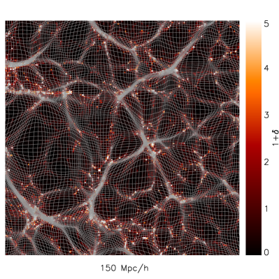
Figure 1: A slice of the nonlinear density field from the simulation. The curvilinear grid shows the Eulerian coordinate of each grid point of the potential isobaric coordinate.

To directly quantify the information of the initial conditions in the density field, we calculate the propagator of the density field,

$$C(\bm{k})=P_{\delta\delta_{L}}(\bm{k})/P_{\delta_{L}}(\bm{k}),$$ (3)

where $\delta_{L}$ is the linear density field scaled to $z=0$ using the linear growth function. The matter power spectrum can be written as

$$P_{\delta}(\bm{k})=C^{2}(\bm{k})P_{\delta_{L}}(\bm{k})+P_{N}(\bm{k}),$$ (4)

where $C^{2}(\bm{k})P_{\delta_{L}}(\bm{k})$ is the linear signal, which is the memory of the initial conditions, and $P_{N}(\bm{k})$ is the power generated in the nonlinear evolution, often referred as the mode-coupling term Crocce and Scoccimarro (2006, 2008); Matsubara (2008). Figure 2 shows the linear signals and the mode-coupling terms for the nonlinear and reconstructed density fields. The linear signal is larger than the mode-coupling term at $k\lesssim 0.6\ h/\mathrm{Mpc}$ after reconstruction, which suggests that all BAO wiggles may be recovered from the present day density field. Even the densest local Universe galaxy surveys such as the SDSS main sample become Poisson noise dominated at this scale, opening up the potential of recovering cosmic information including BAO and potentially redshift-space distortion down to the Poisson noise limit.

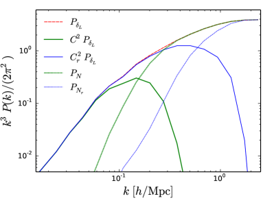
Figure 2: The linear power spectrum (dashed line), the linear signals for the nonlinear (thick solid line) and reconstructed (thin solid line) density fields, and the mode-coupling terms for the nonlinear (thick dotted line) and reconstructed (thin dotted line) density fields. The curves are scaled such that the linear signal plus the mode-coupling term equals the linear power. The linear signal is larger than the mode-coupling term at $k\lesssim 0.6\ h/\mathrm{Mpc}$ after reconstruction.

Reconstruction reduces the nonlinear damping of the linear power spectrum as well as the mode-coupling term. To quantify the overall performance, we compute the cross-correlation coefficients between the density field and the linear initial conditions,

$$r_{\delta\delta_{L}}(\bm{k})=\frac{P_{\delta\delta_{L}}(\bm{k})}{\sqrt{P_{\delta}(\bm{k})P_{\delta_{L}}(\bm{k})}}=\frac{1}{\sqrt{1+\eta(\bm{k})}},$$ (5)

where $\eta(\bm{k})=P_{N}(\bm{k})/(C^{2}(\bm{k})P_{\delta_{L}}(\bm{k}))$ quantifies the relative amplitude of the linear signal to the mode-coupling term. Figure 3 shows the cross-correlation coefficients for the nonlinear and reconstructed density fields. We also plot the cross-correlation coefficient of $\delta_{E}(\bm{q})\equiv-\nabla\cdot\bm{\Psi}(\bm{q})$ with the linear density field, where $\bm{\Psi}(\bm{q})$ is the nonlinear displacement from the simulation. We note that the nonlinear displacement field correlates with the initial density field to even smaller Lagrangian scales. This displacement field is not actually observable, but presumably serves as a hard upper bound on information that could plausibly be recovered from a nonlinear density field, which is scrambled by shell crossing. Several improvements to this reconstruction approach may improve the correlation further, for example using more grid cells or iteratively improving the density field match (see Appendix B). We leave this for future studies, since it would not likely improve the reconstruction from current galaxy surveys. The reconstruction performance on small scales will be limited by the nonlinear galaxy bias and Poisson noise in galaxy surveys.

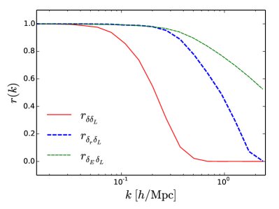
Figure 3: The cross-correlation coefficients with the initial conditions for the nonlinear density field (solid line), the reconstructed density field (thick-dashed line), and the nonlinear displacement (thin-dashed line).

In Fig. 4, we show the joint probability distribution function (PDF) of the reconstructed and linear density fields and the marginal PDFs of the density fields. Since the PDF depends on the grid scale, we apply the Wiener filter $W(\bm{k})=C^{2}_{r}(\bm{k})P_{\delta_{L}}(\bm{k})/P_{\delta_{r}}(\bm{k})$ to both fields to obtain the converged results. The reconstructed densities are well correlated with the initial conditions and the PDF is also apparently much more Gaussian than the nonlinear density field. Therefore, the new reconstruction method is also expected to reduce the correlation between different power spectrum bins and increase the information content Meiksin and White (1999); Scoccimarro et al. (1999); Rimes and Hamilton (2005). Note that all the reconstructed overdensities are smaller than 3 with the maximum value 2.693. The reconstructed density field is given by

$$\delta_{r}(\bm{\xi})=-\nabla_{\bm{\xi}}\cdot(\bm{x}(\bm{\xi})-\bm{\xi})=3-\nabla_{\bm{\xi}}\cdot\bm{x}(\bm{\xi}),$$ (6)

where $\nabla_{\bm{\xi}}\cdot\bm{x}(\bm{\xi})=\sum_{a}\partial x^{a}/\partial\xi^{a}$. The compression limiter constrains $\partial x^{a}/\partial\xi^{a}\geq 0.1$, which implies $\delta_{r}\leq 2.7$ as we indeed observe in the reconstruction. This confirms that the coordinate transformation given by the displacement potential defined in Eq. (1) is positive definite. In the 1D case, the maximum value of the reconstructed density field is smaller than 1 Zhu et al. (2016b), since there is only one spatial dimension in the 1D cosmology McQuinn and White (2016).

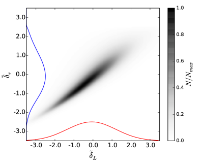
Figure 4: The joint PDF of the reconstructed and linear density field and the marginal PDFs of the density fields. The tilde denotes the field has been Wiener filtered.

IV Physical interpretations

In the Lagrangian picture of structure formation, the Eulerian position $\bm{x}$ of each particle is given by the sum of its Lagrangian position $\bm{q}$ and the subsequent displacement $\bm{\Psi}(\bm{q})$:

$$\bm{x}(\bm{q})=\bm{q}+\bm{\Psi}(\bm{q}).$$ (7)

The density at the Eulerian position $\bm{x}$ is related to the displacement via the mass conservation $\rho(\bm{x})d^{3}x=\bar{\rho}d^{3}q$ or equivalently $[1+\delta(\bm{x})]d^{3}x=d^{3}q$. In the standard reconstruction approach Eisenstein et al. (2007a), the displacement field is given by the linear continuity equation

$$\bm{s}(\bm{k})=\frac{i\bm{k}}{k^{2}}S(k)\delta(\bm{k}),$$ (8)

where $S(k)$ is a Gaussian window function which suppresses the small-scale nonlinearities. The linear mapping defined by the estimated displacement field $\bm{s}({\bm{q}})$ can transform the density field in Eulerian coordinates to the density field in Lagrangian coordinates through the mass conservation. To compute the overdensities at the Eulerian positions $\bm{x}=\bm{q}+\bm{s}(\bm{q})$, instead of assign particles to a curvilinear grid given by $\bm{s}(\bm{q})$, we can displace the particles by the negative displacement $-\bm{s}(\bm{q})$ and then assign particles to a uniform grid to obtain the displaced density field $\delta_{d}(\bm{x})$. To compute the Jacobian of the coordinate transformation, we can shift a set of uniformly distributed particles by the negative displacement $-\bm{s}(\bm{q})$ and calculate the shifted density field $\delta_{s}(\bm{x})$. The Jacobian of the mapping between Lagrangian and Eulerian coordinates is given by $[1+\delta_{s}(\bm{x})]d^{3}x=d^{3}q$. From the mass conservation $[1+\delta_{r}(\bm{q})]d^{3}q=[1+\delta_{d}(\bm{x})]d^{3}x$, we have the reconstructed density field

$$\delta_{r}(\bm{q})=\bigg{[}1+\delta_{d}(\bm{x})\bigg{]}\frac{d^{3}x}{d^{3}q}-1\simeq\delta_{d}(\bm{x})-\delta_{s}(\bm{x}),$$ (9)

where we assume that the shifted density field $\delta_{s}(\bm{x})$ is small such that $[1+\delta_{s}(\bm{x})]^{-1}\simeq 1-\delta_{s}(\bm{x})$. Note that the reconstructed density field $\delta_{r}(\bm{q})$ is not uniform in the estimated Lagrangian coordinates since $\bm{s}(\bm{q})$ is the large-scale linear displacement instead of the full nonlinear displacement $\bm{\Psi}(\bm{q})$. In the new reconstruction approach, we solve the nonlinear mapping between the Eulerian coordinate system and the potential isobaric gauge, where the mass per volume element is constant, and define the negative divergence of the estimated displacement as the reconstructed density field.

In the nonlinear evolution, there are three sources of nonlinearities: bulk flows, shell crossing and structure formation Eisenstein et al. (2007b); Tassev and Zaldarriaga (2012); Tassev (2014). The decay of the propagator for the density field on the mildly nonlinear scales is mainly due to the effects of the bulk motions. The velocity power spectrum peaks at rather large scales, therefore the density fluctuations on mildly nonlinear scales can be crudely thought of as the translated initial density fluctuations, where the translation is given by the displacement field Tassev and Zaldarriaga (2012). The incoherent bulk flows destroy the memory of the initial conditions and cause the decay of the propagator with the characteristic scale given by the root mean square particle displacement. The standard BAO reconstruction approach uses the estimated displacement field from the linear continuity equation to reduce the effects of the large-scale bulk flows (the damping of the linear signal and the mode-coupling term) Padmanabhan et al. (2009); Noh et al. (2009); Seo et al. (2016). However, the new reconstruction scheme captures the full nonlinear displacement to the nonlinear (free-streaming) scale, where shell crossing occurs. The dominant nonlinearities due to the mapping from Lagrangian coordinates to Eulerian coordinates are removed by nonlinear reconstruction except the nonlinearities induced by shell crossing. The nonlinear contribution to the nonlinear displacement field also reduces the correlation between the linear density and nonlinear displacement fields Baldauf et al. (2016); Yu et al. (2017). These nonlinearities arise from nonlinear clustering and therefore can not be removed by the nonlinear mapping from the new reconstruction approach. The potential isobaric gauge avoids most of the shift nonlinearities induced by the coordinate transformation except the inherent nonlinearities due to structure formation (the deviation of $r_{\delta_{E}\delta_{L}}$ from unity) and the residual shift nonlinearities due to shell crossing (the difference between $r_{\delta_{r}\delta_{L}}$ and $r_{\delta_{E}\delta_{L}}$).

V Applications

The reconstructed density field correlates with the initial linear field to the nonlinear scale ($r_{\delta_{r}\delta_{L}}>0.5$ for $k\lesssim 1\ h/\mathrm{Mpc}$) with the linear signal larger than the mode-coupling term for $k\lesssim 0.6\ h/\mathrm{Mpc}$. We expect the reconstructed density field has a comparable fidelity as the linear density field for measuring the BAO scale, since the oscillations in the linear power spectrum are also washed away on small scales. The current BAO reconstruction displaces particles according to the displacement field computed from the observed galaxy density field under some certain model assumptions (the smoothing scale, galaxy bias, and growth rate etc). The reconstruction result depends on the assumed fiducial model and must be tested against different parameter choices. However, we directly solve the displacement potential from the observed density field, which is a purely mathematical problem without any cosmological dynamics involved. The implementation of the new reconstruction algorithm does not need any model assumptions.

There do exist other methods can recover similar correlation with the linear initial conditions, e.g. the Hamiltonian Markov chain Monte Carlo method Wang et al. (2014). However, the Hamiltonian sampling methods can only recover the phase correlation since they have assumed an initial linear power spectrum in the reconstruction. Thus, the Hamiltonian Markov chain Monte Carlo method cannot readily be applied to galaxy surveys to reconstruct the linear BAO signals, since the BAO peak location is already a model input.

The observed galaxy clustering pattern is anisotropic due to the RSD effect. The observed position of a galaxy is shifted from the true position by its peculiar velocity along the line of sight direction, which corresponds to a simple additive offset of the displacement. The reconstructed density field also includes the RSD effect. However, since a lot of nonlinearities are removed by nonlinear reconstruction, both the measurement and modeling of RSD will be improved significantly. We have verified this, however, a detailed study is beyond the scope of this paper and will be presented in the future.

The current velocity reconstruction methods are based on the linear continuity equation. However, we generalize the linear displacement theory to fully nonlinear fields through nonlinear reconstruction. The new velocity reconstruction scheme based on the nonlinear fields is expected to have better performance than the linear theory. Moreover, we expect the new reconstruction method to improve the measurement techniques for the neutrino masses, primordial non-Gaussianities, modifications to gravity theories, etc by orders of magnitude.

Appendix A Reconstruction algorithm

In this Appendix, we present the details of the reconstruction algorithm and its numerical implementation.

In Cartesian coordinates, the continuity equation of fluid dynamics, which epresses the conservation of matter, is

$$\frac{\partial\rho}{\partial t}+\frac{\partial\rho v^{i}}{\partial x^{i}}=0,$$ (10)

where $\rho$ is the fluid density, $\bm{v}$ is the fluid velocity, and $\rho\bm{v}$ is the mass flux density. The total mass of fluid flowing out of a volume element $d^{3}x$ in unit time $\nabla\cdot(\rho\bm{v})d^{3}x$ is the decrease per unit time in the mass of fluid in this volume element $(-\partial\rho/\partial t)d^{3}x$.

We apply a general time-dependent curvilinear coordinate transformation $\bm{x}=\bm{x}(\bm{\xi},t)$ to the continuity equation and obtain

$$\frac{\partial\sqrt{g}\rho}{\partial t}+\frac{\partial}{\partial\xi^{\alpha}}\bigg{[}\sqrt{g}\rho e^{\alpha}_{i}\bigg{(}v^{i}-\dot{x}^{i}\bigg{)}\bigg{]}=0,$$ (11)

where $e^{\alpha}_{i}$ is the matrix inverse of the triad $e^{i}_{\alpha}=\partial x^{i}/\partial\xi^{\alpha}$, and $\sqrt{g}=\mathrm{det}(e^{i}_{\alpha})$ is the volume element. This is the continuity equation in the time-dependent curvilinear coordinate system. However, it also describes the change of the mass per volume element under the time-dependent coordinate transformation $\dot{\bm{x}}$ if the fluid velocity is zero. We can use this equation to evolve the curvilinear coordinate system toward a state of constant mass per volume element across the Universe.

Since we can only observe the density field from galaxy surveys, this allows to determine only the scalar part of the coordinate transformation due to the limited degrees of freedom. We define a coordinate transformation that is a pure gradient $x^{i}=\xi^{\mu}\delta^{i}_{\mu}+({\partial\phi}/{\partial\xi^{\nu}})\delta^{i\nu}$, and set the velocity in Eq. (11) to zero. This results in a linear elliptic evolution equation for the displacement potential $\phi$:

$$\partial_{\mu}(\rho\sqrt{g}e^{\mu}_{i}\delta^{i\nu}\partial_{\nu}\dot{\phi})=\partial_{t}(\sqrt{g}\rho),$$ (12)

where $\dot{\phi}$ is the differential coordinate transformation and $\partial_{t}(\sqrt{g}\rho)$ is the increase per unit time in the mass per unit curvilinear coordinate volume. We use the deviation density $\Sigma=\bar{\rho}-\rho\sqrt{g}$ as the desired change of the mass per volume element,

$$\partial_{\mu}(\rho\sqrt{g}e^{\mu}_{i}\delta^{i\nu}\partial_{\nu}\dot{\phi})=S(\Sigma+C+E),$$ (13)

where $S$ is the smoothing operator, $C$ is the compression limiter, and $E$ is the expansion limiter Pen (1995, 1998). We define the compression limiter $C$ and the expansion limiter $E$ as

$$C(\phi) \equiv 4\bigg{[}\frac{\xi_{m}}{\lambda_{0}}-H\bigg{(}\frac{\xi_{m}}{\lambda_{0}}-1\bigg{)}\bigg{]}^{2},$$ (14)

$$E(\phi,\Sigma) \equiv-2H(\sqrt{g}-v_{m})|\Sigma|,$$ (15)

where $H$ is the Heaviside function, $\xi_{m}\approx 1/10$ is the maximal compression factor, $\lambda_{0}$ is the minimum eigenvalue of the triad $e^{i}_{\mu}$. We choose a typical expansion volume limit $v_{m}=10$. The smoothing operator $S$ is simplest to implement by smoothing over the nearest neighbors in curvilinear coordinates.

We approximate $\bm{x}$ as $\bm{\xi}$ in Eq. (13) and solve for the differential coordinate transformation $\dot{\phi}$ using the multigrid algorithm as described in Ref. Pen (1995). We then calculate the exact change of the mass per volume element $\Delta\rho$ using Eq. (12),

$$\partial_{\mu}(\rho\sqrt{g}e^{\mu}_{i}\delta^{i\nu}\partial_{\nu}\Delta\phi)=\Delta\rho,$$ (16)

where $\Delta\phi=S\dot{\phi}$, and obtain the density field in the new coordinate frame, $\rho^{\prime}=\rho+\Delta\rho$. We iterate this process for many times until the mass per volume element is approximately constant and obtain the displacement potential, $\phi=\Delta\phi^{(1)}+\Delta\phi^{(2)}+\Delta\phi^{(3)}+\cdots$, where $\Delta\phi^{(i)}$ is the solution from the $i$th iteration.

Appendix B Convergence tests

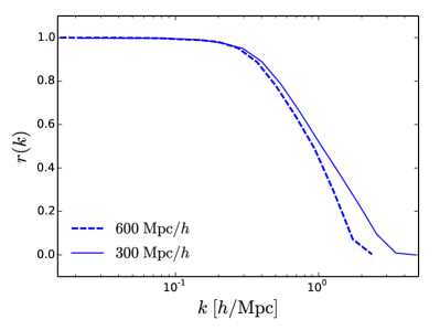
Figure 5: The cross-correlation coefficients between the reconstructed density field and the linear initial conditions for the two simulations with box size $600\ \mathrm{Mpc}/h$ (dashed line) and box size $300\ \mathrm{Mpc}/h$ (solid line).

To check the convergence of reconstruction, we run a simulation with $1024^{3}$ dark matter particles in a box of side length $300\ \mathrm{Mpc}/h$. Due to the sheer computational cost of multigrid calculation with a $1024^{3}$ grid, we instead apply reconstruction to the density field on a $512^{3}$ grid from this small box size simulation. Figure 5 shows the cross-correlation coefficients between the reconstructed density field and the linear initial conditions for the two simulations. We note that using more grid cells can further improve the correlation slightly. However, it would not likely improve the reconstruction from current galaxy surveys because of the nonlinear galaxy bias and Poisson noise on these scales.

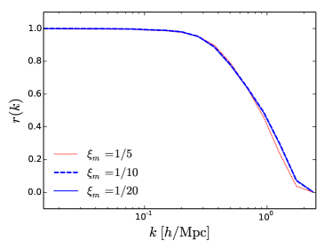
Figure 6: The cross-correlation coefficients between the reconstructed density field and the linear initial conditions for the maximal compression factor $\xi_{m}=(1/5,1/10,1/20)$ and the expansion volume limit $v_{m}=10$.

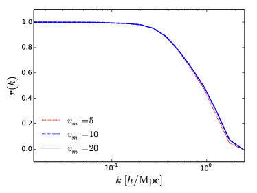
Figure 7: The cross-correlation coefficients between the reconstructed density field and the linear initial conditions for the expansion volume limit $v_{m}=(5,10,20)$ and the maximal compression factor $\xi_{m}=1/10$.

To study how the reconstruction depends on the maximal compression factor $\xi_{m}$ and expansion volume limit $v_{m}$, we perform reconstruction with different $\xi_{m}$ and $v_{m}$. We first set $\xi_{m}=(1/5,1/10,1/20)$ and keep $v_{m}=10$ and apply reconstruction to the nonlinear density field. Figure 6 shows the cross-correlation coefficients of the reconstructed density field with the linear initial conditions for different values of the maximal compression factor. We note that the reconstruction result converges for $\xi_{m}\lesssim 1/10$. To prevent excessive compression and the associated computational cost, we choose $\xi_{m}\approx 1/10$ in the reconstruction. Next we set $v_{m}=(5,10,20)$ and keep $\xi_{m}=1/10$ and apply reconstruction to the nonlinear density field. Figure 7 shows the cross-correlation coefficients of the reconstructed density field with the linear initial conditions for different values of the expansion volume limit. We note that the reconstruction result converges for $v_{m}\gtrsim 10$, so we choose $v_{m}=10$. We expect that $\xi_{m}=1/10$ and $v_{m}=10$ will the optimal choice for most cases of reconstruction in the current galaxy surveys.

References

- Bandura et al. (2014) K. Bandura, G. E. Addison, M. Amiri, J. R. Bond, D. Campbell-Wilson, L. Connor, J.-F. Cliche, G. Davis, M. Deng, N. Denman, et al., in Ground-based and Airborne Telescopes V (2014), vol. 9145 of Proc. SPIE, p. 914522, eprint 1406.2288.
- Xu et al. (2015) Y. Xu, X. Wang, and X. Chen, ApJ 798, 40 (2015), eprint 1410.7794.
- DESI Collaboration et al. (2016) DESI Collaboration, A. Aghamousa, J. Aguilar, S. Ahlen, S. Alam, L. E. Allen, C. Allende Prieto, J. Annis, S. Bailey, C. Balland, et al., ArXiv e-prints (2016), eprint 1611.00036.
- Takada et al. (2014) M. Takada, R. S. Ellis, M. Chiba, J. E. Greene, H. Aihara, N. Arimoto, K. Bundy, J. Cohen, O. Doré, G. Graves, et al., PASJ 66, R1 (2014), eprint 1206.0737.
- Alam et al. (2017) S. Alam, M. Ata, S. Bailey, F. Beutler, D. Bizyaev, J. A. Blazek, A. S. Bolton, J. R. Brownstein, A. Burden, C.-H. Chuang, et al., MNRAS 470, 2617 (2017), eprint 1607.03155.
- Beutler et al. (2017a) F. Beutler, H.-J. Seo, A. J. Ross, P. McDonald, S. Saito, A. S. Bolton, J. R. Brownstein, C.-H. Chuang, A. J. Cuesta, D. J. Eisenstein, et al., MNRAS 464, 3409 (2017a), eprint 1607.03149.
- Ross et al. (2017) A. J. Ross, F. Beutler, C.-H. Chuang, M. Pellejero-Ibanez, H.-J. Seo, M. Vargas-Magaña, A. J. Cuesta, W. J. Percival, A. Burden, A. G. Sánchez, et al., MNRAS 464, 1168 (2017), eprint 1607.03145.
- Vargas-Magaña et al. (2016) M. Vargas-Magaña, S. Ho, A. J. Cuesta, R. O’Connell, A. J. Ross, D. J. Eisenstein, W. J. Percival, J. N. Grieb, A. G. Sánchez, J. L. Tinker, et al., ArXiv e-prints (2016), eprint 1610.03506.
- Beutler et al. (2017b) F. Beutler, H.-J. Seo, S. Saito, C.-H. Chuang, A. J. Cuesta, D. J. Eisenstein, H. Gil-Marín, J. N. Grieb, N. Hand, F.-S. Kitaura, et al., MNRAS 466, 2242 (2017b), eprint 1607.03150.
- Satpathy et al. (2017) S. Satpathy, S. Alam, S. Ho, M. White, N. A. Bahcall, F. Beutler, J. R. Brownstein, C.-H. Chuang, D. J. Eisenstein, J. N. Grieb, et al., MNRAS 469, 1369 (2017), eprint 1607.03148.
- Pen et al. (2012) U.-L. Pen, R. Sheth, J. Harnois-Deraps, X. Chen, and Z. Li, ArXiv e-prints (2012), eprint 1202.5804.
- Zhu et al. (2016a) H.-M. Zhu, U.-L. Pen, Y. Yu, X. Er, and X. Chen, Phys. Rev. D 93, 103504 (2016a), eprint 1511.04680.
- Akitsu et al. (2017) K. Akitsu, M. Takada, and Y. Li, Phys. Rev. D 95, 083522 (2017), eprint 1611.04723.
- Takada and Hu (2013) M. Takada and W. Hu, Phys. Rev. D 87, 123504 (2013), eprint 1302.6994.
- Li et al. (2014a) Y. Li, W. Hu, and M. Takada, Phys. Rev. D 89, 083519 (2014a), eprint 1401.0385.
- Li et al. (2014b) Y. Li, W. Hu, and M. Takada, Phys. Rev. D 90, 103530 (2014b), eprint 1408.1081.
- Eisenstein et al. (2007a) D. J. Eisenstein, H.-J. Seo, E. Sirko, and D. N. Spergel, ApJ 664, 675 (2007a), eprint astro-ph/0604362.
- Pen (1995) U.-L. Pen, ApJS 100, 269 (1995).
- Pen (1998) U.-L. Pen, ApJS 115, 19 (1998), eprint astro-ph/9704258.
- Harnois-Déraps et al. (2013) J. Harnois-Déraps, U.-L. Pen, I. T. Iliev, H. Merz, J. D. Emberson, and V. Desjacques, MNRAS 436, 540 (2013), eprint 1208.5098.
- Crocce and Scoccimarro (2006) M. Crocce and R. Scoccimarro, Phys. Rev. D 73, 063520 (2006), eprint astro-ph/0509419.
- Crocce and Scoccimarro (2008) M. Crocce and R. Scoccimarro, Phys. Rev. D 77, 023533 (2008), eprint 0704.2783.
- Matsubara (2008) T. Matsubara, Phys. Rev. D 77, 063530 (2008), eprint 0711.2521.
- Meiksin and White (1999) A. Meiksin and M. White, MNRAS 308, 1179 (1999), eprint astro-ph/9812129.
- Scoccimarro et al. (1999) R. Scoccimarro, M. Zaldarriaga, and L. Hui, ApJ 527, 1 (1999), eprint astro-ph/9901099.
- Rimes and Hamilton (2005) C. D. Rimes and A. J. S. Hamilton, MNRAS 360, L82 (2005), eprint astro-ph/0502081.
- Zhu et al. (2016b) H.-M. Zhu, U.-L. Pen, and X. Chen, ArXiv e-prints (2016b), eprint 1609.07041.
- McQuinn and White (2016) M. McQuinn and M. White, J. Cosmology Astropart. Phys 1, 043 (2016), eprint 1502.07389.
- Eisenstein et al. (2007b) D. J. Eisenstein, H.-J. Seo, and M. White, ApJ 664, 660 (2007b), eprint astro-ph/0604361.
- Tassev and Zaldarriaga (2012) S. Tassev and M. Zaldarriaga, J. Cosmology Astropart. Phys 4, 013 (2012), eprint 1109.4939.
- Tassev (2014) S. Tassev, J. Cosmology Astropart. Phys 6, 008 (2014), eprint 1311.4884.
- Padmanabhan et al. (2009) N. Padmanabhan, M. White, and J. D. Cohn, Phys. Rev. D 79, 063523 (2009), eprint 0812.2905.
- Noh et al. (2009) Y. Noh, M. White, and N. Padmanabhan, Phys. Rev. D 80, 123501 (2009), eprint 0909.1802.
- Seo et al. (2016) H.-J. Seo, F. Beutler, A. J. Ross, and S. Saito, MNRAS 460, 2453 (2016), eprint 1511.00663.
- Baldauf et al. (2016) T. Baldauf, E. Schaan, and M. Zaldarriaga, J. Cosmology Astropart. Phys 3, 017 (2016), eprint 1505.07098.
- Yu et al. (2017) H.-R. Yu, U.-L. Pen, and H.-M. Zhu, Phys. Rev. D 95, 043501 (2017), eprint 1610.07112.
- Wang et al. (2014) H. Wang, H. J. Mo, X. Yang, Y. P. Jing, and W. P. Lin, ApJ 794, 94 (2014), eprint 1407.3451.