Finite size scaling study of a two parameter percolation model

Abstract

A two parameter percolation model with nucleation and growth of finite clusters is developed taking the initial seed concentration $\rho$ and a growth parameter $\mathtt{g}$ as two tunable parameters. Percolation transition is determined by the final static configuration of spanning clusters. A finite size scaling theory for such transition is developed and numerically verified. The scaling functions are found to depend on both $\mathtt{g}$ and $\rho$. The singularities at the critical growth probability $\mathtt{g}_{c}$ of a given $\rho$ are described by appropriate critical exponents. The values of the critical exponents are found to be same as that of the original percolation at all values of $\rho$ at the respective $\mathtt{g}_{c}$. The model then belongs to the same universality class of percolation for the whole range of $\rho$.

1 Introduction

Percolation is one of the most discussed models of statistical physics of phase transitions that started with the work of Flory in the year 1940 [1] and proposition of a mathematical model by Broadbent and Hammersley in 1957 [2] using the geometrical and probabilistic concepts. Percolation has found extensive applications in different branches of science, such as oil recovery from porous media [3], epidemic modeling [4], networks [5, 6], fracture [7], metal-insulator transition [8], ionic transport in glasses and composites [9], ground water flow in fractured rocks [10] and many others. Percolation refers to the formation of long-range connectedness in a system and is known to be a continuous phase transition from a disconnected to a fully connected phase at a sharply defined percolation threshold value [11, 12]. Beside the uncorrelated ordinary percolation (OP), several correlated percolation models such as bootstrap percolation [13], directed percolation [14], spiral percolation [15], directed spiral percolation [16] are also studied extensively and several non-trivial features were reported. Percolation theory was also applied to study random growth process [17] such as epidemic spreading, rumor propagation, etc. A series of non-equilibrium growth models were proposed in the recent past to demonstrate first order transition that occurs in an explosive manner [18, 19] after the introduction of explosive percolation (EP) by Achlioptas et al [20] in contradiction to second order transition in ordinary percolation. However, most of the EP models are found lacking of several features of first-order transition such as phase co-existence, nucleation, etc. [21, 22].

In this paper, a two parameter percolation model (TPPM) with nucleation and growth of multiple finite clusters simultaneously is proposed taking the initial seed concentration $\rho$ and a growth parameter $\mathtt{g}$ as two tunable parameters. As in OP and unlike growth models, the percolation transition (PT) in this model is determined by the final static or equilibrium spanning cluster configurations. For a given $\rho$, a critical growth probability $\mathtt{g}_{c}$ is found to exist at which a percolation transition occurs. It is then intriguing to characterize the properties as well as the nature of such percolation transitions. It is important to obtain a phase diagram in the $p-\mathtt{g}$ parameter space that separates the disconnected phase from the fully-connected phases.

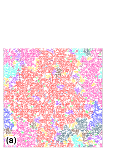
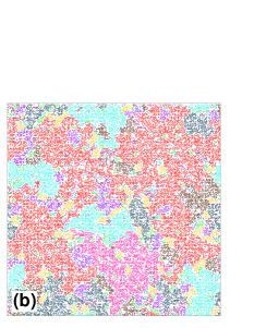
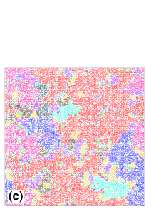
Figure 1: Snapshots of cluster configurations at the end of the growth process on a $2d$ square system of size $L=256$ with initial seed concentration $\rho=0.05$ (a), $0.25$ (b) and $0.50$ (c) at their respective percolation thresholds $\mathtt{g}_{c}(L)=0.560,0.440,0.161$. Solid line represents the lattice boundary. The different colors indicate clusters of different sizes. The spanning clusters are shown in red.

2 Model and simulation

In TPPM, the initial configuration is taken as a partially randomly populated lattice with an initial seed concentration $\rho$ less than $p_{c}$, the threshold of OP and the cluster size distribution is obtained employing Hoshen-Kopelman algorithm [23]. The process of nucleation and growth is then implemented by growing all these finite clusters simultaneously with a constant growth probability $\mathtt{g}$. Note that there are multiple growth centers instead of a single one as in Leath’s OP [24]. Once a site is rejected with probability $(1-\mathtt{g})$, it will remain unoccupied forever, as in ordinary percolation. During the growth of these clusters, two clusters may come in contact. Two clusters with occupied perimeter sites separated by a single lattice spacing are considered to be a single cluster. The total number of clusters is then reduced by one and a cluster of larger size is incorporated in the cluster size distribution. The growth of a cluster stops when there is no empty site on the cluster perimeter is available to occupy. As the process stops, the final cluster size distribution function $n_{s}(\rho,\mathtt{g})$ is obtained. The model has two limiting situations. One is $\rho=p_{c}$, the critical site occupation probability of percolation and $\mathtt{g}=0$. The other one is $\rho=1/L^{2}$, a single seed and $\mathtt{g}=p_{c}$. Both the situations correspond to ordinary percolation problem. The present model can be considered as a generalized multiple cluster growth model of percolation. In the following, taking intermediate values of $\rho$ and varying the growth probability $\mathtt{g}$ transitions from disconnected phase to fully connected phase are studied.

An extensive computer simulation has been performed on two dimensional ($2d$) square lattices of size $L\times L$ varying $L$ from $2^{7}$ to $2^{11}$. For a given $L$, initial seed concentration $\rho$ is varied between $1/L^{2}$ and $0.59$. All finite clusters are identified and grown by occupying the empty nearest neighbours (NN) of the perimeter (both internal and external) sites of these clusters with probability $\mathtt{g}\in[0,1]$. In growing the clusters periodic boundary conditions (PBC) are applied in both the directions. Since the clusters are grown applying PBC, the horizontal and vertical extensions of the largest cluster is kept stored. If either the horizontal or the vertical extension of the largest cluster is found to be $\geq L$, the system size, it is identified as a spanning cluster. The percolation thresholds $\mathtt{g}_{c}$, the probability at which a spanning cluster appears for the first time in the system as $\mathtt{g}$ is increasing to a critical value, are estimated for each $\rho$ on a given $L$. Data are averaged over $10^{5}$ to $10^{6}$ ensembles for each parameter set. Snapshots of the system morphology at the end of the growth process on a square lattice of size $L=256$ with initial seed concentrations $\rho=0.05,0.25$ and $0.50$ are shown in Fig.1 at their respective thresholds $\mathtt{g}_{c}(L)=0.560,0.440,0.161$. In these snapshots, different colors indicate clusters of different sizes. White space corresponds to inaccessible lattice sites. It can be noticed that at the high $\rho$ inaccessible area is less than that at small $\rho$ at their respective thresholds. The spanning cluster is shown in red. Interestingly, irrespective of the values of $\rho$, it seems cluster of all possible sizes appear at their respective percolation thresholds indicating continuous phase transition for all values of $\rho$.

3 Percolation threshold, Critical exponents and Scaling

A scaling theory for TPPM is developed following the techniques of ordinary percolation. In the present model, one starts with an initial seed concentration $\rho$ and the empty sites around the clusters formed by the initial seeds are grown with probability $\mathtt{g}$. The area fraction $p$, number of occupied sites per lattice site, at the end of the growth process is expected to be

$$p=\rho+\mathtt{g}(1-\rho)$$ (1)

if all the remaining empty sites are called for occupation. Since we followed cluster growth process to populate the lattice, it may not always be possible to call all the empty sites except for $\mathtt{g}=1$. As a result, a small area fraction remain inaccessible at the end of the growth process for smaller values of $\rho$. However, for a given $\rho$, the difference in area fractions $p-p_{c}$ corresponding to the growth probability $\mathtt{g}$ and that with $\mathtt{g}_{c}$, the critical threshold, will always be proportional to $(\mathtt{g}-\mathtt{g}_{c})(1-\rho)$ in the critical regime. Hence the scaling form of the cluster size distribution and that of all other related geometrical quantities in TPPM can be obtained in terms of $\mathtt{g}$ and $\rho$ by substituting $p-p_{c}$ by $(\mathtt{g}-\mathtt{g}_{c})(1-\rho)$ in the cluster size distribution of OP as

$$n_{s}(\rho,g)=s^{-\tau}\widetilde{n}_{s}[(\mathtt{g}-\mathtt{g}_{c})(1-\rho)s^{\sigma}]$$ (2)

where $f$ is a new scaling function and $\tau,\sigma$ are new scaling exponents. The scaling form of different geometrical quantities in terms of $\rho$ and $\mathtt{g}$ can be derived from the above cluster size distribution $n_{s}(\rho,\mathtt{g})$ as per their original definitions in terms of $n_{s}(p)$.

3.1 Percolation threshold

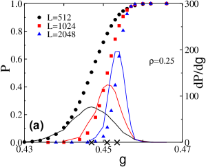
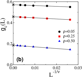
Figure 2: (a) Plot of spanning probability $P$ and its derivative $dP/d\mathtt{g}$ against $\mathtt{g}$ for different system sizes $L$ taking $\rho=0.25$. The symbols are: circle for $L=512$, squares for $L=1024$ and triangles for $L=2048$ and the derivatives are represented by a black line, a red lines and a blue line respectively. The values of $\mathtt{g}$ corresponding to the maxima of the derivatives indicate $\mathtt{g}_{c}(L)$ and marked by crosses. (b) Plot of $\mathtt{g}_{c}(L)$ versus $L^{-1/\nu}$ for $\rho=0.05(\bigcirc),0.25(\square)$ and $0.50(\triangle)$. The best straight line fit is found for $\nu=4/3$. From the intercepts, $\mathtt{g}_{c}(\rho)$ are obtained as $0.5713,0.4570,0.1855$ respectively. (c) Plot of $\mathtt{g}_{c}(\rho)$ against $\rho$. The circles represent the estimated threshold and the line represents the analytic value obtained from Eq.5.

Percolation threshold is identified as the critical growth probability $\mathtt{g}_{c}$ for a given $\rho$ at which for the first time a spanning cluster connecting the opposite sides of the lattice appears in the system. In order to calculate $\mathtt{g}_{c}$ of a given $\rho$ and system size $L$, the probability $P(\rho,\mathtt{g},L)$ to get a spanning cluster is defined as

$$P(\rho,\mathtt{g},L)=\frac{N_{sp}(\rho,\mathtt{g},L)}{N_{tot}}=f[(\mathtt{g}-\mathtt{g}_{c}(\rho))(1-\rho)L^{1/\nu}]$$ (3)

out of $N_{tot}$ ensembles for a system size $L\ll\xi$, the correlation length, $\nu$ is the correlation length exponent. In the limit $L\rightarrow\infty$, $P(\rho,\mathtt{g},L)$ is expected to be a theta function and its derivative with respect to $\mathtt{g}$ would be a delta function at $\mathtt{g}=\mathtt{g}_{c}(\rho)$. Therefore, for a given $\rho$, the value of $\mathtt{g}_{c}(\rho,L)$ at which a spanning cluster appears for the first time is taken as the mean values of the distribution $dP/d\mathtt{g}$ as

$$\mathtt{g}_{c}(\rho,L)=\int_{0}^{1}\mathtt{g}\frac{dP}{d\mathtt{g}}d\mathtt{g}=\mathtt{g}_{c}(\rho)+C\frac{L^{-1/\nu}}{1-\rho},$$ (4)

where $C=\int_{-\infty}^{+\infty}zf^{\prime}(z)dz$, for $z=(\mathtt{g}-\mathtt{g}_{c}(\rho))(1-\rho)L^{1/\nu}$ [25]. In Fig.2(a), for $\rho=0.25$ the probability of having a spanning cluster $P(\rho,\mathtt{g},L)$ is plotted against $\mathtt{g}$ for three different values of $L$. Their derivatives are shown by continuous lines in the same figure in same color of the symbols for a given $L$. The value of $\mathtt{g}_{c}(\rho,L)$ is identified as the value of $\mathtt{g}$ corresponding to the maximum of the derivatives and marked by crosses on the $\mathtt{g}$-axis. In Fig.2(b), $\mathtt{g}_{c}(\rho,L)$ are plotted against $L^{-1/\nu}$ taking $\nu=4/3$ as that of percolation for three different values of $\rho$. It has been verified that the best straight line was found for $\nu=4/3$. The percolation threshold $\mathtt{g}_{c}(\rho)$ for infinite system size is then obtained from the intercepts with the $y$-axis. Since the other geometrical properties are evaluated for selective $\rho$ values, the thresholds $\mathtt{g}_{c}(\rho)$ are also obtained for several values of $\rho$. A phase diagram in the $\rho-\mathtt{g}$ parameter space is constructed by plotting the values of $\mathtt{g}_{c}(\rho)$ against $\rho$ in Fig.2(c). The points constitute a phase line that separates the phase space into percolating and non-percolating regions. It is interesting to note that line connecting the data points satisfies the following equation

$$\rho+\mathtt{g}_{c}(1-\rho)=p_{c}({\rm OP})$$ (5)

where $p_{c}(\approx 0.592746)$ is the percolation threshold of OP. The line of continuous phase transitions terminates at two trivial critical points corresponding to ordinary percolation.

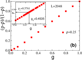
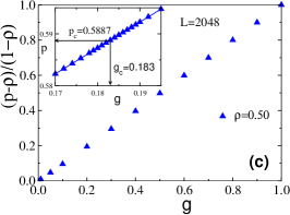
Figure 3: (a) Plot of $(p-\rho)/(1-\rho)$ against $\mathtt{g}$ for $\rho=0.05$(a), $0.25$(b) and $0.50$(c) and for system sizes $L=2048$. In the inset of figures, the area fraction $p$ is plotted against $\mathtt{g}$ within the transition region. The thresholds value of $\mathtt{g}=\mathtt{g}_{c}$ and corresponding $p=p_{c}$ for $L=2048$ is marked by arrow for all $\rho$ values.

Before proceeding further, the critical regime is verified by plotting the variation of $(p-\rho)/(1-\rho)$ against the growth probability $\mathtt{g}$ in Fig.3 for $\rho=0.05$(a), $0.25$(b) and $0.50$(c) and for the system size $L=2048$. It is found to be linear with $\mathtt{g}$ for higher $\rho$ values. Whereas non-linearity arises for smaller values of $\rho$. In the inset, measured $p$ is plotted against $\mathtt{g}$ and found proportional for all values of $\rho$ within the critical region. The thresholds growth probability $\mathtt{g}_{c}$ and the corresponding area fraction $p_{c}$ for $L=2048$ are shown by arrows for all values of $\rho$. The nature of transition at the intermediate values of $\rho$ will be determined now.

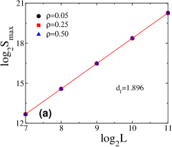
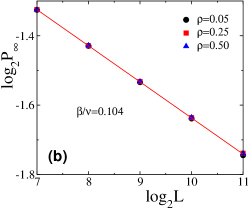
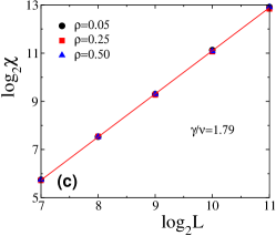
Figure 4: Plot of $S_{max}$, $\chi^{\prime 2}$, $\chi_{\infty}$ and $P_{\infty}$ against system sizes $L$ at their respective thresholds $\mathtt{g}_{c}(\rho)$ for three different values of $\rho=0.05(\bigcirc)$ (black), $0.25(\square)$(red) and $0.50(\triangle)$(blue). The fractal dimension $d_{f}$= 1.896 in (a), $\beta/\nu=0.104$ in (b) and $\gamma/\nu=1.79$ in (c) are estimated from the slope of the straight line and found to be independent of $\rho$.

3.2 Critical exponents

Following the cluster size distribution is given in Eq.2, the order parameter $P_{\infty}$ and the average cluster size $\chi$ can be defined in terms of $\rho$ and $\mathtt{g}$ as

$$P_{\infty}=\frac{S_{max}}{L^{2}}=\rho+\mathtt{g}(1-\rho)-\sideset{}{{}^{\prime}}{\sum}_{s}sn_{s}(\rho,\mathtt{g})$$ (6)

and

$$\chi=\sideset{}{{}^{\prime}}{\sum}_{s}s^{2}n_{s}(\rho,\mathtt{g})$$ (7)

where the primed sum indicates that the spanning cluster is excluded. The percolation spanning cluster is a random object with all possible holes in it and is expected to be fractal. For system size $L$, the size of the spanning cluster $S_{max}$, at the percolation threshold varies with the system size $L$ as

$$\langle S_{max}\rangle\approx L^{d_{f}}$$ (8)

where $d_{f}$ is the fractal dimension of the spanning cluster. Following scaling theory of OP, the scaling behavior of $P_{\infty}$ and $\chi$ are expected to be

$$P_{\infty}\sim[(\mathtt{g}-\mathtt{g}_{c}(\rho))(1-\rho)]^{\beta}\ \ \ {\rm and}\ \ \ \chi\sim[(\mathtt{g}-\mathtt{g}_{c}(\rho))(1-\rho)]^{-\gamma}$$ (9)

where $\beta=(\tau-2)/\sigma$ and $\gamma=(3-\tau)/\sigma$. Presuming that the connectivity (correlation) length $\xi\sim[(\mathtt{g}-\mathtt{g}_{c}(\rho))(1-\rho)]^{-\nu}$, one could also establish that $d_{f}=d-\beta/\nu$. However, the critical exponents measured are very often found to be limited by the finite system size $L$. A system is said to be finite if its size $L$ is less than the connectivity length $\xi$. If a quantity $Q$ is predicted to scale as $|(\mathtt{g}-\mathtt{g}_{c}(\rho))(1-\rho)|^{-q}$ for the system size $L\gg\xi$, then the scaling form of $Q$ for the system size $L\ll\xi$ is expected to be

$$Q(\rho,\mathtt{g},L)=L^{q/\nu}\widetilde{Q}[(\mathtt{g}-\mathtt{g}_{c}(\rho))(1-\rho)L^{1/\nu}]$$ (10)

where $q$ is an exponent $\widetilde{Q}$ is a scaling function. The finite size scaling form of $P_{\infty}$ and the average cluster size $\chi$ are then given by

$$P_{\infty}(\rho,\mathtt{g},L)=L^{-\beta/\nu}\widetilde{P}_{\infty}[(\mathtt{g}-\mathtt{g}_{c}(\rho))(1-\rho)L^{1/\nu}]\ \ \ {\rm and}\ \ \ \chi(\rho,\mathtt{g},L)=L^{\gamma/\nu}\widetilde{\chi}[(\mathtt{g}-\mathtt{g}_{c}(\rho))(1-\rho)L^{1/\nu}].$$ (11)

The values of $S_{max}$, $P_{\infty}$ and $\chi$ are estimated at $\mathtt{g}=\mathtt{g}_{c}(\rho)$ for several systems sizes $L$ as well as for different values of $\rho$. At $\mathtt{g}=\mathtt{g}_{c}(\rho)$, the functions $\widetilde{P}_{\infty}$ and $\widetilde{\chi}$ are expected to be constants. The values of $S_{max}$, $P_{\infty}$ and $\chi$ are plotted against $L$ in double logarithmic scales in Fig.4 (a), (b) and (c) respectively. It can be seen that they follow the respective scaling behaviors. The values of $d_{f}$, $\beta/\nu$ and $\gamma/\nu$ are estimated by linear least square fit through the data points. It is found that $d_{f}=1.896\pm 0.001$, $\beta/\nu=0.104$ and $\gamma/\nu=1.79$. Though the values of critical exponents remain same as previously reported [25], the precise measurements lead to slight modifications in the magnitude of the geometrical quantities. The values of $d_{f}$ and ratios of the exponents as that of OP and hence the phase transition are continuous. It is also important to note that the absolute values of these quantities are independent of the initial seed concentration $\rho$. This means that the area fraction given in terms of $\rho$ and $\mathtt{g}$ in Eq.1 holds correctly at the percolation threshold $\mathtt{g}_{c}(\rho)$ and the spanning clusters of the same size for different $\rho$ are produced. It could also be noted here that in the touch and stop model [26], for low concentration of initial seed the final area fraction was found to be same. The scaling relation $d_{f}=2-\beta/\nu$ is satisfied here within error bars because all critical exponents are as that of percolation.

3.3 Order parameter and its fluctuation

Following the formalism of analyzing thermal critical phenomena [27, 28], the distribution of $P_{\infty}$ is taken as

$$P(P_{\infty})=L^{\beta/\nu}\widetilde{P}[P_{\infty}L^{\beta/\nu}]$$ (12)

where $\widetilde{P}$ is a universal scaling function. Such a distribution function of $P_{\infty}$ is also used in the context of PT recently [21]. With such scaling form of $P_{\infty}$ distribution, one could easily show that $\langle P_{\infty}^{2}\rangle$ as well as $\langle P_{\infty}\rangle^{2}$ scale as $\sim L^{-2\beta/\nu}$. The susceptibility is defined in terms of the fluctuation in $P_{\infty}$ as

$$\chi_{\infty}=\frac{1}{L^{2}}[\langle S_{max}^{2}\rangle-\langle S_{max}\rangle^{2}].$$ (13)

Following the hyper-scaling relation $d\nu=\gamma+2\beta$, the FSS form of $\chi_{\infty}$ is obtained as

$$\chi_{\infty}=L^{\gamma/\nu}\widetilde{\chi}_{\infty}[(\mathtt{g}-\mathtt{g}_{c}(\rho))(1-\rho)L^{1/\nu}]$$ (14)

where $\widetilde{\chi}_{\infty}$ is a scaling function. The finite size scaling form of the order parameter $P_{\infty}(\rho,\mathtt{g},L)$ and its fluctuation $\chi_{\infty}$ are now verified at different values of $\rho$.

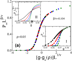
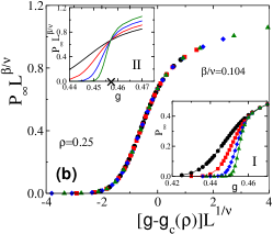
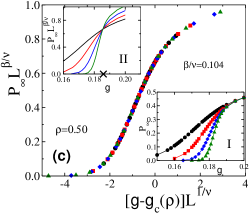
Figure 5: Plot of $P_{\infty}L^{\beta/\nu}$ against $[\mathtt{g}-\mathtt{g}_{c}(\rho)]L^{1/\nu}$ for $\rho=0.05$(a), $0.25$(b) and $0.50$(c) and for $L=256(\bigcirc)$ (black), $512(\square)$ (red), $1024(\Diamond)$ (blue) and $2048(\triangle)$(green). A good data collapse is obtained for the estimated critical exponents $\beta/\nu=0.104$. In inset-I, $P_{\infty}$ $vs$ $\mathtt{g}$ and in inset-II, $P_{\infty}L^{\beta/\nu}$ $vs$ $\mathtt{g}$.

In Fig.5, the variation of $p_{\infty}$ is studied for $\rho=0.05$ (a), $\rho=0.25$ (b) and $\rho=0.50$ (c). In the inset-I of Fig.5, $P_{\infty}$ is plotted against the growth parameter $\mathtt{g}$ for different system sizes $L$ at each $\rho$. Irrespective of the value of $\rho$, the transition become sharper and sharper as $L\rightarrow\infty$ as expected. In the inset-II of Fig.5, the scaled order parameter $P_{\infty}L^{\beta/\nu}$ is plotted against the growth parameter $\mathtt{g}$ for the same system sizes. A precise crossing point at a particular $\mathtt{g}$ is observed for the scaled order parameter of different fixed values of $L$ for a given $\rho$. These crossing points are verified to the critical thresholds $\mathtt{g}_{c}$ of the growth parameter for corresponding values of $\rho$. Finally, the scaled order parameter $P_{\infty}L^{\beta/\nu}$ is plotted against the scaled variable $[\mathtt{g}-\mathtt{g}_{c}(\rho)]L^{1/\nu}$ for different system sizes $L$ at each $\rho$. For each $\rho$, the values of $\beta/\nu$ and $1/\nu$ are taken as that of OP. A good data collapse is observed for all values of $L$ at every value of $\rho$. The distribution of order parameter is found to be a single humped distribution at all values of $\rho$ as in continuous phase transition.

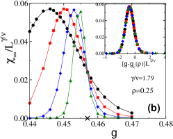
Figure 6: Plot of $\chi_{\infty}/L^{\gamma/\nu}$ against $\mathtt{g}$ for three different $\rho=0.05$ (a), $0.25$ (b) and $0.50$ (c) for the same set of system size as used in FIG. 5. The plots of $\chi_{\infty}/L^{\gamma/\nu}$ for different $L$ are passing through a single point at $\mathtt{g}=\mathtt{g}_{c}(\rho)$ for the particular value of $\gamma/\nu=1.79$. In the inset of figures $\chi_{\infty}/L^{\gamma/\nu}$ are plotted against $[\mathtt{g}-\mathtt{g}_{c}(\rho)]L^{1/\nu}$. A good data collapse is obtained for the estimated critical exponents $\gamma/\nu=1.79$.

The variation in the fluctuation of order parameter $\chi_{\infty}$ is studied as a function of growth parameter $\mathtt{g}$ for the different values of $L$ and $\rho$. In Fig. 6, $\chi_{\infty}/L^{\gamma/\nu}$ are plotted against the growth probability $\mathtt{g}$ for different $L$ at $\rho=0.05$ (a), $\rho=0.25$ (b), $\rho=0.50$ (c) taking $\gamma/\nu=1.79$ as that of OP. The plots intersect a precise value of $\mathtt{g}$ corresponding to $\mathtt{g}$ of respective $\rho$. The maximum values of $\chi_{\infty}/L^{\gamma/\nu}$ remain independent over the system size $L$ at all values of $\rho$ which confirms the value of $\gamma/\nu$ already estimated here. The verification of FSS form of $\chi_{\infty}$ is given in the respective inset of Fig.6 for different values of $\rho$. In the inset, $\chi_{\infty}/L^{\gamma/\nu}$ is plotted against the scale variable $[\mathtt{g}-\mathtt{g}_{c}(\rho)]L^{1/\nu}$, taking the values of $\gamma/\nu$ and $1/\nu$ as that of OP. A good data collapse are found to occur for all values of $\rho$.

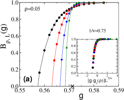
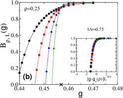
Figure 7: Plot of $B_{\rho,L}(\mathtt{g})$ versus $\mathtt{g}$ for three different $\rho=0.05$ (a), $0.25$ (b) and $0.50$ (c) for the same set of system size as used in FIG. 5. The plot of $B_{\rho,L}(\mathtt{g})$ for different $L$ are passing through a single point at thresholds $\mathtt{g}=\mathtt{g}_{c}(\rho)$, marked by cross on $\mathtt{g}$-axis. In inset, $B_{\rho,L}(\mathtt{g})$ are plotted against $[\mathtt{g}-\mathtt{g}_{c}(\rho)]L^{\beta/\nu}$. A good data collapse is obtained.

3.4 Binder cumulant

The values of the critical exponents and the scaling forms of different geometrical quantities suggest that the PT in TPPM is of continuous second order transition at all values of $\rho$. In order to confirm the nature of transition in TPPM, the $4$th order Binder cumulant (BC) [29],

$$B_{\rho,L}(\mathtt{g})=\frac{3}{2}\left[1-\frac{\langle S_{max}^{4}\rangle}{3\langle S^{2}_{max}\rangle^{2}}\right]$$ (15)

is studied. In Fig.7, $B_{\rho,L}(\mathtt{g})$ is plotted against $\mathtt{g}$ for different $L$ at $\rho=0.05$ (a), $\rho=0.25$ (b) and $\rho=0.50$ (c). For all values of $\rho$, the plots of $B_{\rho,L}(\mathtt{g})$ for different $L$ intersect at a point corresponding to the critical percolation threshold $\mathtt{g}_{c}(\rho)$ of the respective values of $\rho$ as it occurs for a continuous PT. The FSS form of BC is given by,

$$B_{\rho,L}(\mathtt{g})=\widetilde{B}[(\mathtt{g}-\mathtt{g}_{c}(\rho))(1-\rho)L^{1/\nu}],$$ (16)

where $\widetilde{B}$ is a scaling function. The above scaling form is verified in the insets of Fig. 7, plotting BC against $[(\mathtt{g}-\mathtt{g}_{c}(\rho))]L^{1/\nu}$ taking $\nu=4/3$ as that of OP. Good collapse of data are observed at the respective $\mathtt{g}_{c}$ for different values of $\rho$. Thus, for all values of $\rho$ the model represents second order PT that belongs to the same universality class of OP.

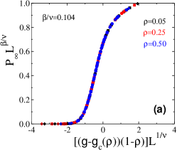
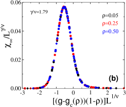
Figure 8: Plot of $P_{\infty}L^{\beta/\nu}$ (a), $\chi_{\infty}/L^{\gamma/\nu}$ (b), $B_{\rho,L}(\mathtt{g})$ (c) and $\chi^{\prime 2}/L^{\gamma/\nu}$ (d) against scaled variable $[(\mathtt{g}-\mathtt{g}_{c}(\rho))(1-\rho)]L^{1/\nu}$ for three different $\rho=0.05$ (black), $0.25$ (red) and $0.50$ (blue) and for three different $L=512(\bigcirc)$, $1024(\square)$ and $2048(\triangle)$. A good data collapse is obtained for all values of $L$ and $\rho$.

3.5 Scaling with $\rho$

Finally, we verify the scaling form of the all the above geometrical quantities as a function of $\rho$, the initial seed concentration. In Fig.8, the respective scaling forms of $P_{\infty}$ (Eq.11), $\chi_{\infty}$ (Eq.14), and $B_{\rho,L}(\mathtt{g})$ (Eq.16) are plotted against the scaled variable $[(\mathtt{g}-\mathtt{g}_{c}(\rho))(1-\rho)]L^{1/\nu}$ for three different values of $\rho$. It can be seen that a very good collapse of data of different $\rho$ occurs for all three geometrical properties [25]. The scaling form presumed for the cluster size distribution in Eq.2 is found to be correct. This is because of the fact that the change in area fraction from its critical value is just proportional to $(\mathtt{g}-\mathtt{g}_{c}(\rho))(1-\rho)$ in the critical regime.

4 Conclusion

A new two parameter percolation model with multiple cluster growth is developed and studied extensively following finite size scaling hypothesis. In this model, two tunable parameters are the initial seed concentration $\rho$ and the cluster growth probability $\mathtt{g}$. It is found that for each $\rho$ there exists a critical growth probability $\mathtt{g}_{c}$ at which a continuous percolation transition occurs. A finite size scaling theory for such percolation transition involving $\rho$ and $\mathtt{g}$ is proposed and verified numerically. It is found that the values of the critical exponents describing the scaling functions at the criticality in this model are that of ordinary percolation for all values of $\rho$. Hence, all such transitions belong to the same universality class of percolation. A phase line consisting of second order phase transition points is found to separate the connected region from the disconnected region in the $\rho-\mathtt{g}$ parameter space. No first order transition is found to occur at any $\rho$ as there is no suppression in the growth of specific clusters.

5 References

References

- [1] P. J. Flory, J. Am. Chem. Soc. 63, 3083, 3091, 3096 (1941).
- [2] S. R. Broadbent and J. M. Hammersley, Percolation processes I. Crystals and mazes, Proc. Camb. Philos. Soc. 53, 629, 641 (1957).
- [3] P. R. King et al., Physica A 274, 60 (1999); Physica A 314, 103 (2002)
- [4] J. L. Cardy and P. Grassberger, J. Phys. A: Math. Gen. 18, L267 (1985).
- [5] R. Cohen, D. Ben-Avraham and S. Havlin, Phys. Rev. E 66, 036113 (2002).
- [6] A. Acin, J. I. Cirac and M. Lewenstein, Nature Physics 3, 256 (2007).
- [7] H. J. Herrmann and S. Roux, editors, Statistical Models for the Fracture of Disordered Media, North-Holland, 1990.
- [8] Z. Ball, H. M. Phillips, D. L. Callahan and R. Sauerbrey, Phys. Rev. Lett. 73, 2099 (1994).
- [9] H. E. Roman, A. Bunde and W. Dieterich, Phys. Rev. B 34, 3439 (1986).
- [10] M. Sahimi, Applications of Percolation Theory, Taylor and Francis, London, 1994.
- [11] D. Stauffer and A. Aharony, Introduction to Percolation Theory, second edition, Taylor and Francis, London, Washington, DC, 1992.
- [12] M. E. J. Newman and R. M. Ziff, Phys. Rev. Lett. 85, 4104 (2000).
- [13] J. Chalupa, P. L. Leath, G. R. Reich, J. Phys. C, Solid State Phys. 12, L31–L35 (1979).
- [14] S. P. Obukhov, Physica A 101, 145 (1980); H. Hinrichsen, Brazilian Journal of Physics 30, 69 (2000).
- [15] S. B. Santra and I. Bose, J. Phys. A 24, 2367 (1991); S. B. Santra and I. Bose, J. Phys. A 25, 1105 (1992).
- [16] S. B. Santra, Eur. Phys. J. B. 33, 75 (2003); S. Sinha and S. B. Santra, Eur. Phys. J. B. 39, 513 (2004).
- [17] A. Aharony, in Fractals and Disordered systems edited by A. Bunde and S. Havlin, Springer-Verlag, Berlin, (1991).
- [18] N. Araújo, P. Grassberger, B. Kahng, K. J. Schrenk, and R. M. Ziff, Eur. Phys. J. Special Topics 223, 2307 (2014) and references therein.
- [19] A. A. Saberi, Phys. Rep. 578, 1 ( 2015 ).
- [20] D. Achlioptas, R. M. D’Souza, and J. Spencer, Science 323, 1453 (2009).
- [21] P. Grassberger, C. Christensen, G. Bizhani, S.-W. Son, and M. Paczuski, Phys. Rev. Lett. 106, 225701 (2011).
- [22] H.-K. Janssen and O Stenull, EPL, 113, 26005 (2016).
- [23] J. Hoshen and R. Kopelman, Phys. Rev. B 14, 8 (1976).
- [24] P.L. Leath, Phys. Rev. B 14, 5046 (1976).
- [25] B. Roy and S. B. Santra, Croat. Chem. Acta. 86, 495 (2013).
- [26] N. Tsakiris, M. Maragakis, K. Kosmidis, and P. Argyrakis, Phys. Rev. E 82, 041108 (2010), Eur. Phys. J.B 81, 303 (2011).
- [27] K. Binder, Z. Phys. B 43, 119 (1981).
- [28] A.D. Bruce, J. Phys. C 14, 3667 (1981).
- [29] K. Binder, Rep. Prog. Phys. 60, 487 (1997).