Level functions of quadratic differentials, signed measures, and the Strebel property

Abstract.

In this paper, motivated by the classical notion of a Strebel quadratic differential on a compact Riemann surface without boundary, we introduce several classes of quadratic differentials (called non-chaotic, gradient, and positive gradient) which possess some properties of Strebel differentials and appear in applications. We discuss the relation between gradient differentials and special signed measures supported on their set of critical trajectories. We provide a characterisation of gradient differentials for which there exists a positive measure in the latter class.

1. Introduction

Theory of quadratic differentials was pioneered in the late 1930’s by O. Teichmüller as a useful tool to study conformal and quasi-conformal maps. Since then it has been substantially extended and found numerous applications. (For the general information about quadratic differentials consult [12, 23, 24].) One important class of quadratic differentials with especially nice properties was introduced by J. A. Jenkins and K. Strebel in the 50’s; these differentials are called Strebel or Jenkins-Strebel, see [5, 12, 24] and § 3 below.

In applications to potential theory, asymptotics of orthogonal polynomials, WKB-methods in spectral theory of Schrödinger equations in the complex domain one often encounters quadratic differentials which are non-Strebel, but rather share some of their properties, see e.g. [1, 4, 14, 15, 20, 22] and references therein. A good example of such non-Strebel differentials having many important properties is provided by polynomial quadratic differentials in $\mathbb{C}$, such that each zero is the endpoint of some critical trajectory.

Motivated by the above examples, we present below several natural classes of differentials containing the class of Strebel differentials and possessing certain nice properties. The most general class we introduce is called non-chaotic and it is characterized by the property that the closure of any horizontal trajectory of such differential is nowhere dense. Further we introduce a natural subclass of non-chaotic differentials which we call gradient and which is characterised by the property that at its smoothness points it is equal to $\pm\Re\sqrt{\Psi}$. Finally, we discuss the appropriate notion of positivity for gradient differentials.

Figure 1. Nikolaĭ Dmitrievich Brashman.

The structure of the paper is as follows. In § 2 we recall the basic facts about quadratic differentials and Strebel differentials. In § 3  we introduce and discuss a number of properties of non-chaotic differentials. In § 4 we introduce and characterize gradient differentials. In § 5 we study positive gradient differentials. Finally, in Appendix I we recall our earlier motivating results relating considered classes of quadratic differentials to the Heine-Stieltjes theory, see [22].

Acknowledgements. The second author wants to acknowledge the hospitality of the Department of Mathematics of UIUC and the financial support of his visits to Urbana-Champaign under the program “INSPIRE” without which this paper would never have seen the light of the day.

2. Crash course on quadratic differentials

2.1. Basic notions

The following definitions are borrowed from [12] and [24].

Definition 1.

A (meromorphic) quadratic differential $\Psi$ on a compact orientable Riemann surface $Y$ without boundary is a (meromorphic) section of the tensor square $(T^{*}_{\mathbb{C}}Y)^{\otimes 2}$ of the holomorphic cotangent bundle $T^{*}_{\mathbb{C}}Y$. The zeros and the poles of $\Psi$ constitute the set of critical points of $\Psi$ denoted by $Cr_{\Psi}$. (Non-critical points of $\Psi$ are called regular.) Zeros and simple poles are called finite critical points while poles of order at least $2$ are called infinite critical points.

The next statement can be found in e.g., Lemma 3.2 of [12].

Lemma 1.

The Euler characteristic of $(T_{\mathbb{C}}^{*}Y)^{\otimes 2}$ equals $2\chi(Y),$ where $\chi(Y)$ is the Euler characteristic of the underlying curve $Y$. Therefore, the difference between the number of poles and zeros (counted with multiplicity) of a meromorphic order $k$ differential $\Psi$ on $Y$ equals $2\chi(Y)$. In particular, the number of poles minus the number of zeros of any quadratic differential $\Psi$ on $\mathbb{CP}^{1}$ equals $4$. Such examples can be found in e.g. [4], Ch. 3.

Obviously, if $\Psi$ is locally represented in two intersecting charts by $f(z)dz^{2}$ and by $\tilde{f}(\tilde{z})d\tilde{z}^{2}$ resp. with a transition function $\tilde{z}(z)$, then $f(z)=\tilde{f}(\tilde{z})\left({d\tilde{z}}/{dz}\right)^{2}.$ Any quadratic differential induces a metric on its Riemann surface $Y$ punctured at the poles of $\Psi$, whose length element in local coordinates is given by

$$|dw|=|f(z)|^{\frac{1}{2}}|dz|.$$

The above canonical metric $|dw|=|f(z)|^{\frac{1}{2}}|dz|$ on $Y$ is closely related to two distinguished line fields spanned by the vectors $\xi\in T_{z}Y$ such that $f(z)dz^{2}$ is either positive or negative. The integral curves of the field given by $f(z)\xi^{2}>0$ are called horizontal trajectories of $\Psi$, while the integral curves of the second field given by $f(z)\xi^{2}<0$ are called vertical trajectories of $\Psi$. Trajectories of $\Psi$ can be naturally parameterised by their arclength. In fact, in a neighbourhood of a regular point $z_{0}$ on $Y,$ one can introduce a local coordinate $w$ called canonicalÊ which is given by

$$w(z):=\int_{z_{0}}^{z}\sqrt{f(\xi)}d\xi.$$

Obviously, in this coordinate the quadratic differential itself is given by $dw^{2}=f(z)dz^{2}$ implying that horizontal trajectories on $Y$ correspond to horizontal straight lines in the $w$-plane.

Since we will only use horizontal trajectories of meromorphic quadratic differentials, we will refer to them simply as trajectories.

Definition 2.

A trajectory of a meromorphic quadratic differential $\Psi$ is called critical, if there exists a finite critical point of $\Psi$ belonging to its closure. For a given meromorphic differential $\Psi$, denote by $K_{\Psi}\subset Y$ the closure of the union of critical trajectories of $\Psi$.

Recall that, by Jenkins’ Basic Structure Theorem [12, Theorem 3.5, pp. 38-39], the set $Y\setminus(K_{\Psi}\cup Cr_{\Psi})$ consists of a finite number of the so-called circle, ring, strip and end domains. (For the detailed definitions and information we refer to loc. cit). The names circle, ring and strip domain are describing their images under the analytic continuation of the mapping given by the canonical coordinate; the end domain (also referred to as half-plane domain)  is mapped by the canonical coordinate onto the half-plane.

The interior of the $K_{\Psi}$ can be non-empty, and consists of a finitely many components, each bounded by a (finite) union of critical trajectories. These components are referred to as the density domains.

The decomposition of $Y\setminus(K_{\Psi}\cup Cr_{\Psi})$ into circle, ring, strip, end and density domains constitutes the so-called domain configuration of $\Psi$.

It is known that quadratic differentials on $\mathbb{CP}^{1}$ with at most three distinct poles do not have density domains, see Theorem 3.6 (three pole theorem) of [12]. This result, in particular, explains Example 1 below in which case the domain configuration consists only of strip and end domains, see e.g. [1]. But starting with 4 distinct poles in $\mathbb{CP}^{1},$ they become unavoidable.

2.2. Strebel differentials

Definition 3.

A compact non-critical trajectory $\gamma$ of a meromorphic $\Psi$ is called closed. It is necessarily diffeomorphic to a circle.

Definition 4.

A quadratic differential $\Psi$ on a compact Riemann surface $Y$ without boundary is called Strebel if the complement to the union of its closed trajectories has vanishing Lebesgue measure.

Remark 1.

In the nomenclature of Definition 2, the complement $Y\setminus(K_{\Psi}\cup Cr_{\Psi})$ for an arbitrary Strebel differential $\Psi$ on $Y$ consists of (finitely many) circular and ring domains, as can be easily deduced from the results of Ch. 3, [24].

One can also easily derive the following statement:

Lemma 2.

If a meromorphic quadratic differential $\Psi$ is Strebel, then it has no poles of order greater than 2. If it has a pole of order 2, then the residue of $\sqrt{\Psi}$ at this pole is negative.

These reasonings are summarized in the next statement.

Lemma 3.

For any Strebel differential $\Psi$ on $Y$, the following holds.

(i) $K_{\Psi}$ is the set of all non-closed horizontal trajectories of $Y$ and $Y\setminus(K_{\Psi}\cup Cr_{\Psi})$ is a disjoint union of finitely many cylinders.

(ii) The metric $|\Psi|$ restricted to any of these cylinders gives the standard metric of a cylinder with some perimeter $p$ given by the length of the horizontal trajectories and some length $l$ given by the length of the vertical trajectories joining the bases of the cylinder. (Notice that $l$ can be infinite.)

(iii) A cylinder is conformally equivalent to the annulus $e^{-l/p}<|z|<1$, or to a punctured disc if $l=\infty$.

Strebel differentials play important role in the theory of univalent functions and the moduli spaces of algebraic curves. They enjoy a large number of extremal properties. Basic results on their existence and uniqueness can be found in Ch. VI of [24], see especially Theorem 21.1.

3. Non-chaotic quadratic differentials

Definition 5.

Given a meromorphic quadratic differential $\Psi$ on a compact Riemann surface $Y$, we say that $\Psi$ is non-chaotic if there exists a continuous and piecewise smooth function

$$F:Y\setminus Cr_{\Psi}\to\mathbb{R}$$

defined on the complement to the set $Cr_{\Psi}$ of critical points of $\Psi$ such that:

(i) $F$ is non-constant on any open subset of $Y\setminus Cr_{\Psi}$,

(ii) yet $F$ is constant on each horizontal trajectory of $\Psi$.

Such a function $F$ is called a level function of $\Psi$.

Example 1.

A polynomial quadratic differential $\Psi=P(z)dz^{2}$, (where $P(z)$ is a univariate polynomial) is non-chaotic on $\mathbb{C}P^{1}$.

It is almost immediate that Strebel differentials are non-chaotic: the distance (in the Riemannian metric induced by $\Psi$) to $K_{\Psi}\cup Cr_{\Psi}$ serves as the level function.

Non-chaotic quadratic differentials are easy to characterise in terms of domain decompositions. Namely, the following statement holds.

Lemma 4.

A quadratic differential $\Psi$ is non-chaotic if and only if $\Psi$ has no density domains, i.e., the closure of each horizontal trajectory of $\Psi$ on $Y$ coincides with this trajectory plus possibly some critical points.

Proof.

Assume non-chaoticity. In this case $K_{\Psi}\cup Cr_{\Psi}$ is a union of finite number of critical trajectories and critical points, and its complement is a union of domains comprised either of compact trajectories (ring and circle domains) or of trajectories isometric to real line (strip and end domains). On each of these domains we can construct a function that is continuous, constant on the trajectories, but not on any open set, and which is vanishing on the boundary of the domain (e.g. by taking the sine of the imaginary part of the canonical coordinate). Gluing together these functions (originally defined on individual domains, but vanishing on the boundary) along $K_{\Psi}$ delivers the desired continuous level function.

If $\Psi$ is chaotic, there exists a trajectory with closure having a non-empty interior. A level function should be constant on this trajectory and continuous, hence constant on an open set, a contradiction. ∎

As we mentioned, any Strebel differential is non-chaotic. Moreover, the following holds.

Proposition 1.

A quadratic differential $\Psi$ is Strebel if and only if it is non-chaotic and has a level function $F$ with finite limits at each critical point $p\in Cr_{\Psi}$, i.e. a level function $F$ that can be extended by continuity from $Y\setminus Cr_{\Psi}$ to $Y$.

Proof.

As we mentioned above, a non-chaotic differential is Strebel if and only if its domain decomposition consists only of ring and circle domains. It is clear that in this case the construction of Lemma 4 yields a function continuous on all of $Y$. Conversely, the existence of an end or a strip domain implies that there is a one-parametric family of non-critical trajectories converging (on one end of the strip) to a critical point $C_{o}\in Cr_{\Psi}$. The union of these trajectories forms a sub-strip in a strip or an end domain. A non-constant function on such a sub-strip which is constant along the trajectories will automatically have discontinuity at $C_{o}$. ∎

To move further, let us recall some basic facts from complex analysis and potential theory on Riemann surfaces, see e.g. [7].

Let $Y$ be an (open or closed) Riemann surface and $h$ be a real- or complex-valued smooth function on $Y$.

Definition 6.

The Levy form of $h$ (with respect to a local coordinate $z$) is given by

$$\mu_{h}:=2i\frac{\partial^{2}h}{\partial z\partial\bar{z}}\;dz\wedge d\bar{z}.$$ (3.1)

In terms of the real and imaginary parts $(x,y)$ of $z,$ $\mu_{h}$ is given by

$$\mu_{h}=\left(\frac{{\partial}^{2}h}{{\partial}x^{2}}+\frac{{\partial}^{2}h}{{\partial}y^{2}}\right)\;dx\wedge dy=\Delta hdx\wedge dy.$$

If $h$ is a smooth real-valued function, $\mu_{h}$ can be also thought of as a real signed measure on $Y$ with a smooth density. In potential theory $h$ is usually referred to as the (logarithmic) potential of the measure $\mu_{h}$, see e.g. [7], Ch.3. Notice that (3.1) makes sense for an arbitrary complex-valued distribution $h$ on $Y$ if one interprets $\mu_{h}$ as a 2-current on $Y$, i.e. a linear functional on the space of smooth compactly supported functions on $Y$, see e.g. [3].

Such a current is necessarily exact since the inclusion of smooth forms into currents induces the (co)homology isomorphism. Recall that any complex-valued measure on $Y$ is a $2$-current characterised by the additional requirement that its value on a smooth compactly supported function depends only on the values of this function, i.e. on its $0$-jet (and does not depend on its derivatives, i.e. on higher jets). Notice that if $Y$ is compact and connected, then exactness of $\mu_{h}$ is equivalent to the vanishing of the integral of $\mu_{h}$ over $Y$.

We should remark here that the Levy form depends on the (local) metric structure defined by the (local) coordinate $z$, unless it is a sum of the delta-functions.

Example 2.

a) If $h=\ln|z|$ on ${{\mathbb{C}}{\rm P}}^{1}$, then $\mu_{h}$ is a real measure supported on the $2$-point set $\{0,\infty\}$ with $\mu_{h}(0)=2\pi$, $\mu_{h}(\infty)=-2\pi$.

b) If $h=|\Im z|$ on $\mathbb{C}$, then $\mu_{h}$ is a measure supported on the real axis, namely, $\mu_{h}=2dx$, i.e. twice the usual Lebesgue measure on the real line.

The easiest way to verify these examples is to use Green’s formula:

$$\mu_{h}(D)=\int_{D}2i\;{\partial}{\bar{\partial}}h=\int_{{\partial}D}\frac{{\partial}h}{{\partial}n}dl,$$

which provides a way to calculate $\mu_{h}(D)$ where $D$ is a arbitrary compact domain in $Y$ with a smooth boundary; $\frac{{\partial}h}{{\partial}n}$ is the derivative of $h$ w.r.t the outer normal, and $dl$ is the length element of the boundary.

$$\int_{D}f\Delta h=-\int_{D}(df,dh)+\int_{{\partial}D}f\frac{{\partial}h}{{\partial}n}dl.$$

Here $D$ is a domain bounded by a piecewise smooth loop ${\partial}D$ orinted counterclockwise; ${\partial}h/{\partial}n$ is the derivative in the orthogonal direction to ${\partial}D$, while $dl$ is the length element on ${\partial}D$.

Our next goal is, for a given non-chaotic $\Psi$, to find its level function $F$ which is closely related to the metrics on $Y$ induces by $\Psi$ or, alternatively, whose Levi form $\mu_{F}$ has a small support. Such $F$ is readily available by the following statement.

Proposition 2.

For any non-chaotic differential $\Psi$ on $Y$, there exist its level functions which are piecewise harmonic and which are non-smooth on finitely many trajectories of $\Psi$.

Proof.

Take as $F$ the distance to $K_{\Psi}\cup Cr_{\Psi}$ in the metric defined by $\Psi$. Locally, its differential coincides with $\Im\sqrt{\Psi}$, hence is harmonic. It is immediate that $F$ is smooth outside $K_{\Psi}\cup Cr_{\Psi}$ and the (finite) union of the horizontal trajectories running in the middle of the strip and annular domains. ∎

Remark 2.

We will call level functions constructed in Proposition 2 piecewise harmonic. For any piecewise harmonic level function $F$, its Levy form $\mu_{F}$ is a well-defined $2$-current supported on the union of $Cr_{\Psi}$ and finitely many trajectories where $F$ is non-smooth. For example, in case of a Strebel differential $\Psi$, the Levy form of any piecewise harmonic level function will have point masses exactly at the double poles of $\Psi$.

4. Gradient differentials

Denote by $\bar{K}_{\Psi}$ the union of the critical trajectories and the zeros and simple poles of $\Psi$,

$$\bar{K}_{\Psi}=K_{\Psi}\cup Cr^{\mathtt{f}}\Psi.$$

This is a one-dimensional cell complex embedded into $Y\setminus Cr^{-}_{\Psi}$, where $Cr^{-}_{\Psi}$ is the union of all infinite critical points and equipped with a metric (given by $|d\Im\sqrt{\Psi}|$) that turns $\bar{K}_{\Psi}$ into a complete metric space (the topologically open ends of the graph have an infinite length).

Consider the decomposition

$$\bar{K}_{\Psi}=\amalg_{\alpha\in A}\bar{K}_{\alpha}$$

into the set of its connected components.

Each of these components also carries the structure of the fat graph, encoded by the collection of cyclic permutations of the edges incident to a given vertex, one for each vertex of the graph.

These cyclic permutations can be thought of as a single permutation $\sigma_{0}$ of the set of flags of a graph, that is of the pairs consisting of a vertex and its incident edge; the orbits of the permutation $\sigma_{0}$ are in one-to-one correspondence with the vertices of the fat graph.

The other permutation of the flags of the fat graph is the involution $\sigma_{1}$ interchanging the two flags corresponding to the same edge.

The composition cycles of the product $\sigma_{0}\sigma_{1}$ correspond to the boundary components of the fat graph, which list the trajectories bounding the connected components of the complement $Y\setminus K_{\Psi}$ in the order fixed by the orientation.

We define the Reeb graph $\mathit{Rg}_{\Psi}$ of a non-chaotic quadratic differential $\Psi$ as follows.

Definition 1.

The Reeb graph $\mathit{Rg}_{\Psi}$ is the metric graph with possibly edges of infinite length necessarily ending at leaves. The vertices $V_{\Psi}=A$ of the Reeb graph are identified with the set of connected components of $\bar{K}_{\Psi}$. The edges $E_{\Psi}$ are the spaces of noncritical trajectories (or, equivalently, the factor spaces of the connected components of $Y\setminus K_{\Psi}$ by the equivalence relations given by belonging to the same trajectory). The lengths on the edges are given by $|\int\Im\sqrt{\Psi}|$.

The Reeb graph $\mathit{Rg}_{\Psi}$ might have loops and multiple edges. We remark that on each of the connected components of $Y\setminus K_{\psi}$, the square root of the quadratic differential is the meromorphic 1-form $\sqrt{\Psi}$ defined unambiguously, up to a sign.

The lengths of the edges are finite for the strip or ring components, and infinite for the circle or end components. The components corresponding to edges of infinite length are necessarily adjacent to the poles of order at least $2$, i.e. to the infinite critical points.

We will call a level function $F$ natural if on any of the connected components of $Y\setminus K_{\Psi}$, its gradient matches the real part of a branch of $\sqrt{\Psi}$:

$$dF=\pm\Re\sqrt{\Psi}.$$

A natural level function fixes the orientation on each of the edges of the Reeb graph $\mathit{Rg}_{\Psi}$. Together with the length elements on the edges, these orientations define a family of 1-forms on the edges, and hence a de Rham cocycle on the Reeb graph $\mathit{Rg}_{\Psi}$.

Proposition 3.

A non-chaotic differential $\Psi$ admits a natural level function if and only if the edges of $\mathit{Rg}_{\Psi}$ can be oriented in such a way that the resulting $1$-cocycle on $\mathit{Rg}_{\Psi}$ is trivial. In other words, the sum of the lengths of the edges in any oriented cycle in the Reeb graph, taken with the signs $\pm$ depending on whether the orientation of the cycle is consistent with the orientations of the edges or not, vanishes.

Conversely, any such orientation defines a natural level function up to an additive constant.

Definition 7.

Any non-chaotic quadratic differential satisfying the conditions of Proposition 3 will be called gradient, and any of the corresponding level functions $F$ will be called a potential.

Any potential of a gradient quadratic differential is constant on the components of $\bar{K}_{\Psi}$.

Proof of Proposition 3.

The claim that a potential defines an orientation on the edges of the Reeb graph is immediate from the definition, as is the exactness of that cocycle. Conversely, the exactness of the cocycle on the Reeb graph defined by the length elements and orientations on the edges allows one to integrate it to a function on the Reeb graph, which lifts to a potential. ∎

Lemma 5.

Levy form $\mu_{F}$ of any potential $F$ of a gradient quadratic differential $\Psi$ is supported on $K_{\Psi}\cup Cr_{\Psi}$.

Proof.

Indeed, the restriction of the potential to each of the domains in $Y\setminus(K_{\Psi}\cup Cr_{\Psi})$ is harmonic. ∎

The potential functions may fail to exist (for example, if the Reeb graph has a loop). But their number is obviously finite (as we can identify the potential functions with an element of the finite set of orientations of the edges of the Reeb graph). In fact, more can be said:

Proposition 4.

For a gradient differential $\Psi$, the number of different potentials (considered up to an additive constant) is either $0$ or a power of 2, comp. Theorem 4 of [22].

Proof.

The group $\mathtt{Flips}=\mathbb{Z}_{2}^{E_{\Psi}}$ of flipping the orientations of the edges acts on the space of cochains on the Reeb graph by reflections. The collections of flips that preserve the subspace annihilating the cycles in the Reeb graph is, clearly, a subgroup in $\mathtt{Flips}$. ∎

Existence of the potential function poses further restrictions on the local properties of the quadratic differential $\Psi$.

Let $F$ be a potential for $\Psi$. We will refer to a pole of $\Psi$ as $F$-clean if it does not belong to the support of the Levy measure $\mu_{F}$.

Lemma 6.

The order $r\geq 2$ of any $F$-clean pole is even.

Proof.

Indeed, the $\mathbb{Z}_{2}$-bundle of orientations defined by $\pm dF$ does not admit a section in a (punctured) vicinity of a pole of $\Psi$ of odd order. Hence $dF$ is discontinuous in an arbitrarily small neighbourhood of the pole. ∎

The $F$-clean poles of even order exist. Moreover,

Proposition 5.

Let $F$ be a potential for a non-chaotic quadratic differential $\Psi$. Then for any $F$-clean pole $z_{*}$ of $\Psi$ of even order, the residue of the $\sqrt{\Psi}$ (defined up to a sign near $z_{*}$) is purely imaginary.

Proof.

The statement follows immediately from the fact that for a clean pole, $F$ is smooth in a punctured vicinity of $z_{*}$, and therefore the increment of the potential $F$ equals the residue of $\sqrt{\Psi}$. ∎

Lemma 7.

A gradient differential $\Psi$ on a compact $Y$ is uniquely defined by its Levy form $\mu_{F}$ of any of its potentials $F.$

Proof.

Two functions $F_{1}$ and $F_{2}$ (considered as 0-currents) have the same Levy forms (considered as 2-currents) only if the difference $F_{1}-F_{2}$ has vanishing Laplacian, and hence, by compactness of $Y$, is a constant.

Now, if two gradient quadratic differentials $\Psi_{1},\Psi_{2}$ have corresponding potentials $F_{1},F_{2}$ coinciding (up to a constant) on an open subset of $Y$, then the (locally defined) holomorphic 1-forms $\sqrt{\Psi}_{1},\sqrt{\Psi}_{2}$ have identical real parts (equal to $dF_{1},dF_{2}$, respectively) on the same subset, and hence coincide everywhere.

∎

5. Levy measures and Positivity

In this section we discuss the notion of positivity for gradient quadratic differentials. Observe that for any potential function $F$, its Levy form $\mu_{F}$ is an exact $2$-current on $Y$, i.e., $\int_{Y}\mu_{F}=0$. Many applications in asymptotic analysis lead to the situation when a gradient differential has a potential $F$ whose Levy form is a signed measure whose positive part is supported on $K_{\Psi}$, and whose negative part is supported on ($F$-clean) poles of $\Psi$. (We discuss an example in § 6.)

Definition 8.

We will call positive a clean potential $F$ such that the restriction of $\mu_{F}$ to $K_{\Psi}$ is a positive measure. A quadratic potential admitting a positive potential will also be referred to as positive.

We remark that the notion of positivity depends only on the potential function $F$ but not on the particular coordinate chart.

Whether or not a potential of a gradient quadratic differential $\Psi$ is positive, depends not only on its Reeb graph, but also on the structure of fat graphs for the components $K_{\alpha}$ corresponding to the vertices of the Reeb graph.

Specifically, each edge $e^{\alpha}_{\beta}$ of the fat graph $K_{\alpha}$ is adjacent to one or two boundary components (corresponding to the orbits of the two flags incident to the edge under the action of permutation $\sigma_{0}\sigma_{1}$ defining the fat graph structure). The boundary components of the fat graph $K_{\alpha}$ correspond to the edges of $\mathit{Rg}_{\Psi}$. We will be calling these edges of the Reeb graph incident to the corresponding edge $e^{\alpha}_{\beta}$ of the fat graph $K_{\alpha}$.

Lemma 8.

The potential $F$ of a gradient quadratic differential is positive if and only if for any edge $e^{\alpha}_{\beta}$ of any of the fat graphs $K_{\alpha}$, the orientation of the Reeb graph defined by $F$ has at least one of the (at most two) incident edges of the Reeb graph oriented towards $K_{\alpha}$.

Proof.

An immediate local computation shows that if the edges incident to $e_{\beta}^{\alpha}$ are both oriented away from $K_{\alpha}$, the corresponding measure on the edge equals $-2|d\Im\sqrt{\Psi}|$; if one edge is oriented towards, and one away from $K_{\alpha}$, then $\mu_{F}=0$ near the edge, and if incident edges are oriented towards $K_{\alpha}$, then $\mu_{F}=2|d\Im\sqrt{\Psi}|$. ∎

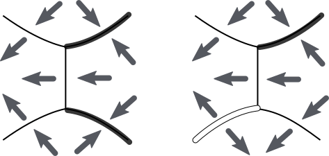
Figure 2. The figure showing how the orientation of the Reeb graph affects the positivity on a component of $K_{\Psi}$: on the left display, all edges of the fat graph component have the Reeb graph orientation pointing toward them, or “through” them; on the right display, the SW edge has both adjacent edges of the Reeb graph outgoing, resulting in locally negative mass. (Positive charges are shown as fat solid lines, negative, - as fat hollow line.)

We remark that Lemma 8 turns the computational question of the positivity of a given gradient quadratic differential $\Psi$ into an instance of a $2$-satisfiability problem, [16]. Indeed, one can interpret the orientations of the edges of the Reeb graph as Boolean variables, and the absence of two outgoing edges of the Reeb graph incident to an edge of a fat graph $K_{\alpha}$ as a $2$-clause. Such interpretation implies that given the fat graph structures, the positivity can be efficiently decided in time quadratic in the number of the critical points of $\Psi$.

The natural length element $|d\Im\sqrt{\Psi}|$ on the edges of the fat graphs $K_{\alpha}$’s (or critical trajectories of $\Psi$) defines the widths on the boundary components of the fat graphs $K_{\alpha}$, or, equivalently, on the edges of the Reeb graph $\mathit{Rg}_{\Psi}.$ (Recall that the lengths of the edges of the Reeb graph are defined by $|d\Re\sqrt{\Psi}|$.) For the components containing poles of $\Psi$ in their closure, the width can be infinite.

Next result is immediate:

Lemma 9.

The total mass of $\mu_{F}$ supported by a component $K_{\alpha}$ equals to the difference of the widths of all incoming and all outgoing components.

Lemma 9 implies the following necessary condition of positivity:

Corollary 1.

If a potential $F$ is positive, then for any component $K_{\alpha}$, the total width of the incoming edges is greater than or equal to the total width of the outgoing edges.

It is worth mentioning that the latter condition is not sufficient: just fixing the Reeb graph of a gradient quadratic differential, and widths and orientations of its edges is not enough to determine the positivity of the corresponding potential. Indeed, the Dehn twists acting on the space of the corresponding complex structures of the Riemann surface $Y$ do not preserve positivity, see Fig. 3.

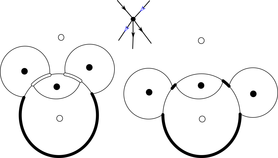
Figure 3. Singular sets and trajectories of clean quadratic differ- entials on ${{\mathbb{C}}{\rm P}}^{1}$ with 5 poles of order 2, and 6 simple zeros each. The residues of the poles (equal to the widths of the circle domains centered at these poles) are the same for corresponding poles on the left and on the right pictures. Yet the potentials on the left has negative components of $\mu_{F}$; the one on the right is positive. The Reeb graph is sketched on the top. (We keep the convention that positive masses are shown as solid lines or dots; negative, - as hollow ones.)

Another constraint on the orientation of the edges of the Reeb graph required by the positivity of a potential comes from the simple poles of $\Psi$, see Fig. 4. As the edge of the fat graph adjacent to a simple pole has the same domain on both sides, the positivity implies that the orientation of the edge of the Reeb graph should be incoming, comp. Proposition 2, [22].

Figure 4. Positivity forces the orientation of the potential function near a simple pole of $\Psi$.

6. Appendix I. Quadratic differentials and Heine-Steiltjes theory

We have earlier encountered Strebel and gradient differentials in the study of the asymptotic properties of Van Vleck and Heine-Stieltjes polynomials and solutions of Schrödinger equation with polynomial potential, see [9, 22, 21]. Some of these results are presented below and they were a major motivation for the present study.

Given a pair of polynomials $P(z)$ and $Q(z)$ of degree $m$ and at most $m-1$ respectively, consider the differential equation:

$$P(z)S^{\prime\prime}(z)+Q(z)S^{\prime}(z)+V(z)S(z)=0.$$ (6.1)

The classical Heine-Stieltjes problem for equation (6.1) asks for any positive integer $n,$ to find the set of all possible polynomials $V(z)$ of degree at most $m-2$ such that (6.1) has a polynomial solution $S(z)$ of degree $n$, see [8], [25]. Already E. Heine proved that for a generic equation (6.1) and any positive $n,$ there exist $\binom{n+l-2}{l-2}$ polynomials $V(z)$ of degree $l-2$ having the corresponding polynomial solution $S(z)$ of degree $n$. Such polynomials $V(z)$ and $S(z)$ are referred to as Van Vleck and Heine-Stieltjes polynomials respectively. The following localization result for the zero loci of $S(z)$ and $V(z)$ was proven in [20].

Proposition 6.

For any $\epsilon>0,$ there exists $N_{\epsilon}$ such that all roots of $V(z)$ and its corresponding $S(z)$ lie within $\epsilon$-neighbourhood of $Conv_{P}$ if $\deg S(z)\geq N_{\epsilon}$. Here $Conv_{P}$ stands for the convex hull of the zero locus of the leading coefficient $P(z)$.

The above localization result implies that there exist plenty of converging subsequences $\{\tilde{V}_{n}(z)\}$ where $V_{n}(z)$ is some Van Vleck polynomial for equation (6.1) whose Stieltjes polynomial $S_{n}(z)$ has degree $n$ and $\tilde{V}_{n}(z)$ is the monic polynomial proportional to $V_{n}(z)$. (Convergence is understood coefficient-wise.)

Recall that the Cauchy transform $\mathcal{C}_{\nu}(z)$ and the logarithmic potential $u_{\nu}(z)$ of a (complex-valued) measure $\nu$ supported in $\mathbb{C}$ are by definition given by:

$$\mathcal{C}_{\nu}(z)=\int_{\mathbb{C}}\frac{d\nu(\xi)}{z-\xi}\quad\text{ and }\quad u_{\nu}(z)=\int_{\mathbb{C}}\log|z-\xi|{d\nu(\xi)}.$$

Obviously, $\mathcal{C}_{\nu}(z)$ is analytic outside the support of $\nu$ and has a number of important properties, e.g. that

$$\mathcal{C}_{\nu}(z)=\frac{\partial u_{\nu}(z)}{\partial z};\quad\quad\nu=\frac{1}{\pi}\frac{\partial\mathcal{C}_{\nu}(z)}{\partial\bar{z}}$$

where the derivative is understood in the distributional sense. Detailed information about Cauchy transforms can be found in e.g. [6].

Theorem 1.

Choose a sequence $\{V_{n}(z)\}$ of Van Vleck polynomials � where $\deg S_{n}(z)=n$ with converging sequence $\{\tilde{V}_{n}(z)\}\to\tilde{V}(z)$. Then the sequence of root-counting measures $\mu_{n}$ of $S_{n}(z)$ weakly converges to the probability measure $\mu$ whose Cauchy transform $\mathcal{C}_{\mu}(z)$ satisfies a.e. in $\mathbb{C}$ the algebraic equation

$$\mathcal{C}_{\mu}^{2}(z)=\frac{\tilde{V}(z)}{P(z)}.$$

Moreover, the logarithmic potential $u_{\mu}(z)$ of $\mu$ has the property that its set of level curves coincides with the set of closed trajectories of the quadratic differential $-\frac{\tilde{V}(z)dz^{2}}{P(z)}$ which is therefore Strebel.

The Theorem 1 implies further results for arbitrary rational Strebel differentials with a second order pole at $\infty$. (These statements are special cases of the results in § 5.)

Theorem 2 (see Theorem 4, [22]).

Let $U_{1}(z)$ and $U_{2}(z)$ be arbitrary monic complex polynomials with $\deg U_{2}-\deg U_{1}=2$. Then

1. the rational quadratic differential $\Psi=-{U_{1}(z)}dz^{2}/{U_{2}(z)}$ on $\mathbb{CP}^{1}$ is Strebel if and only if there exists a real and compactly supported in $\mathbb{C}$ measure $\mu$ of total mass $1$ (i.e. $\int_{\mathbb{C}}d\mu=1$) whose Cauchy transform $\mathcal{C}_{\mu}$ satisfies a.e. in $\mathbb{C}$ the equation:

   $$\mathcal{C}_{\mu}^{2}(z)={U_{1}(z)}/{U_{2}(z)}.$$ (6.2)

2. for any $\Psi$ as in $\rm(1)$ there exists exactly $2^{d-1}$ real measures whose Cauchy transforms satisfy (6.2) a.e. and whose support is contained in $K_{\psi}$ where $d$ is the total number of connected components in $\mathbb{CP}^{1}\setminus K_{\Psi}$ (including the unbounded component, i.e. the one containing $\infty$). These measures are in $1-1$-correspondence with $2^{d-1}$ possible choices of the branches of $\sqrt{{U_{1}(z)}/{U_{2}(z)}}$ in the union of $(d-1)$ bounded components of $\mathbb{CP}^{1}\setminus K_{\Psi}$.

Concerning measures positive in $\mathbb{CP}^{1}$, with the only non-simple pole at infinity, we notice first, that the Reeb graph is necessarily a tree, with infinite length edges corresponding to the edge domains (adjacent to $\infty\in\mathbb{CP}^{1}$) and with the leaves which correspond to the components of $K_{\Psi}$ containing, necessarily, simple poles of $\Psi$. Given that, the following statement should be quite obvious.

Theorem 3 (see Theorem 5, [22]).

For any Strebel differential $\Psi=-{U_{1}(z)}dz^{2}/{U_{2}(z)}$ on $\mathbb{CP}^{1}$ (in the notation of Theorem 2) there exists at most one positive measure satisfying (6.2) a.e. in $\mathbb{C}$. Its support necessarily belongs to $K_{\Psi}$, and, therefore, among $2^{d-1}$ real measures described in Theorem 2 at most one is positive.

Moreover, we can formulate an exact criterion of the existence of a positive measure in terms of rather simple topological properties of $K_{\Psi}$. To do this we need one more definition. Observe that in our situation $K_{\Psi}$ is a planar multigraph.

Definition 9.

By a simple cycle in a planar multigraph $K_{\Psi},$ we mean any closed non-self-intersecting curve formed by the edges of $K_{\Psi}$. (Obviously, any simple cycle bounds an open domain homeomorphic to a disk which we call the interior of the cycle.)

Proposition 1 (see Proposition 2, [22]).

A Strebel differential $\Psi=-{U_{1}(z)}dz^{2}/{U_{2}(z)}$ admits a positive measure satisfying (6.2) if and only if no edge of $K_{\Psi}$ is attached to a simple cycle from inside. In other words, for any simple cycle in $K_{\Psi}$ and any edge not in the cycle but adjacent to some vertex in the cycle this edge does not belong to its interior. The support of the positive measure coincides with the forest obtained from $K_{\Psi}$ after the removal of all its simple cycles.

References

- [1] Yu. Baryshnikov, On Stokes sets, in “New developments in singularity theory (Cambridge, 2000)”, 65–86, NATO Sci. Ser. II Math. Phys. Chem., Vol. 21, Klüwer Acad. Publ., Dordrecht, (2001).
- [2] J. Borcea, R. Bøgvad, Piecewise harmonic subharmonic functions and positive Cauchy transforms, Pac. J Math., vol. 240, no. 2, pp. 231–265, 2009.
- [3] ï H. Federer, Geometric measure theory, Die Grundlehren der mathematischen Wissenschaften, Band 153 Springer-Verlag New York Inc., New York 1969 xiv+676 pp.
- [4] M. Fedoruyk, Asymptotic analysis. Linear ordinary differential equations. Springer-Verlag, Berlin, viii+363 pp, (1993).
- [5] F. P. Gardiner, The existence of Jenkins-Strebel differentials from Teichmüller theory, Amer. J. Math., (99:5), (1977), 1097–1104.
- [6] J. Garnett, Analytic capacity and measure, LNM 297, Springer-Verlag, 1972, 138 pp.
- [7] P. Griffiths, J. Harris, Principles of algebraic geometry. Reprint of the 1978 original. Wiley Classics Library. John Wiley & Sons, Inc., New York, 1994. xiv+813 pp.
- [8] E. Heine, Handbuch der Kugelfunktionen, Berlin: G. Reimer Verlag, (1878), vol.1, 472–479.
- [9] T. Holst, and B. Shapiro, On higher Heine-Stieltjes polynomials, Isr. J. Math. 183 (2011) 321–347.
- [10] L. Hörmander, The analysis of linear partial differential operators. I. Distribution theory and Fourier analysis. Reprint of the second (1990) edition. Classics in Mathematics. Springer-Verlag, Berlin, 2003.
- [11] G. A. Jones, and D. Singerman, Theory of maps on orientable surfaces, Proc. London Math. Soc. (3), 37, (1978), 273–307.
- [12] J. A. Jenkins, Univalent functions and conformal mapping. Ergebnisse der Mathematik und ihrer Grenzgebiete. Neue Folge, Heft 18. Reihe: Moderne Funktionentheorie Springer-Verlag, Berlin-Göttingen-Heidelberg 1958 vi+169 pp.
- [13] P. Lelong, Fonctions plurisousharmoniques et formes différentielles positives, Gordon and Breach, Paris-London-NY, 1968.
- [14] A. Martínez-Finkelshtein, E. A. Rakhmanov, Critical measures, quadratic differentials, and weak limits of zeros of Stieltjes polynomials, Commun. Math. Phys. vol. 302 (2011) 53–111.
- [15] A. Martínez-Finkelshtein, E. A. Rakhmanov, On asymptotic behavior of Heine-Stieltjes and Van Vleck polynomials, Contemp. Math. vol. 507, (2010) 209–232.
- [16] C. Moore, St. Mertens, The Nature of Computation OUP Oxford, 985 pp. (2011).
- [17] I. Pritsker, How to find a measure from its potential, CMFT, vol. 8(2), 2008, 597–614.
- [18] T. Ransford, Potential Theory in the Complex Plane, LMS Student Texts 28, Cambridge University Press, 1995.
- [19] E. B. Saff, V. Totik, Logarithmic potentials with external fields, Springer-Verlag, Berlin, (1997).
- [20] B. Shapiro, Algebro-geometric aspects of Heine-Stieltjes theory, J. London Math. Soc. 83(1) (2011) 36–56.
- [21] B. Shapiro, On Evgrafov-Fedoryuk’s theory and quadratic differentials, Anal. Math. Phys. vol 5 (2015) 171–181.
- [22] B. Shapiro, K. Takemura, M. Tater, On spectral polynomials of the Heun equation. II, Comm. Math. Phys. 311(2) (2012), 277–300.
- [23] H. Stahl, Extremal domains associated with an analytic functions. I, II, Compl. Var. Th. Appl., vol. 4(4), 311–324, 325-338, (1985).
- [24] K. Strebel, Quadratic differentials. Ergebnisse der Mathematik und ihrer Grenzgebiete (3) [Results in Mathematics and Related Areas (3)], 5. Springer-Verlag, Berlin, 1984. xii+184 pp.
- [25] T. J. Stieltjes, Sur certains polynomes qui vérifient une équation différentielle linéaire du second ordre et sur la theorie des fonctions de Lamé. Acta Math. 6 (1885), no. 1, 321–326.
- [26] R. O. Wells, Differential analysis on manifolds, Prentice-Hall Inc, NJ, 1973.