The shapes of nuclei

Abstract

Gerry Brown initiated some early studies on the coexistence of different nuclear shapes. The subject has continued to be of interest and is crucial for understanding nuclear fission. We now have a very good picture of the potential energy surface with respect to shape degrees of freedom in heavy nuclei, but the dynamics remain problematic. In contrast, the early studies on light nuclei were quite successful in describing the mixing between shapes. Perhaps a new approach in the spirit of the old calculations could better elucidate the character of the fission dynamics and explain phenomena that current theory does not model well.

I Introduction

In the early 1960’s, Bohr and Mottelson pointed out some puzzling experimental data: some light nuclei thought to be spherical in shape had excited energy levels exhibiting characteristics of deformed nuclei. This was taken up first by Engeland en65 and then Gerry Brown, who saw an opportunity to test the realistic nuclear interactions that were being developed at the time. The nuclei ¹⁶O and ¹⁸O were the first subjects of study br66 . As his graduate student, I worked on a parallel study of Ca isotopes as part of my thesis project. Later, a more definitive study of the Ca nuclei was carried out by Gerace and Green ge67 . As a general conclusion, one saw that the mixing between shapes could be understood with the realistic interactions derived from nucleon-nucleon scattering data.

Since those early days of nuclear structure physics, the subject of nuclear deformation has matured. First of all, we now know that the shape coexistence is ubiquitous in the low-energy spectra of nuclei across the periodic table, affecting even the fission properties of the heaviest nuclei. Also, we now have computational tools to describe and predict the static features of the landscape of nuclear shapes. However, the dynamics of shape change, ie. how different shapes mix together, has been a challenging problem in the theory of heavy nuclei and is still not well understood. I shall describe some work I have been engaged in recently, to develop a new approach to fission dynamics in the spirit of the old studies on light nuclei.

II Theory of static deformations

Nuclei are highly deformable, and the first task is to construct reliable models of the nuclear potential energy surface, ie. the energy of configurations as a function of deformation coordinates such as the expectation values of quadrupole and higher moments. An immediate question is how to define both energy and shape of a configuration: the operators for these two quantities do not commute. The resolution of this conundrum is that we are only dealing with approximate wave functions, not the true eigenstates of the Hamiltonian. In practice, theory relies on the mean-field representation of wave functions as products of single-particle orbitals. The present-day calculational framework is very similar to the Density Functional Theory (DFT) of condensed matter physics. One defines an effective interaction, which may depend on the local density. The energies and shapes are determined by minimizing the energy expectation value just as in Hartree-Fock (HF) theory.

Several families of DFT in use today, and all have considerable predictive power on static properties of nuclei. In the examples discussed below, I will show results obtained with the Gogny D1S functional. de10 . It has 14 parameters, 3 of them fixed and 11 adjusted many years ago D1S to reproduce general nuclear properties. An example showing its considerable predictive power is recent systematic study of the low-energy spectroscopy of even-even nuclei de10 . I will come back to findings from this study later. Another success of the DFT approach is verification of additional shape minima at very high deformation in heavy nuclei. The potential energy surface that a fissioning nucleus traverses has at least two minima and perhaps more. Fig. 1 shows the energy versus deformation in a typical fissile nucleus.

Figure 1: Potential energy surface for ²³⁶U covering the range of deformations up to the scission point. The curve was calculated by minimizing the D1S density functional with the mass quadrupole moment constrained to the value on the abscissa. The point marked “I” is the global minimum. The points marked “A” and “B” are saddle points on the fission path, with a second minimum “II” in between.

III How nuclei change shape

Up to now, the only practical approach for treating shape dynamics in heavy nuclei is the Generator Coordinate Method (GCM) proposed by Hill and Wheeler hi53 . Formally, one generates a continuum of configurations by minimizing the Hamiltonian in the presence of an external field. Thus, the configuration $|\Psi_{\lambda}\rangle$ is defined by minimizing

$$\langle\Psi_{\lambda}|\hat{H}-\lambda\hat{Q}|\Psi_{\lambda}\rangle$$ (1)

where $\hat{H}$ is the Hamiltonian or energy-density functional and $\hat{Q}$ is a one-body operator such as the axial quadrupole field

$$\hat{Q}_{20}=\hat{z}^{2}-(\hat{x}^{2}+\hat{y}^{2})/2.$$ (2)

Then one constructs an effective Hamiltonian from information about the diagonal and off-diagonal matrix elements $\langle\Psi_{\lambda}|\Psi_{\lambda}^{\prime}\rangle$ and $\langle\Psi_{\lambda}|\hat{H}|\Psi_{\lambda}^{\prime}\rangle$.

Computationally, the GCM can be implemented in two ways. In the first way, the moment $q=\langle\Psi_{\lambda}|\hat{Q}|\Psi_{\lambda}\rangle$ is treated as the position variable in a one-dimensional Schrödinger equation. It is straightforward to derive formulas for potential energy function $V(q)$ and a kinetic energy operator

$$-{1\over 2}{\partial\over\partial q}{1\over{\cal I}(q)}{\partial\over\partial q}$$ (3)

in approximations such as the Gaussian Overlap Approximation gi83 . This one-dimensional collective approach works well for treating the ground state tunneling under the barriers, but generalizing it to include excited states is cumbersome be11 . A more technical problem is necessity to define at least four or five deformation operators to completely specify the shape of the fissioning nucleus. It is possible, but not easy, to set up and solve the corresponding higher-dimension Schrödinger equation; a two-dimensional approximation was carried out in Ref. go05 .

The second computational method is to discretize the GCM configurations with a mesh of $\lambda$ values and minimize the Hamiltonian in that finite basis. There are obstacles to this approach as well. On a purely technical level, the fact that the configurations are not orthogonal leads to numerical instabilities. More serious on a fundamental level, it is not clear how to calculate interaction matrix elements between configurations when they are constructed via an energy density functional. Several plausible prescriptions are possible, but the results can be unphysical if the wrong prescription used ro10 . Such problems never occurred in the early work on light nuclei—we used orthogonal bases and we had a pretty good idea of the interactions.

To build an alternative to the GCM approach, we should start by constructing an orthonormal basis within the mean-field framework. The dynamics can be developed later from the off-diagonal interactions in this basis. In the old work, the basis was constructed from the harmonic oscillator Hamiltonian by using the associated SU(3) group structure to organize the many-body configurations. This is obviously too crude for treating heavy nuclei, and it is better to use the DFT to build the orbitals. In the nuclear context, one could use DFT orbitals and still preserve orthogonality by to constraining them by their quantum numbers rather than by their deformations. For most nuclei, the mean-field potential is axially symmetric and has good parity at the DFT minima. This allows one to assign orbital quantum numbers $K^{\pi}$, where $K$ is the angular momentum about the symmetry axis and $\pi$ is the parity of the orbital. The DFT minimization can be carried out taking as a constraint the number of nucleons having given values of $K$, $\pi$, and isospin projection $\tau_{z}$. Wave functions that differ in filling numbers are automatically orthogonal, so this should be very helpful for constructing an orthogonal basis. In the remaining sections of this article, I will go through some examples illustrating the use of a $K^{\pi}$ partitioning to define the configurations.

Before going on to the examples, it is instructive to see how the partitioning works in a semiclassical limit. Assume that the nucleus is spherical and the phase space density is uniform in spheres of radius $R$ in coordinate space and $k_{F}$ in momentum space. Then the number of nucleons having orbital quantum number $M$ is given by

$$n_{M}=g\int^{R}d^{3}r\int^{k_{F}}{d^{3}k\over(2\pi)^{3}}\delta(M-(\vec{r}\times\vec{k})_{z})$$ (4)

where $g=2$ is the spin degeneracy of the nucleon and $M$ is the orbital angular momentum about the $z$-axis. The integrals can be carried out analytically; the result is

$$n_{M}={9N\over 4k_{F}R}\left((1/2+x^{2}){\rm arccos}\,x-3x(1-x^{2})^{1/2}\right)$$ (5)

where $x=M/(k_{F}R)$. The same formula applies to ellipsoidally deformed nuclei with the radius $R$ replace by the transverse radius of the ellipsoid. Fig. 2 shows the distribution for the neutrons in the spherical nucleus ²⁰⁸Pb, comparing the mean-field fillings with the formula (5).

Figure 2: $M$ distribution of occupied neutron orbitals in the nucleus ²⁰⁸Pb. Histogram: spherical shell model. Dashed line Eq. (5 with $R=7.1$ fm, $k_{F}=1.35$ fm^-1.

IV Examples

The shells of the three-dimensional harmonic oscillator model are completely filled or empty at nucleon numbers 8, 20, 40,… The first two examples here are nuclei at those possibly magic numbers: ⁴⁰Ca  and ⁸⁰Zr. The third example deals with the early shape changes in a fissioning ²³⁶U nucleus.

IV.1 ⁴⁰Ca

The spectroscopy of ⁴⁰Ca has been known since the early 1960’s. Fig. 3 shows the states in the spectrum that are relevant to the discussion.

Figure 3: The spectrum of ⁴⁰Ca, showing the first three levels of the deformed band and the gamma transitions that establish the deformation of the band ma71

The first excited state in the spectrum has angular moment zero, which is rare among the 600 or so known even-even nuclei. The excited $0^{+}$ together with the $2^{+}$ and $4^{+}$ above it form the lowest members of a rotational band. The evidence that these states are part of a band comes from the energy spacing and from the electromagnetic transition rates between states, indicated by arrows in the Figure. The measured quadrupole transition strength between two lowest states in the band is $B(E2,2^{+}_{1}\!\rightarrow\!{0^{+}_{2}})=250\pm 35$ e² fm⁴ ma71 . On the scale of a single-particle quadrupole moment this is very large and would require an axis ratio of $a_{z}/a_{\perp}\approx 1.55$ to model the band as an ellipsoidal rotor. The corresponding intrinsic mass quadrupole moment in the band is

$$\langle\,\hat{Q}_{20}\,\rangle=117~{}~{}{\rm fm}^{2}.$$ (6)

Now let us compare the GCM and the $K^{\pi}$-partition approaches to determine the structure of the band. We start with the GCM, applying a field $\lambda\hat{Q}_{20}$ to the spherical ground state configuration. The minimization is performed small increments of $\lambda$ up to the point where the configuration has the deformation (6) extracted from experiment. The results are shown in Fig. 4 as the open circles.

Figure 4: Energies of ⁴⁰Ca configurations calculated by the GCM (open circles) and by $K^{\pi}$-constrained minimization (black circle).

The energy increases monotonically as the deformation increases. At the deformation corresponding to the one extracted from experiment, the excitation energy is 13 MeV. This is way off from the observed band head at 3.35 MeV. There will be a small gain of energy when one takes into account that the calculated energy is that of the band as a whole, but the energy gain is probably too small to approach the experimental value. Anyway, a big surprise comes when we look at the shape of the nucleus, shown as in the middle panel of Fig. 5. One sees that the GCM-generated configuration no longer has good parity; there is a strong octupole component as well as the quadrupole deformation. This would imply that the band should have odd-parity members interleaved between the even-parity members. Since that is not the case, so we can concluded that GCM carried out this way has failed.

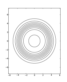
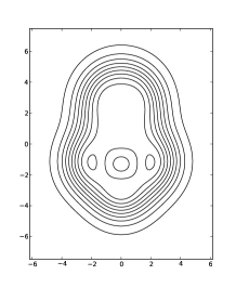
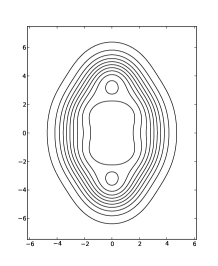
Figure 5: Density distribution of the ⁴⁰Ca configurations. Left: ground state; center: GCM configuration at $q=108$ fm²; right: 4p-4h $K^{\pi}$-constrained configuration.

Now let’s try the $K^{\pi}$-constrained approach using the $K^{\pi}$ partitions from Ref. ge67 . The ground state configuration has the fillings of the spherical shell model. The deformed configuration was built by taking the lowest 4-particle 4-hole excited state in a deformed harmonic oscillator potential. This is the Nilsson model; its diagram of orbital energies is shown in Fig. 6. We carry out the DFT minimization again, but now use the $K^{\pi}$ quantum numbers of the occupied orbitals to constrain the minimization. The results for the spherical and deformed configurations are shown in Fig. 4 as the black square and black circle, respectively. The predicted quadrupole moment of the deformed configuration, 105 fm², agrees well with (6). The energy is still too high, but it is lower than the GCM energy and so is a better candidate for understanding the band structure. Of course, one can obtain the configuration by GCM minimization, but doing this would require a different starting point or additional shape-dependent constraints. One final point: as may be seen in the right-hand panel of Fig. 5, the configuration found by starting from the 4p-4h hole configuration preserves the even parity of the band.

Figure 6: Single-particle energies of orbitals around the Fermi level of ⁴⁰Ca as a function of deformation. The deformed band is attributed to 4-particle 4-hole excitation shown with solid and open circles (after Fig. 1 of Ref. ge67 .

Ignoring the energy problem, one can try to calculate the mixing of deformed and spherical states, as was done by the early researchers. Unfortunately, as I mentioned earlier, there is no consistent way to extract configuration-interaction elements from a DFT. But DFT should still be useful to construct the configurations. The Hamiltonian matrix elements might be evaluated using these configurations as in the condensed-matter hybrid procedure.

IV.2 ⁸⁰Zr region

At the next harmonic oscillator shell closure ($N=20$ at ⁸⁰Zr), the competition between spherical and deformed configurations plays out differently. The coexistence question here was addressed in the DFT by Zheng and Zamick zh91 . They tried several energy functionals in the Skyrme family and found that a deformed configuration came out lower than the spherical. While in ⁴⁰Ca there were 4 particle jumps needed to connect the configurations, 12 jumps were needed in ⁸⁰Zr. The Gogny D1S functional yields rather similar results. The corresponding potential energy surface is shown in Fig. 7. The filled square and circle show the minima for the spherical and deformed configurations, obtained by constraining the $K^{\pi}$ partitions according to the spherical shell model and the 12p-12h Nilsson configuration. The latter has a very large deformation, $Q_{20}\approx 400$ fm², at an energy $~{}3.5$ MeV above the global minimum. The deformation is very robust with respect to the choice of energy functional. In terms of the dimensionless deformation parameter $\beta$, the Skyrme functionals and the Gogny D1S all give $\beta=0.44\pm 0.01$. The authors of Ref. zh91 also note that a simple formula derived earlier by myself is quite accurate.

The energetics are more complicated. First of all, the shell model configuration is not the lowest energy minimum at $q=0$. The actual minimum has broken parity with a large octupole moment and a very small quadrupole moment. The entire potential energy surface up to high deformation can be generated by GCM procedure, provided one starts with a configuration that already has an octupole deformation. It is shown as the solid line in the Figure.

Figure 7: The ⁸⁰Zr potential energy surface. The solid line is generated by the GCM procedure, starting from a octupole-deformed ground state minimum. The $K^{\pi}$-constrained minimization starting from the partition of the spherical shell model configuration is shown at the black square. Starting with the 12p-12h partitions gives the filled circle, coinciding with the second minimum of the GCM potential energy curve.

While the 12p-12h is not the lowest configuration in the Gogny DFT, correlation effects can change the ordering. Recently de10 a systematic study of low-energy spectroscopy was carried out including all five quadrupole shape degrees of freedom in the GCM framework. In that way, rotational energies and some shape mixing effects are taken into account. As an example of the predictive power of the Gogny functional and the method, it was found that calculated quadrupole transition moments of deformed nuclei agree with experiment to $~{}10\%$ accuracy. For the ⁸⁰Zr nucleus, the authors found that the rotational energy was enough to bring the band head of the highly deformed configuration down to the ground state. Fig. 8 compares their calculated $2^{+}$ excitation energies across the chain of the heavy $N=Z$ even-even nuclei. One sees that $2^{+}$ excitation energy in ⁸⁰Zr agrees very well with experiment. It is also the most highly deformed in the chain, judging by the excitation energy of the lowest $2^{+}$ state. The heaviest measured nucleus in the Figure, ⁹⁶Pd, is a real prediction, as the experimental measurement ce11 was reported the following year. So, despite the mixed performance of DFT in ⁴⁰Ca, we find that the energy functionals becomes quite successful in a heavier region of nuclei.

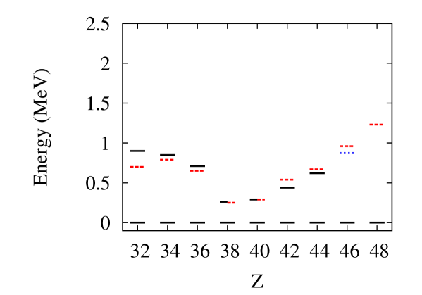
Figure 8: Systematics of $2^{+}$ excitations in the heaviest known $N=Z$ nuclei. Solid black lines: older experiments; red dashed line: Gogny/GCM theory de10 . Theory and experiment are visually indistinguishable for the nuclei ⁷⁶Sr and ⁸⁰Zr. The blue dotted line shows the new measurement at ⁹⁶Pd ce11 .

V Fission dynamics

My ultimate goal is to gain a better understanding of the dynamics of fissioning nuclei. As mentioned at the beginning, the GCM approach works well for describing spontaneous fission as tunneling through a barrier in the potential energy surface. But when the excitation energy is above the barrier, it is far from clear what theoretical approach is justified. In any case, the spontaneous fission show that the part of the interaction responsible for pairing is very important ro14 . This suggests that the time-dependent Hartree-Fock-Bogoliubov approximation (TD-HFB) might be appropriate for above-barrier dynamics. Recently, computer power has become available to test the TD-HFB for fission using current nuclear energy functionals. Such a study was carried out by Bulgac and collaborators bu16 . Their starting point was a very deformed configuration past the second barrier and at a small excitation energy over the potential energy surface. They found that fission would take place, but the duration before the fragment formation could be very long.

A weak point of the TD-HFB approximation is that it takes into account only a very restricted set of interaction matrix elements to propagate the system from one configuration to another. Namely, configurations that can be generated as two-quasiparticle excitations of the starting configuration are included in some way, but all four-quasiparticle transitions are neglected. In the example of configuration mixing in ⁴⁰Ca, the HFB approximation would be useless. There is no pairing condensate, and even if there were one, the intermediate configurations are only partially represented by the allowed pair jumps.

While it would still be an enormous challenge to make a realistic treatment of fission in the discrete-configuration approach, we can at least see how the landscape could be traversed. We concentrate on the two minima and the barrier between them. Fig. 9 shows the potential energy surface of ²³⁶U again, expanding the horizontal scale in the region of the first barrier.

Figure 9: ²³⁶U HFB potential energy surface between the first and second minima and the energies of the partition-constrained HF wave functions. Solid and dashed lines are the HF and HFB potential energy surfaces respective. Diamonds show the energy and quadrupole moment of the partition-constrained minima.

Figure 10: Path from the first to second minimum in the $(q_{20},q_{40})$ plane. The left-hand panel shows the HFB energies constrained by $q2$. The minima and intermediate maximum are marked by filled circles. The right-hand panel shows the same path in the HF approximation. The filled diamonds are the partition-constrained minima. In principle, either method should produce the same global minimum.

The lower curve was obtained by the GCM in the HFB approximation, which includes pairing effects. The more jagged curve above that is the GCM in the HF, ie. ignoring pairing effects. The HF configurations have definite $K^{\pi}$ partitions that change abruptly along the curve. The black dots are three configurations generated by the $K^{\pi}$-constrained minimization, with the partitions taken from the GCM results. It is interesting to compare the $K^{\pi}$ partitions found with the Gogny D1S energy function with other simpler ways for building a many-particle wave function. The simplest is the Nilsson model mentioned earlier. One finds that it gives exactly the same ground state $K^{\pi}$ partition as the DFT. Another model simpler than the DFT is the Finite-Range Liquid Drop Model mo09 . Here the orbital energies are computed in a deformed potential well, but the shape of the well is determined by an energy functional based in part on the liquid drop model. It also gives the same $K^{\pi}$ partition as the other models. This suggests that the $K^{\pi}$ filling of the ground state is a quite robust property of the mean-field wave function. And it is certainly easier to specify, compared with the many shape parameters needed to describe unambiguously configurations obtained by the GCM. However, at the A and the II points along the fission path the partition obtained with the Gogny functional differs by one pair jump from the FRLD partition. It is likely that they are nearly degenerate, and would be mixed by the pairing interaction.

For dynamics, an important consideration is the number of steps it takes to get from one configuration to another via the two-particle interaction in the Hamiltonian. This suggests a distance measure between configurations as the number of pairing jumps needed to get from one to the other. Fig. 10 shows a plot of the path from configuration I to II via the barrier top at A, showing both the quadrupole and hexadecapole coordinates of the intermediate configurations. The left-hand plot is the GCM in the HFB approximation, which is seen to be smooth with very little structure. The right-hand plot shows the same path in the HF approximation. It is broken into a sequence of segments, each segment having a specific $K^{\pi}$ partition. Analyzing these segments, one can determine that it takes 6 pair jumps to get from I to A and 8 pair jumps to get from A to II. But it would wrong to concluded that it takes 14 pair jumps to get from I and II. In fact, examination of end-points reveals that the configuration II can be reached from I by changing the orbits of only 6 pairs. That of course requires surmounting a higher potential barrier. Which path is more important in the dynamics is not obvious; one needs to know interaction matrix elements between configurations as well as their energies to begin to address this question.

VI Conclusion

The configuration-interaction method has been very successful in light nuclei, and it should be possible, at least in a statistical way, to extend it to heavy nuclei. I have concentrated exclusively on the basis of wave functions, advocating the use of DFT constrained by $K\pi$ partitioning. This still leaves the interaction matrix elements to be determined. The same problem exists in condensed-matter theory, and there a hybrid approach has been quite successful sa16 .

It would take a large effort to carry out this program in nuclear physics. However, there are good reasons, rooted in experimental findings, to undertake that effort. Empirically, there is strong evidence that the fissioning nucleus is close to a statistical equilibrium near the scission point ra11 . The big open theoretical question is whether we can explain that in terms of Hamiltonian dynamics with realistic interactions.

Fluctuation phenomena also remain unexplained. Here are two examples. In 1978 Keyworth and collaborators measured the fission cross sections for neutron-induced fission of ²³⁵U separating out the individual angular momentum channels. Besides the fluctuations associated with the compound nucleus states near the waypoints I and II, they saw fluctuations on much larger energy scale mo78 . The data for one of the angular channels is shown in Fig. 11.

Figure 11: Average fission width of the $J=4$ compound-nucleus states in ²³⁶U as a function of excitation energy. The dashed line is the predicted width from the Bohr-Wheeler theory with one open channel. The solid curve is a fit to the experimental data in Ref. mo78 .

It may be that the discrete states near the barrier tops are responsible. A discrete basis would be very helpful here.

Another old experiment exhibiting unexplained fluctuations is the measurement of angular distributions of fission fragments by Huizenga, Loveland, and collaborators be69 . The distributions very close to threshold could be fitted with the usual theory, but on examination of a more extended range they found: “Further attempts to fit the data… were unsuccessful.”

In summary, I think there is a good case for trying a discrete configuration approach to shape dynamics in heavy nuclei as an alternative to the GCM.

References

- (1) T. Engeland, Nucl. Phys. 72 68 (1965).
- (2) G.E. Brown and A.M. Green, Nucl. Phys. 75 401 (1966).
- (3) W.J. Gerace and A.M. Green, Nucl. Phys. A 93 110 (1967).
- (4) J.P. Delaroche, et al., Phys. Rev. C81 014303 (2010).
- (5) J.F. Berger M. Girod and D. Gogny, Comp. Phys. Comm. 63 365 (1991).
- (6) D.L. Hill and J.A. Wheeler, Phys. Rev. 89 1102 (1953).
- (7) M. Girod and B. Grammaticos, Phys. Rev. C 27 2317 (1983).
- (8) R. Bernard, H. Goutte, D. Gogny and W. Younes, Phys. Rev. C 84 044308 (2011).
- (9) H. Goutte, et al., Phys. Rev. C 71 024316 (2005).
- (10) L.M. Robledo, J. Phys. G 37 064020 (2010).
- (11) J.R. MacDonald, et al., Phys. Rev. C 3 219 (1971).
- (12) D.C. Zheng and L. Zamick, Phys. Lett. B 266 5 (1991).
- (13) B. Cederwall, et al., Nature 469 68 (2011).
- (14) R. Rodigruez-Guzman and L.M. Robledo, Phys. Rev. C 89 054310 (2014).
- (15) A. Bulgac, et al., Phys. Rev. Lett. 116 122504 (2016).
- (16) P. Möller, et al., Phys. Rev. C 79 064304 (2009).
- (17) D. Sangalli, et al., arXiv:1603.00225 (2016).
- (18) J. Randrup and P. Möller, Phys. Rev. Lett. 106 132503 (2011).
- (19) M.S. Moore, et al., Phys. Rev. C 18 1328 (1978)l.
- (20) A. Behkami, et al., Phys. Rev. 171 1267 (1969).