Cost-Sensitive Reference Pair Encoding for Multi-Label Learning

Abstract

Label space expansion for multi-label classification (MLC) is a methodology that encodes the original label vectors to higher dimensional codes before training and decodes the predicted codes back to the label vectors during testing. The methodology has been demonstrated to improve the performance of MLC algorithms when coupled with off-the-shelf error-correcting codes for encoding and decoding. Nevertheless, such a coding scheme can be complicated to implement, and cannot easily satisfy a common application need of cost-sensitive MLC—adapting to different evaluation criteria of interest. In this work, we show that a simpler coding scheme based on the concept of a reference pair of label vectors achieves cost-sensitivity more naturally. In particular, our proposed cost-sensitive reference pair encoding (CSRPE) algorithm contains cluster-based encoding, weight-based training and voting-based decoding steps, all utilizing the cost information. Furthermore, we leverage the cost information embedded in the code space of CSRPE to propose a novel active learning algorithm for cost-sensitive MLC. Extensive experimental results verify that CSRPE performs better than state-of-the-art algorithms across different MLC criteria. The results also demonstrate that the CSRPE-backed active learning algorithm is superior to existing algorithms for active MLC, and further justify the usefulness of CSRPE.

1 Introduction

The multi-label classification (MLC) problem aims to map an instance to multiple relevant labels [1, 2], which matches the needs of many real-world applications, such as object detection and news classification. Different applications generally require evaluating the performance of MLC algorithms with different criteria, such as the Hamming loss, 0/1 loss, Rank loss, and F1 score [3].

Most existing MLC algorithms are designed to optimize one or few criteria. For instance, binary relevance (BR) [3] learns a binary classifier per label to predict its relevance, and naturally optimizes the Hamming loss. Classifier chain (CC) [4] extends BR by ordering the labels as a chain and using earlier labels of the chain to improve the per-label prediction, and optimizes the Hamming loss like BR. Label powerset (LP) [3] optimizes the 0/1 loss by solving a multi-class classification problem that treats each label combination as a hyper-class. These cost-insensitive algorithms cannot easily adapt to different criteria, and may suffer from bad performance when evaluated with other criteria.

Cost-sensitive MLC (CSMLC) algorithms are able to adapt to different criteria more easily. In particular, CSMLC algorithms take the criterion as an additional piece of input data and aim to optimize the criterion during the learning process. Two state-of-the-art CSMLC algorithms are probabilistic classifier chain (PCC) [5] and condensed filter tree (CFT) [6]. PCC estimates the conditional probability of the labels to infer the Bayes-optimal decision with respect to the given criterion. While PCC can tackle any criterion in principle, the Bayes-optimal inference step can be time-consuming unless an efficient inference rule of the criterion is derived in advance. CFT can be viewed as an extension of CC for CSMLC by re-weighting each example with respect to the criterion when training each binary classifier. Nevertheless, the re-weighting step depends on going back and forth within the chain, making CFT still somewhat time-consuming and hardly parallelizable.

The multi-label error-correcting code (ML-ECC) [7] framework is a more sophisticated algorithm that goes beyond the per-label classifiers to improve classification performance. ML-ECC uses error-correcting code (ECC) to transform the original MLC problem into a bigger MLC problem by adding error-correcting labels during encoding. Classifiers on those labels, much like ECC for communication, can be used to correct prediction errors made from the original per-label classifiers and improve MLC performance. While ML-ECC is successful in terms of the Hamming loss and 0/1 loss [7], it is not cost-sensitive and cannot easily adapt to other evaluation criteria. In fact, extending ML-ECC for CSMLC problem appears to be highly non-trivial and has not yet been deeply studied.

In this work, we study the potential of ECC for CSMLC by considering a special type of ECC, the one-versus-one (OVO) code, which is a popular code for multi-class classification [8]. We extend the OVO code to a cost-sensitive code, cost-sensitive reference pair encoding (CSRPE), which preserves the information of the criterion in each code-bit during encoding. We further propose a method to convert the criterion into instance weights during training, and a method to take the criterion into account during decoding. To make the whole CSRPE algorithm efficient enough to deal with exponentially many possible label vectors, we study the possibility of sampling the code-bits and zooming into a smaller subset of label vectors during prediction. The resulting algorithm is as efficient as a typical random forest (when coupled with decision trees) in training, and can be easily implemented in parallel. Extensive experimental results demonstrate that CSRPE outperforms existing ML-ECC algorithms and the state-of-the-art CSMLC algorithms across different criteria.

In addition, based on the proposed CSRPE, we design a novel algorithm for multi-label active learning (MLAL). Retrieving ground-truth labels is usually expensive in real-world applications [2]. The goal of MLAL is to actively query the labels for a small number of instances while maintaining good test MLC performance. Nevertheless, current MLAL algorithms [9, 10, 11] are not capable of taking the evaluation criterion into consideration when querying. In this paper, we formulate the cost-sensitive multi-label active learning (CSMLAL) setting, and propose a novel algorithm that leverages the code space computed by CSRPE to conduct cost-sensitive querying. Experimental results justify that the proposed algorithm is superior to other state-of-the-art MLAL algorithms.

This paper is organized as follows. First, we define CSMLC problem formally and introduce the ML-ECC framework in Section 2. Our proposed CSRPE algorithm is described in Section 3. In Section 4, we define the CSMLAL problem and solve it with a novel algorithm based on CSRPE. The empirical studies of both CSRPE and its active learning extension are presented in Section 5 . Finally, we conclude the paper in Section 6.

2 Preliminary

The goal of a MLC problem is to map the feature vector $\mathbf{x}\in\mathcal{X}\subseteq\mathbb{R}^{d}$ to a label vector $\mathbf{y}\in\mathcal{Y}\subseteq\{0,1\}^{K}$, where $\mathbf{y}[k]=1$ if and only if the $k$-th bit is relevant. During training, MLC algorithms use the training dataset $\mathcal{D}=\{(\mathbf{x}^{(n)},\mathbf{y}^{(n)})\}_{n=1}^{N}$ to learn a classifier $f\colon\mathcal{X}~{}\to~{}\mathcal{Y}$. During testing, for any test example $(\mathbf{x},\mathbf{y})$ drawn from the distribution that generated $(\mathbf{x}^{(n)},\mathbf{y}^{(n)})$, the prediction $f(\mathbf{x})$ is evaluated with a cost function $C\colon\mathcal{Y}\times\mathcal{Y}\to\mathbb{R}$, where $C(\mathbf{y},\mathbf{\hat{y}})$ represents the penalty of predicting $\mathbf{y}$ as $\mathbf{\hat{y}}$. The objective of MLC algorithms is to minimize the expected cost $\mathbb{E}_{(\mathbf{x},\mathbf{y})}[C(\mathbf{y},f(\mathbf{x}))]$.

Traditional MLC algorithms are designed to optimize one or few cost functions. These algorithms may suffer from bad performance when other cost functions are used. On the contrary, cost-sensitive multi-label classification (CSMLC) algorithms take the cost function as an additional input and learn a classifier $f$ from both $\mathcal{D}$ and $C$. Classifier $f$ should adapt to different $C$ easily.

The multi-label error-correcting code (ML-ECC) [7] framework is originally designed to optimize one cost function (the 0/1 loss). ML-ECC borrows the error-correcting code (ECC) from the communication domain. ML-ECC views the label vectors $\mathbf{y}^{(n)}$ as bit strings and encodes them to longer codes $\mathbf{b}^{(n)}=enc(\mathbf{y}^{(n)})$ with some ECC encoder $enc\colon\mathcal{Y}\to\{0,1\}^{M}$, where $M$ is the code length. An MLC classifier $h$ is trained on $\{(\mathbf{x}^{(n)},\mathbf{b}^{(n)})\}$ to predict the codes instead of the label vectors. The code-bits store redundant information about the label vector to recover the intended label vector even when some bits are mispredicted by $h$. In prediction, the corresponding ECC decoder $dec\colon\{0,1\}^{M}\to\mathcal{Y}$, is used to convert the predicted vector from $h$ back to the label vector $f(\mathbf{x})=dec(h(\mathbf{x}))$. In other words, ML-ECC learns the classifier $f=dec\;\circ\;h$. Such an ECC decoder is often designed based on special nearest-neighbor search steps in the code space [7].

In the original work of ML-ECC [7], several encoder/decoder choices are discussed and experimentally evaluated. Nevertheless, none of them take the cost information into account. In fact, to the best of our knowledge, there is currently no work that deeply studies the potential of ECC for CSMLC. Next, we illustrate our ideas on making a special ECC cost-sensitive.

3 Proposed Approach

We start from a special cost-insensitive ECC, the one-versus-one (OVO) code. The OVO code is the core of the OVO meta-algorithm for multi-class classification (MCC). The meta-algorithm trains many binary classifiers, each representing the duel between two of the classes, and let the binary classifiers vote for the majority decision for MCC.

To study the OVO code for MLC, we can naïvely follow the label powerset algorithm [3] to reduce the MLC problem to MCC and then apply the OVO meta-algorithm to further reduce MCC to binary classification. As a consequence, each label vector $\mathbf{y}\in\mathcal{Y}$ is simply treated as a distinct hyper-class, and each binary classifier within the OVO meta-algorithm represents a duel between two label vectors. More specifically, the $i$-th classifier is associated with two label vectors $\mathbf{y}^{i}_{\alpha}$ and $\mathbf{y}^{i}_{\beta}$, called the reference label vectors. There are $\binom{2^{K}}{2}$ such classifiers, each can be trained with examples in $D$ that match either $\mathbf{y}^{i}_{\alpha}$ and $\mathbf{y}^{i}_{\beta}$. During prediction, the $\binom{2^{K}}{2}$ binary classifiers can then vote for all the label vectors $\in\mathcal{Y}$ towards the majority decision.

The steps of applying OVO to MLC above can be alternatively described as a special ML-ECC algorithm, similar to how OVO is viewed as a special ECC for MCC [12]. OVO as ML-ECC encodes each label vector to a code of length $\binom{2^{K}}{2}$ with the following encoder $enc_{ovo}(\mathbf{y})[i]=\begin{cases}1&\quad\text{if }\mathbf{y}=\mathbf{y}^{i}_{\alpha}\\ 0&\quad\text{if }\mathbf{y}=\mathbf{y}^{i}_{\beta}\\ 0.5&\quad\text{otherwise}\end{cases}$. The $i$-th bit in the code represents whether the label vector matches either of the reference vectors. The special “bit” value of $0.5$ represents other irrelevant label vectors. Then, decoding based on majority voting is equivalent to nearest-neighbor search in the code space over all possible encoded $\mathbf{y}\in\mathcal{Y}$ in terms of the Hamming distance ($d_{ham}$), as the Hamming distance is a linear function of the vote that each $\mathbf{y}$ gets. More precisely, denote the predicted code as $\mathbf{\hat{b}}=h(\mathbf{x})$, the decoder of OVO is simply $dec_{ovo}(\mathbf{\hat{b}})=\operatorname*{argmin}_{\mathbf{y}\in\mathcal{Y}}(d_{ham}(\mathbf{\hat{b}},enc_{ovo}(\mathbf{y})))$.

The naïve OVO for ML-ECC above suffers from several issues. First, the code length $\binom{2^{K}}{2}$ is prohibitively long for large $K$, making it inefficient to compute. Second, many of the $\binom{2^{K}}{2}$ classifiers may not be associated with enough data during training. Last but not least, OVO is not cost-sensitive and cannot adapt to different cost functions easily. We resolve the issues in the designs below.

3.1 Cost-sensitive encoding

The OVO code is designed to optimize 0/1 loss ($C(\mathbf{y},\hat{\mathbf{y}})=[\![\mathbf{y}\neq\hat{\mathbf{y}}]\!]$, where $[\![\cdot]\!]$ is the indicator function) for MLC. In the OVO code, each bit of $enc_{ovo}(\mathbf{y})$ is learned from only the instances with $\mathbf{y}$ being exactly the same as $\mathbf{y}^{i}_{\alpha}$ or $\mathbf{y}^{i}_{\beta}$. For instances with $\mathbf{y}$ being neither $\mathbf{y}^{i}_{\alpha}$ nor $\mathbf{y}^{i}_{\beta}$, these instances will be dropped from training. This suits the design of optimizing 0/1 loss. Now, we take a different perspective to view the OVO code.

When considering 0/1 loss, what the OVO code does is to decide whether predict as $\mathbf{y}^{i}_{\alpha}$ or $\mathbf{y}^{i}_{\beta}$ suffers less 0/1 loss. For the case that $\mathbf{y}$ is neither $\mathbf{y}^{i}_{\alpha}$ nor $\mathbf{y}^{i}_{\beta}$, the costs for predicting as $\mathbf{y}^{i}_{\alpha}$ and $\mathbf{y}^{i}_{\beta}$ are the same. That is why OVO code ignores these cases during training. However, for other cost functions, the costs for predicting $\mathbf{y}$ as $\mathbf{y}^{i}_{\alpha}$ and $\mathbf{y}^{i}_{\beta}$ can be different. Hence, even if the label vector $\mathbf{y}$ is neither $\mathbf{y}^{i}_{\alpha}$ nor $\mathbf{y}^{i}_{\beta}$, the vector can still provide information for training.

To generalize the encoding function towards cost-sensitivity, we hold the same idea that each bit should predict which reference label vector incurs less cost. The encoding function is designed as $enc_{cs}(\mathbf{y})[i]=\begin{cases}1&\quad\text{if }C(\mathbf{y},\mathbf{y}^{i}_{\alpha})<C(\mathbf{y},\mathbf{y}^{i}_{\beta})\\ 0&\quad\text{if }C(\mathbf{y},\mathbf{y}^{i}_{\alpha})>C(\mathbf{y},\mathbf{y}^{i}_{\beta})\\ 0.5&\quad\text{otherwise}\end{cases}$.

3.2 Training classifiers for cost-sensitive codes

With the encoding function defined, we learn a classifier $h$ to predict the encoded vectors outputted from $enc_{cs}$. Although $enc_{cs}$ gives the classifier a better ground truth, different label vectors are not equally important for the classifier. For example, if $C(\mathbf{y},\mathbf{y}^{i}_{\alpha})$ and $C(\mathbf{y},\mathbf{y}^{i}_{\beta})$ differ by a lot, there would be a high cost if the classifier gives the wrong prediction, thus making $\mathbf{y}$ very important. In contrast, if there exists a label vector $\mathbf{y}$ s.t. $C(\mathbf{y},\mathbf{y}^{i}_{\alpha})\approx C(\mathbf{y},\mathbf{y}^{i}_{\beta})$, then $\mathbf{y}$ is relatively unimportant because a misclassified $\mathbf{y}$ would not incur a high cost. Thus, we design a weight function to emphasize the importance for each label vector as $weight(\mathbf{y})[i]=|C(\mathbf{y},\mathbf{y}^{i}_{\alpha})-C(\mathbf{y},\mathbf{y}^{i}_{\beta})|$.

Dataset $\{(\mathbf{x}^{(n)},enc_{cs}(\mathbf{y}^{(n)}),weight(\mathbf{y}^{(n)}))\}^{N}_{n=1}$ is used to train the classifier $h$ to predict the encoded vector. Normally, $h$ should be trained on the full-length encoded vectors. But the exponentially growing code length $\binom{2^{K}}{2}$ makes training on the full encoding infeasible. However, many classifiers would result in learning similar problems during training. This could allow us to use fewer bits and preserves the same amount of information. For example, let the $i$-th reference label vectors be $\mathbf{y}^{i}_{\alpha}=(1,0,1,0)$ and $\mathbf{y}^{i}_{\beta}=(1,0,0,1)$, and the $j$-th reference vectors be $\mathbf{y}^{j}_{\alpha}=(1,1,1,0)$ and $\mathbf{y}^{j}_{\beta}=(1,1,0,1)$. The $i$-th and $j$-th classifier are actually learning similar things: learning to predict whether the last two labels of the label vector should be $(1,0)$ or $(0,1)$. Observing the redundancy in the encoded vectors, it is clear that the length of the encoded vector can be decreased and thus learning becomes feasible. For simplicity, we uniformly sample some bits for from encoded vectors. In Section 5, we demonstrate that the number of needed bits are much smaller than $\binom{2^{K}}{2}$.

3.3 Cost-sensitive decoding

OVO code decodes by letting each bit votes on either of the reference label vectors. Following the idea for encoding, this is also a special case of decoding by considering the 0/1 loss. To match with our proposed cost-sensitive encoding, the decoding approach is redesigned to utilize the information more effectively.

Figure 1 is an illustration of the relation between encoded vectors under OVO encoding and our cost-sensitive encoding. In 0/1 loss, all instances that are predicted incorrectly incur the same cost making all label vectors except $\mathbf{y}^{i}_{\alpha}$ and $\mathbf{y}^{i}_{\beta}$ on the decision boundary. Only $\mathbf{y}^{i}_{\alpha}$ and $\mathbf{y}^{i}_{\beta}$ are distinguishable under the current bit. Thus, original OVO voting only needs to be done on reference label vectors. When using our cost-sensitive encoding, all label vectors are generally separated into two groups by the boundary as Figure 1(b): the group that is closer to $\mathbf{y}^{i}_{\alpha}$ (left) (in terms of cost) and the group that is closer to $\mathbf{y}^{i}_{\beta}$. A predicted encoded bit not only provides the information about the reference label vector, but also the information about all other label vectors in the same group. Following this thought, if the prediction is $\mathbf{y}^{i}_{\alpha}$, all label vectors $\mathbf{y}$ such that $C(\mathbf{y},\mathbf{y}^{i}_{\alpha})<C(\mathbf{y},\mathbf{y}^{i}_{\beta})$ should be voted as well. If predicted otherwise, all label vectors in the other group are voted. By this voting approach, we can use the information encoded within the vectors to decode more effectively.

(a) OVO voting (0/1 loss)

(b) proposed voting

Figure 1: An illustration of the decoding methods.

In fact, this voting approach echoes the Hamming decoding for ECC [12]. More specifically, with the predicted encoded vector $\mathbf{\hat{b}}=h(\mathbf{x})$, the decoding function is written as $dec_{cs}(\mathbf{\hat{b}})=\operatorname*{argmin}_{\mathbf{y}\in\mathcal{Y}}d_{ham}(\mathbf{\hat{b}},enc_{cs}(\mathbf{y}))$. With this formulation, $dec_{cs}$ is formulated as the classic nearest neighbor search problem, where efficient algorithms exist to speed up the decoding process [13].

Despite the efficient decoding algorithm, the number of possible predictions $|\mathcal{Y}|$ equals $2^{K}$, which makes it computationally infeasible. Inspired by [14], we propose to only work with a subset of label vectors that are more likely to be the prediction. We define a relevant set $\mathcal{\tilde{Y}}\subseteq\mathcal{Y}$, which contains a subset of the label vectors from the label space, on which we perform the nearest neighbor search. The decoding function is written as $dec_{cs}(\mathbf{\hat{b}})=\operatorname*{argmin}_{\mathbf{y}\in\mathcal{\tilde{Y}}}d_{ham}(\mathbf{\hat{b}},enc_{cs}(\mathbf{y}))$.

The use of the $\mathcal{\tilde{Y}}$ introduces a trade-off between the number of possible predictions and the prediction efficiency. A reasonable choice of $\mathcal{\tilde{Y}}$ would be $\{\mathbf{y}|(\mathbf{x},\mathbf{y})\in\mathcal{D}\}$, which are the distinct label vectors in the training set. Given that the training and testing sets come from the same distribution, the label vectors that appear in the testing set are likely to have appeared in the training set. We justify this choice of $\mathcal{\tilde{Y}}$ in Section 5.

The algorithm that combines $enc_{cs}$, $weight$ and $dec_{cs}$ is called cost-sensitive reference pair encoding (CSRPE). Our design is inspired by a cost-sensitive extension of OVO for MCC problem called cost-sensitive one-versus-one [8], but is refined by our special ideas for encoding and decoding in the MLC problem.

4 Active Learning for CSMLC

CSRPE is able to preserve cost information in the encoded vectors. In this section, we design a novel active learning algorithm for MLC based on CSRPE.

MLC algorithms intend to learn a classifier from a fully labeled dataset, in which every feature vector is paired with a label vector. In many real-world applications, obtaining a label vector to the corresponding feature vector is very expensive [2]. This gives rise to a new problem, active learning, which investigates how to obtain good performance with as little data labeled as possible.

In this paper, we consider the pool-based multi-label active learning (MLAL) setting [15] and formulate the cost-sensitive extension of MLAL called cost-sensitive multi-label active learning (CSMLAL). In CSMLAL, the algorithm is presented with two sets of data, the labeled pool $\mathcal{D}_{l}=\{(\mathbf{x}^{(n)},\mathbf{y}^{(n)})\}^{N_{l}}_{n=1}$ and the unlabeled pool $\mathcal{D}_{u}=\{\mathbf{x}^{(n)}\}^{N_{u}}_{n=1}$. During iterations $t=1,\ldots,T$, the MLAL algorithm considers $\mathcal{D}_{u}$, $\mathcal{D}_{l}$, a MLC classifier $f_{t}$ trained on $\mathcal{D}_{l}$ and cost function $C$ to choose a instance $\mathbf{x}_{t}\in\mathcal{D}_{u}$ to query. After the queried label vector is retrieved as $\mathbf{y}_{t}$, $\mathbf{x}_{t}$ is removed from $\mathcal{D}_{u}$ and the pair $(\mathbf{x}_{t},\mathbf{y}_{t})$ is added to $\mathcal{D}_{l}$. With a small budget of $T$ queries, the goal of the CSMLAL algorithm is to minimize the average prediction cost of $f_{t}$ on the testing instances evaluated on $C$.

Many of the current MLAL algorithms are based on the idea of uncertainty sampling. They query the instance that current classifier $f_{t}$ is most uncertain about. There are different uncertainty measures being developed. However, most of these measures consider only one specific $C$ or even completely ignoring $C$. Binary minimization [9] was proposed to directly take the most uncertain bit in the label vector to represent the uncertainty of the whole instance. It queries based on one label at a time and arguably optimizes towards Hamming loss. Another work, in contrast, calculates an average over the uncertainty of all labels [10]. Yet another work uses the difference between the most uncertain relevant label and irrelevant label as an uncertainty measure [11]. This uncertainty is then combined with label cardinality inconsistency. However, this measure is designed heuristically and does not aim at any $C$.

We propose cost-sensitive uncertainty in the encoded vector space to evaluate the importance of instances. The cost-sensitive uncertainty can be separated into two parts, the cost estimation uncertainty and the cost utility uncertainty.

4.1 Cost estimation uncertainty

Cost estimation uncertainty measures how well CSRPE estimates the cost between label vectors. Let the predicted encoded vector $\mathbf{\hat{b}}=h(\mathbf{x})$ and $\mathbf{\tilde{b}}=enc_{cs}(dec_{cs}(\mathbf{\hat{b}}))$. Note that $\mathbf{\tilde{b}}$ is actually the nearest encoded vector of $\mathbf{\hat{b}}$. Ideally, if CSRPE estimates the cost information well, $\mathbf{\hat{b}}$ should be close to $\mathbf{\tilde{b}}$. If, unfortunately, the distance $d_{ham}(\mathbf{\hat{b}},\mathbf{\tilde{b}})$ is large, this implies that CSRPE does not have a good cost estimation for this $\mathbf{x}$ and we hence need more information about it. In other words, we are uncertain about this $\mathbf{x}$. For this reason, we define $d_{ham}(\mathbf{\hat{b}},\mathbf{\tilde{b}})$ as the cost estimation uncertainty.

4.2 Cost utility uncertainty.

The cost utility uncertainty measures how uncertain the classifier $f_{t}$ is under the current cost function. Let the prediction $\mathbf{\bar{y}}=f_{t}(\mathbf{x})$ and its encoding $\mathbf{\bar{b}}=enc_{cs}(\mathbf{\bar{y}})$. If the classifier $f_{t}$ is certain about its prediction under current cost function, $\mathbf{\bar{b}}$ should be close to the cost estimation $\mathbf{\hat{b}}=h(\mathbf{x})$. If unfortunately, distance $d_{ham}(\mathbf{\hat{b}},\mathbf{\bar{b}})$ is large, it implies that classifier $f_{t}$ is uncertain under the current cost function. Therefore, we define $d_{ham}(\mathbf{\hat{b}},\mathbf{\bar{b}})$ as the cost utility uncertainty.

The proposed cost-sensitive uncertainty is the combination of these two parts of uncertainty, namely $d_{ham}(\mathbf{\hat{b}},\mathbf{\tilde{b}})+d_{ham}(\mathbf{\hat{b}},\mathbf{\bar{b}})$. The cost-sensitive uncertainty leads to a novel algorithm for CSMLAL. For each iteration, the algorithm selects the instance with the highest cost-sensitive uncertainty to query its label.

5 Experiments

We justify the proposed algorithm on ten public datasets [16] and four evaluation criteria. The dataset statistics are listed in Table 1 and the definition of the evaluation criteria are $\text{F1 score}(\mathbf{y},\mathbf{\hat{y}})=\frac{2\|\mathbf{y}\cap\mathbf{\hat{y}}\|_{1}}{\|\mathbf{y}\|_{1}+\|\mathbf{\hat{y}}\|_{1}},\text{Accuracy score}(\mathbf{y},\mathbf{\hat{y}})=\frac{\|\mathbf{y}\cap\mathbf{\hat{y}}\|_{1}}{\|\mathbf{y}\cup\mathbf{\hat{y}}\|_{1}},\text{Hamming loss}(\mathbf{y},\mathbf{\hat{y}})=\frac{1}{K}\sum_{k=1}^{K}[\![\mathbf{y}[k]\neq\mathbf{\hat{y}}[k]]\!]$ and $\text{Rank loss}(\mathbf{y},\mathbf{\hat{y}})=\sum_{\mathbf{y}[i]>\mathbf{y}[j]}\left([\![\mathbf{\hat{y}}[i]<\mathbf{\hat{y}}[j]]\!]+\frac{1}{2}[\![\mathbf{\hat{y}}[i]=\mathbf{\hat{y}}[j]]\!]\right)$ [3]. $[\![\cdot]\!]$ represents the indicator function. The experiment was run 20 times, each with a random 50-50 training-testing split. CSRPE has the flexibility to take any base learner. In CSMLC experiments, CSRPE is viewed as an ensemble MLC method, each bit with a binary classifier attached. Because ensemble of decision trees is arguably a popular ensemble method nowadays, we use decision trees as the base learner in these experiments. The parameters are searched with 3-fold cross-validation.

Table 1: Dataset statistics

Dataset	labels	instances	features	density	distinct
Corel5k	374	5000	499	0.009	3175
CAL500	174	502	68	0.150	502
bibtex	159	7395	1836	0.015	2856
enron	53	1702	1001	0.064	753
medical	45	978	1449	0.028	94
genbase	27	662	1186	0.046	32
yeast	14	2417	103	0.303	198
flags	7	194	19	0.485	54
scene	6	2407	294	0.179	15
emotions	6	593	72	0.311	27

In CSMLAL experiments, the experiments are repeated for 10 runs. Since many competitors designed their algorithms based on linear base learners, the base learner is changed to logistic regression for fair comparison. The parameters are searched with 5-fold cross-validation using the initial dataset.

In the following experimental results, we use $\uparrow$ ($\downarrow$) to indicate that a higher (lower) value for the criterion is better.

5.1 Effect of Code Length

To justify our claim in Section 3 that the code length can be reduced by sampling, we conduct experiments to analyzing the performance of CSRPE with respect to the code length.

Figures 2, 3, 4 and 5 show the average performance and standard error versus code length. We select two of the datasets with larger label counts to showcase the effect of the code length on performance. From the figure, CSRPE performs better as the number of bit increases. The performance of CSRPE generally converges when the code length reaches $3000$ across all cost functions and datasets. The length is significantly smaller than the full encoding ($2^{K}$). This justifies our claim that full encoding is not needed to achieve top performance. In the following experiments, we set the code length as $3000$.

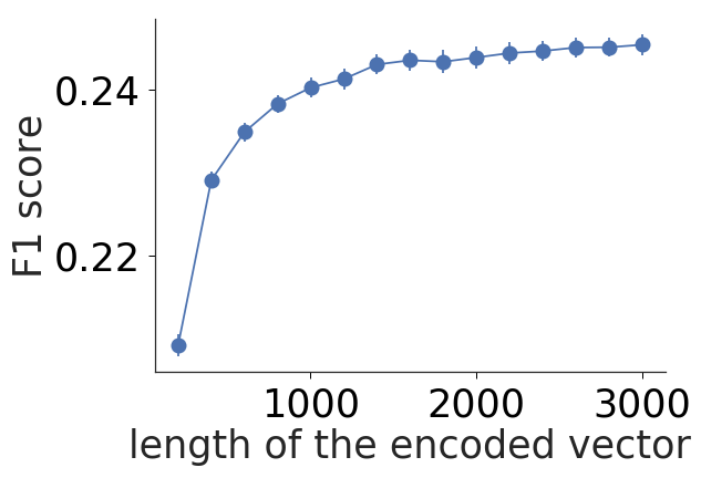
(a) Corel5k

(b) CAL500

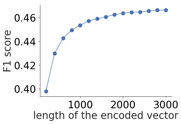
(c) bibtex

(d) enron

(e) medical

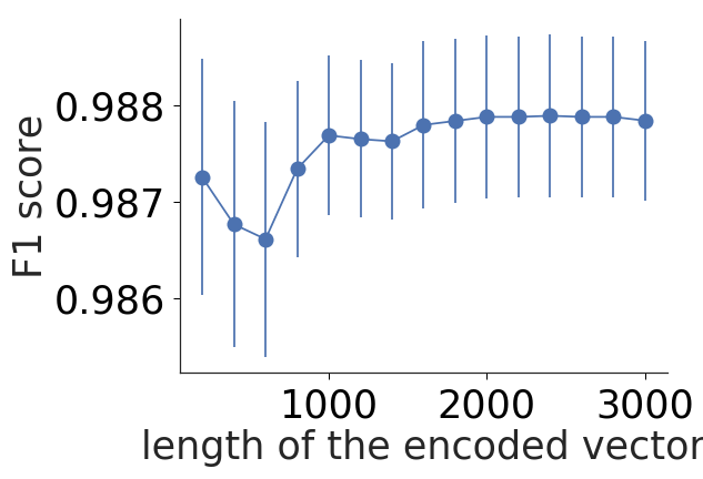
(f) genbase

(g) yeast

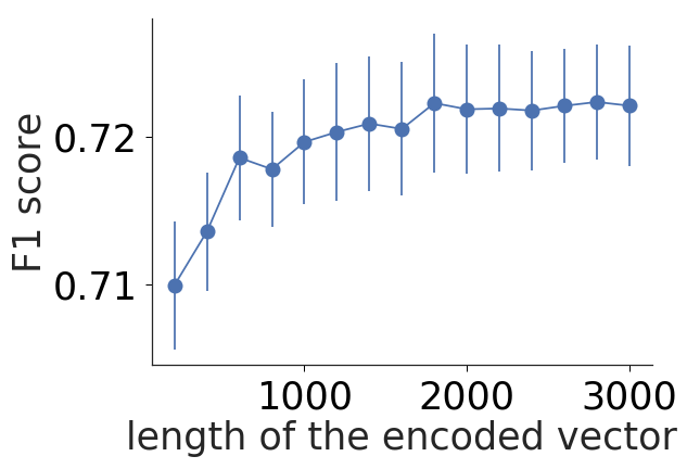
(h) flags

(i) scene

(j) emotions

Figure 2: F1 score $\uparrow$ versus code length for CSRPE

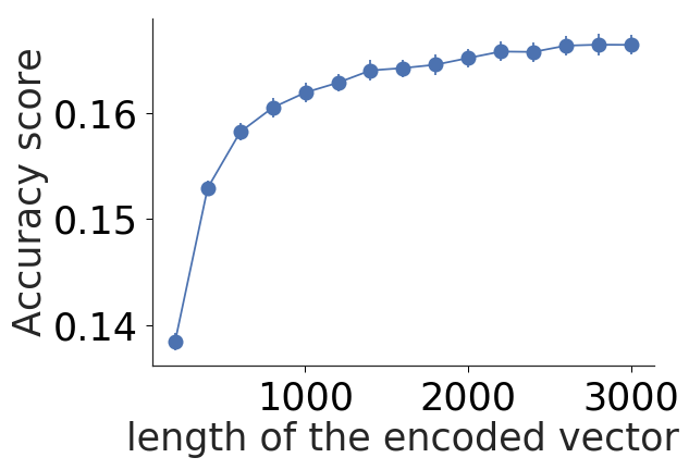
(a) Corel5k

(b) CAL500

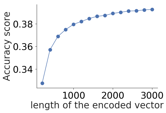
(c) bibtex

(d) enron

(e) medical

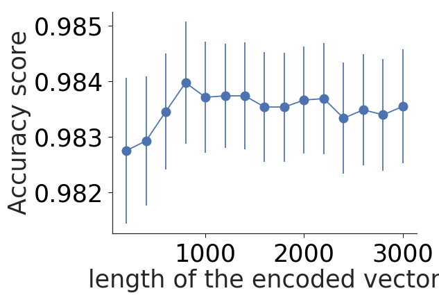
(f) genbase

(g) yeast

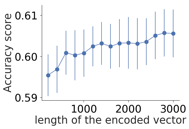
(h) flags

(i) scene

(j) emotions

Figure 3: Accuracy score $\uparrow$ versus code length for CSRPE

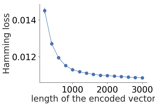
(a) Corel5k

(b) CAL500

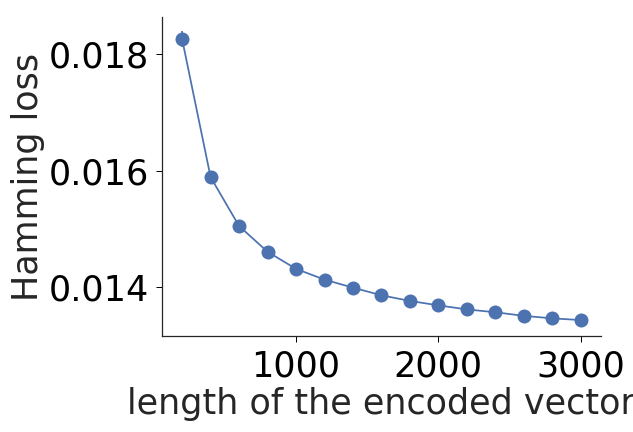
(c) bibtex

(d) enron

(e) medical

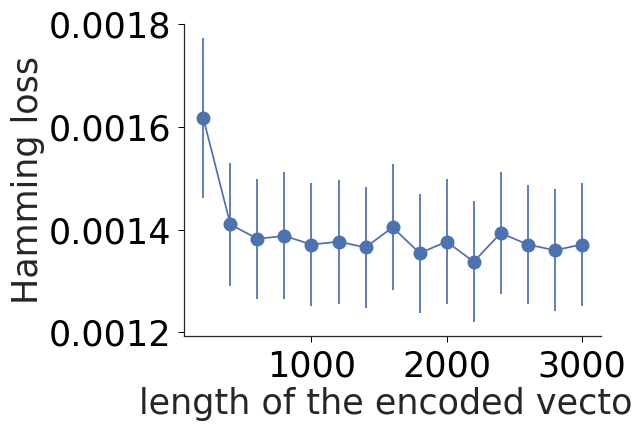
(f) genbase

(g) yeast

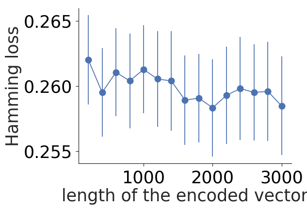
(h) flags

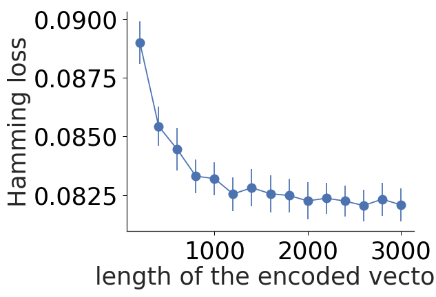
(i) scene

(j) emotions

Figure 4: Hamming loss $\downarrow$ versus code length for CSRPE

(a) Corel5k

(b) CAL500

(c) bibtex

(d) enron

(e) medical

(f) genbase

(g) yeast

(h) flags

(i) scene

(j) emotions

Figure 5: Rank loss $\downarrow$ versus code length for CSRPE

5.2 Influence of the Relevant Set

In Section 3, we claim that a good choice for relevant set $\mathcal{\tilde{Y}}$ is all distinct label vectors in the training dataset. To justify our claim, we demonstrate that the possible downside of this choice, which is the inability to predict all possible label vectors, will not degrade the performance much. In particular, we compare CSRPE with CSRPE-ext, which is CSRPE-ext with a larger relevant set that includes label vectors that appeared in either the training set or the testing set.

Table 2: Experiment results (mean $\pm$ ste) of CSRPE and CSRPE-ext (best in bold)

Dataset	F1 score $\uparrow$		Accuracy score $\uparrow$
	CSRPE	CSRPE-ext	CSRPE	CSRPE-ext
Corel5k	$\mathbf{0.2455\pm 0.0012}$	$0.2492\pm 0.0011$	$0.1664\pm 0.0009$	$\mathbf{0.1674\pm 0.0009}$
bibtex	$0.4663\pm 0.0008$	$\mathbf{0.4695\pm 0.0009}$	$0.3926\pm 0.0011$	$\mathbf{0.3946\pm 0.0010}$
CAL500	$0.4083\pm 0.0017$	$\mathbf{0.4109\pm 0.0013}$	$0.2645\pm 0.0013$	$\mathbf{0.2690\pm 0.0014}$
enron	$0.5911\pm 0.0014$	$\mathbf{0.5921\pm 0.0016}$	$0.4772\pm 0.0016$	$\mathbf{0.4777\pm 0.0017}$
medical	$0.8203\pm 0.0023$	$\mathbf{0.8204\pm 0.0023}$	$\mathbf{0.7939\pm 0.0024}$	$0.7934\pm 0.0022$
genbase	$\mathbf{0.9878\pm 0.0009}$	$0.9876\pm 0.0009$	$\mathbf{0.9836\pm 0.0010}$	$0.9828\pm 0.0012$
yeast	$0.6670\pm 0.0012$	$\mathbf{0.6679\pm 0.0012}$	$\mathbf{0.5653\pm 0.0012}$	$0.5650\pm 0.0012$
flags	$\mathbf{0.7222\pm 0.0041}$	$0.7192\pm 0.0043$	$\mathbf{0.6056\pm 0.0058}$	$0.6028\pm 0.0052$
scene	$0.7860\pm 0.0020$	$\mathbf{0.7913\pm 0.0014}$	$\mathbf{0.7620\pm 0.0020}$	$0.7563\pm 0.0017$
emotions	$\mathbf{1.5912\pm 0.0198}$	$1.5855\pm 0.0175$	$\mathbf{0.5775\pm 0.0037}$	$0.5774\pm 0.0036$

Dataset	Hamming loss $\downarrow$		Rank loss $\downarrow$
	CSRPE	CSRPE-ext	CSRPE	CSRPE-ext
Corel5k	$0.0108\pm 0.0001$	$\mathbf{0.0106\pm 0.0000}$	$490.1698\pm 1.1959$	$\mathbf{485.73\pm 0.88}$
bibtex	$\mathbf{0.0134\pm 0.0000}$	$\mathbf{0.0134\pm 0.0000}$	$104.9449\pm 0.3814$	$\mathbf{102.7833\pm 0.3211}$
CAL500	$0.1651\pm 0.0005$	$\mathbf{0.1638\pm 0.0004}$	$1304.6118\pm 4.5735$	$\mathbf{1303.3491\pm 4.1772}$
enron	$0.0500\pm 0.0003$	$\mathbf{0.0491\pm 0.0002}$	$34.3199\pm 0.1815$	$\mathbf{33.4665\pm 0.2060}$
medical	$0.0100\pm 0.0002$	$\mathbf{0.0098\pm 0.0001}$	$\mathbf{5.3300\pm 0.0676}$	$5.4147\pm 0.0808$
genbase	$0.0014\pm 0.0001$	$\mathbf{0.0013\pm 0.0001}$	$\mathbf{0.3526\pm 0.0304}$	$0.3603\pm 0.0315$
yeast	$\mathbf{0.1891\pm 0.0006}$	$\mathbf{0.1891\pm 0.0006}$	$8.4511\pm 0.0298$	$\mathbf{8.4481\pm 0.0255}$
flags	$0.2585\pm 0.0038$	$\mathbf{0.2580\pm 0.0034}$	$\mathbf{3.0101\pm 0.0470}$	$3.0500\pm 0.0496$
scene	$\mathbf{0.0821\pm 0.0007}$	$0.0822\pm 0.0008$	$0.6793\pm 0.0083$	$\mathbf{0.6453\pm 0.0061}$
emotions	$\mathbf{0.1994\pm 0.0022}$	$0.1996\pm 0.0023$	$\mathbf{0.5911\pm 0.0014}$	$0.5921\pm 0.0016$

The results, which contain the mean and standard error (ste) of the criteria, are listed in Table 2. The results demonstrate that CSRPE-ext is slightly better performing, but the improvement is at best marginal and insignificant. Even in the CAL500 dataset, where all the label vectors in training and testing sets are different, there is only a small performance difference between CSRPE and CSRPE-ext. The result verifies that our choice of $\mathcal{\tilde{Y}}$ as all the distinct label vectors in the training set is sufficiently good.

5.3 Comparison with Other Algorithms

In this experiment, we compare the performance of various MLC and CSMLC algorithms. For the MLC competitors, we include different codes applied within ML-ECC framework. The competing codes include the Hamming on repetition code (HAMR), repetition code (REP), and RAKEL repetition code (RREP) [7]. REP and RREP are equivalent to BR [3] and RAKEL [17], respectively. In addition, CC [4] is added to serve as a baseline competitor together with REP and RREP. For CSMLC algorithms, we compete with PCC [5] and CFT [6].

The results are shown in Table 3 and 4. The results show that CSMLC algorithms generally outperform traditional MLC algorithms. This justifies that it is important to take cost information into account. Among the CSMLC algorithms, CSRPE is superior over all other competitors with respect to F1 and Accuracy score. For Rank loss, PCC performs slightly better, but CSRPE still performs competitively with PCC and CFT. Such result justifies CSRPE as a top performing CSMLC algorithm.

Table 3: Experiment results (mean $\pm$ ste) on different criteria (best in bold)

F1 score $\uparrow$
Dataset	REP (BR)	RREP (RAKEL)	HAMR	CC	PCC	CFT	CSRPE
Corel5k	$.0683\pm.0011$	$.1028\pm.0010$	$.0608\pm.0008$	$.0661\pm.0009$	$.1759\pm.0008$	$.1708\pm.0017$	$\mathbf{.2455\pm.0012}$
CAL500	$.3388\pm.0014$	$.3527\pm.0011$	$.3152\pm.0012$	$.3354\pm.0024$	$.3540\pm.0018$	$.3815\pm.0016$	$\mathbf{.4083\pm.0017}$
bibtex	$.3636\pm.0009$	$.3761\pm.0010$	$.3658\pm.0008$	$.3569\pm.0009$	$.3736\pm.0011$	$.3957\pm.0015$	$\mathbf{.4663\pm.0008}$
enron	$.5441\pm.0026$	$.5336\pm.0025$	$.5459\pm.0023$	$.5492\pm.0022$	$.5508\pm.0014$	$.5530\pm.0013$	$\mathbf{.5911\pm.0014}$
medical	$.7883\pm.0028$	$.7757\pm.0034$	$.7877\pm.0031$	$.7924\pm.0035$	$.8131\pm.0023$	$.7970\pm.0031$	$\mathbf{.8203\pm.0023}$
genbase	$.9897\pm.0012$	$.9893\pm.0014$	$.9896\pm.0012$	$.9896\pm.0012$	$\mathbf{.9911\pm.0007}$	$.9845\pm.0009$	$.9878\pm.0008$
yeast	$.6119\pm.0014$	$.6130\pm.0011$	$.6171\pm.0015$	$.5968\pm.0018$	$.6013\pm.0013$	$.6111\pm.0024$	$\mathbf{.6670\pm.0012}$
flags	$.6954\pm.0045$	$.6965\pm.0044$	$.7005\pm.0044$	$.6973\pm.0048$	$.7075\pm.0038$	$.6725\pm.0055$	$\mathbf{.7222\pm.0041}$
scene	$.5895\pm.0026$	$.5926\pm.0019$	$.6365\pm.0021$	$.6547\pm.0019$	$.7306\pm.0016$	$.6592\pm.0027$	$\mathbf{.7860\pm.0020}$
emotions	$.5968\pm.0038$	$.5773\pm.0047$	$.6100\pm.0035$	$.6205\pm.0035$	$.6384\pm.0033$	$.6015\pm.0043$	$\mathbf{.6655\pm.0035}$
Accuracy score $\uparrow$
Dataset	REP (BR)	RREP (RAKEL)	HAMR	CC	PCC	CFT	CSRPE
Corel5k	$.0471\pm.0007$	$.0696\pm.0006$	$.0408\pm.0009$	$.0471\pm.0007$	$.1135\pm.0005$	$.0790\pm.0019$	$\mathbf{.1664\pm.0009}$
CAL500	$.2097\pm.0010$	$.2179\pm.0008$	$.1925\pm.0007$	$.2085\pm.0018$	$.2209\pm.0012$	$.2425\pm.0015$	$\mathbf{.2645\pm.0013}$
bibtex	$.3063\pm.0009$	$.3103\pm.0009$	$.3094\pm.0008$	$.3031\pm.0010$	$.2940\pm.0010$	$.3235\pm.0011$	$\mathbf{.3926\pm.0011}$
enron	$.4303\pm.0023$	$.4215\pm.0022$	$.4344\pm.0024$	$.4437\pm.0021$	$.4259\pm.0013$	$.4363\pm.0018$	$\mathbf{.4772\pm.0016}$
medical	$.7559\pm.0034$	$.7431\pm.0033$	$.7604\pm.0033$	$.7643\pm.0035$	$.7716\pm.0025$	$.7570\pm.0031$	$\mathbf{.7939\pm.0024}$
genbase	$.9859\pm.0014$	$.9852\pm.0015$	$.9856\pm.0014$	$.9858\pm.0014$	$\mathbf{.9873\pm.0009}$	$.9792\pm.0012$	$.9835\pm.0010$
yeast	$.5047\pm.0014$	$.5065\pm.0012$	$.5120\pm.0015$	$.4954\pm.0021$	$.4872\pm.0017$	$.5027\pm.0019$	$\mathbf{.5653\pm.0012}$
flags	$.5849\pm.0047$	$.5860\pm.0046$	$.5913\pm.0051$	$.5908\pm.0057$	$.5974\pm.0041$	$.5616\pm.0059$	$\mathbf{.6056\pm.0058}$
scene	$.5791\pm.0025$	$.5816\pm.0020$	$.6258\pm.0017$	$.6457\pm.0018$	$.6821\pm.0019$	$.6467\pm.0029$	$\mathbf{.7620\pm.0020}$
emotions	$.5179\pm.0037$	$.4959\pm.0045$	$.5320\pm.0034$	$.5417\pm.0035$	$.5433\pm.0035$	$.5216\pm.0036$	$\mathbf{.5775\pm.0037}$
Hamming loss $\downarrow$
Dataset	REP (BR)	RREP (RAKEL)	HAMR	CC	PCC	CFT	CSRPE
Corel5k	$.0095\pm.0000$	$.0097\pm.0000$	$\mathbf{.0094\pm.0000}$	$.0095\pm.0000$	$.0095\pm.0000$	$.0100\pm.0000$	$.0108\pm.0001$
CAL500	$.1522\pm.0010$	$\mathbf{.1416\pm.0003}$	$.1490\pm.0005$	$.1493\pm.0006$	$.1493\pm.0006$	$.1422\pm.0005$	$.1651\pm.0005$
bibtex	$\mathbf{.0124\pm.0000}$	$.0130\pm.0000$	$.0124\pm.0000$	$.0125\pm.0000$	$.0125\pm.0000$	$.0136\pm.0000$	$.0134\pm.0000$
enron	$.0489\pm.0002$	$.0499\pm.0002$	$.0485\pm.0002$	$.0506\pm.0002$	$.0506\pm.0002$	$\mathbf{.0477\pm.0002}$	$.0500\pm.0003$
medical	$.0104\pm.0002$	$.0107\pm.0001$	$.0102\pm.0002$	$.0103\pm.0002$	$.0105\pm.0001$	$.0111\pm.0002$	$\mathbf{.0100\pm.0002}$
genbase	$.0012\pm.0001$	$.0011\pm.0001$	$\mathbf{.0011\pm.0001}$	$.0011\pm.0001$	$.0012\pm.0001$	$.0016\pm.0001$	$.0014\pm.0001$
yeast	$.1941\pm.0007$	$.1933\pm.0006$	$.1932\pm.0007$	$.2040\pm.0009$	$.2043\pm.0009$	$.2080\pm.0010$	$\mathbf{.1891\pm.0006}$
flags	$.2591\pm.0037$	$.2591\pm.0027$	$.2599\pm.0037$	$.2611\pm.0037$	$.2636\pm.0038$	$.2899\pm.0040$	$\mathbf{.2585\pm.0038}$
scene	$.0914\pm.0004$	$.0970\pm.0005$	$.0848\pm.0005$	$.0919\pm.0007$	$.0924\pm.0007$	$.1031\pm.0009$	$\mathbf{.0821\pm.0007}$
emotions	$.1966\pm.0021$	$.2110\pm.0022$	$\mathbf{.1953\pm.0019}$	$.1959\pm.0018$	$.1958\pm.0020$	$.2207\pm.0020$	$.1994\pm.0022$
Rank loss $\downarrow$
Dataset	REP (BR)	RREP (RAKEL)	HAMR	CC	PCC	CFT	CSRPE
Corel5k	$618.1\pm.6695$	$597.2\pm.6664$	$623.5\pm.6474$	$636.0\pm.5374$	$421.2\pm.6626$	$\mathbf{300.7\pm.7848}$	$490.2\pm 1.1959$
CAL500	$1500.\pm 5.023$	$1477.\pm 4.835$	$1537.\pm 4.488$	$1520.\pm 6.155$	$1179.\pm 4.498$	$\mathbf{1122.\pm 4.470}$	$1305.\pm 4.574$
bibtex	$132.6\pm.2981$	$124.1\pm.2511$	$131.5\pm.2819$	$136.8\pm.2886$	$\mathbf{69.10\pm.2454}$	$112.06\pm.2811$	$104.9\pm.3814$
enron	$43.39\pm.2919$	$44.06\pm.2810$	$43.40\pm.2540$	$43.56\pm.3000$	$27.94\pm.1681$	$\mathbf{27.20\pm.1365}$	$34.32\pm.1815$
medical	$5.454\pm.1184$	$5.733\pm.1088$	$5.601\pm.1232$	$5.469\pm.0997$	$\mathbf{3.058\pm.0603}$	$4.117\pm.0741$	$5.330\pm.0676$
genbase	$.2461\pm.0281$	$.2422\pm.0273$	$.2525\pm.0257$	$.2423\pm.0308$	$\mathbf{.1976\pm.0178}$	$.4686\pm.0310$	$.3863\pm.0341$
yeast	$9.609\pm.0358$	$9.565\pm.0290$	$9.443\pm.0312$	$10.324\pm.0448$	$9.378\pm.0365$	$9.473\pm.0363$	$\mathbf{8.451\pm.0298}$
flags	$3.123\pm.0434$	$3.139\pm.0383$	$3.078\pm.0352$	$3.120\pm.0450$	$3.012\pm.0490$	$3.363\pm.0504$	$\mathbf{3.010\pm.0470}$
scene	$1.136\pm.0066$	$1.149\pm.0055$	$1.031\pm.0046$	$1.098\pm.0080$	$0.726\pm.0060$	$0.892\pm.0069$	$\mathbf{0.679\pm.0083}$
emotions	$1.789\pm.0182$	$1.906\pm.0220$	$1.764\pm.0165$	$1.741\pm.0207$	$\mathbf{1.563\pm.0176}$	$1.834\pm.0281$	$1.591\pm.0198$

Table 4: CSRPE versus others based on $t$-test at 95% confident level (win/tie/loss)

criteria	REP(BR)	RREP(RAKEL)	HAMR	CC	CFT	PCC
f1	9/1/0	9/1/0	9/1/0	9/1/0	9/1/0	9/0/1
acc.	9/0/1	9/1/0	8/2/0	8/2/0	9/1/0	8/1/1
hamming	2/4/4	4/3/3	2/4/4	6/1/3	6/1/3	3/4/3
rank.	7/2/1	9/0/1	7/2/1	7/2/1	6/1/3	2/2/6
total	27/7/6	31/5/4	26/9/5	30/6/4	30/4/6	22/7/11

5.4 Comparison with MLAL Algorithms

In this experiment, we evaluate the performance of CSRPE under the CSMLAL setting. We compare it with several state-of-the-art MLAL algorithms, which includes adaptive active learning (adaptive) [11], maximal loss reduction with maximal confidence (MMC) [10], and random sampling as a baseline algorithm. Their implementations were obtained from libact [18]. We do not include a comparison with binary minimization [9] since MMC and adaptive are reported to outperform it.

(a) CAL500

(b) enron

(c) medical

(d) yeast

(e) scene

(f) emotions

Figure 6: CSMLAL results with F1 score $\uparrow$

(a) CAL500

(b) enron

(c) medical

(d) yeast

(e) scene

(f) emotions

Figure 7: CSMLAL results with Accuracy score $\uparrow$

(a) CAL500

(b) enron

(c) medical

(d) yeast

(e) scene

(f) emotions

Figure 8: CSMLAL results with Hamming loss $\downarrow$

(a) CAL500

(b) enron

(c) medical

(d) yeast

(e) scene

(f) emotions

Figure 9: CSMLAL results with Rank loss $\downarrow$

Figures 6, 7, 8, and 9 show the performance with respect to the number of instances queried. For F1 score and Rank loss, CSRPE performs better than other strategies on four out of six datasets. These results indicate that CSRPE is able to consider the cost information, thus enabling it to outperform other competitors on most of the datasets across different evaluation criteria.

6 Conclusion

In this paper, we propose a novel approach for cost-sensitive multi-label classification (CSMLC), called cost-sensitive reference pair encoding (CSRPE). CSRPE is derived from the one-versus-one algorithm and can embed the cost information into the encoded vectors. Exploiting the redundancy of the encoded vectors, we use random sampling to resolve the training challenge of building so many classifiers. We also design a nearest-neighbor-based decoding procedure and use the relevant set to efficiently make cost-sensitive predictions. Extensive experimental results demonstrate that CSRPE achieves stable convergence respect to the code length and outperforms not only other encoding methods but also state-of-the-art CSMLC algorithms across different cost functions. In addition, we extend CSRPE to a novel multi-label active learning algorithm by designing a cost-sensitive uncertainty measure. Extensive empirical studies show that the proposed active learning algorithm performs better than existing active learning algorithms. The results suggest that CSRPE is a promising cost-sensitive encoding method for CSMLC for either supervised or active learning.

References

- [1] Katakis, I., Tsoumakas, G., Vlahavas, I.: Multilabel text classification for automated tag suggestion. ECML PKDD discovery challenge 75 (2008)
- [2] Liu, Y.: Active learning with support vector machine applied to gene expression data for cancer classification. Journal of Chemical Information and Computer Sciences (2004) 1936–1941
- [3] Tsoumakas, G., Katakis, I., Vlahavas, I.P.: Mining multi-label data. In: Data Mining and Knowledge Discovery Handbook. (2010) 667–685
- [4] Read, J., Pfahringer, B., Holmes, G., Frank, E.: Classifier chains for multi-label classification. Machine learning 85(3) (2011) 333–359
- [5] Dembczynski, K., Cheng, W., Hüllermeier, E.: Bayes optimal multilabel classification via probabilistic classifier chains. In: ICML. (2010)
- [6] Li, C.L., Lin, H.T.: Condensed filter tree for cost-sensitive multi-label classification. In: ICML. (2014)
- [7] Ferng, C.S., Lin, H.T.: Multilabel classification using error-correcting codes of hard or soft bits. IEEE Transactions on Neural Networks and Learning Systems 24(11) (2013) 1888–1900
- [8] Lin, H.T.: Reduction from cost-sensitive multiclass classification to one-versus-one binary classification. In: ACML. (2014)
- [9] Brinker, K.: On active learning in multi-label classification. In: From Data and Information Analysis to Knowledge Engineering. (2006) 206–213
- [10] Yang, B., Sun, J.T., Wang, T., Chen, Z.: Effective multi-label active learning for text classification. In: ICDM. (2009)
- [11] Li, X., Guo, Y.: Active learning with multi-label svm classification. In: IJCAI. (2013)
- [12] Allwein, E.L., Schapire, R.E., Singer, Y.: Reducing multiclass to binary: A unifying approach for margin classifiers. Journal of Machine Learning Research 1 (2001) 113–141
- [13] Liu, T., Moore, A.W., Gray, A.: New algorithms for efficient high-dimensional nonparametric classification. Journal of Machine Learning Research 7 (2006) 1135–1158
- [14] Huang, K.H., Lin, H.T.: Cost-sensitive label embedding for multi-label classification. Machine Learning (2017) 1725–1746
- [15] Settles, B.: Active learning literature survey. University of Wisconsin, Madison (2010)
- [16] Tsoumakas, G., Spyromitros-Xioufis, E., Vilcek, J., Vlahavas, I.: Mulan: A java library for multi-label learning. Journal of Machine Learning Research 12 (2011) 2411–2414
- [17] Tsoumakas, G., Vlahavas, I.P.: Random k-labelsets: An ensemble method for multilabel classification. In: ECML. (2007)
- [18] Yang, Y.Y., Lee, S.C., Chung, Y.A., Wu, T.E., Chen, S.A., Lin, H.T.: libact: Pool-based active learning in python. Technical report, National Taiwan University (October 2017) available as arXiv preprint https://arxiv.org/abs/1710.00379.