Freezing Traveling and Rotating Waves
in Second Order Evolution Equations

Wolf-Jürgen Beyn^,

Denny Otten^,

Department of Mathematics

Bielefeld University

33501 Bielefeld

Germany

Jens Rottmann-Matthes^,

Institut für Analysis

Karlsruhe Institute of Technology

76131 Karlsruhe

Germany

Date: March 8, 2024

Key words. Systems of damped wave equations, traveling waves, rotating waves, freezing method, second order evolution equations, point spectra, essential spectra.

AMS subject classification. 35K57, 35Pxx, 65Mxx (35Q56, 47N40, 65P40).

1. Introduction

The topic of this paper is the numerical computation and stability of waves occurring in nonlinear second order evolution equations with damping terms. Our main object of study is the damped wave equation in one or several space dimensions with a nonlinearity of semilinear type (see (1.1), (1.5) below). In the literature there are many approaches to the numerical solution of the Cauchy problem for such equations by various types of spatial and temporal discretizations. We refer, for example, to the recent papers [10], [14], [1], [19]. Most of the results concern finite time error estimates, and there are a few studies of detecting blow-up solutions or the shape of a developing solitary wave.

In our work we take a different numerical approach which emphasizes the longtime behavior and tries to determine the shape and speed of traveling and rotating waves from a reformulation of the original PDE. More specifically, we transfer the so called freezing method (see [8], [24], [5]) from first order to second order evolution equations, and we investigate its relation to the stability of the waves. Generally speaking, the method tries to separate the solution of a Cauchy problem into the motion of a co-moving frame and of a profile, where the latter is required to vary as little as possible or even become stationary. This is achieved by transforming the original PDE into a partial differential algebraic equation (PDAE). The PDAE involves extra unknowns specifying the frame, and extra constraints (so called phase conditions) enforcing the freezing principle for the profile. This methodology has been successfully applied to a wide range of PDEs which are of first order in time and of hyperbolic, parabolic or of mixed type, cf. [26], [28], [27], [7], [21], [22], [23], [5]. One aim of the theoretical underpinning is to prove that waves which are (asymptotically) stable with asymptotic phase for the PDE, become stable in the classical Lyapunov sense for the PDAE. While this has been rigorously proved for many systems in one space dimension and confirmed numerically in higher space dimensions, the corresponding theory for the multi-dimensional case is still in its early stages, see [2], [4], [3], [18].

In this paper we develop the freezing formulation and perform the spectral calculations in an informal way, for the one-dimensional as well as the multi-dimensional case. Rigorous stability results for the one-dimensional damped wave equation may be found in [13], [12], [6].

Here we consider a nonlinear wave equation of the form

(1.1) $$Mu_{tt}=Au_{xx}+f(u,u_{x},u_{t}),\,x\in\mathbb{R},\,t\geqslant 0,$$

where $u(x,t)\in\mathbb{R}^{m},A,M\in\mathbb{R}^{m,m}$ and $f:\mathbb{R}^{3m}\to\mathbb{R}^{m}$ is sufficiently smooth. In addition, we assume the matrix $M$ to be nonsingular and $M^{-1}A$ to be positive diagonalizable, which will lead to local wellposedness of the Cauchy problem associated with (1.1). Our interest is in traveling waves

$$u_{\star}(x,t)=v_{\star}(x-\mu_{\star}t),\,x\in\mathbb{R},\,t\geqslant 0,$$

with constant limits at $\pm\infty$, i.e.

(1.2) $$\lim_{\xi\to\pm\infty}v_{\star}(\xi)=v_{\pm}\in\mathbb{R}^{m},\;\lim_{\xi\to\pm\infty}v_{\star,\xi}(\xi)=0,\quad f(v_{\pm},0,0)=0.$$

Transforming (1.1) into a co-moving frame via $u(x,t)=v(\xi,t),\xi=x-\mu_{\star}t$ leads to the system

(1.3) $$Mv_{tt}=(A-\mu_{\star}^{2}M)v_{\xi\xi}+2\mu_{\star}Mv_{\xi t}+f(v,v_{\xi},v_{t}-\mu_{\star}v_{\xi}),\,\xi\in\mathbb{R},\,t\geqslant 0.$$

This system has $v_{\star}$ as a steady state,

(1.4) $$0=(A-\mu_{\star}^{2}M)v_{\star,\xi\xi}+f(v_{\star},v_{\star,\xi},-\mu_{\star}v_{\star,\xi}),\,\xi\in\mathbb{R}.$$

In Section 2 we work out the details of the freezing PDAE based on the ansatz $u(x,t)=v(x-\gamma(t),t)$, $x\in\mathbb{R},t\geq 0$ with the additional unknown function $\gamma(t),t\geq 0$. Solving this PDAE numerically will then be demonstated for a special semilinear case, for which damping occurs and for which the nonlinearity is of quintic type with $5$ zeros. We will also discuss in Section 2.2 the spectral properties of the linear operator obtained by linearizing the right-hand side of (1.3) about the profile $v_{\star}$. First, there is the eigenvalue zero due to shift equivariance, and then we analyze the dispersion curves which are part of the operator’s essential spectrum. If there is sufficient damping in the system (depending on the derivative $D_{3}f$), one can expect the whole nonzero spectrum to lie strictly to the left of the imaginary axis. We refer to [6] for a rigorous proof of nonlinear stability in such a situation, both stability of the wave with asymptotic phase for equation (1.3) and Lyapunov stability of the wave and its speed for the freezing equation.

The subsequent section is devoted to study corresponding problems for multi-dimensional wave equations

(1.5) $$Mu_{tt}+Bu_{t}=A\Delta u+f(u),\,x\in\mathbb{R}^{d},\,t\geqslant 0,$$

where the matrices $A,M$ are as above, the damping matrix $B\in\mathbb{R}^{m,m}$ is given and $f:\mathbb{R}^{m}\to\mathbb{R}^{m}$ is again sufficiently smooth. We look for rotating waves of the form

$$u_{\star}(x,t)=v_{\star}(e^{-tS_{\star}}(x-x_{\star})),\,x\in\mathbb{R}^{d},\,t\geqslant 0,$$

where $x_{\star}\in\mathbb{R}^{d}$ denotes the center of rotation, $S_{\star}\in\mathbb{R}^{d,d}$ is a skew-symmetric matrix, and $v_{\star}:\mathbb{R}^{d}\to\mathbb{R}^{m}$ describes the profile. Transforming (1.5) into a co-rotating frame via $u(x,t)=v(e^{-tS_{\star}}(x-x_{\star}),t)$ now leads to the equation

(1.6) $$Mv_{tt}+Bv_{t}= A\triangle v-Mv_{\xi\xi}(S_{\star}\xi)^{2}+2Mv_{\xi t}S_{\star}\xi-Mv_{\xi}S_{\star}^{2}\xi+Bv_{\xi}S_{\star}\xi+f(v),\,\xi\in\mathbb{R}^{d},\,t\geqslant 0,$$

where our notation for derivatives uses multilinear calculus, e.g.

(1.7) $$(v_{\xi\xi}h_{1}h_{2})_{i}=\sum_{j=1}^{d}\sum_{k=1}^{d}v_{i,\xi_{j}\xi_{k}}(h_{1})_{j}(h_{2})_{k},\quad(\triangle v)_{i}=\sum_{j=1}^{d}v_{i,\xi_{j}\xi_{j}}=\sum_{j=1}^{d}v_{i,\xi\xi}(e^{j})^{2}.$$

The profile $v_{\star}$ of the wave is then a steady state solution of (1.6), i.e.

(1.8) $$0=A\triangle v_{\star}-Mv_{\star,\xi\xi}(S_{\star}\xi)^{2}-Mv_{\star,\xi}S_{\star}^{2}\xi+Bv_{\star,\xi}S_{\star}\xi+f(v_{\star}),\,\xi\in\mathbb{R}^{d}.$$

As is known from first oder in time PDEs, there are several eigenvalues of the linearized operator on the imaginary axis caused by the Euclidean symmmetry, see e.g. [15], [16], [11], [2], [17]. The computations become more involved for the wave equation (1.6), but we will show that the eigenvalues on the imaginary axis are the same as in the parabolic case. Further, determining the dispersion relation, and thus curves in the essential spectrum, now amounts to solving a parameterized quadratic eigenvalue problem which in general can only be solved numerically. Finally, we present a numerical example of a rotating wave for the cubic-quintic Ginzburg-Landau equation. The performance of the freezing method will be demonstrated, and we investigate the numerical eigenvalues approximating the point spectrum on (and close to) the imaginary axis as well as the essential spectrum in the left half-plane.

2. Traveling waves in one space dimension

2.1. Freezing traveling waves.

Consider the Cauchy problem associated with (1.1)

(2.1a) $$Mu_{tt}=Au_{xx}+f(u,u_{x},u_{t}), \,x\in\mathbb{R},\,t\geqslant 0,$$

(2.1b) $$u(\cdot,0)=u_{0},\quad u_{t}(\cdot,0)=v_{0}, \,x\in\mathbb{R},\,t=0,$$

for some initial data $u_{0},v_{0}:\mathbb{R}\rightarrow\mathbb{R}^{m}$ and some nonlinearity $f\in C^{3}(\mathbb{R}^{3m},\mathbb{R})$. Introducing new unknowns $\gamma(t)\in\mathbb{R}$ and $v(\xi,t)\in\mathbb{R}^{m}$ via the freezing ansatz for traveling waves

(2.2) $$u(x,t) =v(\xi,t),\quad\xi:=x-\gamma(t),\,x\in\mathbb{R},\,t\geqslant 0,$$

and inserting (2.2) into (2.1a) by taking

(2.3) $$u_{t}=-\gamma_{t}v_{\xi}+v_{t},\quad u_{tt}=-\gamma_{tt}v_{\xi}+\gamma_{t}^{2}v_{\xi\xi}-2\gamma_{t}v_{\xi t}+v_{tt}$$

into account, we obtain the equation

(2.4) $$Mv_{tt}=(A-\gamma_{t}^{2}M)v_{\xi\xi}+2\gamma_{t}Mv_{\xi t}+\gamma_{tt}Mv_{\xi}+f(v,v_{\xi},v_{t}-\gamma_{t}v_{\xi}),\;\xi\in\mathbb{R},\,t\geqslant 0.$$

Now it is convenient to introduce time-dependent functions $\mu_{1}(t)\in\mathbb{R}$ and $\mu_{2}(t)\in\mathbb{R}$ via

$$\mu_{1}(t):=\gamma_{t}(t),\quad\mu_{2}(t):=\mu_{1,t}(t)=\gamma_{tt}(t)$$

which allows us to transfer (2.4) into a coupled PDE/ODE-system

(2.5a) $$Mv_{tt}=(A-\mu_{1}^{2}M)v_{\xi\xi}+2\mu_{1}Mv_{\xi t}+\mu_{2}Mv_{\xi}+f(v,v_{\xi},v_{t}-\mu_{1}v_{\xi}), \xi\in\mathbb{R},\,t\geqslant 0,$$

(2.5b) $$\mu_{1,t}=\mu_{2}, t\geqslant 0,$$

(2.5c) $$\gamma_{t}=\mu_{1}, t\geqslant 0.$$

The quantity $\gamma(t)$ denotes the position, $\mu_{1}(t)$ the velocity and $\mu_{2}(t)$ the acceleration of the profile $v(\xi,t)$ at time $t$. We next specify initial data for the system (2.5) as follows,

(2.6) $$v(\cdot,0)=u_{0},\quad v_{t}(\cdot,0)=v_{0}+\mu_{1}^{0}u_{0,\xi},\quad\mu_{1}(0)=\mu_{1}^{0},\quad\gamma(0)=0$$

Note that if we require $\gamma(0)=0$ and $\mu_{1}(0)=\mu_{1}^{0}$, then the first equation in (2.6) follows from (2.2) and (2.1b), while the second equation in (2.6) follows from (2.3), (2.1b) and (2.5c). Suitable values for $\mu_{1}^{0}$ depend on the choice of phase condition to be discussed next.

We compensate the extra variable $\mu_{2}$ in the system (2.5) by imposing an additional scalar algebraic constraint, also known as a phase condition, of the general form

(2.7) $$\psi(v,v_{t},\mu_{1},\mu_{2})=0,\;t\geqslant 0.$$

Two possible choices are the fixed phase condition $\psi_{\mathrm{fix}}$ and the orthogonal phase condition $\psi_{\mathrm{orth}}$ given by

(2.8) $$\psi_{\mathrm{fix}}(v)=\langle v-\hat{v},\hat{v}_{\xi}\rangle_{L^{2}},\;t\geqslant 0,$$

$$\psi_{\mathrm{orth}}(v_{t})=\langle v_{t},v_{\xi}\rangle_{L^{2}},\;t\geqslant 0.$$

These two types and their derivation are discussed in [6]. The function $\hat{v}:\mathbb{R}\rightarrow\mathbb{R}^{m}$ denotes a time-independent and sufficiently smooth template (or reference) function, e.g. $\hat{v}=u_{0}$. Suitable values for $\mu_{1}(0)=\mu_{1}^{0}$ can be derived from requiring consistent initial values for the PDAE. For example, consider (2.8) and take the time derivative at $t=0$. Together with (2.6) this leads to $0=\langle v_{t}(\cdot,0),\hat{v}_{\xi}\rangle_{L^{2}}=\langle v_{0},\hat{v}_{\xi}\rangle_{L^{2}}+\mu_{1}^{0}\langle u_{0,\xi},\hat{v}_{\xi}\rangle_{L^{2}}$. If $\langle u_{0,\xi},\hat{v}_{\xi}\rangle_{L^{2}}\neq 0$ this determines a unique value for $\mu_{1}^{0}$.

Let us summarize the set of equations obtained by the freezing method of the original Cauchy problem (2.1). Combining the differential equations (2.5), the initial data (2.6) and the phase condition (2.7), we arrive at the following partial differential algebraic evolution equation (short: PDAE) to be solved numerically:

(2.9a) $$\begin{aligned} Mv_{tt}&=(A-\mu_{1}^{2}M)v_{\xi\xi}+2\mu_{1}Mv_{\xi,t}+\mu_{2}Mv_{\xi}+f(v,v_{\xi},v_{t}-\mu_{1}v_{\xi}),\\ \mu_{1,t}&=\mu_{2},\quad\gamma_{t}=\mu_{1},\end{aligned} t\geqslant 0,$$

(2.9b) $$0=\psi(v,v_{t},\mu_{1},\mu_{2}), t\geqslant 0,$$

(2.9c) $$\begin{aligned} v(\cdot,0)&=u_{0},\quad v_{t}(\cdot,0)=v_{0}+\mu_{1}^{0}u_{0,\xi},\quad\mu_{1}(0)=\mu_{1}^{0},\quad\gamma(0)=0.\end{aligned}$$

The system (2.9) depends on the choice of phase condition $\psi$ and is to be solved for $(v,\mu_{1},\mu_{2},\gamma)$ with given initial data $(u_{0},v_{0},\mu_{1}^{0})$. It consists of a PDE for $v$ that is coupled to two ODEs for $\mu_{1}$ and $\gamma$ (2.9a) and an algebraic constraint (2.9b) which closes the system. A consistent initial value $\mu_{1}^{0}$ for $\mu_{1}$ is computed from the phase condition and the initial data. Further initialization of the algebraic variable $\mu_{2}$ is usually not needed for a PDAE-solver but can be provided if necessary (see [6]).

The ODE for $\gamma$ is called the reconstruction equation in [24]. It decouples from the other equations in (2.9) and can be solved in a postprocessing step. The ODE for $\mu_{1}$ is the new feature of the PDAE for second order systems when compared to the first order parabolic and hyperbolic equations in [8, 20, 5].

Finally, note that $(v,\mu_{1},\mu_{2})=(v_{\star},\mu_{\star},0)$ satisfies

$$0 =(A-\mu_{\star}^{2}M)v_{\star,\xi\xi}+\mu_{\star}Mv_{\star,\xi}+f(v_{\star},v_{\star,\xi},-\mu_{\star}v_{\star,\xi}),\;\xi\in\mathbb{R},$$

$$0 =\mu_{2},$$

$$0 =\psi(v_{\star},0,\mu_{\star},0),$$

and hence is a stationary solution of (2.9a),(2.9b). Here we assume that $v_{\star},\mu_{\star}$ have been selected to satisfy the phase condition. Obviously, in this case we have $\gamma(t)=\mu_{\star}t$. For a stable traveling wave we expect that solutions $(v,\mu_{1},\mu_{2},\gamma)$ of (2.9) show the limiting behavior

$$v(t)\rightarrow v_{\star},\quad\mu_{1}(t)\rightarrow\mu_{\star},\quad\mu_{2}(t)\rightarrow 0\quad\text{as}\quad t\to\infty,$$

provided the initial data are close to their limiting values.

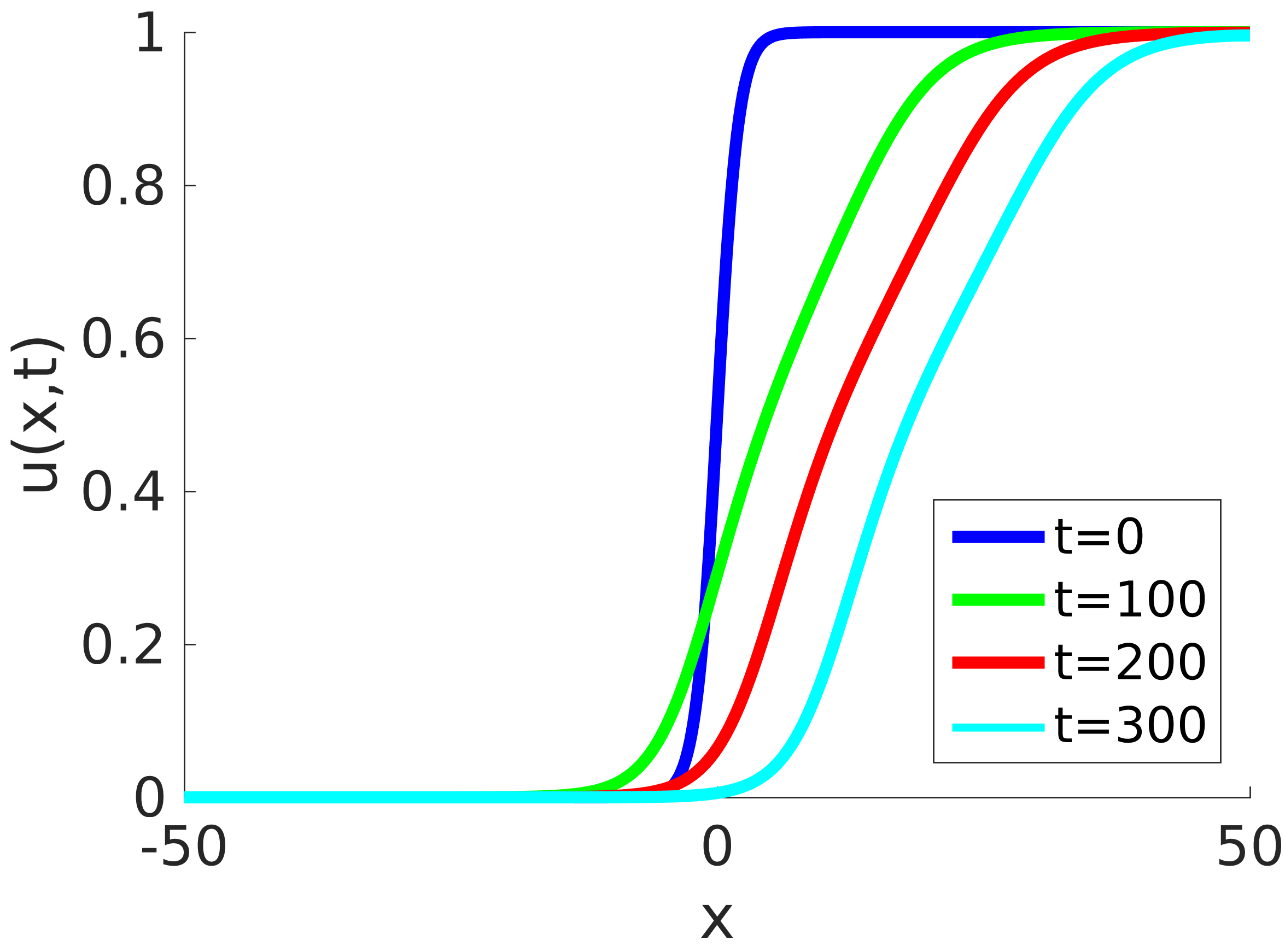
Example 2.1 (Freezing quintic Nagumo wave equation).

Consider the quintic Nagumo wave equation,

(2.10) $$\varepsilon u_{tt}=Au_{xx}+f(u,u_{x},u_{t}),\;x\in\mathbb{R},\,t\geqslant 0,$$

with $u=u(x,t)\in\mathbb{R}$, $\varepsilon>0$, $0<\alpha_{1}<\alpha_{2}<\alpha_{3}<1$, and the nonlinear term

(2.11) $$f:\mathbb{R}^{3}\rightarrow\mathbb{R},\quad f(u,u_{x},u_{t})=-u_{t}+u(1-u)\prod_{j=1}^{3}(u-\alpha_{j}).$$

Figure 2.1. Traveling front of quintic Nagumo wave equation (2.10) at different time instances (a) and its time evolution (b) for parameters from (2.12).

For the parameter values

(2.12) $$M=\varepsilon=\frac{1}{2},\quad A=1,\quad\alpha_{1}=\frac{2}{5},\quad\alpha_{2}=\frac{1}{2},\quad\alpha_{3}=\frac{17}{20},$$

equation (2.10) admits a traveling front solution connecting the asymptotic states $v_{-}=0$ and $v_{+}=1$.

Figure 2.1 shows a numerical simulation of the solution $u$ of (2.10) on the spatial domain $(-50,50)$ with homogeneous Neumann boundary conditions, with initial data

(2.13) $$u_{0}(x)=\tfrac{1}{2}\left(1+\tanh\left(\tfrac{x}{2}\right)\right),\quad v_{0}(x)=0$$

and parameters taken from (2.12). For the space discretization we use continuous piecewise linear finite elements with spatial stepsize $\triangle x=0.1$. For the time discretization we use the BDF method of order $2$ with absolute tolerance $\mathrm{atol}=10^{-3}$, relative tolerance $\mathrm{rtol}=10^{-2}$, temporal stepsize $\triangle t=0.2$ and final time $T=800$. Computations are performed with the help of the software COMSOL 5.2.

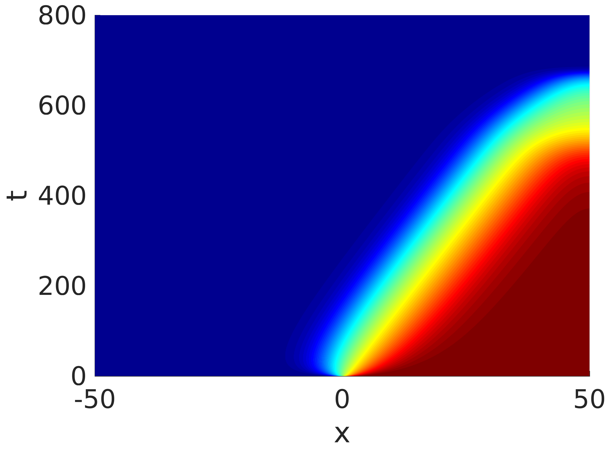
Let us now consider the frozen quintic Nagumo wave equation resulting from (2.9)

(2.14a) $$\begin{aligned} \varepsilon v_{tt}+v_{t}&=(1-\mu_{1}^{2}\varepsilon)v_{\xi\xi}+2\mu_{1}\varepsilon v_{\xi,t}+(\mu_{2}\varepsilon+\mu_{1})v_{\xi}+\tilde{f}(v),\\ \mu_{1,t}&=\mu_{2},\quad\gamma_{t}=\mu_{1},\end{aligned} t\geqslant 0,$$

(2.14b) $$0=\bigl{\langle}v_{t}(\cdot,t),\hat{v}_{\xi}\bigr{\rangle}_{L^{2}(\mathbb{R},\mathbb{R})}, t\geqslant 0,$$

(2.14c) $$\begin{aligned} v(\cdot,0)&=u_{0},\quad v_{t}(\cdot,0)=v_{0}+\mu_{1}^{0}u_{0,\xi},\quad\mu_{1}(0)=\mu_{1}^{0},\quad\gamma(0)=0.\end{aligned}$$

Figure 2.2. Solution of the frozen quintic Nagumo wave equation (2.14): approximation of profile $v(x,1000)$ (a) and time evolutions of velocity $\mu_{1}$ and acceleration $\mu_{2}$ (b) and of the profile $v$ (c) for parameters from (2.12).

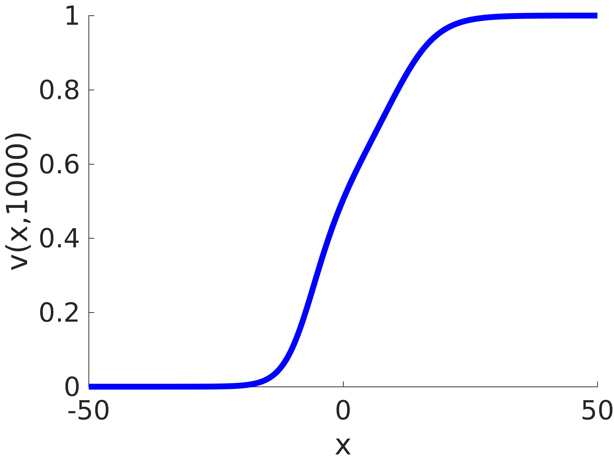
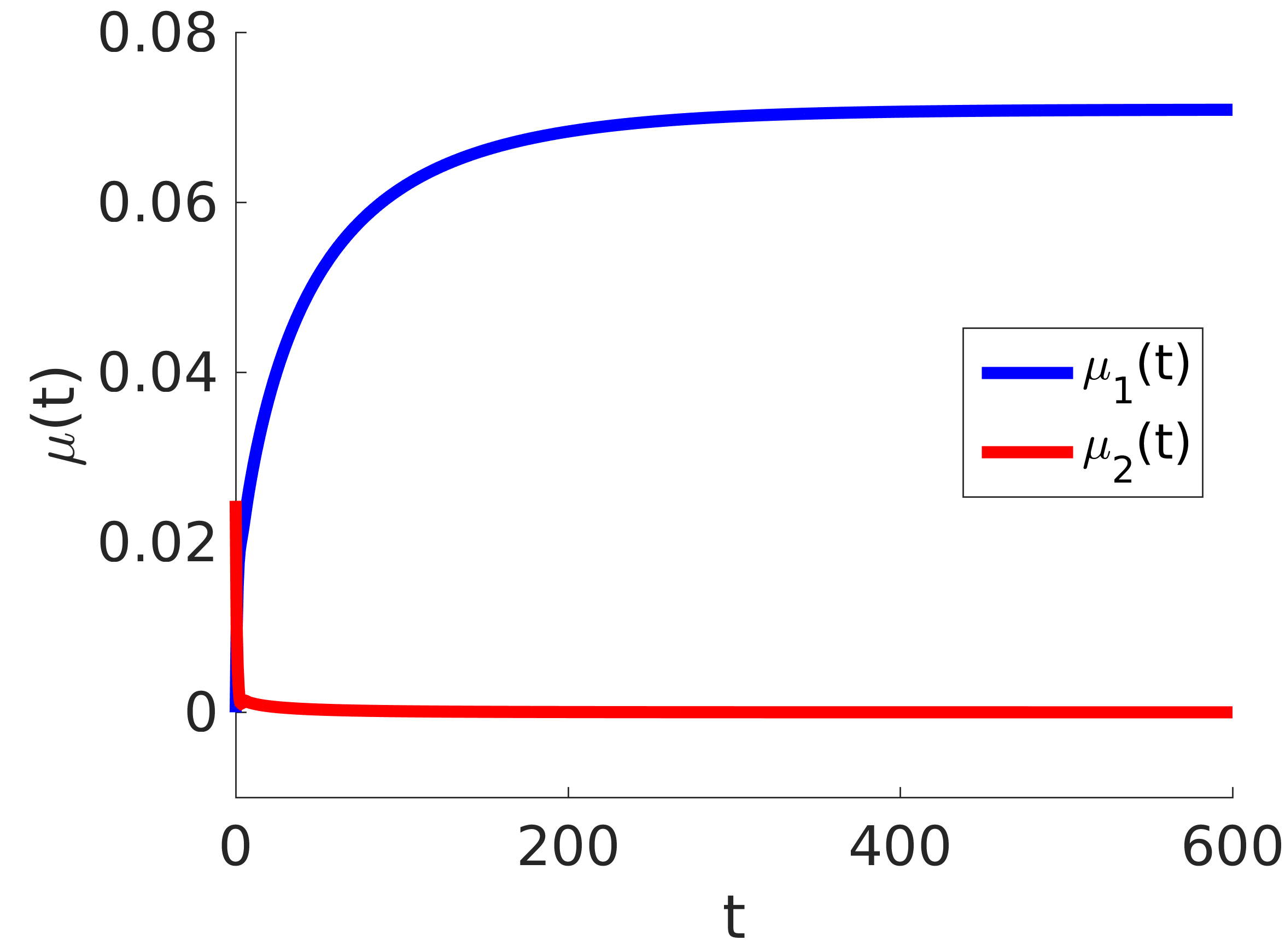
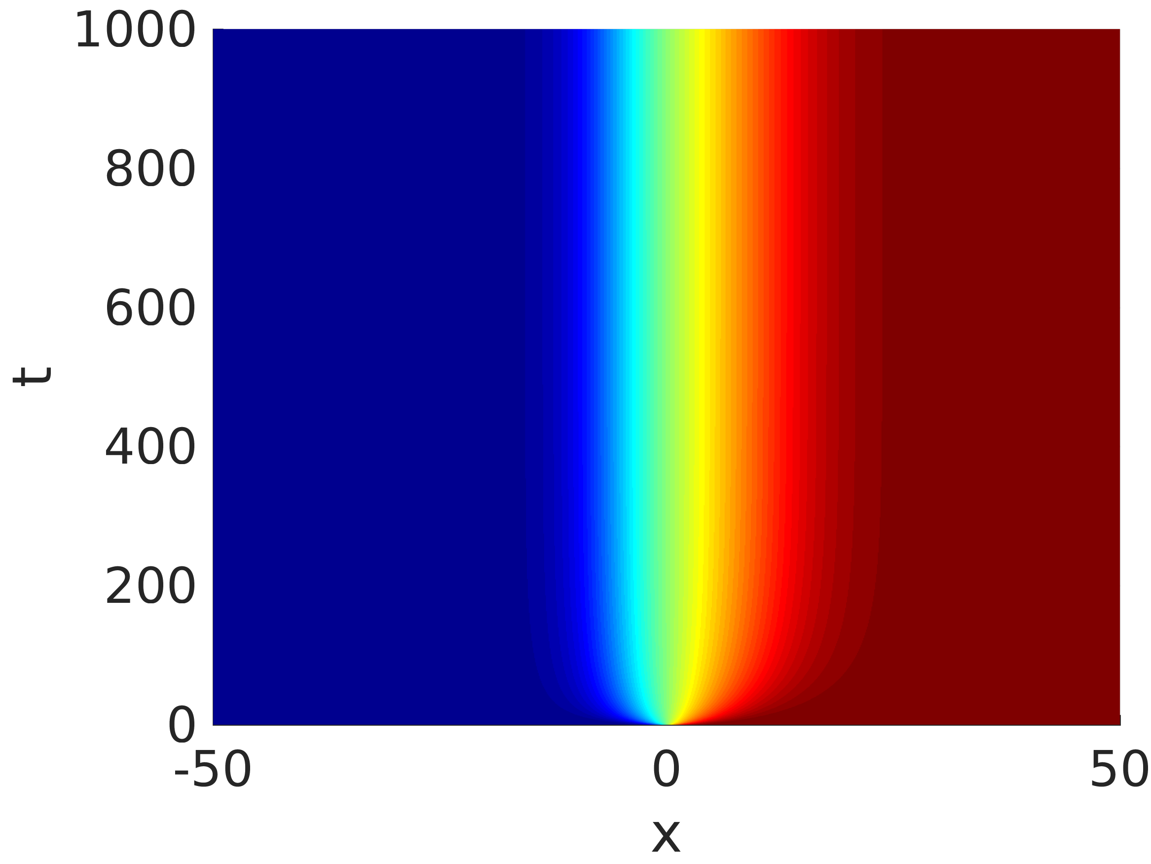
Figure 2.2 shows the solution $(v,\mu_{1},\mu_{2},\gamma)$ of (2.14) on the spatial domain $(-50,50)$ with homogeneous Neumann boundary conditions, initial data $u_{0}$, $v_{0}$ from (2.13), and reference function $\hat{v}=u_{0}$. For the computation we used the fixed phase condition $\psi_{\mathrm{fix}}(v)$ from (2.8) with consistent intial data $\mu_{1}^{0}=0$, see above. The spatial discretization data are taken as in the nonfrozen case. For the time discretization we used the BDF method of order $2$ with absolute tolerance $\mathrm{atol}=10^{-3}$, relative tolerance $\mathrm{rtol}=10^{-2}$, temporal stepsize $\triangle t=0.6$ and final time $T=3000$. The diagrams show that after a very short transition phase the profile becomes stationary, the acceleration $\mu_{2}$ converges to zero, and the speed $\mu_{1}$ approaches an asymptotic value $\mu_{\star}^{\mathrm{num}}=0.0709$.

2.2. Spectra of traveling waves.

Consider the linearized equation

(2.15) $$Mv_{tt}-(A-\mu_{\star}^{2}M)v_{\xi\xi}-2\mu_{\star}Mv_{\xi t}-(D_{2}f_{\star}-\mu_{\star}D_{3}f_{\star})v_{\xi}-D_{3}f_{\star}v_{t}-D_{1}f_{\star}v=0$$

which is obtained from the co-moving frame (1.3) linearized at the profile $v_{\star}$. In (2.15) we use the short form $D_{j}f_{\star}=D_{j}f(v_{\star},v_{\star,\xi},-\mu_{\star}v_{\star,\xi})$. Looking for solutions of the form $v(\xi,t)=e^{\lambda t}w(\xi)$ to (2.15) yields the quadratic eigenvalue problem

(2.16) $$\mathcal{P}(\lambda)w=\left(\lambda^{2}P_{2}+\lambda P_{1}+P_{0}\right)w=0,\,\xi\in\mathbb{R}$$

with differential operators $P_{j}$ defined by

$$P_{2}=M,\quad P_{1}=-2\mu_{\star}M\partial_{\xi}-D_{3}f_{\star},\quad P_{0}=-(A-\mu_{\star}^{2}M)\partial^{2}_{\xi}-(D_{2}f_{\star}-\mu_{\star}D_{3}f_{\star})\partial_{\xi}-D_{1}f_{\star}.$$

We are interested in solutions $(\lambda,w)$ of (2.16) which are candidates for eigenvalues $\lambda\in\mathbb{C}$ and eigenfunctions $w:\mathbb{R}\to\mathbb{C}^{m}$ in suitable function spaces. In fact, it is usually imposssible to determine the spectrum $\sigma(\mathcal{P})$ analytically, but one is able to analyze certain subsets. Let us first calculate the symmetry set $\sigma_{\mathrm{sym}}(\mathcal{P})$, which belongs to the point spectrum $\sigma_{\mathrm{pt}}(\mathcal{P})$ and is affected by the underlying group symmetries. Then, we calculate the dispersion set $\sigma_{\mathrm{disp}}(\mathcal{P})$, which belongs to the essential spectrum $\sigma_{\mathrm{ess}}(\mathcal{P})$ and is affected by the far-field behavior of the wave. Let us first derive the symmetry set of $\mathcal{P}$. This is a simple task for traveling waves but becomes more involved when analyzing the symmetry set for rotating waves (see Section 3.2.2).

Point Spectrum and symmetry set.

Applying $\partial_{\xi}$ to the traveling wave equation (1.4) yields $P_{0}v_{\star,\xi}=0$ which proves the following result.

Proposition 2.2 (Point spectrum of traveling waves).

Let $f\in C^{1}(\mathbb{R}^{3m},\mathbb{R}^{m})$ and let $v_{\star}\in C^{3}(\mathbb{R},\mathbb{R}^{m})$ be a nontrivial classical solution of (1.4) for some $\mu_{\star}\in\mathbb{R}$. Then, $w=v_{\star,\xi}$ and $\lambda=0$ is a classical solution of the eigenvalue problem (2.16). In particular, the symmetry set

$$\sigma_{\mathrm{sym}}(\mathcal{P})=\{0\}$$

belongs to the point spectrum $\sigma_{\mathrm{pt}}(\mathcal{P})$ of $\mathcal{P}$.

Of course, a rigorous statement of this kind requires to specify the function spaces involved, e.g. $L^{2}(\mathbb{R},\mathbb{R}^{m})$ or $H^{1}(\mathbb{R},\mathbb{R}^{m})$, see [13], [12], [6].

Essential Spectrum and dispersion set.

1. The far-field operator. It is a well known fact that the essential spectrum is affected by the limiting equation obtained from (2.16) as $\xi\to\pm\infty$. Therefore, we let formally $\xi\to\pm\infty$ in (2.16) and obtain

   (2.17) $$\left(\lambda^{2}P_{2}+\lambda P_{1}^{\pm}+P_{0}^{\pm}\right)w=0,\;\xi\in\mathbb{R}.$$

   with the constant coefficient operators

   $$P_{2}=M,\quad P_{1}^{\pm}=-2\mu_{\star}M\partial_{\xi}-D_{3}f_{\pm},\quad P_{0}^{\pm}=-(A-\mu_{\star}^{2}M)\partial^{2}_{\xi}-(D_{2}f_{\pm}-\mu_{\star}D_{3}f_{\pm})\partial_{\xi}-D_{1}f_{\pm},$$

   where $v_{\pm}$ are from (1.2) and $D_{j}f_{\pm}=D_{j}f(v_{\pm},0,0)$. We may then write equation (2.16) as

   $$\left(\lambda^{2}P_{2}+\lambda(P_{1}^{\pm}+Q_{1}^{\pm}(\xi))+(P_{0}^{\pm}+Q_{2}^{\pm}(\xi)\partial_{\xi}+Q_{3}^{\pm}(\xi))\right)w=0,\;\xi\in\mathbb{R}$$

   with the perturbation operators defined by

   $$Q_{1}^{\pm}(\xi)=D_{3}f_{\pm}-D_{3}f_{\star},\;\;Q_{2}^{\pm}(\xi)=D_{2}f_{\pm}-D_{2}f_{\star}+\mu_{\star}(D_{3}f_{\star}-D_{3}f_{\pm}),\;\;Q_{3}^{\pm}(\xi)=D_{1}f_{\pm}-D_{1}f_{\star},$$

   Note that $v_{\star}(\xi)\to v_{\pm}$ implies $Q_{j}^{\pm}(\xi)\to 0$ as $\xi\to\pm\infty$ for $j=1,2,3$.

2. Spatial Fourier transform. For $\omega\in\mathbb{R}$, $z\in\mathbb{C}^{m}$, $|z|=1$ we apply the spatial Fourier transform $w(\xi)=e^{i\omega\xi}z$ to equation (2.17) which leads to the $m$-dimensional quadratic eigenvalue problem

   (2.18) $$\left(\lambda^{2}A_{2}+\lambda A_{1}^{\pm}(\omega)+A_{0}^{\pm}(\omega)\right)z=0$$

   with matrices $A_{2}\in\mathbb{R}^{m,m}$ and $A_{1}^{\pm}(\omega),A_{0}^{\pm}(\omega)\in\mathbb{C}^{m,m}$ given by

   (2.19) $$A_{2}=M,\;A_{1}^{\pm}(\omega)=-2i\omega\mu_{\star}M-D_{3}f_{\pm},\;A_{0}^{\pm}(\omega)=\omega^{2}(A-\mu_{\star}^{2}M)-i\omega(D_{2}f_{\pm}-\mu_{\star}D_{3}f_{\pm})-D_{1}f_{\pm}.$$

3. Dispersion relation and dispersion set. The dispersion relation for traveling waves of second order evolution equations states the following: Every $\lambda\in\mathbb{C}$ satisfying

   (2.20) $$\det\left(\lambda^{2}A_{2}+\lambda A_{1}^{\pm}(\omega)+A_{0}^{\pm}(\omega)\right)=0$$

   for some $\omega\in\mathbb{R}$ belongs to the essential spectrum of $\mathcal{P}$, i.e. $\lambda\in\sigma_{\mathrm{ess}}(\mathcal{P})$. Solving (2.20) is equivalent to finding all zeros of a polynomial of degree $2m$. Note that the limiting case $M=0$ in (2.20) leads to the dispersion relation for traveling waves of first order evolution equations, which is well-known in the literature, see [25].

Proposition 2.3 (Essential spectrum of traveling waves).

Let $f\in C^{1}(\mathbb{R}^{3m},\mathbb{R}^{m})$ with $f(v_{\pm},0,0)=0$ for some $v_{\pm}\in\mathbb{R}^{m}$. Let $v_{\star}\in C^{2}(\mathbb{R},\mathbb{R}^{m})$, $\mu_{\star}\in\mathbb{R}$ be a nontrivial classical solution of (1.4) satisfying $v_{\star}(\xi)\to v_{\pm}$ as $\xi\to\pm\infty$. Then, the dispersion set

$$\sigma_{\mathrm{disp}}(\mathcal{P})=\{\lambda\in\mathbb{C}:\text{$\lambda$ satisfies \eqref{equ:2.17} for some $\omega\in\mathbb{R}$, and $+$ or $-$}\}$$

belongs to the essential spectrum $\sigma_{\mathrm{ess}}(\mathcal{P})$ of $\mathcal{P}$.

Example 2.4 (Spectrum of quintic Nagumo wave equation).

As shown in Example 2.1 the quintic Nagumo wave equation (2.10) with coefficients and parameters (2.12) has a traveling front solution $u_{\star}(x,t)=v_{\star}(x-\mu_{\star}t)$ with velocity $\mu_{\star}\approx 0.0709$, whose profile $v_{\star}$ connects the asymptotic states $v_{-}=0$ and $v_{+}=1$ according to (1.2).
We solve numerically the eigenvalue problem for the quintic Nagumo wave equation

(2.21) $$\left(\lambda^{2}\varepsilon+\lambda\left(-2\mu_{\star}\varepsilon\partial_{\xi}-D_{3}f_{\star}\right)+\left(-(1-\mu_{\star}^{2}\varepsilon)\partial^{2}_{\xi}-(D_{2}f_{\star}-\mu_{\star}D_{3}f_{\star})\partial_{\xi}-D_{1}f_{\star}\right)\right)w=0.$$

Both approximations of the profile $v_{\star}$ and the velocity $\mu_{\star}$ in (2.21) are chosen from the solution of (2.14) at time $t=3000$ in Example 2.1. Due to Proposition 2.2 we expect $\lambda=0$ to be an isolated eigenvalue belonging to the point spectrum. Let us next discuss the dispersion set from Proposition 2.3. The quintic Nagumo nonlinearity (2.11) satisfies

$$f_{\pm}=0,\quad D_{3}f_{\pm}=-1,\quad D_{2}f_{\pm}=0,\quad D_{1}f_{-}=-\alpha_{1}\alpha_{2}\alpha_{3},\quad D_{1}f_{+}=-\prod_{j=1}^{3}(1-\alpha_{j}).$$

The matrices $A_{2}$, $A_{1}^{\pm}(\omega)$, $A_{0}^{\pm}(\omega)$ from (2.19) of the quadratic problem (2.18) are given by

$$A_{2}=\varepsilon,\quad A_{1}^{\pm}(\omega)=-2i\omega\mu_{\star}\varepsilon+1,\quad A_{0}^{\pm}(\omega)=\omega^{2}(1-\mu_{\star}^{2}\varepsilon)-i\omega\mu_{\star}-D_{1}f_{\pm}.$$

The dispersion relation (2.20) for the quintic Nagumo front states that every $\lambda\in\mathbb{C}$ satisfying

(2.22) $$\lambda^{2}\varepsilon+\lambda(-2i\omega\mu_{\star}\varepsilon+1)+(\omega^{2}(1-\mu_{\star}^{2}\varepsilon)-i\omega\mu_{\star}-D_{1}f_{\pm})=0$$

for some $\omega\in\mathbb{R}$, and for $+$ or $-$, belongs to $\sigma_{\mathrm{ess}}(\mathcal{P})$. We introduce a new unknown $\tilde{\lambda}\in\mathbb{C}$ via $\lambda=\tilde{\lambda}+i\omega\mu_{\star}$ and solve the transformed equation

$$\tilde{\lambda}^{2}+\frac{1}{\varepsilon}\tilde{\lambda}+\frac{1}{\varepsilon}(\omega^{2}-D_{1}f_{\pm})=0.$$

obtained from (2.22). Thus, the quadratic eigenvalue problem (2.22) has the solutions

$$\lambda=-\frac{1}{2\varepsilon}+i\omega\mu_{\star}\pm\frac{1}{2\varepsilon}\sqrt{1-4\varepsilon(\omega^{2}-D_{1}f_{\pm})},\,\omega\in\mathbb{R}.$$

These solutions lie on the line $\mathrm{Re}=-\frac{1}{2\varepsilon}$ and on two ellipses if $-4D_{1}f_{\pm}\varepsilon<1$ (cf. Figure 2.3(a)).

Figure 2.3. Spectrum of the quintic Nagumo wave equation for parameters (2.12) (a) and the numerical spectrum on the spatial domain $[-R,R]$ for $R=50$ (b) and $R=400$ (c) both for spatial stepsize $\triangle x=0.1$.

Figure 2.4. Eigenfunctions of the quintic Nagumo wave equation for parameters (2.12) belonging to the isolated eigenvalues $\lambda_{1}\approx 0$ (a), $\lambda_{2}\approx-0.011274$ (b), and a zoom into the spectrum from Fig.2.3(c) in (c).

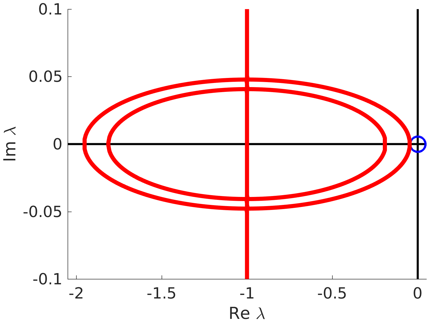
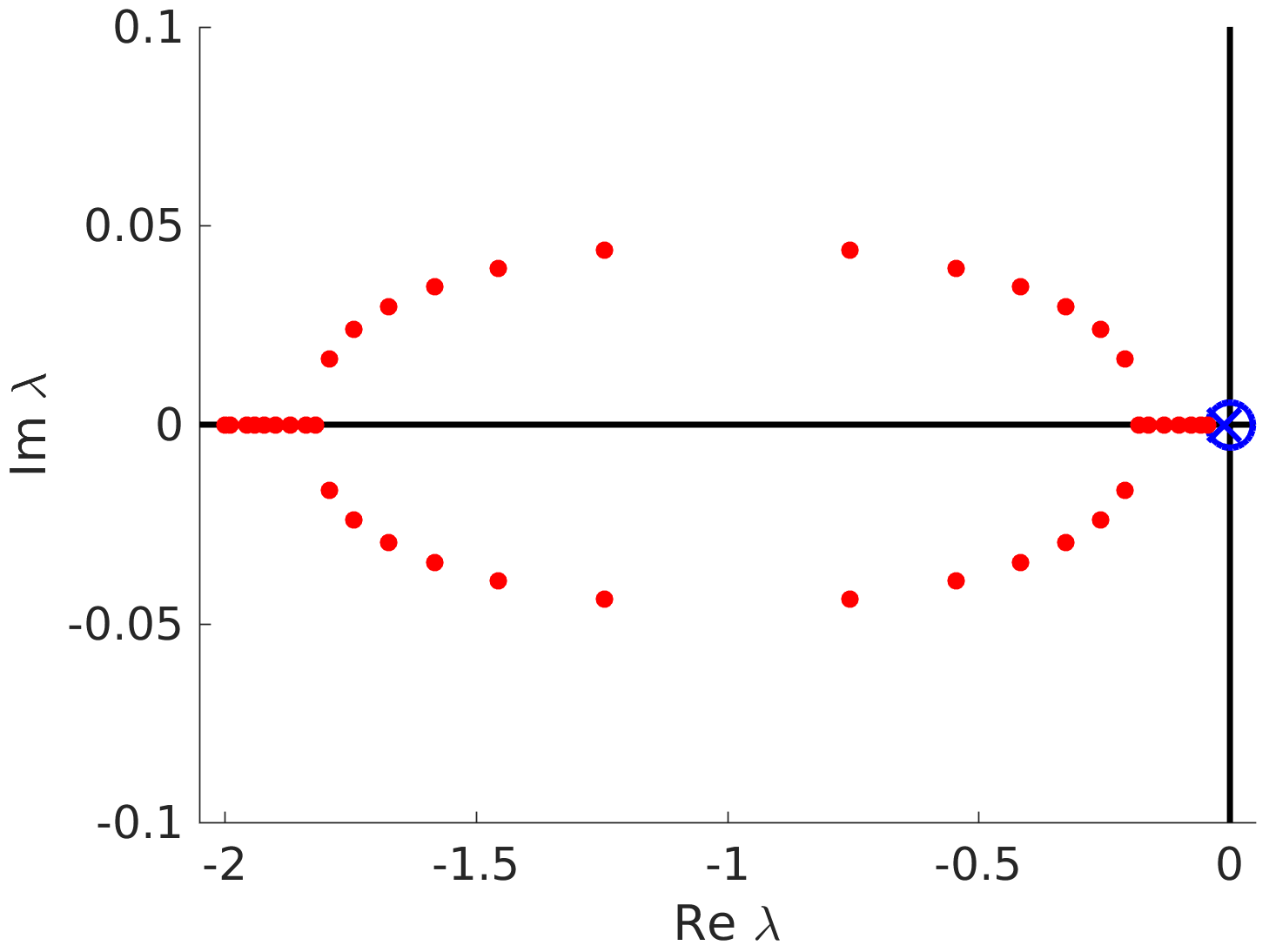
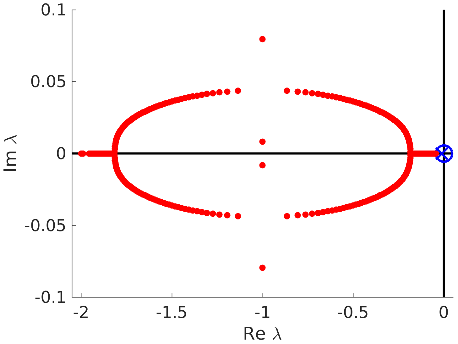
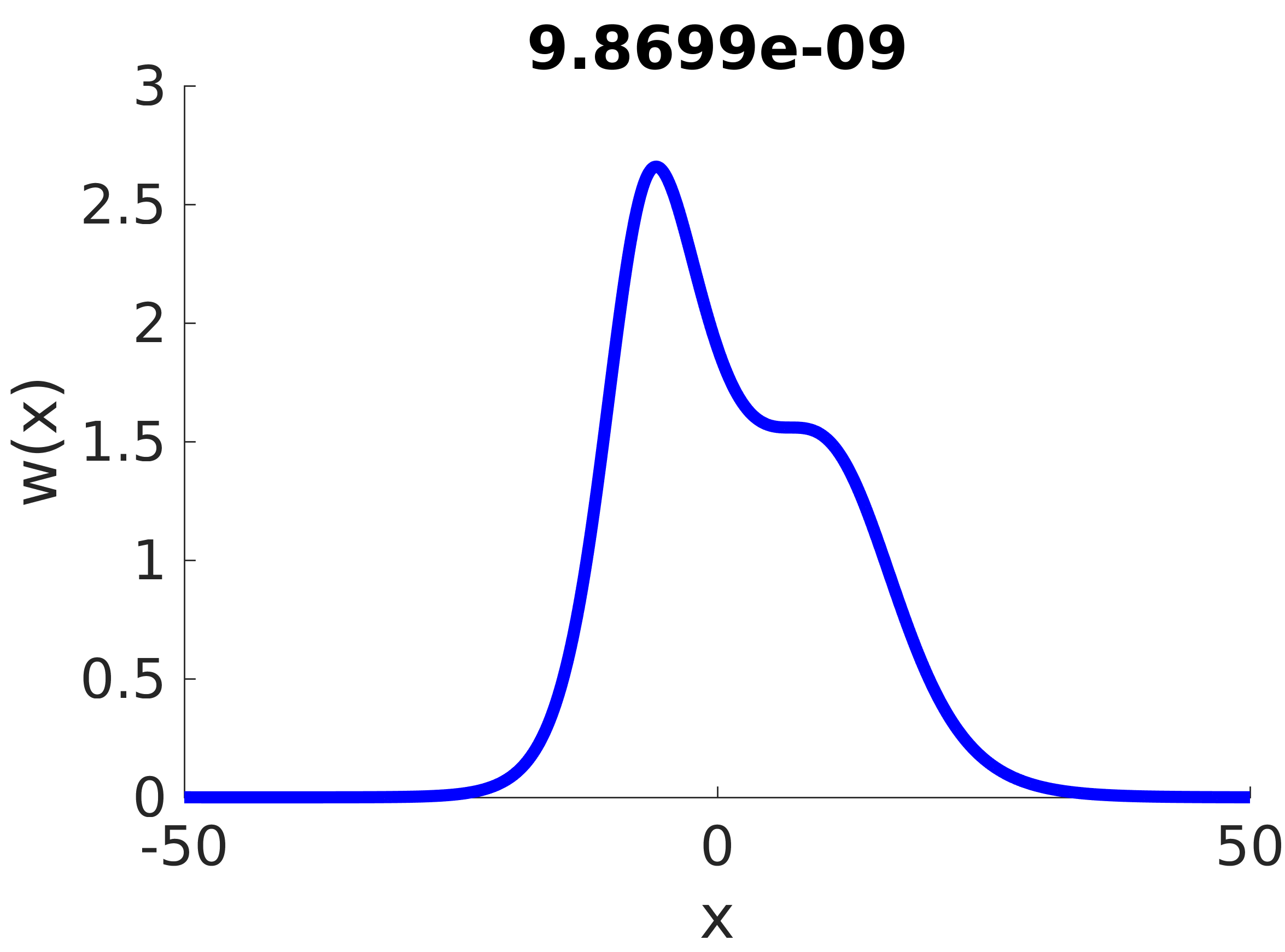
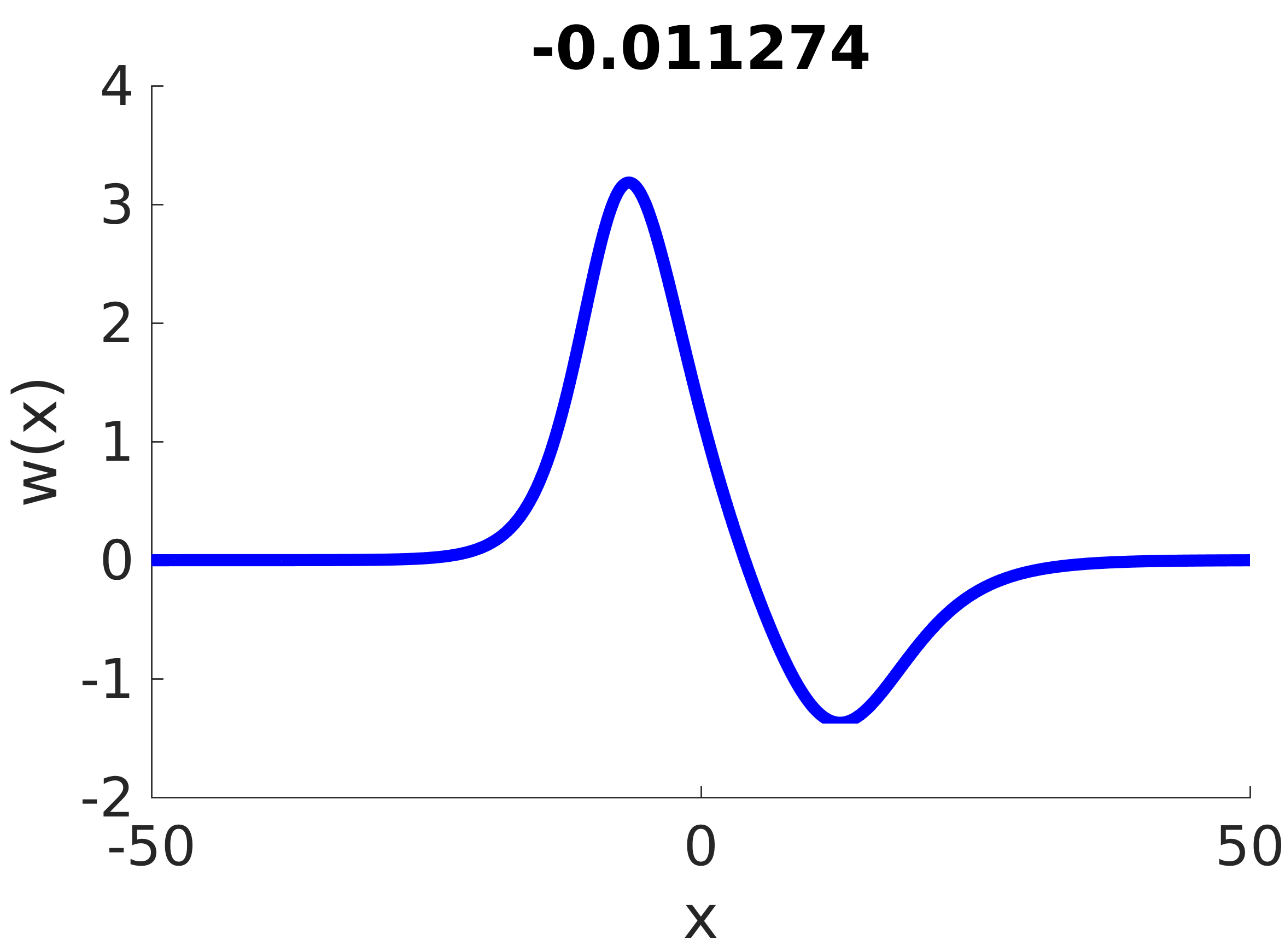
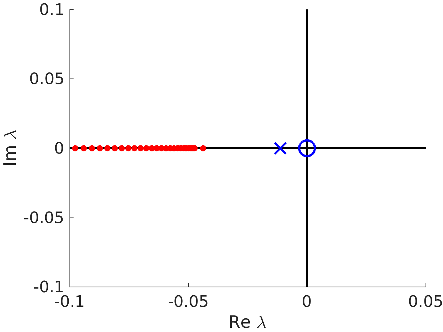
Figure 2.3(a) shows the part of the spectrum of the quintic Nagumo wave which is guaranteed by Proposition 2.2 and 2.3. It is subdivided into the symmetry set $\sigma_{\mathrm{sym}}(\mathcal{P})$ (blue circle), which is determined by Proposition 2.2 and belongs to the point spectrum $\sigma_{\mathrm{pt}}(\mathcal{P})$, and the dispersion set $\sigma_{\mathrm{disp}}(\mathcal{P})$ (red lines), which is determined by Proposition 2.3 and belongs to the essential spectrum $\sigma_{\mathrm{ess}}(\mathcal{P})$. In general, there may be further essential spectrum in $\sigma_{\mathrm{ess}}(\mathcal{P})\setminus\sigma_{\mathrm{disp}}(\mathcal{P})$ and further isolated eigenvalues in $\sigma_{\mathrm{pt}}(\mathcal{P})\setminus\sigma_{\mathrm{sym}}(\mathcal{P})$. In fact, for the quintic Nagumo wave equation we find an extra eigenvalue with negative real part, cf. Figure 2.4(c). The numerical spectrum of the quintic Nagumo wave equation on the spatial domain $[-R,R]$ equipped with periodic boundary conditions is shown in Figure 2.3(b) for $R=50$ and in Figure 2.3(c) for $R=400$. Each of them consists of the approximations of the point spectrum subdivided into the symmetry set (blue circle) and an additional isolated eigenvalue (blue plus sign), and of the essential spectrum (red dots). The missing line inside the ellipse in Figure 2.3(b) gradually appears numerically when enlarging the spatial domain, see Figure 2.3(c). The second ellipse only develops on even larger domains.

3. Rotating waves in several space dimensions

3.1. Freezing rotating waves.

Consider the Cauchy problem associated with (1.5)

(3.1a) $$Mu_{tt}+Bu_{t}=A\triangle u+f(u), \,x\in\mathbb{R}^{d},\,t>0,$$

(3.1b) $$u(\cdot,0)=u_{0},\quad u_{t}(\cdot,0)=v_{0}, \,x\in\mathbb{R}^{d},\,t=0,$$

for some initial data $u_{0},v_{0}:\mathbb{R}^{d}\rightarrow\mathbb{R}^{m}$, where $u_{0}$ denotes the initial displacement and $v_{0}$ the initial velocity. The damped wave equation (3.1) has a more special nonlinearity than in the one-dimensional case, see (1.5). This will simplify some of the computations below.

In the following, let $\mathrm{SE}(d)=\mathrm{SO}(d)\ltimes\mathbb{R}^{d}$ denote the special Euclidean group and $\mathrm{SO}(d)$ the special orthogonal group. Let us introduce new unknowns $(Q(t),\tau(t))\in\mathrm{SE}(d)$ and $v(\xi,t)\in\mathbb{R}^{m}$ via the rotating wave ansatz

(3.2) $$u(x,t) =v(\xi,t),\quad\xi:=Q(t)^{\top}(x-\tau(t)),\,x\in\mathbb{R}^{d},\,t\geqslant 0.$$

Inserting (3.2) into (3.1a) and suppressing arguments of $u$ and $v$ leads to

(3.3) $$\triangle_{x}u= \triangle_{\xi}v,\quad f(u)=f(v),\quad u_{t}=v_{\xi}\left(Q_{t}^{\top}(x-\tau)-Q^{\top}\tau_{t}\right)+v_{t},$$

$$u_{tt}= v_{\xi\xi}\left(Q_{t}^{\top}(x-\tau)-Q^{\top}\tau_{t}\right)^{2}+v_{\xi}\left(Q_{tt}^{\top}(x-\tau)-2Q_{t}^{\top}\tau_{t}-Q^{\top}\tau_{tt}\right)$$

$$+ 2v_{\xi t}\left(Q_{t}^{\top}(x-\tau)-Q^{\top}\tau_{t}\right)+v_{tt}.$$

Hence equation (3.1a) turns into

(3.4) $$\begin{split}&Mv_{tt}+Bv_{t}=A\triangle v-Mv_{\xi\xi}\left(Q_{t}^{\top}Q\xi-Q^{\top}\tau_{t}\right)^{2}-2Mv_{\xi t}\left(Q_{t}^{\top}Q\xi-Q^{\top}\tau_{t}\right)\\ &\quad\quad\quad\quad\quad\quad-Mv_{\xi}\left(Q_{tt}^{\top}Q\xi-2Q_{t}^{\top}\tau_{t}-Q^{\top}\tau_{tt}\right)-Bv_{\xi}\left(Q_{t}^{\top}Q\xi-Q^{\top}\tau_{t}\right)+f(v).\end{split}$$

It is convenient to introduce time-dependent functions $S_{1}(t),S_{2}(t)\in\mathbb{R}^{d,d}$, $\mu_{1}(t),\mu_{2}(t)\in\mathbb{R}^{d}$ via

$$S_{1}:=Q^{\top}Q_{t},\quad S_{2}:=S_{1,t},\quad\mu_{1}:=Q^{\top}\tau_{t},\quad\mu_{2}:=\mu_{1,t}.$$

Obviously, $S_{1}$ and $S_{2}$ satisfy $S_{1}^{\top}=-S_{1}$ and $S_{2}^{\top}=-S_{2}$, which follows from $Q^{\top}Q=I_{d}$ by differentiation. Moreover, we obtain

$$Q_{t}^{\top}Q=-S_{1},\quad Q^{\top}\tau_{t}=\mu_{1},\quad Q_{t}^{\top}\tau_{t}+Q^{\top}\tau_{tt}=\mu_{2},$$

$$Q_{tt}^{\top}Q=-S_{1,t}-S_{1}^{\top}S_{1}=-S_{2}+S_{1}^{2},\quad-Q_{t}^{\top}\tau_{t}=-Q_{t}^{\top}QQ^{\top}\tau_{t}=S_{1}\mu_{1},$$

which transforms (3.4) into the system

(3.5a) $$Mv_{tt}+Bv_{t}=A\triangle v-Mv_{\xi\xi}\left(S_{1}\xi+\mu_{1}\right)^{2}+2Mv_{\xi t}\left(S_{1}\xi+\mu_{1}\right)$$

$$\quad\quad\quad\quad\quad\quad+Mv_{\xi}\left((S_{2}-S_{1}^{2})\xi-S_{1}\mu_{1}+\mu_{2}\right)+Bv_{\xi}\left(S_{1}\xi+\mu_{1}\right)+f(v),$$

(3.5b) $$\begin{pmatrix}S_{1}\\ \mu_{1}\end{pmatrix}_{t}=\begin{pmatrix}S_{2}\\ \mu_{2}\end{pmatrix},$$

(3.5c) $$\begin{pmatrix}Q\\ \tau\end{pmatrix}_{t}=\begin{pmatrix}QS_{1}\\ Q\mu_{1}\end{pmatrix}.$$

The quantity $(Q(t),\tau(t))$ describes the position by its spatial shift $\tau(t)$ and the rotation $Q(t)$. Moreover, $S_{1}(t)$ denotes the rotational velocities, $\mu_{1}(t)$ the translational velocities, $S_{2}(t)$ the angular acceleration and $\mu_{2}(t)$ the translational acceleration of the rotating wave $v$ at time $t$. Note that in contrast to the traveling waves the leading part $A\triangle-M\partial_{\xi}^{2}(\cdot)(S_{1}\xi+\mu_{1})^{2}$ not only depends on the velocities $S_{1}$ and $\mu_{1}$, but also on the spatial variable $\xi$, which means that the leading part has unbounded (linearly growing) coefficients. We next specify initial data for the system (3.5) as follows,

(3.6) $$\begin{split}&\quad v(\cdot,0)=u_{0},\quad v_{t}(\cdot,0)=v_{0}+u_{0,\xi}(S_{1}^{0}\xi+\mu_{1}^{0}),\\ &S_{1}(0)=S_{1}^{0},\quad\mu_{1}(0)=\mu_{1}^{0},\quad Q(0)=I_{d},\quad\tau(0)=0.\end{split}$$

Note that, requiring $Q(0)=I_{d}$, $\tau(0)=0$, $S_{1}(0)=S_{1}^{0}$ and $\mu_{1}(0)=\mu_{1}^{0}$ for some $S_{1}^{0}\in\mathbb{R}^{d,d}$ with $(S_{1}^{0})^{\top}=-S_{1}^{0}$ and $\mu_{1}^{0}\in\mathbb{R}^{d}$, the first equation in (3.6) follows from (3.2) and (3.1b), while the second condition in (3.6) can be deduced from (3.3), (3.1b), (3.5c) and the first condition in (3.6).

The system (3.5) comprises evolution equations for the unknowns $v$, $S$ and $\mu_{1}$. In order to specify the remaining variables $S_{2}$ and $\mu_{2}$ we impose $\mathrm{dim}\,\mathrm{SE}(d)=\frac{d(d+1)}{2}$ additional scalar algebraic constraints, also known as phase conditions

(3.7) $$\psi(v,v_{t},(S_{1},\mu_{1}),(S_{2},\mu_{2}))=0\in\mathbb{R}^{\frac{d(d+1)}{2}},\quad t\geqslant 0.$$

Two possible choices of such a phase condition are

(3.8) $$\psi_{\mathrm{fix}}(v):=\begin{pmatrix}\langle v-\hat{v},D_{l}\hat{v}\rangle_{L^{2}}\\ \langle v-\hat{v},D^{(i,j)}\hat{v}\rangle_{L^{2}}\end{pmatrix}=0,\;t\geqslant 0,$$

(3.9) $$\psi_{\mathrm{orth}}(v,v_{t}):=\begin{pmatrix}\langle v_{t},D_{l}v\rangle_{L^{2}}\\ \langle v_{t},D^{(i,j)}v\rangle_{L^{2}}\end{pmatrix}=0,\;t\geqslant 0,$$

for $l=1,\ldots,d$, $i=1,\ldots,d-1$ and $j=i+1,\ldots,d$ with $D_{l}:=\partial_{\xi_{l}}$ and $D^{(i,j)}:=\xi_{j}\partial_{\xi_{i}}-\xi_{i}\partial_{\xi_{j}}$. Condition (3.8) is obtained from the requirement that the distance

$$\rho(Q,\tau):=\left\|v(\cdot,t)-\hat{v}(Q^{\top}(\cdot-\tau))\right\|^{2}_{L^{2}}$$

attains a local minimum at $(Q,\tau)=(I_{d},0)$. Since $D_{l},D^{(i,j)}$ are the generators of the Euclidean group action, condition (3.9) requires the time derivative of $v$ to be orthogonal to the group orbit of $v$ at any time instance.

Combining the differential equations (3.5), the initial data (3.6) and the phase condition (3.7), we obtain the following partial differential algebraic evolution equation (PDAE)

(3.10a) $$Mv_{tt}+Bv_{t}=A\triangle v-Mv_{\xi\xi}\left(S_{1}\xi+\mu_{1}\right)^{2}+2Mv_{\xi t}\left(S_{1}\xi+\mu_{1}\right)$$

$$\quad\quad\quad\quad\quad\quad+Mv_{\xi}\left((S_{2}-S_{1}^{2})\xi-S_{1}\mu_{1}+\mu_{2}\right)+Bv_{\xi}\left(S_{1}\xi+\mu_{1}\right)+f(v), \,\xi\in\mathbb{R}^{d},\,t>0,$$

(3.10b) $$v(\cdot,0)=u_{0},\quad v_{t}(\cdot,0)=v_{0}+u_{0,\xi}(S_{1}^{0}\xi+\mu_{1}^{0}), \,\xi\in\mathbb{R}^{d},\,t=0,$$

(3.10c) $$0=\psi(v,v_{t},(S_{1},\mu_{1}),(S_{2},\mu_{2})), \,t\geqslant 0,$$

(3.10d) $$\begin{pmatrix}S_{1}\\ \mu_{1}\end{pmatrix}_{t}=\begin{pmatrix}S_{2}\\ \mu_{2}\end{pmatrix},\quad\begin{pmatrix}S_{1}(0)\\ \mu_{1}(0)\end{pmatrix}=\begin{pmatrix}S_{1}^{0}\\ \mu_{1}^{0}\end{pmatrix}, \,t\geqslant 0,$$

(3.10e) $$\begin{pmatrix}Q\\ \tau\end{pmatrix}_{t}=\begin{pmatrix}QS_{1}\\ Q\mu_{1}\end{pmatrix},\quad\begin{pmatrix}Q(0)\\ \tau(0)\end{pmatrix}=\begin{pmatrix}I_{d}\\ 0\end{pmatrix}, \,t\geqslant 0.$$

The system (3.10) depends on the choice of phase condition and must be solved for $(v,S_{1},\mu_{1},S_{2},\mu_{2},Q,\tau)$ for given $(u_{0},v_{0},S_{1}^{0},\mu_{1}^{0})$. It consists of a PDE for $v$ in (3.10a)–(3.10b), two systems of ODEs for $(S_{1},\mu_{1})$ in (3.10d) and for $(Q,\tau)$ in (3.10e) and $\frac{d(d+1)}{2}$ algebraic constraints for $(S_{2},\mu_{2})$ in (3.10c). The ODE (3.10e) for $(Q,\tau)$ is the reconstruction equation (see [24]), it decouples from the other equations in (3.10) and can be solved in a postprocessing step. Note that in the frozen equation for first order evolution equations, the ODE for $(S_{1},\mu_{1})$ does not appear, see [17, (10.26)]. The additional ODE is a new component of the PDAE and is caused by the second order time derivative.

Finally, note that $(v,S_{1},\mu_{1},S_{2},\mu_{2})=(v_{\star},S_{\star},\mu_{\star},0,0)$ satisfies

$$0=A\triangle v-Mv_{\star,\xi\xi}\left(S_{\star}\xi+\mu_{\star}\right)^{2}-Mv_{\star,\xi}S_{\star}\left(S_{\star}\xi+\mu_{\star}\right)+Bv_{\star,\xi}\left(S_{\star}\xi+\mu_{\star}\right)+f(v_{\star}),\,\xi\in\mathbb{R}^{d},$$

$$0=\begin{pmatrix}S_{2}\\ \mu_{2}\end{pmatrix}.$$

If, in addition, it has been arranged that $v_{\star},S_{\star},\mu_{\star}$ satisfy the phase condition $\psi(v_{\star},0,S_{\star},\mu_{\star},0,0)=0$ then $(v_{\star},S_{\star},\mu_{\star},0,0)$ is a stationary solution of the system (3.10a),(3.10c),(3.10d). For a stable rotating wave we expect that solutions $(v,S_{1},\mu_{1},S_{2},\mu_{2})$ of (3.10a)–(3.10d) satisfy

$$v(t)\rightarrow v_{\star},\quad(S_{1}(t),\mu_{1}(t))\rightarrow(S_{\star},\mu_{\star}),\quad(S_{2}(t),\mu_{2}(t))\rightarrow(0,0),\quad\text{as}\quad t\to\infty,$$

provided the initial data are close to their limiting values.

Example 3.1 (Cubic-quintic complex Ginzburg-Landau wave equation).

Consider the cubic-quintic complex Ginzburg-Landau wave equation

(3.11) $$\varepsilon u_{tt}+\rho u_{t}=\alpha\triangle u+u(\delta+\beta|u|^{2}+\gamma|u|^{4}),\;x\in\mathbb{R}^{d},\,t\geqslant 0$$

with $u=u(x,t)\in\mathbb{C}$, $d\in\{2,3\}$, $\varepsilon,\rho,\alpha,\beta,\gamma,\delta\in\mathbb{C}$ and $\mathrm{Re}\,\alpha>0$. For the parameter values

(3.12) $$\varepsilon=10^{-4},\quad\rho=1,\quad\alpha=\frac{3}{5},\quad\gamma=-1-\frac{1}{10}i,\quad\beta=\frac{5}{2}+i,\quad\delta=-0.73.$$

equation (3.11) admits a spinning soliton solution.

Figure 3.1. Solution of cubic-quintic complex Ginzburg-Landau wave equation (3.11): Spinning soliton $u(x,t)$ at time $t=50$ (a) and its time evolution along $x_{2}=0$ (b) for parameters from (3.12).

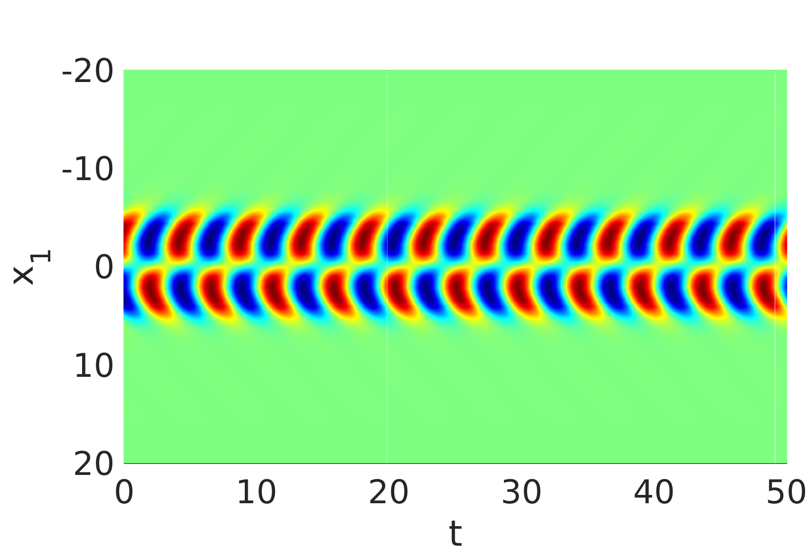
Figure 3.1 shows a numerical simulation of the solution $u$ of (3.11) on the ball $B_{R}(0)$ of radius $R=20$, with homogeneous Neumann boundary conditions and with parameter values from (3.12). The initial data $u_{0}$ and $v_{0}$ are generated in the following way. First we use the freezing method to compute a rotating wave in the parabolic case (as in [17]) for parameter values $\varepsilon=0$, $\rho=1$ and

$$\alpha=\frac{1}{2}+\frac{1}{2}i,\quad\gamma=-1-\frac{1}{10}i,\quad\beta=\frac{5}{2}+i,\quad\delta=-\frac{1}{2}.$$

Then the parameter set $(\varepsilon,\alpha,\delta)$ is gradually changed until the values (3.12) are attained. For the space discretization we use continuous piecewise linear finite elements with spatial stepsize $\triangle x=0.8$. For the time discretization we use the BDF method of order $2$ with absolute tolerance $\mathrm{atol}=10^{-4}$, relative tolerance $\mathrm{rtol}=10^{-3}$, temporal stepsize $\triangle t=0.1$ and final time $T=50$. Computations are performed with the help of the software COMSOL 5.2.

Let us now consider the frozen cubic-quintic complex Ginzburg-Landau wave equation resulting from (3.10)

(3.13a) $$\varepsilon v_{tt}+\rho v_{t}=\alpha\triangle v-\varepsilon v_{\xi\xi}\left(S_{1}\xi+\mu_{1}\right)^{2}+2\varepsilon v_{\xi t}\left(S_{1}\xi+\mu_{1}\right)$$

$$\quad\quad\quad\quad\quad\quad+\varepsilon v_{\xi}\left((S_{2}-S_{1}^{2})\xi-S_{1}\mu_{1}+\mu_{2}\right)+\rho v_{\xi}\left(S_{1}\xi+\mu_{1}\right)+f(v), \,\xi\in\mathbb{R}^{d},\,t>0,$$

(3.13b) $$v(\cdot,0)=u_{0},\quad v_{t}(\cdot,0)=v_{0}+u_{0,\xi}(S_{1}^{0}\xi+\mu_{1}^{0}), \,\xi\in\mathbb{R}^{d},\,t=0,$$

(3.13c) $$0=\psi_{\mathrm{fix}}(v):=\begin{pmatrix}\langle v-\hat{v},D_{l}\hat{v}\rangle_{L^{2}}\\ \langle v-\hat{v},D^{(i,j)}\hat{v}\rangle_{L^{2}}\end{pmatrix}, \,t\geqslant 0,$$

(3.13d) $$\begin{pmatrix}S_{1}\\ \mu_{1}\end{pmatrix}_{t}=\begin{pmatrix}S_{2}\\ \mu_{2}\end{pmatrix},\quad\begin{pmatrix}S_{1}(0)\\ \mu_{1}(0)\end{pmatrix}=\begin{pmatrix}S_{1}^{0}\\ \mu_{1}^{0}\end{pmatrix}, \,t\geqslant 0,$$

(3.13e) $$\begin{pmatrix}Q\\ \tau\end{pmatrix}_{t}=\begin{pmatrix}QS_{1}\\ Q\mu_{1}\end{pmatrix},\quad\begin{pmatrix}Q(0)\\ \tau(0)\end{pmatrix}=\begin{pmatrix}I_{d}\\ 0\end{pmatrix}, \,t\geqslant 0.$$

Figure 3.2. Solution of the frozen cubic-quintic complex Ginzburg-Landau wave equation (3.13): profile $v(x,t)$ at time $t=2000$ (a), its time evolution along $x_{2}=0$ (b), velocities $\mu_{1}(t)$ (c), and accelerations $\mu_{2}(t)$ (d) for parameters from (3.12).

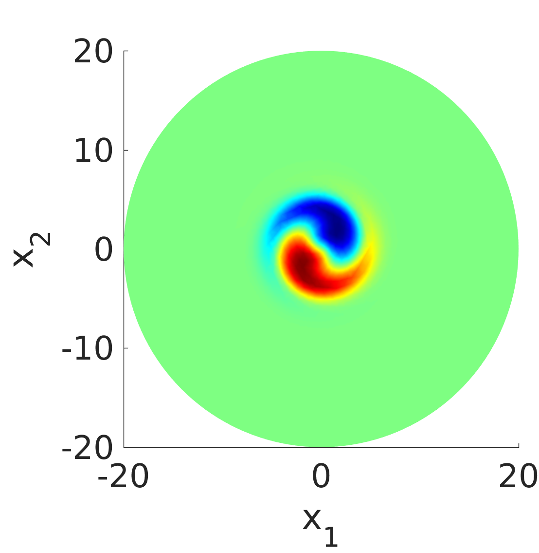
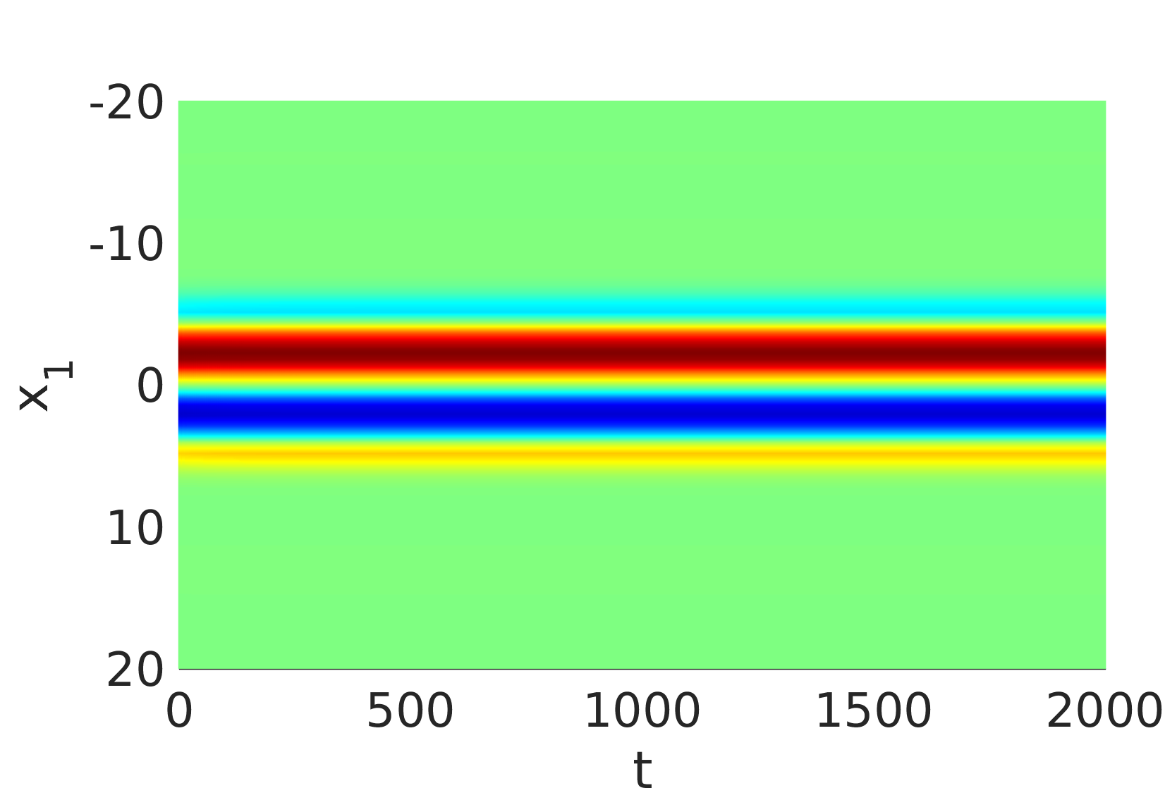
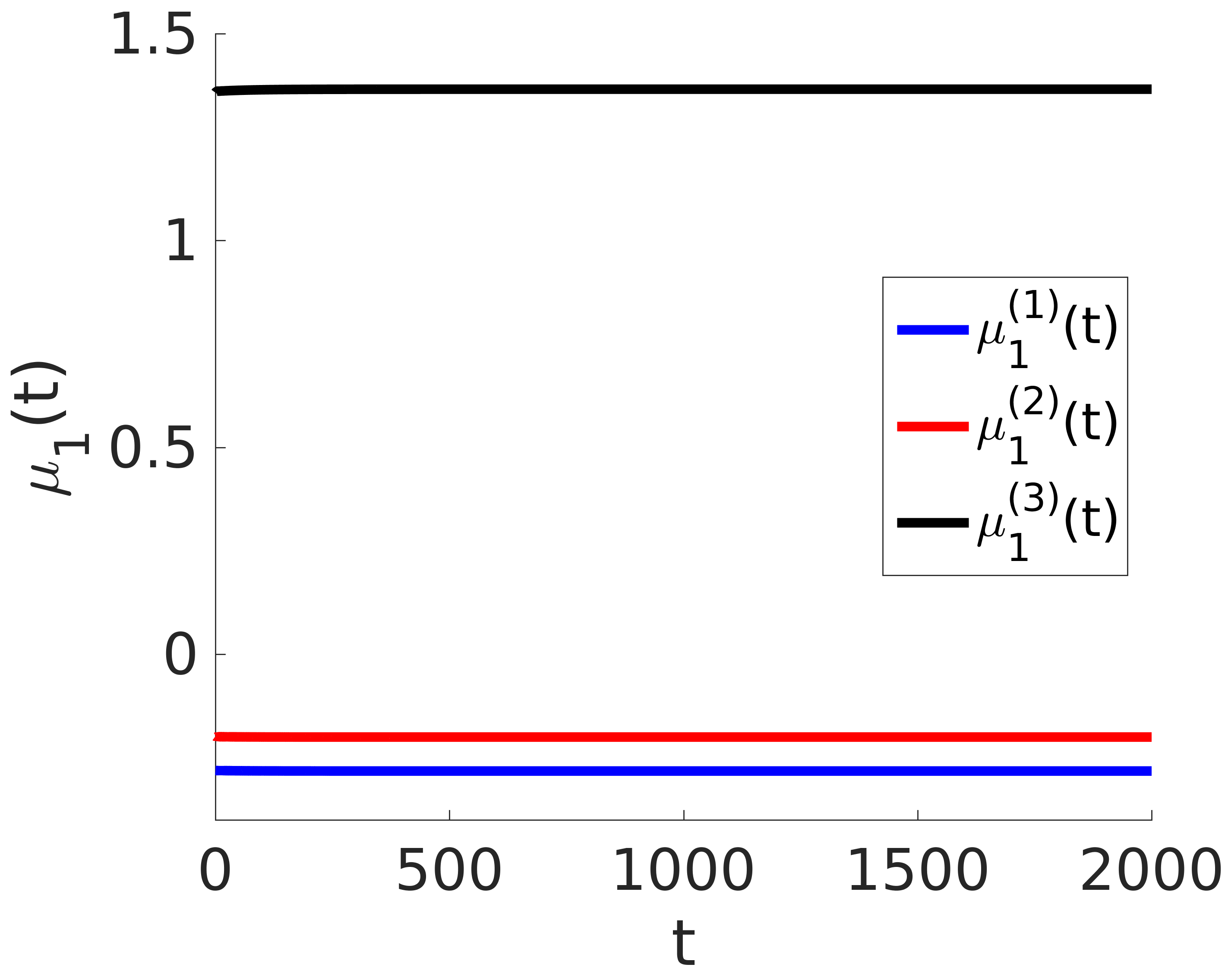
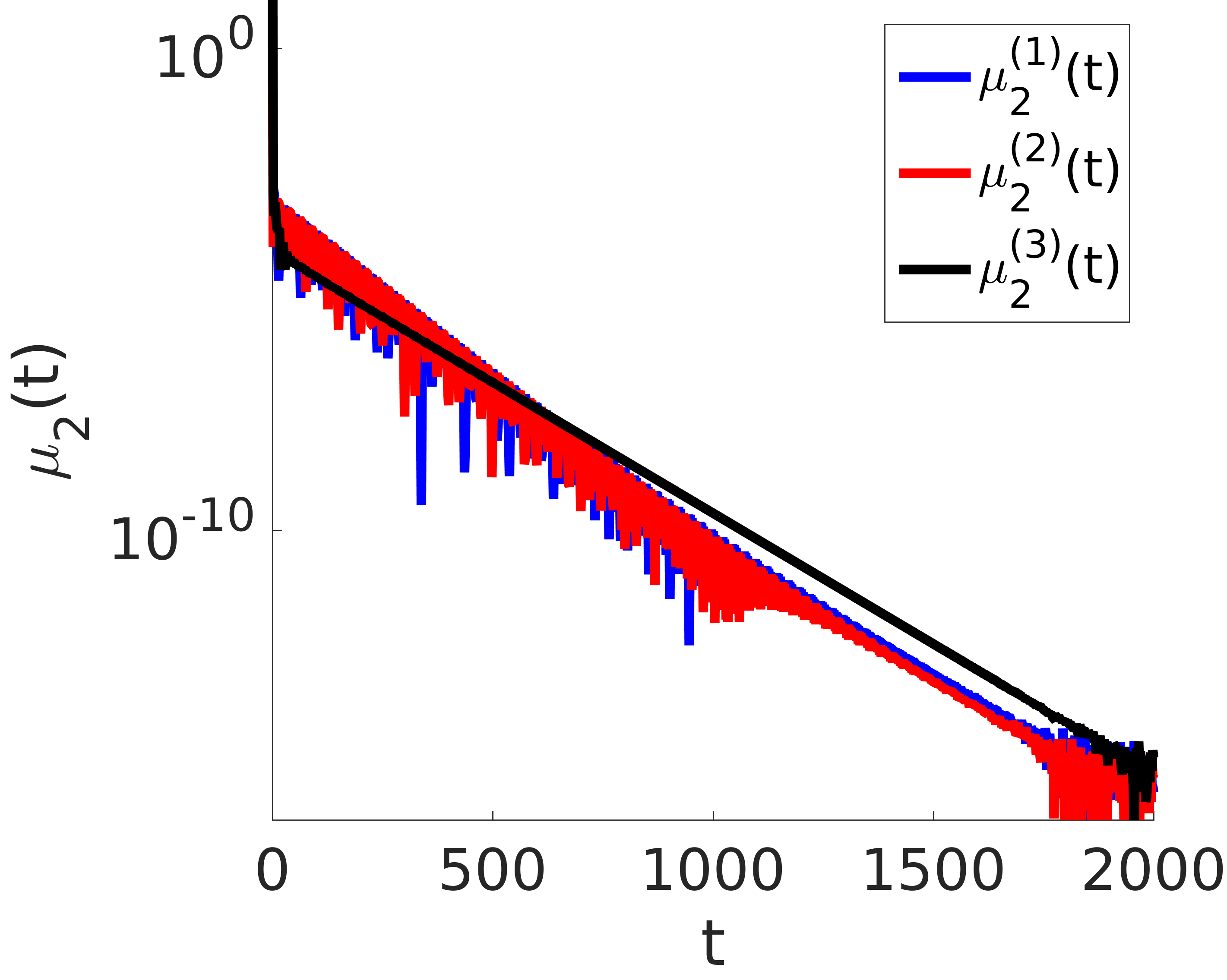
Figure 3.2 shows the solution $(v,S_{1},\mu_{1},S_{2},\mu_{2},Q,\tau)$ of (3.13) on the ball $B_{R}(0)$ with radius $R=20$, homogeneous Neumann boundary conditions, initial data $u_{0}$, $v_{0}$ as in the nonfrozen case, and reference function $\hat{v}=u_{0}$. For the computation we used the fixed phase condition $\psi_{\mathrm{fix}}(v)$ from (3.8). The spatial discretization data are taken as in the nonfrozen case. For the time discretization we used the BDF method of order $2$ with absolute tolerance $\mathrm{atol}=10^{-3}$, relative tolerance $\mathrm{rtol}=10^{-2}$, maximal temporal stepsize $\triangle t=0.5$, initial step $10^{-4}$, and final time $T=2000$. Due to the choice of initial data, the profile becomes immediately stationary, the acceleration $\mu_{2}$ converges to zero, while the speed $\mu_{1}$ and the nontrivial entry $S_{12}$ of $S$ approach asymptotic values

$$\mu_{1}^{(1)}=-0.2819,\quad\mu_{1}^{(2)}=-0.1999,\quad S_{12}=1.3658.$$

Note that we have a clockwise rotation if $S_{12}>0$, and a counter clockwise rotation if $S_{12}<0$. Thus, the spinning soliton rotates clockwise. The center of rotation $x_{\star}$ and the temporal period $T^{\mathrm{2D}}$ for one rotation are given by, see [17, Exa.10.8],

$$x_{\star}=\frac{1}{S_{12}}\begin{pmatrix}\mu_{1}^{(2)}\\ -\mu_{1}^{(1)}\end{pmatrix}=\begin{pmatrix}-0.1464\\ 0.2064\end{pmatrix},\quad\quad T^{\mathrm{2D}}=\frac{2\pi}{|S_{12}|}=4.6004.$$

3.2. Spectra of rotating waves.

Consider the linearized equation

(3.14) $$Mv_{tt}+Bv_{t}-A\triangle v+Mv_{\xi\xi}(S_{\star}\xi)^{2}-2Mv_{\xi t}S_{\star}\xi+Mv_{\xi}S_{\star}^{2}\xi-Bv_{\xi}S_{\star}\xi-Df(v_{\star})v=0.$$

Equation (3.14) is obtained from the co-rotating frame equation (1.6) when linearizing at the profile $v_{\star}$. Moreover, we assume $\mu_{\star}=0$, that is the wave rotates about the origin. Shifting the center of rotation does not influence the stability properties, see the discussion in [4]. Looking for solutions of the form $v(\xi,t)=e^{\lambda t}w(\xi)$ to (3.14) yields the quadratic eigenvalue problem

(3.15) $$\mathcal{P}(\lambda)w:=\left(\lambda^{2}P_{2}+\lambda P_{1}+P_{0}\right)w=0,\,\xi\in\mathbb{R}^{d}$$

with differential operators $P_{j}$ defined by

(3.16) $$\begin{split}P_{2}=&M,\quad P_{1}=B-2M\left(\partial_{\xi}\,\cdot\right)S_{\star}\xi=B-2M\sum_{j=1}^{d}(S_{\star}\xi)_{j}\partial_{\xi_{j}},\\ P_{0}=&-A\triangle\,\cdot+M\left(\partial_{\xi}^{2}\,\cdot\right)(S_{\star}\xi)^{2}+M\left(\partial_{\xi}\,\cdot\right)S_{\star}^{2}\xi-B\left(\partial_{\xi}\,\cdot\right)S_{\star}\xi-Df(v_{\star})\,\cdot\\ =&-A\sum_{j=1}^{d}\partial_{\xi_{j}}^{2}+M\sum_{j=1}^{d}\sum_{\nu=1}^{d}(S_{\star}\xi)_{j}(S_{\star}\xi)_{\nu}\partial_{\xi_{j}}\partial_{\xi_{\nu}}+M\sum_{j=1}^{d}(S_{\star}^{2}\xi)_{j}\partial_{\xi_{j}}-B\sum_{j=1}^{d}(S_{\star}\xi)_{j}\partial_{\xi_{j}}-Df(v_{\star}).\end{split}$$

As in the one-dimensional case we cannot solve equation (3.15) in general. Rather, our aim is to determine the symmetry set $\sigma_{\mathrm{sym}}(\mathcal{P})$ as a subset of the point spectrum $\sigma_{\mathrm{pt}}(\mathcal{P})$, and the dispersion set $\sigma_{\mathrm{disp}}(\mathcal{P})$ as a subset of the essential spectrum $\sigma_{\mathrm{ess}}(\mathcal{P})$. The point spectrum is affected by the underlying group symmetries while the essential spectrum depends on the far-field behavior of the wave.

In the following we present the recipe for computing the subsets $\sigma_{\mathrm{sym}}(\mathcal{P})\subseteq\sigma_{\mathrm{pt}}(\mathcal{P})$ and $\sigma_{\mathrm{disp}}(\mathcal{P})\subseteq\sigma_{\mathrm{ess}}(\mathcal{P})$.

Point Spectrum and symmetry set.

Let us look for eigenfunctions $w$ of (3.15) of the form

(3.17) $$w(\xi)=v_{\star,\xi}(\xi)(E\xi+b)\quad\quad\text{for some $E\in\mathbb{C}^{d,d}$, $b\in\mathbb{C}^{d}$, $E^{\top}=-E$, $v_{\star}\in C^{3}(\mathbb{R}^{d},\mathbb{R}^{m})$.}$$

This ansatz is motivated by the fact that functions of this type span the image of the derivative of the group action $(Q,\tau)\rightarrow v_{\star}(Q^{\top}(\cdot-\tau))$ at the unit element $(Q,\tau)=(I_{d},0)\in\mathrm{SE}(d)$ (compare (3.2)). We plug (3.17) into (3.15) and use the equalities

$$Mw=Mv_{\star,\xi}(E\xi+b),\quad\quad Bw=Bv_{\star,\xi}(E\xi+b),$$

(3.18) $$2M(\partial_{\xi}w)S_{\star}\xi=2Mv_{\star,\xi\xi}(E\xi+b)S_{\star}\xi+2Mv_{\star,\xi}ES_{\star}\xi$$

(3.19) $$A\triangle w=(\partial_{\xi}(A\triangle v_{\star}))(E\xi+b)$$

(3.20) $$M(\partial_{\xi}^{2}w)(S_{\star}\xi)^{2}=(\partial_{\xi}(Mv_{\star,\xi\xi}(S_{\star}\xi)^{2}))(E\xi+b)+2Mv_{\star,\xi\xi}([E,S_{\star}]\xi-S_{\star}b)S_{\star}\xi,$$

(3.21) $$M(\partial_{\xi}w)S_{\star}^{2}\xi=(\partial_{\xi}(Mv_{\star,\xi}S_{\star}^{2}\xi))(E\xi+b)+Mv_{\star,\xi}([E,S_{\star}^{2}]\xi-S_{\star}^{2}b),$$

(3.22) $$B(\partial_{\xi}w)S_{\star}\xi=(\partial_{\xi}(Bv_{\star,\xi}S_{\star}\xi))(E\xi+b)+Bv_{\star,\xi}([E,S_{\star}]\xi-S_{\star}b),$$

(3.23) $$Df(v_{\star})w=(\partial_{\xi}(f(v_{\star})))(E\xi+b)$$

where $[E,S_{\star}]:=ES_{\star}-S_{\star}E$ is the Lie bracket. This leads to the following equation:

$$0= \lambda^{2}Mv_{\star,\xi}(E\xi+b)+\lambda\Big{(}Bv_{\star,\xi}(E\xi+b)-2Mv_{\star,\xi\xi}(E\xi+b)S_{\star}\xi-2Mv_{\star,\xi}ES_{\star}\xi\Big{)}$$

(3.24) $$+\Big{(}2Mv_{\star,\xi\xi}([E,S_{\star}]\xi-S_{\star}b)S_{\star}\xi+Mv_{\star,\xi}([E,S_{\star}^{2}]\xi-S_{\star}^{2}b)-Bv_{\star,\xi}([E,S_{\star}]\xi-S_{\star}b)$$

$$\;\;\quad\;-\partial_{\xi}\big{(}A\triangle v_{\star}-Mv_{\star,\xi\xi}(S_{\star}\xi)^{2}-Mv_{\star,\xi}S_{\star}^{2}\xi+Bv_{\star,\xi}S_{\star}\xi+f(v_{\star})\big{)}(E\xi+b)\Big{)}.$$

Now we use the rotating wave equation (1.8) in (3.2.1) and obtain by rearranging the remaining terms

$$0= Mv_{\star,\xi}\Big{(}\lambda^{2}(E\xi+b)-2\lambda ES_{\star}\xi+[E,S_{\star}^{2}]\xi-S_{\star}^{2}b\Big{)}+Bv_{\star,\xi}\Big{(}\lambda(E\xi+b)-[E,S_{\star}]\xi+S_{\star}b\Big{)}$$

(3.25) $$-2Mv_{\star,\xi\xi}\Big{(}\lambda(E\xi+b)-[E,S_{\star}]\xi+S_{\star}b\Big{)}S_{\star}\xi$$

$$= Mv_{\star,\xi}\Big{(}(\lambda^{2}E-2\lambda ES_{\star}+[E,S_{\star}^{2}])\xi+\lambda^{2}b-S_{\star}^{2}b\Big{)}+Bv_{\star,\xi}\Big{(}(\lambda E-[E,S_{\star}])\xi+\lambda b+S_{\star}b\Big{)}$$

$$-2Mv_{\star,\xi\xi}\Big{(}(\lambda E-[E,S_{\star}])\xi+\lambda b+S_{\star}b\Big{)}S_{\star}\xi.$$

Comparing coefficients in (3.2.1) yields the finite-dimensional eigenvalue problem (see [9],[17], [3])

(3.26a) $$\lambda E =[E,S_{\star}],$$

(3.26b) $$\lambda b =-S_{\star}b,$$

which must be solved for $(\lambda,E,b)$ and admits $\frac{d(d+1)}{2}$ solutions. In fact, having a solution $(\lambda,E,b)$ of (3.26), then the last two terms in (3.2.1) obviously vanish. The first term vanishes if we write both summands as

$$\lambda^{2}b-S_{\star}^{2}b=\lambda(\lambda b+S_{\star}b)-S_{\star}(\lambda b+S_{\star}b)$$

and

$$\lambda^{2}E-2\lambda ES_{\star}+[E,S_{\star}^{2}]=\lambda(\lambda E-[E,S_{\star}])-(2\lambda ES_{\star}-\lambda[E,S_{\star}]-[E,S_{\star}^{2}])$$

$$= \lambda(\lambda E-[E,S_{\star}])-\left((\lambda E-[E,S_{\star}])S_{\star}+S_{\star}(\lambda E-[E,S_{\star}])+[E,S_{\star}]S_{\star}+S_{\star}[E,S_{\star}]-[E,S_{\star}^{2}]\right),$$

and use the identity $[E,S_{\star}]S_{\star}+S_{\star}[E,S_{\star}]-[E,S_{\star}^{2}]=[E,[S_{\star},S_{\star}]]=0$ which holds by skew-symmetry of $S_{\star}$. Therefore, it is sufficient to solve (3.26). Furthermore, if $(\lambda,E)$ is a solution of (3.26a), then $(\lambda,E,0)$ solves (3.26), and, similarly, if $(\lambda,b)$ is a solution of (3.26b), then $(\lambda,0,b)$ solves (3.26). Therefore, it is sufficient to solve (3.26a) and (3.26b) separately. For the skew-symmetric matrix $S_{\star}$ we have $S_{\star}=U\Lambda U^{{\mathsf{H}}}$ for some unitary $U\in C^{d,d}$ and some diagonal matrix $\Lambda=\mathrm{diag}(\lambda_{1},\ldots,\lambda_{d})$ where $\lambda_{1},\ldots,\lambda_{d}\in i\mathbb{R}$ are the eigenvalues of $S_{\star}$. In particular, this implies $S_{\star}^{\top}=\overline{U}\Lambda U^{\top}$.

• Multiply (3.26b) from the left by $U^{{\mathsf{H}}}$ and define $\tilde{b}=U^{{\mathsf{H}}}b$ to obtain

  (3.27) $$\lambda\tilde{b}=\lambda U^{{\mathsf{H}}}b=-U^{{\mathsf{H}}}S_{\star}b=-U^{{\mathsf{H}}}U\Lambda U^{{\mathsf{H}}}b=-\Lambda\tilde{b}.$$

  Equation (3.27) has solutions $(\lambda,\tilde{b})=(-\lambda_{l},e_{l})$, hence (3.26b) has solutions $(\lambda,b)=(-\lambda_{l},Ue_{l})$, and (3.26) has solutions $(\lambda,E,b)=(-\lambda_{l},0,Ue_{l})$ for $l=1,\ldots,d$.

• Multiply (3.26a) from the left by $U^{{\mathsf{H}}}$, from the right by $\bar{U}$, define $\tilde{E}=U^{{\mathsf{H}}}E\overline{U}$, and use the skew-symmetry of $S_{\star}$ and $\tilde{E}$, to obtain

  (3.28) $$\lambda\tilde{E}=\lambda U^{{\mathsf{H}}}E\overline{U}=U^{{\mathsf{H}}}[E,S_{\star}]\overline{U}=-U^{{\mathsf{H}}}E\overline{U}\Lambda U^{\top}\overline{U}-U^{{\mathsf{H}}}U\Lambda U^{{\mathsf{H}}}E\overline{U}=-\tilde{E}\Lambda-\Lambda\tilde{E}=\tilde{E}^{\top}\Lambda-\Lambda\tilde{E}.$$

  Equation (3.28) has solutions $(\lambda,\tilde{E})=(-(\lambda_{i}+\lambda_{j}),I_{ij}-I_{ji})$, hence (3.26a) has solutions $(\lambda,E)=(-(\lambda_{i}+\lambda_{j}),U(I_{ij}-I_{ji})U^{\top})$, and (3.26) has solutions $(\lambda,E,b)=(-(\lambda_{i}+\lambda_{j}),U(I_{ij}-I_{ji})U^{\top},0)$ for $i=1,\ldots,d-1$, $j=i+1,\ldots,d$, where $I_{ij}$ has entry $1$ in the $i$th row and $j$th column and $0$ otherwise.

Let us summarize the result in a proposition.

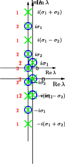
Proposition 3.2 (Point spectrum of rotating waves).

Let $f\in C^{2}(\mathbb{R}^{m},\mathbb{R}^{m})$ and let $v_{\star}\in C^{3}(\mathbb{R}^{d},\mathbb{R}^{m})$ be a classical solution of (1.8) for some skew-symmetric matrix $S_{\star}\in\mathbb{R}^{m,m}$ with eigenvalues denoted by $\lambda_{1},\ldots,\lambda_{d}$ and unitary matrix $U\in\mathbb{C}^{d,d}$ diagonalizing $S_{\star}$. Then

$$w=v_{\star,\xi}(E\xi+b)$$

is a classical solution of the eigenvalue problem (3.15) provided that

$$(\lambda,E,b)=(-\lambda_{l},0,Ue_{l})\quad\quad\text{or}\quad\quad(\lambda,E,b)=(-(\lambda_{i}+\lambda_{j}),U(I_{ij}-I_{ji})U^{\top},0)$$

for some $l=1,\dots,d$, $i=1,\ldots,d-1$, $j=i+1,\ldots,d$. In particular, the symmetry set

$$\sigma_{\mathrm{sym}}(\mathcal{P})=\sigma(S_{\star})\cup\{\lambda_{i}+\lambda_{j}:1\leqslant i<j\leqslant d\}.$$

belongs to the point spectrum $\sigma_{\mathrm{pt}}(\mathcal{P})$ of $\mathcal{P}$.

Altogether, Proposition 3.2 yields $\frac{d(d+1)}{2}$ solutions of the quadratic eigenvalue problem (3.15). It is a remarkable feature that the eigenvalues and the eigenfunctions coincide with those for first order evolution equations, see [3], [17]. Moreover, we suggest that Proposition 3.2 also applies to rotating waves that are not localized, e.g. spiral waves and scroll waves. This has been confirmed in numerical experiments.

Figure 3.3 shows the eigenvalues $\lambda\in\sigma_{\mathrm{sym}}(\mathcal{P})$ from Proposition 3.2 and their corresponding multiplicities for different space dimensions $d=2,3,4,5$. The eigenvalues $\lambda\in\sigma(S_{\star})$ are indicated by blue circles, the eigenvalues $\lambda\in\left\{\lambda_{i}+\lambda_{j}\mid\lambda_{i},\lambda_{j}\in\sigma(S_{\star}),\,1\leqslant i<j\leqslant d\right\}$ by green crosses. The imaginary values to the right of the symbols denote eigenvalues and the numbers to the left their corresponding multiplicities. As expected, there are $\frac{d(d+1)}{2}$ eigenvalues on the imaginary axis in case of space dimension $d$.

(a) $d=2$
$\mathrm{dim}\,\mathrm{SE}(2)=3$

(b) $d=3$
$\mathrm{dim}\,\mathrm{SE}(3)=6$

(c) $d=4$
$\mathrm{dim}\,\mathrm{SE}(4)=10$

(d) $d=5$
$\mathrm{dim}\,\mathrm{SE}(5)=15$

Figure 3.3. Point spectrum of the linearization $\mathcal{P}$ on the imaginary axis $i\mathbb{R}$ for space dimension $d=2,3,4,5$ given by Proposition 3.2.

Essential spectrum and dispersion set.

1. Quasi-diagonal real form. Let us transform the skew-symmetric matrix $S_{\star}$ into quasi-diagonal real form. For this purpose, let $\pm i\sigma_{1},\ldots,\pm i\sigma_{k}$ be the nonzero eigenvalues of $S_{\star}$ so that $0$ is a semisimple eigenvalue of multiplicity $d-2k$. There is an orthogonal matrix $P\in\mathbb{R}^{d,d}$ such that

   $$S_{\star}=P\Lambda P^{\top},\quad\Lambda=\mathrm{diag}\left(\Lambda_{1},\ldots,\Lambda_{k},\mathbf{0}\right),\quad\Lambda_{j}=\begin{pmatrix}0&\sigma_{j}\\ -\sigma_{j}&0\end{pmatrix},\quad\mathbf{0}\in\mathbb{R}^{d-2k,d-2k}.$$

   The transformation $\tilde{w}(y)=w(Py),\tilde{v}_{\star}(y)=v_{\star}(Py)$ transfers (3.15) with operators $P_{j}$ from (3.16) into

   (3.29) $$(\lambda^{2}\tilde{P}_{2}+\lambda\tilde{P}_{1}+\tilde{P}_{0})\tilde{w}=0.$$

   With the abbreviations

   (3.30) $$D_{j}=\partial_{y_{j}},\quad D^{(i,j)}=y_{j}D_{i}-y_{i}D_{j},\quad K=\sum_{l=1}^{k}\sigma_{l}D^{(2l-1,2l)}$$

   the operators $\tilde{P}_{j}$ are given by

   (3.31) $$\tilde{P}_{2}= M,\quad\tilde{P}_{1}=B-2M\sum_{j=1}^{d}(\Lambda y)_{j}D_{j}=B-2MK,$$

   $$\tilde{P}_{0}= -A\triangle+M\sum_{j=1}^{d}\sum_{\nu=1}^{d}(\Lambda y)_{j}(\Lambda y)_{\nu}D_{j}D_{\nu}\,+M\sum_{j=1}^{d}(\Lambda^{2}y)_{j}D_{j}\,-B\sum_{j=1}^{d}(\Lambda y)_{j}D_{j}\,-Df(\tilde{v}_{\star})$$

   $$= -A\triangle+MK^{2}-BK-Df(\tilde{v}_{\star}).$$

2. The far-field operator. Assume that $v_{\star}$ has an asymptotic state $v_{\infty}\in\mathbb{R}^{m}$, i.e. $f(v_{\infty})=0$ and $v_{\star}(\xi)\to v_{\infty}\in\mathbb{R}^{m}$ as $|\xi|\to\infty$. In the limit $|y|\rightarrow\infty$ the eigenvalue problem (3.29) turns into the far-field problem

   (3.32) $$\left(\lambda^{2}\tilde{P}_{2}+\lambda\tilde{P}_{1}+\tilde{P}_{\infty}\right)\tilde{w}=0,\,y\in\mathbb{R}^{d},\quad\tilde{P}_{\infty}=-A\triangle+MK^{2}-BK-Df(v_{\infty}).$$

3. Transformation into several planar polar coordinates. Since we have $k$ angular derivatives in $k$ different planes it is advisable to transform into several planar polar coordinates via

   $$\begin{pmatrix}y_{2l-1}\\ y_{2l}\end{pmatrix}=T(r_{l},\phi_{l}):=\begin{pmatrix}r_{l}\cos\phi_{l}\\ r_{l}\sin\phi_{l}\end{pmatrix},\;\phi_{l}\in[-\pi,\pi),\;r_{l}\in(0,\infty),\;l=1,\ldots,k.$$

   All further coordinates, i.e. $y_{2k+1},\ldots,y_{d}$, remain fixed. The transformation $\hat{w}(\psi):=\tilde{w}(T_{2}(\psi))$ with $T_{2}(\psi)=(T(r_{1},\phi_{1}),\ldots,T(r_{k},\phi_{k}),y_{2k+1},\ldots,y_{d})$ for $\psi=(r_{1},\phi_{1},\ldots,r_{k},\phi_{k},y_{2k+1},\ldots,y_{d})$ in the domain $\Omega=((0,\infty)\times[-\pi,\pi))^{k}\times\mathbb{R}^{d-2k}$ transfers (3.32) into

   (3.33) $$\left(\lambda^{2}\hat{P}_{2}+\lambda\hat{P}_{1}+\hat{P}_{\infty}\right)\hat{w}=0,\,\psi\in\Omega$$

   with

   $$\begin{split}&\hat{P}_{2}=M,\quad\hat{P}_{1}=B+2M\sum_{l=1}^{k}\sigma_{l}\partial_{\phi_{l}},\\ &\hat{P}_{\infty}=-A\bigg{[}\sum_{l=1}^{k}\left(\partial_{r_{l}}^{2}+\frac{1}{r_{l}}\partial_{\phi_{l}}+\frac{1}{r_{l}^{2}}\partial_{\phi_{l}}^{2}\right)+\sum_{l=2k+1}^{d}\partial_{y_{l}}^{2}\bigg{]}+M\sum_{l,n=1}^{k}\sigma_{l}\sigma_{n}\partial_{\phi_{l}}\partial_{\phi_{n}}+B\sum_{l=1}^{k}\sigma_{l}\partial_{\phi_{l}}-Df(v_{\infty}).\end{split}$$

4. Simplified far-field operator: The far-field operator (3.33) can be further simplified by letting $r_{l}\to\infty$ for any $1\leqslant l\leqslant k$ which turns (3.33) into

   (3.34) $$\left(\lambda^{2}\hat{P}_{2}+\lambda\hat{P}_{1}+P_{\infty}^{\mathrm{sim}}\right)\hat{w}=0,\,\psi\in\Omega$$

   with

   (3.35) $$P_{\infty}^{\mathrm{sim}}=-A\left[\sum_{l=1}^{k}\partial_{r_{l}}^{2}+\sum_{l=2k+1}^{d}\partial_{y_{l}}^{2}\right]+M\sum_{l,n=1}^{k}\sigma_{l}\sigma_{n}\partial_{\phi_{l}}\partial_{\phi_{n}}+B\sum_{l=1}^{k}\sigma_{l}\partial_{\phi_{l}}-Df(v_{\infty}).$$

5. Angular Fourier transform: Finally, we solve for eigenvalues and eigenfunctions of (3.35) by separation of variables and an angular resp. radial Fourier ansatz with $\omega\in\mathbb{R}^{k}$, $\rho,y\in\mathbb{R}^{d-2k}$, $n\in\mathbb{Z}^{k}$, $z\in\mathbb{C}^{m}$, $|z|=1$, $r\in(0,\infty)^{k}$, $\phi\in(-\pi,\pi]^{k}$:

   $$\hat{w}(\psi)=\exp\left(i\sum_{l=1}^{k}\omega_{l}r_{l}\right)\exp\left(i\sum_{l=1}^{k}n_{l}\phi_{l}\right)\exp\left(i\sum_{l=2k+1}^{d}\rho_{l}y_{l}\right)z=\exp\left(i\langle\omega,r\rangle+i\langle n,\phi\rangle+i\langle\rho,y\rangle\right)z.$$

   Inserting this in (3.34) leads to the $m$-dimensional quadratic eigenvalue problem

   (3.36) $$\left(\lambda^{2}A_{2}+\lambda A_{1}(n)+A_{\infty}(\omega,n,\rho)\right)z=0$$

   with matrices $A_{2}\in\mathbb{R}^{m,m}$ and $A_{1}(n),A_{\infty}(\omega,n,\rho)\in\mathbb{C}^{m,m}$ given by

   (3.37) $$\begin{split}A_{2}=&M,\quad A_{1}(n)=B+2i\langle\sigma,n\rangle M,\\ A_{\infty}(\omega,n,\rho)=&\left(|\omega|^{2}+|\rho|^{2}\right)A-\langle\sigma,n\rangle^{2}M+i\langle\sigma,n\rangle B-Df(v_{\infty}).\end{split}$$

   The Fourier ansatz is a well-known tool for investigating essential spectra, see e.g. [11].

6. Dispersion relation and dispersion set: As in Section 2.2.2 we consider the dispersion set consisting of all values $\lambda\in\mathbb{C}$ satisfying the dispersion relation

   (3.38) $$\det\left(\lambda^{2}A_{2}+\lambda A_{1}(n)+A_{\infty}(\omega,n,\rho)\right)=0$$

   for some $\omega\in\mathbb{R}^{k}$, $\rho\in\mathbb{R}^{d-2k}$ and $n\in\mathbb{Z}^{k}$. Of course, one can replace $|\omega|^{2}+|\rho|^{2}$ by any nonnegative real number. Solving (3.38) is equivalent to finding all zeros of a parameterized polynomial of degree $2m$. Note that the limiting case $M=0$ and $B=I_{m}$ in (3.38) leads to the dispersion relation for rotating waves of first order evolution equations, see [2] for $d=2$, and [17, Sec. 7.4 and 9.4], [3] for general $d\geqslant 2$.

Using standard cut-off arguments as in [2],[17],[3], the following result can be shown for suitable function spaces (e.g. $L^{2}(\mathbb{R}^{d},\mathbb{R}^{m})$):

Proposition 3.3 (Essential spectrum of rotating waves).

Let $f\in C^{1}(\mathbb{R}^{m},\mathbb{R}^{m})$ with $f(v_{\infty})=0$ for some $v_{\infty}\in\mathbb{R}^{m}$. Let $v_{\star}\in C^{2}(\mathbb{R}^{d},\mathbb{R}^{m})$ with skew-symmetric $S_{\star}\in\mathbb{R}^{m,m}$ be a classical solution of (1.8) satisfying $v_{\star}(\xi)\to v_{\infty}$ as $|\xi|\to\infty$. Then, the dispersion set

$$\sigma_{\mathrm{disp}}(\mathcal{P})=\{\lambda\in\mathbb{C}\mid\text{$\lambda$ satisfies \eqref{equ:3.25} for some $\omega\in\mathbb{R}^{k}$, $\rho\in\mathbb{R}^{d-2k}$, $n\in\mathbb{Z}^{k}$}\}$$

belongs to the essential spectrum $\sigma_{\mathrm{ess}}(\mathcal{P})$ of the operator polynomial $\mathcal{P}$ from (3.15).

Example 3.4 (Cubic-quintic Ginzburg-Landau wave equation).

As shown in Example 3.1 the cubic-quintic Ginzburg-Landau wave equation (3.11) with coefficients and parameters (3.12) has a spinning soliton solution $u_{\star}(x,t)=v_{\star}(e^{-tS_{\star}}(x-x_{\star}))$ with rotational velocity $\mu_{1}^{(3)}=1.3658$.

We next solve numerically the eigenvalue problem for the cubic-quintic Ginzburg-Landau wave equation. For this purpose we consider the real valued version of (3.11)

(3.39) $$MU_{tt}+BU_{t}=A\triangle U+F(U),\;x\in\mathbb{R}^{d},\,t\geqslant 0$$

with

(3.40) $$\begin{split}&M=\begin{pmatrix}\varepsilon_{1}&-\varepsilon_{2}\\ \varepsilon_{2}&\varepsilon_{1}\end{pmatrix},\quad B=\begin{pmatrix}\rho_{1}&-\rho_{2}\\ \rho_{2}&\rho_{1}\end{pmatrix},\quad A=\begin{pmatrix}\alpha_{1}&-\alpha_{2}\\ \alpha_{2}&\alpha_{1}\end{pmatrix},\quad U=\begin{pmatrix}u_{1}\\ u_{2}\end{pmatrix},\\ &F(U)=\begin{pmatrix}(U_{1}\delta_{1}-U_{2}\delta_{2})+(U_{1}\beta_{1}-U_{2}\beta_{2})(U_{1}^{2}+U_{2}^{2})+(U_{1}\gamma_{1}-U_{2}\gamma_{2})(U_{1}^{2}+U_{2}^{2})^{2}\\ (U_{1}\delta_{2}+U_{2}\delta_{1})+(U_{1}\beta_{2}+U_{2}\beta_{1})(U_{1}^{2}+U_{2}^{2})+(U_{1}\gamma_{2}+U_{2}\gamma_{1})(U_{1}^{2}+U_{2}^{2})^{2}\end{pmatrix},\end{split}$$

where $u=u_{1}+iu_{2}$, $\varepsilon=\varepsilon_{1}+i\varepsilon_{2}$, $\rho=\rho_{1}+i\rho_{2}$, $\alpha=\alpha_{1}+i\alpha_{2}$, $\beta=\beta_{1}+i\beta_{2}$, $\gamma=\gamma_{1}+i\gamma_{2}$, $\delta=\delta_{1}+i\delta_{2}$ and $\varepsilon_{j},\rho_{j},\alpha_{j},\beta_{j},\gamma_{j},\delta_{j}\in\mathbb{R}$.

Now, the eigenvalue problem for the cubic-quintic Ginzburg-Landau wave equation is, cf. (3.15), (3.16),

(3.41) $$\left(\lambda^{2}M\cdot+\lambda\left[B\cdot-2M(\partial_{\xi}\cdot)S\xi\right]+\left[-A\triangle\cdot+M(\partial_{\xi}^{2}\cdot)(S\xi)^{2}+M(\partial_{\xi}\cdot)S^{2}\xi-B(\partial_{\xi}\cdot)S\xi-DF(v_{\star})\cdot\right]\right)w=0.$$

Both approximations of the profile $v_{\star}$ and the velocity matrix $S=S_{\star}$ in (3.41) are chosen from the solution of (3.13) at time $t=2000$ in Example 3.1. By Proposition 3.2 the problem (3.41) has eigenvalues $\lambda=0,\pm i\sigma$. These eigenvalues will be isolated and hence belong to the point spectrum, if the differential operator is Fredholm of index $0$ in suitable function spaces. For the parabolic case ($M=0$) this has been established in [3] and we expect it to hold in the general case as well. Let us next discuss the dispersion set from Proposition 3.3. The cubic-quintic Ginzburg-Landau nonlinearity $F:\mathbb{R}^{2}\rightarrow\mathbb{R}^{2}$ from (3.40) satisfies

(3.42) $$DF(v_{\infty})=\begin{pmatrix}\delta_{1}&-\delta_{2}\\ \delta_{2}&\delta_{1}\end{pmatrix}\quad\text{for}\quad v_{\infty}=\begin{pmatrix}0\\ 0\end{pmatrix}.$$

The matrices $A_{2}$, $A_{1}(n)$, $A_{\infty}(\omega,n)$ from (3.37) of the quadratic problem (3.36) are given by

$$A_{2}=M,\quad A_{1}(n)=B+2i\sigma nM,\quad A_{\infty}(\omega,n)=\omega^{2}A-\sigma^{2}n^{2}M+i\sigma nB-DF(v_{\infty})$$

for $M,B,A$ from (3.40), $DF(v_{\infty})$ from (3.42), $\omega\in\mathbb{R}$, $n\in\mathbb{Z}$ and $\sigma=\mu_{1}^{(3)}$. The dispersion relation (3.38) for the spinning solitons of the Ginzburg-Landau wave equation in $\mathbb{R}^{2}$ states that every $\lambda\in\mathbb{C}$ satisfying

$$\det\left(\lambda^{2}M+\lambda(B+2i\sigma nM)+(\omega^{2}A-\sigma^{2}n^{2}M+i\sigma nB-DF(v_{\infty}))\right)=0$$

for some $\omega\in\mathbb{R}$ and $n\in\mathbb{Z}$, belongs to the essential spectrum $\sigma_{\mathrm{ess}}(\mathcal{P})$ of $\mathcal{P}$. We may rewrite this in complex notation and find the dispersion set

(3.43) $$\sigma_{\mathrm{disp}}(\mathcal{P})=\{\lambda\in\mathbb{C}:\lambda^{2}\varepsilon+\lambda(\rho+2i\sigma n\varepsilon)+(\omega^{2}\alpha-\sigma^{2}n^{2}\varepsilon+i\sigma n\rho-\delta)=0\;\text{for some}\;\omega\in\mathbb{R},n\in\mathbb{Z}\}.$$

The elements of the dispersion set are

$$\lambda_{1,2}=-\frac{\rho}{2\varepsilon}-i\sigma n\pm\frac{1}{2\varepsilon}\sqrt{\rho^{2}-4\varepsilon(\omega^{2}\alpha-\delta)},\quad n\in\mathbb{Z},\omega\in\mathbb{R}.$$

They lie on the vertical line $\mathrm{Re}=-\frac{\rho}{2\varepsilon}$ and on infinitely many horizontal lines given for $n\in\mathbb{Z}$ by
$i\sigma n+\frac{1}{2\varepsilon}[-\rho-\sqrt{\rho^{2}+4\varepsilon\delta},\rho+\sqrt{\rho^{2}+4\varepsilon\delta}]$, see Figure 3.4 (a),(b).

Figure 3.4. Subsets $\sigma_{\mathrm{disp}}(\mathcal{P})$ and $\sigma_{\mathrm{sym}}(\mathcal{P})$ of the spectrum for the cubic-quintic Ginzburg-Landau wave equation for $d=2$ with parameters (3.12) (a),(b) and two different views of the numerical spectrum on a ball $B_{R}(0)$ with radius $R=20$ (c),(d).

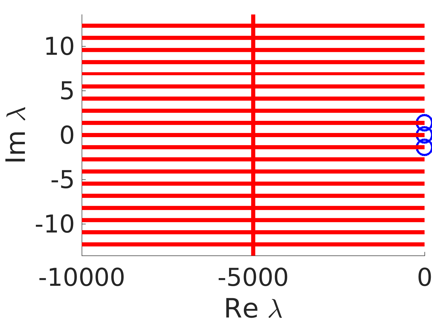
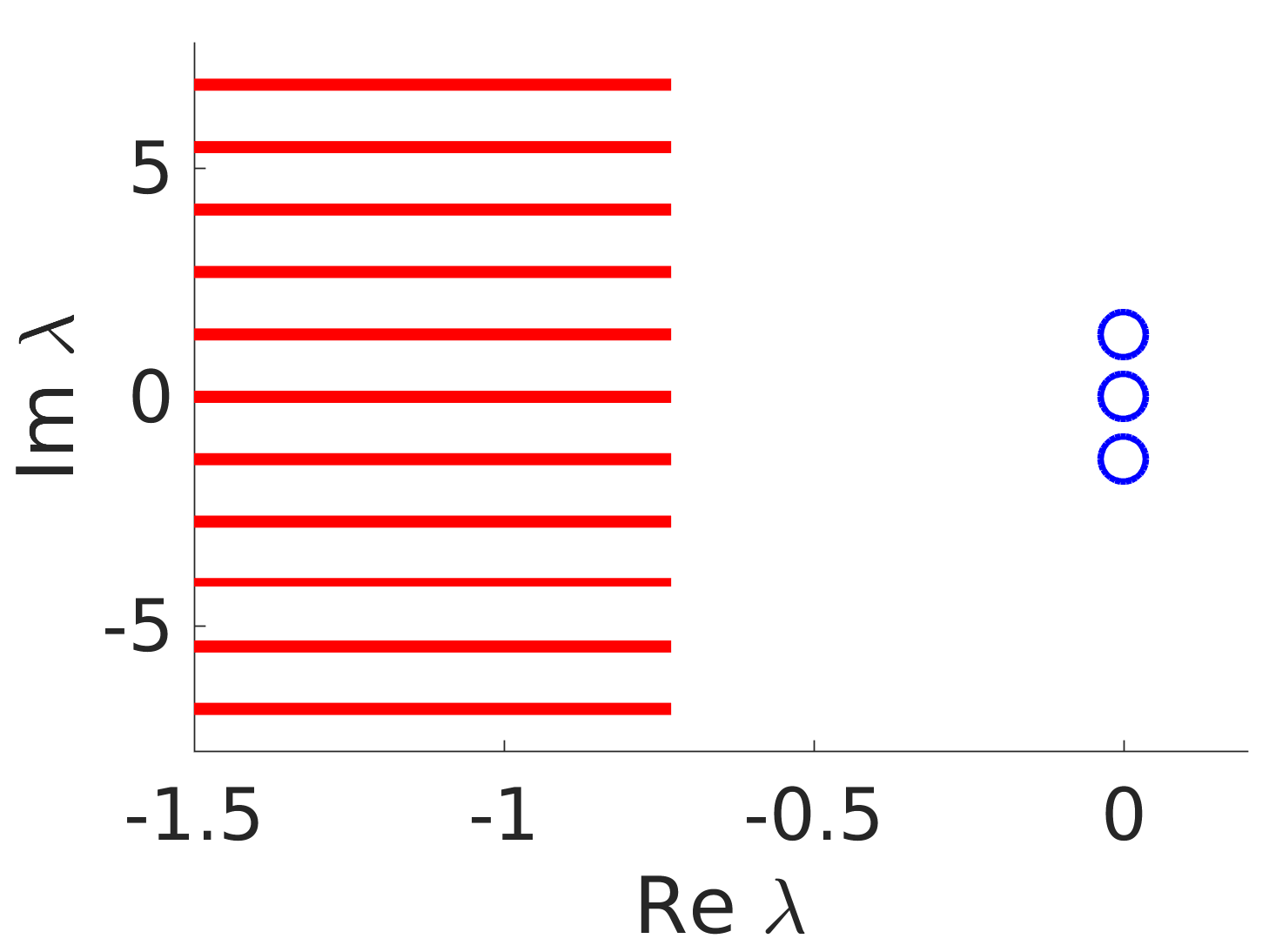
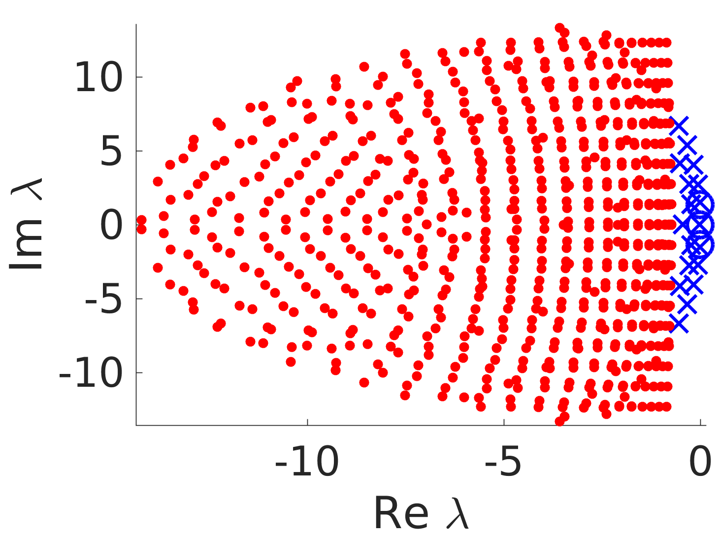
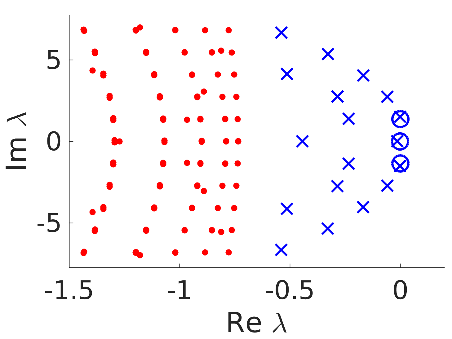
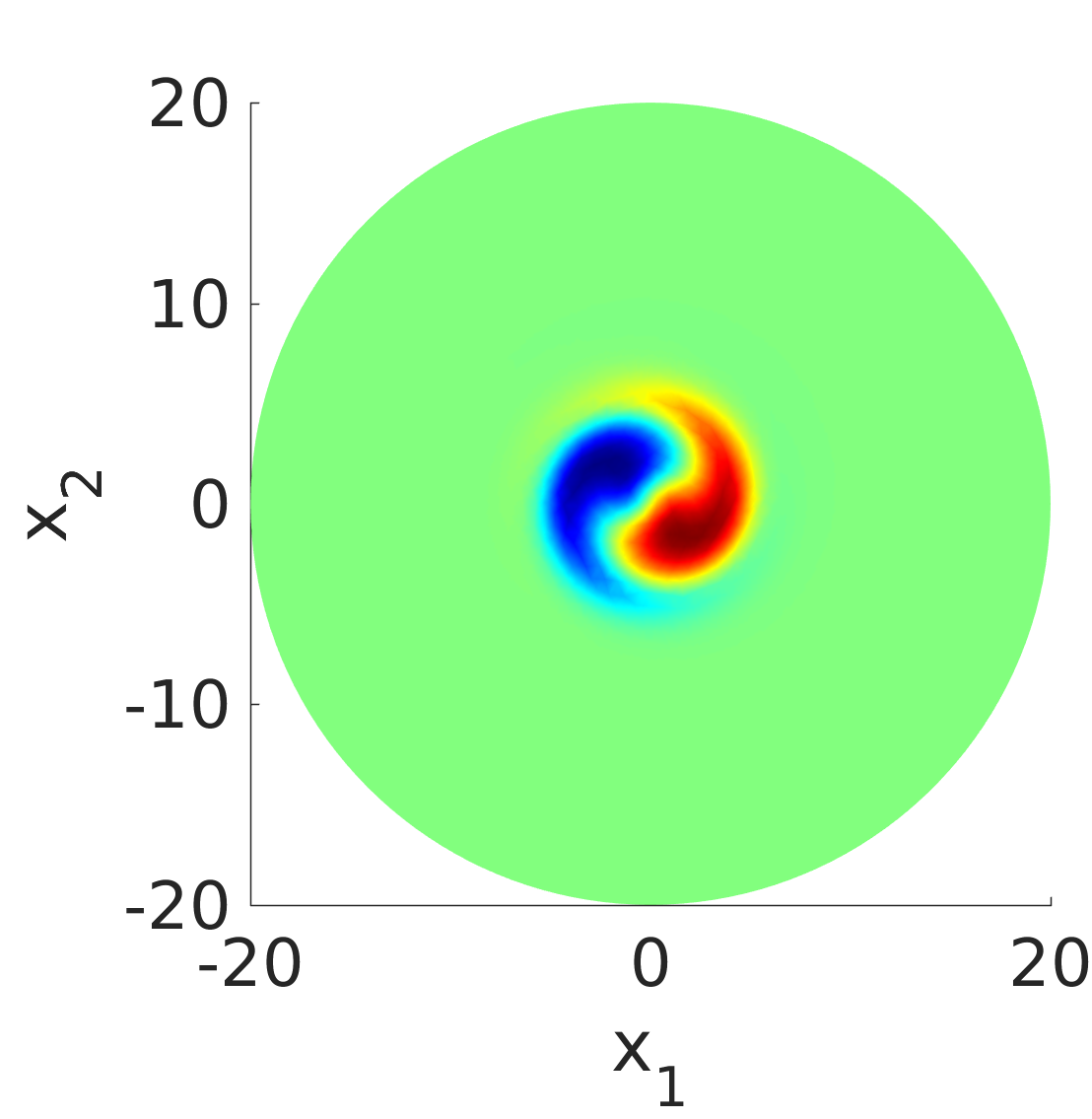
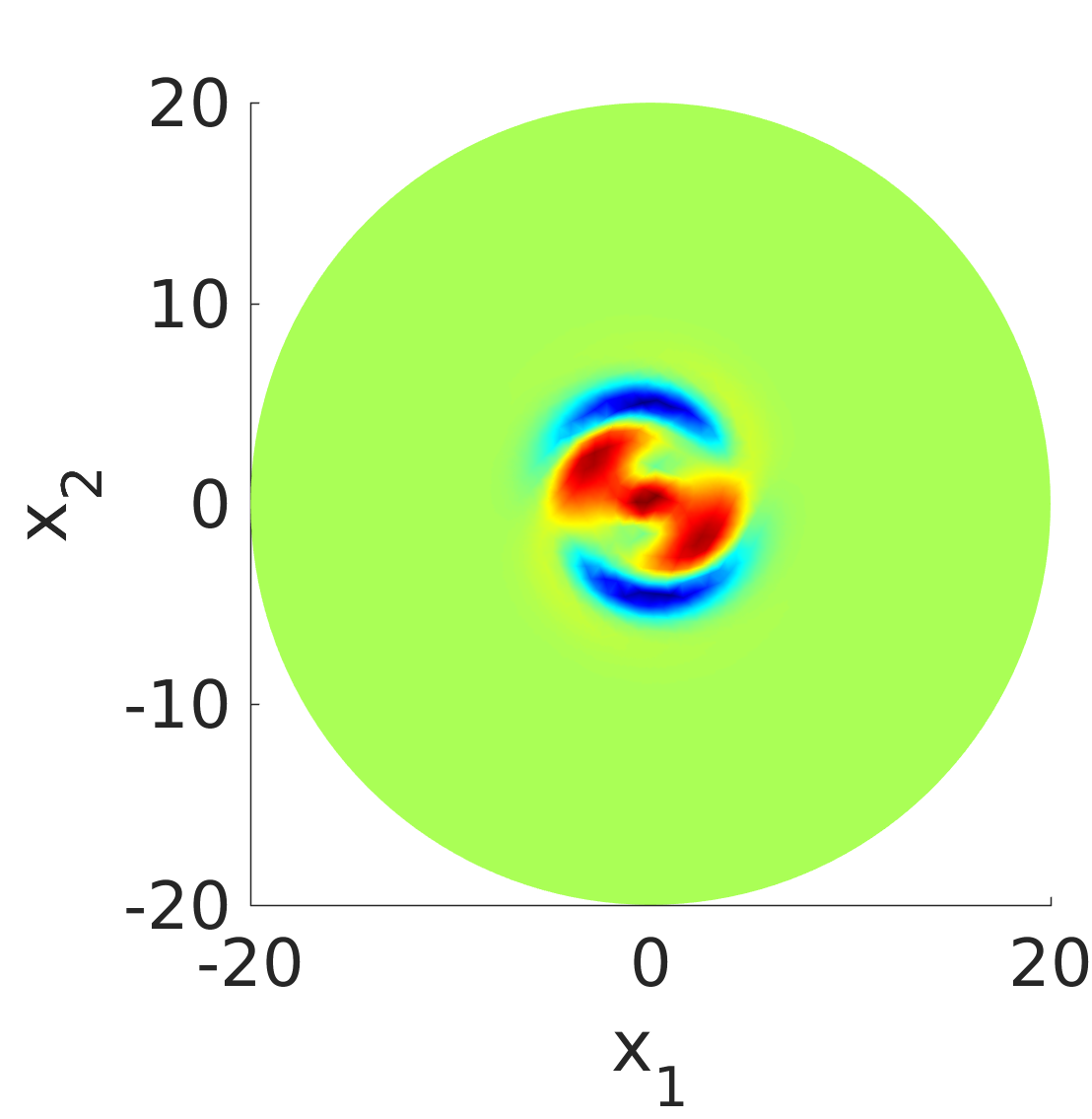
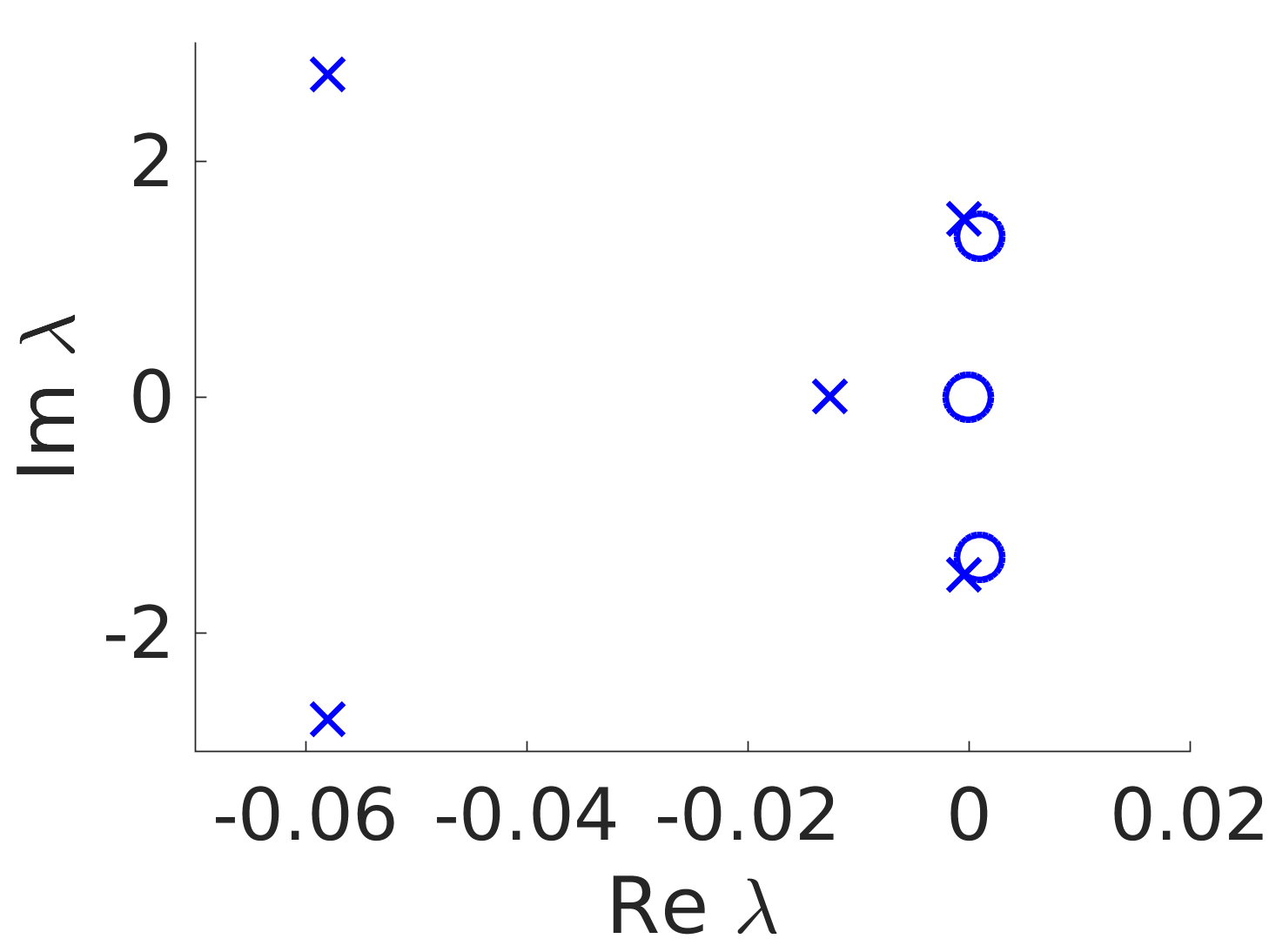
Figure 3.4(a) and (b) shows two different views for the part of the spectrum of the spinning solitons which is guaranteed by Proposition 3.3 and 3.2. It is subdivided into the symmetry set $\sigma_{\mathrm{sym}}(\mathcal{P})$ (blue circle), which is determined by Proposition 3.2 and belongs to the point spectrum $\sigma_{\mathrm{pt}}(\mathcal{P})$, and the dispersion set $\sigma_{\mathrm{disp}}(\mathcal{P})$ (red lines), which is determined by Proposition 3.3 and belongs to the essential spectrum $\sigma_{\mathrm{ess}}(\mathcal{P})$. In general, there may be further essential spectrum in $\sigma_{\mathrm{ess}}(\mathcal{P})\setminus\sigma_{\mathrm{disp}}(\mathcal{P})$ and further isolated eigenvalues in $\sigma_{\mathrm{pt}}(\mathcal{P})\setminus\sigma_{\mathrm{sym}}(\mathcal{P})$. In fact, for the spinning solitons of the cubic-quintic Ginzburg-Landau wave equation we find $18$ extra eigenvalues with negative real parts ($8$ complex conjugate pairs and $2$ purely real eigenvalues), cf. Figure 3.4(c),(d). These Figures show two different views for the numerical spectrum of the cubic-quintic Ginzburg-Landau wave equation on the ball $B_{R}(0)$ with radius $R=20$ equipped with homogeneous Neumann boundary conditions. They consist of the approximations of the point spectrum subdivided into the symmetry set (blue circle) and additional isolated eigenvalues (blue cross sign), and of the essential spectrum (red dots). Three of these isolated eigenvalues are very close to the imaginary axis, see Figure 3.5(c). Therefore, the spinning solitons seem to be only weakly stable. Finally, the approximated eigenfunctions belonging to the eigenvalues $\lambda\approx 0$ and $\lambda\approx+i\sigma$ are shown in Figure 3.5(a) and (b). In particular, Figure 3.5(a) is an approximation of the rotational term $\langle Sx,\nabla v_{\star}(x)\rangle$.

Figure 3.5. Eigenfunctions of the cubic-quintic Ginzburg-Landau wave equation for parameters (3.12) belonging to the isolated eigenvalues $\lambda_{1}\approx 0$ (a) and $\lambda_{2}\approx i\sigma$ (b) and a zoom into the spectrum from Fig.3.4(c) in (c).

Acknowledgement. We gratefully acknowledge financial support by the Deutsche Forschungsgemeinschaft (DFG) through CRC 701 and CRC 1173.

References

- [1] I. Alonso-Mallo and N. Reguera. Numerical detection and generation of solitary waves for a nonlinear wave equation. Wave Motion, 56:137–146, 2015.
- [2] W.-J. Beyn and J. Lorenz. Nonlinear stability of rotating patterns. Dyn. Partial Differ. Equ., 5(4):349–400, 2008.
- [3] W.-J. Beyn and D. Otten. Fredholm Properties and -Spectra of Localized Rotating Waves in Parabolic Systems. Preprint to appear, 2016.
- [4] W.-J. Beyn and D. Otten. Spatial decay of rotating waves in reaction diffusion systems. Dyn. Partial Differ. Equ., 13(3):191–240, 2016.
- [5] W.-J. Beyn, D. Otten, and J. Rottmann-Matthes. Stability and computation of dynamic patterns in PDEs. In Current Challenges in Stability Issues for Numerical Differential Equations, Lecture Notes in Mathematics, pages 89–172. Springer International Publishing, 2014.
- [6] W.-J. Beyn, D. Otten, and J. Rottmann-Matthes. Computation and stability of traveling waves in second order equations. Preprint, http://arxiv.org/abs/1606.08844, 2016 (submitted).
- [7] W.-J. Beyn, S. Selle, and V. Thümmler. Freezing multipulses and multifronts. SIAM J. Appl. Dyn. Syst., 7(2):577–608, 2008.
- [8] W.-J. Beyn and V. Thümmler. Freezing solutions of equivariant evolution equations. SIAM J. Appl. Dyn. Syst., 3(2):85–116 (electronic), 2004.
- [9] A. M. Bloch and A. Iserles. Commutators of skew-symmetric matrices. Internat. J. Bifur. Chaos Appl. Sci. Engrg., 15(3):793–801, 2005.
- [10] H. Brunner, H. Li, and X. Wu. Numerical solution of blow-up problems for nonlinear wave equations on unbounded domains. Commun. Comput. Phys., 14:574–598, 2013.
- [11] B. Fiedler and A. Scheel. Spatio-temporal dynamics of reaction-diffusion patterns. In Trends in nonlinear analysis, pages 23–152. Springer, Berlin, 2003.
- [12] T. Gallay and R. Joly. Global stability of travelling fronts for a damped wave equation with bistable nonlinearity. Ann. Sci. Éc. Norm. Supér. (4), 42(1):103–140, 2009.
- [13] T. Gallay and G. Raugel. Stability of travelling waves for a damped hyperbolic equation. Z. Angew. Math. Phys., 48(3):451–479, 1997.
- [14] R. Glowinski and A. Quaini. On the numerical solution to a nonlinear wave equation associated with the first Painlevé equation: an operator splitting approach. In Partial differential equations: theory, control and approximation, pages 243–264. Springer, Dordrecht, 2014.
- [15] G. Metafune. -spectrum of Ornstein-Uhlenbeck operators. Ann. Scuola Norm. Sup. Pisa Cl. Sci. (4), 30(1):97–124, 2001.
- [16] G. Metafune, D. Pallara, and E. Priola. Spectrum of Ornstein-Uhlenbeck operators in spaces with respect to invariant measures. J. Funct. Anal., 196(1):40–60, 2002.
- [17] D. Otten. Spatial decay and spectral properties of rotating waves in parabolic systems. PhD thesis, Bielefeld University, 2014, www.math.uni-bielefeld.de/~dotten/files/diss/Diss_DennyOtte%n.pdf. Shaker Verlag, Aachen.
- [18] D. Otten. Exponentially weighted resolvent estimates for complex Ornstein-Uhlenbeck systems. J. Evol. Equ., 15(4):753–799, 2015.
- [19] M. A. Rincon and N. P. Quintino. Numerical analysis and simulation of nonlinear wave equation. J. Comput. Appl. Math., 296:247–264, 2016.
- [20] J. Rottmann-Matthes. Computation and stability of patterns in hyperbolic-parabolic Systems. PhD thesis, Bielefeld University, 2010.
- [21] J. Rottmann-Matthes. Stability and freezing of nonlinear waves in first order hyperbolic PDEs. Journal of Dynamics and Differential Equations, 24(2):341–367, 2012.
- [22] J. Rottmann-Matthes. Stability and freezing of waves in non-linear hyperbolic???parabolic systems. IMA Journal of Applied Mathematics, 77(3):420–429, 2012.
- [23] J. Rottmann-Matthes. Stability of parabolic-hyperbolic traveling waves. Dyn. Partial Differ. Equ., 9(1):29–62, 2012.
- [24] C. W. Rowley, I. G. Kevrekidis, J. E. Marsden, and K. Lust. Reduction and reconstruction for self-similar dynamical systems. Nonlinearity, 16(4):1257–1275, 2003.
- [25] B. Sandstede. Stability of travelling waves. In Handbook of dynamical systems, Vol. 2, pages 983–1055. North-Holland, Amsterdam, 2002.
- [26] V. Thümmler. Numerical bifurcation analysis of relative equilibria with Femlab. in Proceedings of the COMSOL Users Conference (Comsol Anwenderkonferenz), Frankfurt, Femlab GmbH, Goettingen, Germany, 2006.
- [27] V. Thümmler. The effect of freezing and discretization to the asymptotic stability of relative equilibria. J. Dynam. Differential Equations, 20(2):425–477, 2008.
- [28] V. Thümmler. Numerical approximation of relative equilibria for equivariant PDEs. SIAM J. Numer. Anal., 46(6):2978–3005, 2008.