Fast Multipole Method based filtering of non-uniformly sampled data

Abstract

Non-uniform fast Fourier Transform (NUFFT) and inverse NUFFT (INUFFT) algorithms, based on the Fast Multipole Method (FMM) are developed and tested. Our algorithms are based on a novel factorization of the FFT kernel, and are implemented with attention to data structures and error analysis.

Note: This unpublished manuscript was available on our web pages and has been referred to by others in the literature. To provide a proper archival reference we are placing it on arXiv.

1 Introduction

Most signal processing involves the manipulation of various transforms of discretely sampled data, especially of Fourier transforms. Direct computation of a transform of $N$ data samples requires $ON^{2})$ operations. For band-limited data that is sampled at equispaced locations, the rediscovery in 1965 by [1] of an $O(N\log N)$ algorithm, the fast Fourier transform, lead to a revolution. It is difficult to overstate its impact on science and industry.

Unfortunately, many applications require transforms between nonuniformly sampled data, and recently there has been much interest in this area, especially for various inverse scattering calculations and as a component of the computation of other transforms, e.g., on the sphere. The goal is to achieve fast ($o\left(N^{2}\right))$ bandwidth-preserving transforms of data. Due to reasons of space we do not discuss these here, and refer the reader to a recent review of NUFFTs [3]. We focus instead on extensions of the work of Dutt &Rokhlin [2], who used the Fast Multipole Method (FMM) to achieve a NUFFT of asymptotic complexity $O(N(\log N-\log\epsilon))$, where $\epsilon$ is the specified error.

Here, we too apply the FMM to obtain NUFFTs and INUFFTs. The major difference is in the factorization we used for the kernel function, and our efficient implementation using data structures, supported by tests for $N$ $\simeq 10^{6}$. We show that for machine precision, the complexity of the FMM-based NUFFT and INUFFT is $O(N)$. We present theoretical and computational analyses of error bounds and optimal settings for the FMM.

2 Formulation & Solution

We consider the following two problems: i) a 2$\pi$-periodic complex-valued band-limited function $f(x)$ is sampled at $N$ equispaced points, $x_{k}=2\pi k/N,$ $k=0,...,N-1,$ so $f_{k}=f(x_{k})$;  find $g_{j}=f(y_{j}),$ $j=0,...,M-1$, where $y_{j}\in\left[0,2\pi\right)$ are non-equispaced points with specified accuracy $\epsilon;$ ii) the same function is given at $M$ non-uniform samples $g_{j},$ $j=0,...,M-1$ on a non-uniform grid $\left\{y_{j}\right\}$; determine $f_{k}$, $k=0,...,N-1$,  on a uniform grid $\left\{x_{k}\right\}.$ $N$ determines the bandwidth of $f$, since

$$f(x)=\sum_{n=0}^{N-1}c_{n}e^{inx},\quad c_{n}=\frac{1}{N}\sum_{k=0}^{N-1}f_{k}e^{-inx_{k}},$$ (1)

where $c_{n}$ are the Fourier coefficients. The forward DFT is the transform $\left\{f_{k}\right\}\rightarrow\left\{c_{n}\right\},$ and the IDFT is transform $\left\{c_{n}\right\}\rightarrow\left\{f_{k}\right\}$ .  For $N=2^{L},$ the transforms $\left\{f_{k}\right\}\rightleftarrows\left\{c_{n}\right\}$ can be done in $O(N\log N)$ operations using the FFT. Therefore, if interpolation problems $\left\{f_{k}\right\}\rightleftarrows\left\{g_{j}\right\}$ can be solved with the same efficiency, NUFFT and INUFFT, which are transforms $\left\{c_{n}\right\}\rightleftarrows$ $\left\{g_{j}\right\}$ will be available. Eq. (1) can be written as

$$\left\{g_{j}\right\}=\left\{K_{jk}\right\}\left\{f_{k}\right\},\quad K_{jk}=\frac{1}{N}\sum_{n=0}^{N-1}e^{-inx_{k}}e^{iny_{j}},$$ (2)

where $j=0,...,M-1;$ $k=0,...,N-1.$ It relates the vectors $\left\{g_{j}\right\}$ and $\left\{f_{k}\right\}$ via the sampled kernel matrix $\left\{K_{jk}\right\}$. The sum (2) is a geometric progression, and can be simplified as

$$\!\!\!\!\!\!\!\!\!\!K_{jk}=\frac{e^{iNy_{j}}-1}{e^{i\left(y-x_{k}\right)}-1}=F_{j}G\left(y_{j}-x_{k}\right),$$ (3a)

$$\!\!\!\!\!\!\!\!\!\!F_{j}=\frac{e^{iNy_{j}}-1}{N},G\left(t\right)=\frac{1}{e^{it}-1}=-\frac{1+i\cot\left(t/2\right)}{2}.$$ (3b)

This decomposition was derived in [2]. It can be thought of as a modulation of a fast oscillating function $$F(y) G\left(t\right) F(y_{j}) O(M) G\left(t\right) \left\{g_{j}\right\}\rightarrow\left\{f_{k}\right\}$$ by a slowly changing amplitude function amplitude. Evaluation of costs , while evaluation of can be done approximately by fast methods, such as the FMM. The transform can be reduced similarly. It leads to

$$\left\{f_{k}\right\}=\left\{L_{kj}\right\}\left\{g_{j}\right\},~{}~{}L_{kj}=C_{k}G\left(x_{k}-y_{j}\right)D_{j},$$ (4)

where $j=0,...,M-1;$ $k=0,...,N-1$. The kernel $L$ is decomposed as in [2], where $G\left(t\right)$ is given by Eq. (3b); and $C_{k}$ and $D_{j}$ are coefficients depending on $\left\{x_{k}\right\}$ and $\left\{y_{j}\right\}$

$$\!\!\!\!\!\!C_{k}=\left(-1\right)^{k}\!\prod_{j=0}^{N-1}\sin\frac{x_{k}-y_{j}}{2},\quad D_{j}\!=\!\frac{2ie^{-iNy_{j}/2}}{\prod_{\begin{subarray}{c}k=0,\\ k\neq j\end{subarray}}^{N-1}\sin\frac{y_{j}-y_{k}}{2}}.$$ (5)

These coefficients can be preccomputed using the FMM. So both the forward and inverse problems can be reduced to multiplication of a matrix generated by kernel $G\left(t\right)$ by some input vector. This is the problem which is in the focus of the present paper.

2.1 Multilevel FMM

For computation of the matrix-vector product $\left\{G\left(y_{j}-x_{k}\right)\right\}\left\{f_{k}\right\}$ we use the Multilevel FMM (MLFMM), a description of which can be found elsewhere [6, 4]. Note that $\left\{x_{k}\right\}$ or $\left\{y_{j}\right\}$ need not be equispaced for the FMM. Both (2) and (4) use the same algorithm with source and target sets $\left\{x_{k}\right\}$ & $\left\{y_{j}\right\}$ exchanged.

Space Partitioning: The kernel $\cot\frac{y_{j}-x_{k}}{2}$ is a $2\pi$-periodic function. We can thus make transforms $\widetilde{x}_{k}=x_{k}+2\pi n,$ $n=0,\pm 1,...$, which do not change the function, and keep $y_{j}-$ $\widetilde{x}_{k}$ in $-\pi\leqslant y_{j}-$ $\widetilde{x}_{k}\leqslant\pi;,$ i.e., $y_{j}$ and $x_{k}$ are points on a unit circle. Then $x_{k}$ and $\widetilde{x}_{k}$ are identical (see Fig. 1).

Figure 1: On the left locations of the source, $\left\{x_{k}\right\},$ and target, $\left\{y_{j}\right\},$ points on the unit circle are shown. The circle is subdivided at level 2 into 4 arcs. In the center the behavior of the kernel function $\cot(t/2)$ is shown. At the right the hierarchical space partitioning employed in the MLFMM is illustrated. Arrows show the hierarchical parent-children relations in the binary tree.

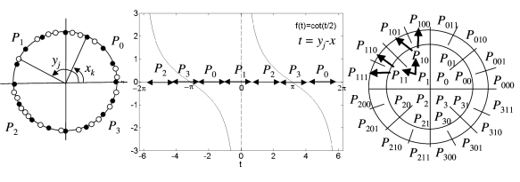
In the case of circular topology, hierarchical space partitioning with a binary tree with $l_{\max}$ levels, leads to a division of the circle by $2^{l}$ equal arcs. In this hierarchy, parent-children relations are defined as in a binary tree, but the concept of neighbors and neighborhoods is modified. At level 2 we subdivide $\left[0,2\pi\right)$ into 4 pieces: $P_{0}:\left[0,\pi/2\right),$ $P_{1}:\left[\pi/2,\pi\right),$ $P_{2}:\left[\pi,3\pi/2\right),$ $P_{3}:\left[3\pi/2,2\pi\right),$ where $P_{2}$ and $P_{0}$ are neighbors of $P_{3}$ and they together form a neighborhood of $P_{3},$ which we denote as $\Omega_{1}(P_{3}).$ We also denote $P_{1}$ as $\Omega_{2}(P_{3}),$ i.e. the piece outside the neighborhood of $P_{3}$.

2.2 Kernel Expansions:

Level $l=2$ requires special consideration. Here we separate the sum over all the sources as

$$\!\!\!\!\!h\left(y_{j}\right)=\!\!\sum_{x_{k}\in\Omega_{1}(P_{n})}f_{k}\cot\frac{y_{j}-x_{k}}{2}+\!\!\sum_{x_{k}\in\Omega_{2}(P_{n})}f_{k}\cot\frac{y_{j}-x_{k}}{2},$$ (6)

$y_{j}\in P_{n};$ $n=0,...,3.$ The first sum can be computed using:

$$\cot\frac{t}{2}=\frac{2}{t}-2\sum_{m=1}^{\infty}\frac{\left|B_{2m}\right|}{\left(2m\right)!}t^{2m-1},\quad\left|t\right|<2\pi,$$ (7)

where $B_{m}$ are the Bernoulli numbers [5]. When applied here, we note that for $x_{k}\in\Omega_{1}(P_{n})$ we have $-\pi\leqslant y_{j}-\widetilde{x}_{k}\leqslant\pi,$ so for $t$ $=y_{j}-\widetilde{x}_{k}$ we have $\left|t\right|\leqslant\pi.$ This provides fast convergence in Eq. (7), which otherwise blows up as $y_{j}-x_{k}\rightarrow\pm 2\pi.$

For the second sum, we introduce $t=y_{j}-\widehat{x}_{k}$, where $\widehat{x}_{k}=x_{k}\pm\pi$ is a point opposite $x_{k}$. We have

$$\!\!\cot\frac{y_{j}-x_{k}}{2}\!=\!-\tan\frac{t}{2}\!=\!-2\sum_{m=1}^{\infty}\frac{\left(2^{2m}-1\right)\left|B_{2m}\right|}{\left(2m\right)!}t^{2m-1},$$ (8)

$\left|t\right|<\pi.$ Note that as $t\rightarrow\pm\pi$ the series blows up. However, since $x_{k}\in\Omega_{2}(P_{n})$ we have $\widehat{x}_{k}\in P_{n}.$ Due to both $y_{j}$ and $\widehat{x}_{k}$ belong to the same $P_{n}$, whose length is $\pi/2,$ we have $-\pi/2\leqslant y_{j}-\widehat{x}_{k}\leqslant\pi/2,$ or $\left|t\right|\leqslant\pi/2.$ This provides a fast convergence of the sum.

There are thus two parts to the kernel function $\cot\left(t/2\right):$ singular ($2/t)$, and regular. Fast summation with the singular kernel can be performed using the MLFMM, while the regular part can be truncated and factorized for all points in the respective neighborhoods at level 2. The MLFMM for kernel $1/t$ has been well studied, optimized, and error bounds are established [4]. We just modified our software in [4] with a circular data structure.

2.3 Truncation Errors:

Consider the truncation error for sum (7) when $q$ first terms of the expansion are used to approximate the infinite sum. We note that the Bernoulli numbers satisfy [5]

$$\left|B_{2m}\right|<\frac{2\left(2m\right)!}{\left(2\pi\right)^{2m}}\frac{1}{1-2^{1-2m}},\quad m=1,2,...$$ (9)

This shows that the truncated part of the series can be majorated by the geometric progression. Using $\left|t\right|\leqslant\pi,$ the error bound is

$$\left|\epsilon_{q}^{(1)}\right|\!=\left|\!\sum_{m=q+1}^{\infty}\frac{\left|B_{2m}\right|t^{2m-1}}{\left(2m\right)!}\right|<\frac{2^{1-2q}}{3\pi\left(1-2^{-2q-1}\right)}=\epsilon_{q}.$$ (10)

The truncation error, $\epsilon_{q}^{(2)},$ in (8) can be bounded similarly, using $\left|t\right|\leqslant\pi/2$: $\left|\epsilon_{q}^{(2)}\right|<\!2\epsilon_{q}.$ The estimates are for a single source-evaluation pair. For $3N/4$ sources located in the neighborhood of point $y_{j}$, and $N/4$ outside it, the total maximum absolute error in computation of $g_{j}$ (with $\left|f_{k}\right|\leqslant 1)$ is

$$\!\!\!\!\!\!\left|\epsilon_{q}^{reg}\right|\!=\!\left|\sum_{k=0}^{N-1}\left(K_{jk}-K_{jk}^{(q)}\right)f_{k}\!\right|<\frac{2}{N}\left(\frac{3N\epsilon_{q}}{4}+\frac{2N\epsilon_{q}}{4}\right)=\frac{5\epsilon_{q}}{2}.$$

The error of the MLFMM with kernel $1/t$ has been estimated in [4]. This result applied to our case in a computational domain of size $3\pi/2,$ and for $3N/4$ sources is

$$\left|\epsilon_{p}^{MLFMM}\right|<\frac{5}{\pi}\cdot 2^{l_{\max}}3^{-p},$$ (11)

where $l_{\max}$ is the maximum level of space subdivision and $p$ is the truncation number used in the MLFMM. Therefore the total truncation error for the present method can be estimated as

$$\epsilon\lesssim\frac{5}{3\pi}\left(4^{-q}+2^{l_{\max}}3^{1-p}\right).$$ (12)

By requiring that the error in the singular and regular parts be the same in (12) we relate  $p$ and $q$, and obtain a combined bound as

$$q\gtrsim\frac{1}{2}\log_{2}\frac{3\pi}{10\epsilon},\quad p\gtrsim\log_{3}\frac{3\pi}{10\epsilon}+\frac{l_{\max}}{\log_{2}3}+1.$$ (13)

2.4 Complexity and Optimizations:

For fast computations of the products involving $q$-truncated sums (7) and (8) we factorize powers $t^{2m-1}$ using the Newton binomial expansion near the center, $x_{c}^{(n)}$, of the segment $P_{n}$ containing $y_{j}.$ Substituting this expansion into Eqs (7) and (8) and further into Eq. (6), we obtain after changing the order of summation:

$$h\left(y_{j}\right)=2\sum_{x_{k}\in\Omega_{1}(P_{n})}\frac{f_{k}}{y_{j}-\widetilde{x}_{k}}-\sum_{l=0}^{2q-1}\frac{d_{l}}{l!}\left(y_{j}-x_{c}^{(n)}\right)^{l},$$ (14)

$$d_{l}=\sum_{m=\left[l/2\right]+1}^{q}\frac{\left|B_{2m}\right|}{m}\left[\alpha_{2m-l-1}^{(1)}+\left(2^{2m}-1\right)\alpha_{2m-l-1}^{(2)}\right],$$

$$\alpha_{l}^{(s)}=\frac{1}{l!}\sum_{x_{k}\in\Omega_{s}(P_{n})}f_{k}\left(x_{c}^{(n)}-\widetilde{x}_{k}\right)^{l},\quad s=1,2.$$

For $2q\ll\min(N,M)$ the second sum in Eq. (14) is $O\left(2q\left(N+M\right)\right).$ For the complexity of the MLFMM in the present case we have [4]

$$C_{FMM}=O\left(p\left(N+M\right)+\frac{3NM}{2^{l_{\max}}}+\frac{6P}{2^{-l_{\max}}}\right),$$ (15)

where $P(p)$ is the cost of a single translation for truncation $p$ .

The total cost of the fast Fourier interpolation algorithm (FFIA) can be estimated, and minimized by selection of $l_{\max}$ for given error (12). A simplified estimate assuming that $p$ and $q$ change slower than $2^{l_{\max}},$ yields

$$l_{\max}^{(opt)}\sim\frac{1}{2}\log_{2}\frac{NM}{2P},$$ (16)

and the total complexity of the optimized algorithm will be

$$C_{FFIA}^{(opt)}=O\left(\left(N+M\right)\left(p+2q\right)+6\left[2NMP(p)\right]^{1/2}\right).$$ (17)

For $N\sim M,$ this yields $C_{FFIA}^{(opt)}=O\left(N\left(\log N+\log\epsilon^{-1}\right)\right)$.

3 Numerical study

The FFIA was implemented and tested on a 933 MHz Pentium III Xeon PC with 1GB RAM. in complex double precision. Tests were performed for $M$ $=N=2^{L}$ varying in $2^{3}-2^{20}$ for various $l_{\max},p,$ and $q$. In all cases, $y_{j},$ $j=0,...,M-1$ were randomly distributed in $\left[0,2\pi\right)$ for the transform $\left\{f_{k}\right\}\rightarrow\left\{g_{j}\right\}$ and were within 10% perturbation near the centers $\left\{x_{k}\right\}$ for the transform $\left\{g_{j}\right\}\rightarrow\left\{f_{k}\right\}.$ We found that the errors for the latter depend substantially on the distribution of $\left\{y_{j}\right\},$ while for $\left\{f_{k}\right\}\rightarrow\left\{g_{j}\right\}$ there was no such dependence. We thus focused on the transform $\left\{f_{k}\right\}\rightarrow\left\{g_{j}\right\},$ since the error analysis for the other case should be combined with a more rigorous study of non-uniformity errors and errors in computation of coefficients (5).

Figure 2: Dependences of $\epsilon_{a}$, for the FFIA solution on the prescribed $\epsilon$ for various $N$, indicated near the curves.

3.1 Error analysis

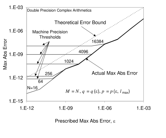
We performed several error tests to ensure that the algorithm worked properly and results were consistent with theory. First, we took the analytical solution $f\left(x\right)\equiv 1,.$ and varied $l_{\max}$ from $3$ to $L=\log_{2}N$, and prescribed $\epsilon=10^{-12},...,10^{-3};$ $q$ and $p$ were found from (13). Results of the tests are in Fig. 2. The actual error was measured as $\epsilon_{a}=\max_{j}\left|g_{j}-1\right|$ and depends on $N,l_{\max},\epsilon.$ We observed that $\epsilon_{a}$ just slightly depends on $l_{\max}$, consistent with (12). Another theoretical prediction provided by Eq. (12) is that the error should not depend on $N$. Fig. 2 shows this for $\epsilon\gg\epsilon_{th}(N),$ where $\epsilon_{th}(N)$ is a threshold error, which we refer as “machine precision error”; $\epsilon_{a}$ was much smaller than $\epsilon$.

Figure 3: Dependence of the CPU time on $l_{\max}$ in the MLFMM for prescribed $\epsilon=10^{-6}$ for different $N$. The small numbers near the right end of the curves show $\epsilon_{a}$

To validate that $\epsilon_{th}$ is really related to the machine precision arithmetic, we performed a test, when $\left\{g_{j}\right\}$ was computed by the “exact” straightforward method, i.e. by multiplication of matrix $\left\{K_{jk}\right\}$ computed using Eq. (3a) by vector $\left\{f_{k}\right\}$. The results of this test yield dependence $\epsilon(N),$ which is consistent with $\epsilon_{th}(N)$ obtained in experiments using the “approximate” fast method. We also compared the maximum absolute difference between the results obtained using the straightforward method and the FFIA for constant and random $f_{k}\in\left[0,1\right]$. In both cases for $\epsilon=10^{-12}$ this error was smaller than $\epsilon_{th}(N).$

We can thus conclude that the theoretical error or machine precision bound the FFIA error. It makes no sense to specify an error below the precision, and this provides a result on the asymptotic complexity of the MLFMM. Indeed, estimation $C_{FFIA}^{(opt)}=O(N\log N)$ does not take into account the growth of $\epsilon_{th}(N)$ with $N$ due to roundoff errors, while assumes that computations are done with arbitrary precision. However, this happens only for $\epsilon\gg\epsilon_{th}(N)$. If the computational task is formulated as “solve the problem with machine precision” then the complexity will be $O(N).$

3.2 Optimization:

We conducted optimization tests in two basic settings for error control. The first case we considered is minimization of the CPU time for fixed prescribed error $\epsilon\geqslant\epsilon_{th}(N)$. The second case is minimization of the CPU time for computations with maximum available machine precision. In the first case the range of $N$ was limited by condition $\epsilon\geqslant\epsilon_{th}(N)$ and in the second case $N$ was limited by machine resources available.

Figure 4: Dependences of the CPU time on $N,$ for the straightforward method (dark circles), and present method (FFIA) with prescribed accuracy (dark diamonds and triangles) and with the machine precision (light squares). The light circles show CPU time for setting the data structure. The dark squares show the CPU time required for FFT on the same machine.

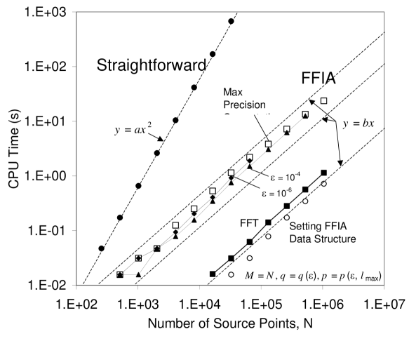
Fig. 3 illustrates dependence of the CPU time on $l_{\max}$ at fixed $\epsilon=10^{-6}$ and different $N$. Truncation numbers $q$ and $p$ were selected using (13). The actual error of computations $\epsilon_{a}$ was estimated by comparison with analytical solution, $f\equiv 1$ and shown on Fig. 3.

Figure 5: Truncation numbers, $q$ (circles) and $p$ (squares), vs $N$. Dark circles and squares show dependence of computation with fixed $\epsilon$. Light circles and squares show the threshold dependences $q_{th}\left(N\right),$ $p_{th}\left(N\right)$ Obtained using Eq. (13) for $\epsilon=\epsilon_{th}\left(N\right)$.

All curves on Fig. 3 clearly show that there exist an optimum maximum level of the space subdivision, $l_{\max}^{(opt)},$ for the MLFMM. The CPU time for computations with $l_{\max}=l_{\max}^{(opt)}$ and non-optimized $l_{\max}$ can differ substantially. An empirical correlation is $l_{\max}^{(opt)}=\log_{2}N-l_{\ast}(\epsilon),$ where $l_{\ast}(\epsilon)$ depends on the algorithm implementation (in our case $l_{\ast}(\epsilon)=5$, see Fig. 3).

In the second case we imposed experimentally measured machine precision threshold $\epsilon_{th}(N)$ as the prescribed accuracy $\epsilon.$ In this case we found that the same dependence $l_{\max}^{(opt)}(N)$ describes $l_{\max}^{(opt)}\left(L\right)$ well. We also noted that the actual error of computations $\epsilon_{a}$ was equal to $\epsilon_{th}(N)$ for $\epsilon=\epsilon_{th}(N).$

3.3 Speed of Computations:

To evaluate the algorithm we measured CPU time for the straightforward method, and the optimized FFIA for computations with fixed $\epsilon\geqslant\epsilon_{th}(N)$ and machine precision, $\epsilon=\epsilon_{th}(N).$ It is noticeable that the MLFMM procedures consist of two steps: setting the data structure, the step which needs to be performed when the target data set $\left\{y_{j}\right\}$ changes, and evaluation, which is executed each time the input $\left\{f_{k}\right\}$ changes. Fig. 4 shows that the computational cost for setting the data structure grows as $O(N)$ and is much smaller than the cost of the evaluation step. In case the interpolation is performed for INUFFT, an execution of the IFFT is required for the transform $\left\{c_{n}\right\}\rightarrow\left\{f_{k}\right\}$. Fig. 4 shows that the cost of this step is low compared to the FFIA evaluation step and is slightly above that of setting of the data structure.

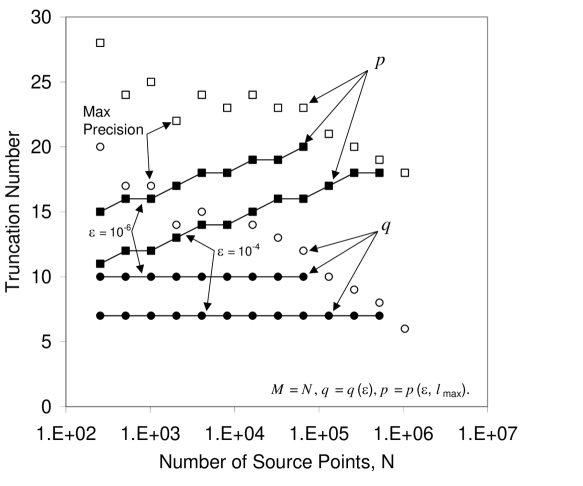
Fig. 4 also shows that the FFIA far outperforms the straightforward method even for small data sets ($N\sim 10^{2}$) and the difference gains orders of magnitude for larger $N.$ This is clear, since the straightforward method is scaled as $O(N^{2}),$ while the FFIA for maximum precision is scaled as $O(N)$. It is interesting to see that for fixed prescribed error $\epsilon,$ such as $\epsilon=10^{-6}$ and $\epsilon=10^{-4}$ shown in the figure, the CPU time required for computations deviates from the linear dependence $O(N)$ at larger $N.$ This is consistent with the estimation of the algorithm complexity $O(N\log N)$ valid for for $\epsilon\gg\epsilon_{th}(N).$ In contrast to this behavior the curve corresponding to computations with the maximum precision available, $\epsilon=\epsilon_{th}(N),$ shows deviation from the linear dependence in the opposite direction at larger $N$. The explanation of this effect comes from the error analysis provided above and also clear from Fig. 5, which illustrates the dependences of the truncation numbers on $N.$ While $q$ for fixed $\epsilon$ stays constant and $p$ increases $a+b\log N$ a different behavior of the bounding values $p_{th}$ and $q_{th}$ for maximum precision computations occurs. Both the truncation numbers, $p_{th}$ and $q_{th}$, are bounded by a global constant. Moreover, they have a tendency to decay at larger $N$ and $p_{th},q_{th}\sim a-b\log N,$ where $a$ and $b$ some constants.

4 Conclusions

We developed and tested a fast algorithm for matrix-vector multiplication with a kernel appropriate for the forward and inverse interpolation problems of band limited functions, which can be used for the forward and inverse Fourier Transforms for non-equispaced data. The algorithm far outperforms straightforward methods. Our results stay within the specified error bounds or maximum available machine accuracy. The algorithm asymptotically scales as $O(N)$ for computations with fixed maximum machine precision and as $O(N\log N+N\log\epsilon^{-1})$ otherwise. Furthermore, the current algorithm is parallelizable.

References

- [1] J.W. Cooley, J. W. Tukey. “An algorithm for the machine calculation of complex Fourier series,” Math Comp. 19, 297-301, 1965.
- [2] A. Dutt, V. Rokhlin. “Fast Fourier transforms for nonequispaced data II,” J. Comp. Harm. Anal., 2, 85-100, 1995.
- [3] D. Potts, G. Steidl, M. Tasche. “Fast Fourier transforms for nonequispaced data: A tutorial,” In: Modern Sampling Theory: Math and Applications, Birkhäuser, 253 - 274, 2001.
- [4] N.A. Gumerov, R. Duraiswami, E.A. Borovikov. “Data structures, optimal parameters, and complexity results for generalized multilevel fast multipole methods in dimensions,” UMIACS-TR-2003-28, 2003 (submitted to J. Comp. Phys.)
- [5] M. Abramowitz and I. A. Stegun (eds.). Handbook of Mathematical Functions, U. S. Government Printing Office, 1964.
- [6] L. Greengard, The Rapid Evaluation Of Potential Fields in Particle Systems, MIT Press, Cambridge, 1988.