Speeding up -body simulations of modified gravity: Chameleon screening models
Abstract
We describe and demonstrate the potential of a new and very efficient method for simulating certain classes of modified gravity theories, such as the widely studied gravity models. High resolution simulations for such models are currently very slow due to the highly nonlinear partial differential equation that needs to be solved exactly to predict the modified gravitational force. This nonlinearity is partly inherent, but is also exacerbated by the specific numerical algorithm used, which employs a variable redefinition to prevent numerical instabilities. The standard Newton-Gauss-Seidel iterative method used to tackle this problem has a poor convergence rate. Our new method not only avoids this, but also allows the discretised equation to be written in a form that is analytically solvable. We show that this new method greatly improves the performance and efficiency of simulations. For example, a test simulation with particles in a box of size is now 5 times faster than before, while a Millennium-resolution simulation for gravity is estimated to be more than 20 times faster than with the old method. Our new implementation will be particularly useful for running very high resolution, large-sized simulations which, to date, are only possible for the standard model, and also makes it feasible to run large numbers of lower resolution simulations for covariance analyses. We hope that the method will bring us to a new era for precision cosmological tests of gravity.
I Introduction
Modified gravity theories cfps2011 ; jls2016 are popular alternatives to the cosmological constant and dark energy models cst2006 to explain the observed accelerating expansion of our Universe gsetal2010 ; pretal2009 ; bbetal2011 ; rsetal2012 ; hletal2012 ; rmetal2009 . Rather than invoking a cosmological constant (), or a new energy component to drive the dynamics of the cosmos, these theories suggest that the Universe contains only normal and dark matter (which is often assumed as cold dark matter, or CDM), but the law of gravitation deviates from that prescribed by Einstein’s General Relativity (GR) on large scales, resulting in an acceleration of the expansion rate.
Since the law of gravity is universal, deviations from GR on large scales are often associated with changes in the behaviour on small scales. Any such small scale changes, however, must be vanishingly small due to the strong constraints placed by numerous local tests of gravity w2014 . Consequently, viable modified gravity theories usually have some mechanism by which such modifications are suppressed, recovering GR in dense regions like the Solar System, where those gravity tests have been carried out and their resulting constraints apply. These are commonly referred to as ‘screening mechanisms’ in the literature, and are an inherent (instead of an add-on) property which comes from the dynamics of the theory. The screening effect implies that gravity behaves differently in different environments; this environmental dependence is often reflected in strong nonlinearities in the field equations, which make both analytical and numerical studies of such theories challenging.
In most theories that are currently being investigated, the modification to GR boils down to an extra (so-called fifth) force that is mediated by a new scalar field, and screening in this context means suppression of the fifth force. In one class of such theories, this is achieved by a coupling of the scalar field to matter and a nonlinear self-interaction potential of the scalar field. With appropriate choices of the coupling and potential, the dynamics of the scalar field can ensure that, in high density regions, the fifth force it mediates decays exponentially fast with distance, or becomes extremely small in its amplitude. Chameleon theories kw2004 ; ms2007 , with gravity sf2010 (see also lb2007 ; hs2007 ; bbds2008 ) as a representative example, is an instance of the former case, while the dilaton bbds2010 and symmetron hk2010 models belong to the latter case. Amongst these models, gravity is currently the most well-studied case, and there exist numerous works investigating in detail its predictions for large-scale structure formation in the nonlinear regime. This has been made possible by the continuous development of -body simulation codes (e.g., o2008, ; olh2008, ; sloh2009, ; lz2009, ; zmlhf2010, ; lz2010, ; zlk2011, ; zlk2011b, ; lh2011, ; lzk2012, ; lkzl2012, ; lzlk2012, ; jblzk2012, ; lhkzjb2012, ). An efficient code amongst these is ecosmog ecosmog , based on the publicly available -body and hydro code ramses ramses , which makes large simulations for gravity feasible. Using the generic parametrisation for modified gravity theories bdl2011 ; bdlw2012 , ecosmog was extended to incorporate chameleon, dilaton and symmetron models bdlwz2012 ; bdlwz2013 in general. ecosmog has recently been compared with other codes developed subsequently, including mg-gadget mggadget , Isis isis and mg-enzo mgenzo and very good agreement was found between all these codes code_comparison .
There are other modified gravity theories, such as the Dvali-Gabadadze-Porrati dgp (DGP) brane-world model, in which screening is achieved by nonlinear derivative self-couplings of a scalar field. Well-studied examples include the K-mouflage kmouflage1 ; kmouflage2 and Vainshtein vainshtein mechanisms, the latter being originally studied in massive gravity theories as a means to suppress the extra helicity modes of massive gravitons so that GR is recovered in the massless limit. In addition to the nonlinear massive gravity massivegravity1 ; massivegravity2 ; cp2012 and braneworld models, the Vainshtein mechanism is also employed in general setups, such as the Galileon models nrt2009 ; dev2009 ; Galileon1 ; Galileon2 ; Galileon3 ; Galileon4 , which have been the subject of various recent studies (e.g., ck2009, ; sk2009, ; gs2010, ; dt2010, ; ndt2010, ; ags2010, ; bbd2011, ; al2012, ; al2012b, ; blbp2012, ; nrcpagb2013, ; blbp2013, ; blhlbp2014, ; fkzl2014, ; fkz2015, ; ott2013, ; wjl2013, ; zwjlw2014, ; bbll2016, ; nrabgmb2016, ).
The first two generations of modified gravity simulation codes (e.g., o2008, ; lkz2008, ; lz2010, ; zlk2011, ) were either not parallelised or had a uniform resolution across the whole simulation box, resulting in insufficient resolution and inefficiency. The current generation of codes, such as ecosmog, mg-gadget, Isis and mg-enzo, are all efficiently parallelised. These codes solve the nonlinear field equations in modified gravity on meshes (or their equivalents), and employ the adaptive mesh refinement (AMR) technique to generate ever finer meshes in high density regions to increase resolution. However, even with these parallelised codes, modified gravity simulations currently are still very slow compared to the fiducial GR case. As we shall discuss below, this is partially due to the nonlinear nature of the equations to be solved, and partly due to the specific numerical algorithms used. The greater computational cost of modified gravity simulations makes it difficult to achieve the resolution and volume attained in state-of-the-art simulations of standard gravity.
The coming decade will see a flood of high-precision observational data from a new generation of cosmological surveys, such as erosita erosita , the Dark Energy Spectroscopic Instrument (desi) desi ; desi1 ; desi2 , euclid euclid and the Large Synoptic Survey Telescope (lsst) lsst . These surveys will provide us with golden opportunities to perform cosmological tests of gravity (see ref. koyama2016, , for a recent review) and seek a better understanding of the origin of cosmic acceleration. As things stand now, it is the lack of more powerful simulation methods that limits the accuracy and size that modified gravity simulations can possibly attain, therefore preventing us from fully exploiting future observations. This has led to many attempts to speed up simulations using approximate methods (e.g., wf2015, ; bbl2015, ), or develop alternative methods to predict theoretical quantities (e.g., le2012, ; zhao2014, ; mpll2015, ; crll2016, ). These alternative methods are fast substitutes of full simulations and powerful when quickly exploring a large parameter space is the primary concern. However, simulations are nevertheless necessary to calibrate these methods or when better (e.g., %-level) accuracy is needed, as well as to study the impact of different theories of gravity on galaxy formation.
In bbl2015 , an approximate method to speed up -body simulations of Vainshtein-type models was presented and shown to reduce the overhead111Throughout this paper, the term ‘overhead’ is used to refer to the extra computational time (using the same machine and number of cores) involved in running a modified gravity simulation compared to standard gravity. For example, an overhead of 110% means that the modified gravity run requires the CPU time of a CDM simulation. of solving the modified gravity equation to the level of %, with the errors in various cosmological quantities being controlled to well under % or smaller (comparable to the discrepancies in the predictions of different modified gravity simulation codes code_comparison ). The same method, however, does not work as accurately in chameleon-type models (see Appendix A), the simulations for which are much more expensive than those for the Vainshtein-type models. Given that chameleon models are a large class of modified gravity models that are of interest to the theoretical and observational community, there is an equally urgent need for fast simulation methods for them – this is precisely the purpose of this paper.
Unlike the truncated simulation method in bbl2015 , which artificially suppresses the solver of the modified gravity equation on higher refinement levels of the AMR meshes, and instead interpolates the solution on lower (or coarser) refinement levels to find approximate solutions on higher levels, the method proposed here still solves the full modified gravity equations on all levels. The improved efficiency comes instead from a different way to discretise the equation on meshes, that makes it less nonlinear and greatly enhances the rate of convergence of the solution. The new scheme boosts the performance of the code by a factor of 5 for a simulation with a periodic box of size and particles, and by a factor of more than 20, for a higher resolution setup with a box size of and particles. The method has its own limitation, namely that the existence of analytical solutions is a particular property of Hu-Sawicki (HS) gravity – as well as a few other examples of chameleon, symmetron (see Appendix B) and dilaton – models. However, the generic nature of the HS model (in the sense that with varying parameters it covers a wide range of cosmological behaviours predicted by various other classes of models) and the lack of a preferred fundamental model make a good argument for using this model as a testbed, given that it is both impossible and unnecessary to study all chameleon-type models using simulations.
This paper will be arranged as follows. In § II we briefly describe the gravity model and the chameleon screening mechanism. In § III we recap the method currently employed in simulations and explain why it is inefficient, before describing the new method. In § IV we perform some tests as validation of this new method. Finally, we discuss and summarise in § V.
Throughout the paper we shall follow the metric convention , and set except in the expressions where appears explicitly. Greek indices run over 0, 1, 2, 3. A subscript 0 denotes the present-day value of a quantity.
II The Hu-Sawicki gravity model
In this section, we briefly review the Hu-Sawicki design (hs2007, ) of gravity, which is currently the most widely studied one in the literature.
II.1 The model
gravity is obtained by replacing the Ricci scalar in the standard Einstein-Hilbert action with an algebraic function of (see, e.g., ref. sf2010, , for a review):
| (1) |
in which is Newton’s gravitational constant, the determinant of the metric tensor and is the Lagrangian density for matter fields (including cold dark matter, baryons, radiation and neutrinos).
The inclusion of in Eq. (1) changes the Einstein equation from second order to 4th order in derivatives of the metric tensor. However, one can straightforwardly rewrite the equation into two second order ones by defining a new variable, a scalar field, . These include an equation of motion that governs the dynamics of the scalar field:
| (2) |
and a modified Einstein equation:
| (3) |
with
| (4) |
in which is the matter energy-momentum tensor, the mass density of non-relativistic matter species, the covariant derivative compatible with metric , the Laplacian operator, the Ricci tensor and the Einstein tensor.
In the nonlinear regime of structure formation, assuming the quasistatic (bhl2015, ) and weak-field approximations, Eq. (3) simplifies to a modified Poisson equation,
| (5) |
which relates the gravitational potential at a given position to the density (, where a bar denotes the cosmic mean of a quantity) and curvature () at that position.
Similarly, Eq. (2) reduces to
| (6) |
Eqs. (5) & (6) need to be solved in cosmological simulations for gravity to predict the modified gravitational force that is responsible for structure formation. It can be seen that Eq. (6) has a similar form to the Poisson equation, but is generally a nonlinear function of , and this makes it more difficult to numerically solve this equation.
Of course, to fully specify a model one must fix the functional form . Without the guidance of a fundamental theory, it is not hard to imagine that there is no unique, or even preferred, way to do this. However, there are indeed practical considerations that mean that the functional form cannot be arbitrary either. This is because the choice of must serve the purpose that it is originally designed for: namely, to explain the accelerated cosmic expansion. Moreover, as we shall see below, the design of must ensure that any deviation from GR is suppressed to an insignificant level in places such as the Solar System, where numerous tests have confirmed compatibility with GR to high precision. Indeed, it is known (e.g., refs. bbds2008, ; whk2012, ; raveri2014, ; chl2016, ) that for any model to pass Solar System gravity tests, the background evolution must be close to (practically indistinguishable from) that of CDM.
One functional form of is proposed by Hu & Sawicki (HS, ref. hs2007, ), and has been shown to satisfy these requirements. It is given as:
| (7) |
where are dimensionless model parameters, and is another model parameter of mass dimension one. To relate to , we write:
| (8) |
where in the approximation we have used the fact that:
| (9) |
Setting , this model reproduces a CDM background expansion history (in which , are, respectively, the present-day fractional density of non-relativistic matter and the cosmological constant for this background). Taking the values of , from any preferred cosmology, we get . In what follows, we define for brevity, and the background value of today, , which can be obtained from .
II.2 Chameleon screening mechanism
In the absence of the chameleon screening mechanism (kw2004, ; ms2007, ), all gravity models would have been ruled out by local gravity tests due to the enhanced strength of gravity. The chameleon screening acts to suppress this enhancement, thereby allowing gravity models like HS to pass experimental constraints on deviations from GR.
The chameleon mechanism works as follows: because the fifth force is mediated by a scalar field that has a nonzero mass given by:
it is of Yukawa type and proportional to , where is the distance between two test particles. In high matter density environments, is heavy and the suppression of the fifth force becomes very efficient. In reality, this is equivalent to having in high density regions, which therefore suppresses the fifth force since it is proportional to (this can be seen most easily by eliminating the term in Eq. (5) using Eq. (6), which shows that is essentially the potential of the fifth force).
Hence, the functional form of is critical in determining if the fifth force can be sufficiently suppressed in dense environments. For the HS model, it was shown by hs2007 that is required to screen the Milky Way. Currently, the strongest constraint on the value of in the HS model comes from the screening of dwarf galaxies, which requires (95% C.L.) jvs2013 ; vcjv2013 . This is a promising way to constrain gravity, provided astrophysical systematics are well controlled and the environmental impact on screening is modelled accurately (which itself will benefit from high resolution simulations).
In cosmology, there are many constraints on as well, and for recent reviews on this topic the readers are referred to lom2014 ; bs2016 . In ter2014 ; wil2015 , X-ray and weak lensing estimates for the mass of the Coma cluster are combined to constrain (95% C.L.). Two of the strongest constraints to date both come from cluster abundance. In cat2014 the authors use X-ray cluster abundance while in liu2016 the counts of high-significance weak lensing convergence peaks are used as a proxy for cluster counts; both studies find that after carefully accounting for systematics, even though the data and analyses are very different. In cai2015 , it was found that stacked lensing tangential shear of cosmic voids could potentially place constraints at a similar level. More recently, a study by peirone2016 , which uses Planck Sunyaev-Zel’dovich cluster counts, constrains , although the result is quite sensitive to the halo mass function used in the analysis. All the constraints are quoted at 95% confidence. There are many other cosmological constraints in the literature but it is beyond the scope of this paper to mention all of them (some of these studies were carried out by using linear perturbation theory, which underestimates the effectiveness of screening and can therefore overestimate the strength of the constraints on the model – this is why simulations that fully capture the nonlinearity of the theories are useful).
III -body equations and algorithm
In this section, we describe the -body equations in appropriate code units and their discretised versions that ecosmog solves in simulations.
III.1 The Newton-Gauss-Seidel relaxation method
Like its base code ramses ramses , ecosmog adopts supercomoving coordinates ms1998 to express the field equations in terms of dimensionless quantities. The newly defined variables in these code units are summarised as follows (the tilded quantities are those in the code units):
in which is the comoving coordinate, is the critical density today, and the particle velocity. In addition, is the comoving size of the simulation box in units of and is the Hubble expansion rate today in units of km/s/Mpc. Note that with these conventions, the mean matter density is . All the tilded quantities are dimensionless.
In terms of these variables, the Poisson and scalar field equations (Eqs. 5 & 6) in the HS model can be rewritten as:
| (10) | |||||
| (11) |
in which we have used the relation , and defined , which is the speed of light in code units.
In principle, Eqs. (10) & (11) can be directly discretised on a mesh and can then be solved numerically. For chameleon-type models, however, there is a further subtlety: namely, the value of is very small at early times and in high density regions. This property is desirable in order that the model can pass Solar System tests of gravity by virtue of the chameleon mechanism, but it also poses a challenge when numerically solving Eq. (11). In the relaxation method that is employed to solve the discrete version of this equation, in each mesh cell gets updated until the solution is close enough to the true value (more details below). This updating procedure is a numerical approximation, and it is possible that can acquire negative numerical values in some cells as a result. Taking the case of the HS model as an example: the quantity is not physically defined if , and the code then runs into trouble.
To overcome this numerical issue, in o2008 Oyaizu proposes to replace with in Eq. (11). As can only be positive, this guarantees that the nonphysical situation described above will never appear. This change of variable has since then been used in all simulation codes of chameleon models to our knowledge olh2008 ; sloh2009 ; lz2009 ; zmlhf2010 ; lz2010 ; zlk2011 ; ecosmog ; mggadget ; isis ; mgenzo .
In terms of this new variable, Eq. (11) can be discretised as:
| (12) |
in which we have used the second order finite difference scheme to calculate . Taking the second order derivative with respect to the coordinate as an example, this scheme gives:
where is the size of the mesh cell and the subscript i,j,k refers to the cell that is -th in the direction, -th in the direction and -th in the direction. Note that the discrete Laplacian in Eq. (III.1) looks slightly more complicated because , and we have defined such that:
Defining the left-hand side of Eq. (III.1) as the operator , where a superscript h is used to denote that the equation is discretised on a mesh with cell size , the equation can be written symbolically as:
| (13) |
This is a nonlinear equation for , and the most commonly used method to solve it is relaxation, which begins with some initial guesses of (for all mesh cells) and iteratively improves the old guess to get a new guess according to the Newton-Raphson method (same as the one used for solving nonlinear algebraic equations):
| (14) |
until (for all mesh cells) is close enough to the true solution or, equivalently, some all-mesh average of gets close enough to zero. A widely used definition of this all-mesh average (the so-called residual) is given by:
| (15) |
where the summation is performed over all mesh cells on a given refinement level.
The implementation of this method is fairly straightforward in principle, but in practice there are a number of subtleties that need to be taken into account. For example, refined meshes usually have irregular shapes and their boundary conditions should be carefully set up by interpolating the values of from coarser levels. The relaxation method is also notoriously slow to converge (convergence here meaning that the residual becomes smaller than some pre-fixed threshold) if it is only done on a fixed level, and in practice the so-called multigrid method is commonly used to remedy this (brandt1977, ). This consists of moving the equation to coarser meshes, solving it there, and then using the coarse-mesh solutions to correct the fine-mesh one. These subtleties have been discussed in detail in the literature; as they are not the main concern of this paper, we refer interested readers to, e.g., ecosmog , for a more elaborate description.
Although the multigrid method improves convergence in general, the rate of convergence is still very slow in simulations, and the relaxation is some times unstable and diverges. One way to improve both the rate of convergence and the stability of the Newton-Gauss-Seidel relaxation method is to impose the condition:
i.e., requiring that the residual after the new iteration gets monotonically smaller than in the previous one. When the condition is not met, we retain the value of the scalar field from the previous step (). While satisfying this condition can be costly on each step, the overall efficiency of the code can be significantly increased by the improved numerical stability and reduced number of iterations required to reach convergence.
Finally, a similar discretisation can be done for the modified Poisson equation:
| (16) | |||||
This equation is solved after Eq. (III.1), by which time is already known. As a result, this is a linear equation for which is easier to solve than Eq. (III.1), and we shall not discuss it further here. Structurally, Eq. (16) is the same as the Poisson equation for standard gravity (with a modified source term); hence, one may simply use the standard ramses implementations for solving the Poisson equation.
III.2 The new method
The discretisation used in the scalar field equation (Eq. III.1) has a number of drawbacks:
-
•
Depending on the value of , the original scalar field equation can be very nonlinear (when is small, the term involving is large and non-negligible, c.f. Eq. 8) or close to linear (when is large, that term is small and negligible so that the equation becomes nearly linear in ) 222Note that, on first glance at Eq. (III.1), this may appear counter-intuitive. This dependence of the degree of linearity of Eq. (III.1) on the size of can be explained by the fact that as becomes smaller, the value of also becomes smaller (c.f. Eq. 8), making Eq. (III.1) on the whole more nonlinear. The converse is true when is large.. In the former case, introducing the new variable makes the equation even more nonlinear; in the latter case, it nonlinearises an almost linear equation. The high nonlinearity makes the relaxation method very slow to converge, which is why simulations of gravity are generally much more costly than CDM simulations with the same specifications. Indeed, even with parallelised codes such as ecosmog, mg-gadget, Isis and mg-enzo (Zhao et al. in prep.), very large-sized and high resolution simulations are currently still difficult to run, and this situation needs to be improved if we want to compare future survey data to theoretical predictions to perform accurate tests of modified gravity.
-
•
As we have already seen above, the discrete Laplacian is more complicated than the simple discretisation of , resulting in a more complex equation that needs to be solved.
-
•
The code ends up with a lot of and operations. This is not optimal from a practical viewpoint, because the cost of these operations is generally much higher than that of simple arithmetic ones, such as summation, subtraction and multiplication.
The method described here alleviates the nonlinearity problem by defining a new variable , so that the scalar field equation for the HS model with (the most widely studied model in the literature) becomes a simple cubic equation in , which can be solved analytically instead of resorting to the approximation in Eq. (14):
| (17) |
where:
| (18) | |||||
| (19) |
Note that here we focus on the case of ; other cases will be discussed later.
While Eq. (17) can be solved analytically (and therefore accurately), it has three branches of solutions and, depending on the numerical values of and , all these branches can be real. Therefore, extra care has to be taken to make sure that the correct branch of solutions is chosen. For this, let us define:
| (20) |
As is a constant in a given time step of the simulation, we see that .
The case can occur in high density regions where is small (and smaller still) because of the chameleon screening. In these cases, and thus . The cubic equation then admits only one real solution, which must be the one we choose:
| (21) |
with
| (22) |
Note that Eq. (22) implies that only when . This ensures that for the case, in Eq. (21), and the solution is never undefined.
In the case of , the solution is simply:
| (23) |
can occur for density peaks in an overall low density region (where and hence can be large). can then take either positive or negative values. In the former case, the solution in Eq. (21) still holds, while in the latter case the equation has three real solutions:
| (24) |
where and . It is straightforward to decide which branch we should take: as , we have and so . Given that we require to be positive-definite:
-
•
If , and is unphysical;
-
•
If , and is physical;
-
•
If , and is unphysical.
This new method has a few interesting features:
-
•
The discrete equation to be solved is significantly simpler. In particular, is the same in all cells, so it only needs to be calculated once for a given time step and on a given mesh refinement level.
-
•
There is a substantial reduction of costly computer operations as we get rid of operations. Some and operations are introduced, but they will not be executed for all cells (depending on which branch of solutions we take); even for cells in which they need to be executed, they are only executed once. In the old method, is executed on both the cell and its neighbours.
-
•
The cubic equation is solved analytically and a physical solution always exists. The variable redefinition in the old method, , was chosen so as to the avoid the unphysical solution ; the new method avoids this situation automatically by selecting the physical solution analytically. As a result, we can expect this new method to be both more stable (i.e., not suffering from catastrophic divergences due to numerics) and more efficient (i.e., the solution to Eq. (17) is exact for each Gauss-Seidel iteration, while Eq. (14) implicitly uses the approximate Newton-Raphson method and may need to be executed many times to arrive at what the new method achieves in one go).
Note that this new method does not really get rid of Gauss-Seidel relaxation, because the quantity in Eq. (17) depends on the values of the scalar field in (the 6 direct) neighbouring cells, which are not accurate values but temporary guesses. It therefore still needs to do the Gauss-Seidel iterations (we use the standard red-black chessboard scheme here). What it does get rid of is the ‘Newton-Raphson’ part [Eq. (14)] of the Newton-Gauss-Seidel (or nonlinear GS, or NGS) relaxation which updates the old guesses using a linear approximation of the full nonlinear equation. The speedup is also largely assisted by the simplicity of Eq. (18) compared to Eq. (III.1), which comes about due to the new variable redefinition. Therefore, while Gauss-Seidel iterations are still required, the savings using the new method can still be significant.
IV Tests and Simulations of the New Method
In this section we present the results of several test runs of the new ecosmog code. In what follows, we will only consider the F6 model of gravity, in which the present-day value of the scalar field is given by . In this model, the chameleon screening is particularly efficient, meaning that deviations from GR are very small. To capture the effects of screening, accurately solving the nonlinear scalar field equations is therefore necessary.
We have simulated the F6 model at three resolution levels: ‘Low res’, ‘Medium res’ and ‘High res’ (the box size and number of particles used in each of these runs are summarised in Table 1). In each case, we have also run a CDM simulation starting from the same initial conditions. The mesh refinement criteria used for the ‘High res’ simulation allows us to resolve small scales comparable to those in the Millennium simulation (millennium, ). While the ‘Low’ and ‘High res’ runs use Planck 2015 (planck2015, ) cosmological parameters (with ), the cosmological parameters for the ‘Medium res’ run are obtained from WMAP-7 (wmap7, ) data (with ).
| Name | Model | Speed up | Overhead | ||
|---|---|---|---|---|---|
| (new method) | |||||
| Low res | CDM, F6 | 110% | |||
| Medium res | CDM, F6 | 180% | |||
| High res | CDM, F6 | 190% |
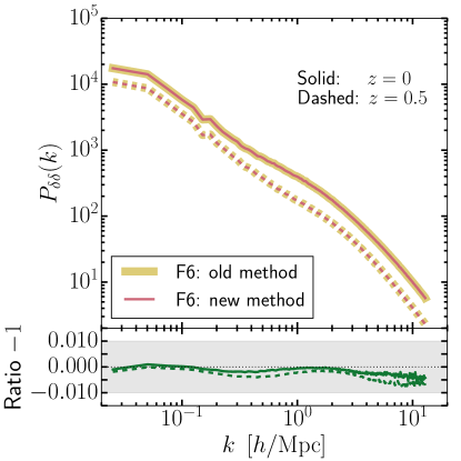
In Fig. 1, we compare the nonlinear matter power spectrum, , from the ‘Medium res’ simulations using the old and new methods. was computed using the publicly-available powmes code (powmes, ). The solid and dashed curves are computed at and , respectively, for F6. The results of the two methods are indistinguishable at both redshifts, and this is quantified more clearly in the bottom panel of Fig. 1, which shows the relative difference between the old and new methods. The shaded grey band in this panel represents a 1% error around zero; clearly, the new and old methods agree to well below 1% at all scales resolved in the simulation. The same is true even at higher redshift (, not shown). We have checked that the agreement also holds in the case of the velocity divergence power spectrum, , which, being just the first integral of the gravitational acceleration, would be more sensitive to differences in the gravitational forces between the two methods. Agreement for , which is calculated in a volume-weighted way, shows that the two methods agree well even in regions of the cosmic web that are not mass-dominated. This is not unexpected: after all, the new method solves the same equation of motion, without needing to use the approximate and inefficient Newton-Raphson scheme. As a consequence, the simulation is now significantly faster than before: the new method boosts the speed of the F6 calculation by a factor of 15 relative to the old implementation in ecosmog (see the last column of Table 1).
Two-point statistics such as the power spectrum offer a complete description of clustering properties only for Gaussian fields. Gravitational instability theory predicts that the nonlinear evolution induced by gravity drives away the PDF of these fields from Gaussianity at late times and small scales (see e.g., refs. jbc1993, ; bernardeau1994, ). This is reflected in growing skewness and kurtosis of cosmic density and velocity fields. theories show systematic deviations from CDM for these statistics, and these can therefore be used as a test of the theory (hlfc2013, ). We have computed PDFs and their higher-order moments for the density and velocity divergence fields to test how well the old and new methods agree beyond simple two-point statistics. We find that the differences are very small and comparable to the differences seen in the . As an additional test, we have also computed the Fourier mode decoherence functions (sydhf1992, ; cc2002, ), defined as Pearson correlation coefficients for the Fourier modes of the two fields:
where and are the density or velocity divergence fields for the runs computed using the two methods. when both fields being compared have Fourier modes at given that correspond exactly. The density and velocity divergence fields for the F6 runs using the two methods take for almost the entire range of , up until the Nyquist limit of the simulations. These tests reassure us that the density and velocity fields produced by the old and the new method are, for all practical purposes, indistinguishable.
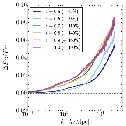
Results from the ‘High res’ simulations are shown in Fig. 2, where we plot the relative difference in of F6 with CDM – only results using the new method are shown. Curves of different colours represent the relative difference at different scale factors, as labelled in the legend. The legend labels also list the percentage overhead involved in the F6 simulation compared to the CDM run at the same scale factor. With the new method, the F6 simulation is now only slower than the CDM run at , and only slower at the final time. Compared to F6 simulations with comparable resolution using the old method (e.g., ref. liminality, ), the new implementation is estimated to be more than faster.
The degree to which the new method improves the efficiency of ecosmog over the old one depends on resolution. Indeed, in going from the ‘Low res’ to the ‘High res’ simulations, the gain in performance increases from a factor of 5 to a factor of over 20 (the overhead increases considerably with resolution in the old method). The improved efficiency of the numerical algorithm will enable us to run simulations of chameleon models that would previously have been computationally very expensive to perform. Future applications of the method could include running hydrodynamical simulations (where high resolution is required to follow accurately the hydrodynamics and to resolve spatial scales important for star formation and feedback), and running large numbers of low resolution volumes to estimate the covariance matrix in non-standard gravity.
V Summary and Discussions
Modified gravity models are an umbrella group of theories seeking to explain the apparent accelerated cosmic expansion by assuming modifications to the Einsteinian gravitational law on cosmological scales. Usually, such modifications must be small in high density environments in which gravity is known to be accurately described by GR, and this can be achieved by screening mechanisms, resulting in highly nonlinear field equations. Studying the cosmological implications of these theories and observational constraints on them is an active research topic in cosmology, but the nonlinear nature of these theories means that one has to resort to numerical simulations, which can be prohibitively slow. This has, up until now, limited the scope of accurately testing gravity using precision observational data.
In this paper, we proposed and demonstrated the power of a new and more efficient method to solve the nonlinear field equation in one of the most popular modified gravity models – the Hu-Sawicki variant of gravity. The current method used to simulate this model is slow mainly because of a variable redefinition aimed at making the relaxation algorithm numerically stable, but has the negative side effect of making the discrete equation even more nonlinear and, therefore, harder to converge. As a result, modified gravity simulations which match the size and resolution of the state-of-the-art CDM -body or hydrodynamical simulations have thus far been beyond reach (but see refs. hlmw2015, ; asp2016, ).
The new method avoids the specific variable redefinition used in the old method, and therefore does not further increase the nonlinearity of the discrete equation to be solved. More importantly, it enables the discrete equation to be written in a form that is analytically solvable at each Gauss-Seidel iteration. This is what ultimately makes the method efficient: compare solving a highly nonlinear algebraic equation analytically and solving the same equation using the Newton-Raphson iteration method (Eq. 14), and it is clear that the latter is generally much more inefficient.
We have performed test simulations using the new method, and confirmed that it is indeed very efficient. The working model for the tests is the F6 variant of Hu-Sawicki gravity. The chameleon screening is very efficient in F6, and it is therefore important that the nonlinear scalar field equations are solved accurately. In Fig. 1, we have confirmed that the new and old methods agree at the sub-percent level when comparing the nonlinear matter power spectrum, . The good agreement continues to hold at higher redshift, as well as for the velocity divergence power spectra, . Next, in Fig. 2, we presented results from our ‘High res’ simulations, which are comparable in resolution to the Millennium simulation. The total overhead in the F6 simulation is compared to the equivalent CDM run; this represents a boost in performance of compared to an F6 simulation of similar resolution using the old method.
The improved performance of the new simulation algorithm compared to the old one serves to highlight the importance of the way in which one discretises partial differential equations for the efficiency of numerically solving them. This is particularly true for highly nonlinear equations, such as those encountered in many modified gravity theories. Our work highlights the following:
(1) There is not a single way of discretisation, and this usually depends on the specific equations to be solved. In general, the discretisation should be chosen to preserve the original degree of nonlinearity of the equation as much as possible, and avoid further nonlinearising the equation.
(2) Where possible, exact solutions to the nonlinear discrete equation should be used instead of the approximate solution in Eq. (14). The latter, despite being commonly used in relaxation solutions to nonlinear differential equation, is a second option only for cases where has no analytical solution in general.
The same observations and conclusions apply to other classes of partial differential equations, such as those involving higher order powers of the derivatives of the scalar field (e.g., , , , ), which are commonly encountered in Vainshtein-type theories. In fact, in the most popular examples of such models – the DGP, cubic Galileon and quartic Galileon models – we also found that the discretisation could be done in a way such that is a quadratic or cubic equation that can be solved analytically. This fact has been used in lzk2013 ; letal2013 ; blhbp2013 ; bbl2015 to make simulations of these models possible, more efficient and free from numerical instabilities.
Unfortunately, the new method does not apply to all nonlinear partial differential equations, because it relies on being analytically solvable in the discrete equation. In the HS model with , satisfies a cubic equation, which does have analytical solutions. This neat property does not hold for other models. However, this method will still be very useful for the following reasons:
-
•
At the moment, no specific functional forms of – or more generally, no specific chameleon models – are known to be fundamental. Different models often share similar qualitative behaviours though the predictions can be quantitatively different. For what it is worth, the HS model serves as a great test case to gain insights into the question ‘How much deviation from GR (in the manner prescribed by the large class of chameleon models) is allowed by cosmological data?’. Indeed, all current observational constraints on modified gravity are to be considered as attempts to answer this question. In this context, the exact functional form of is not critical, because whatever form we adopt, it is unlikely to be the true theory. Actually, the HS model is capable of reproducing the behaviours of many classes of models, and is therefore a representative example.
-
•
There are other models that this method can be applied to. One example is the HS model with . In this case Eq. (17) becomes a quartic equation, which also has analytical solutions. A further example is the logarithmic model studied in the literature (e.g., ref. bbds2008, ):
where is the cosmological constant, and and are some model parameters. In this case, , and we could define so that Eq. (17) becomes a quadratic equation. Moreover, looking beyond gravity, there are also other chameleon models with different coupling strengths from the value of for models, and can be simulated using this method bdlwz2013 . The method can also be applied to the symmetron model hk2010 , in which the equation is a cubic equation dlmw2012 for the symmetron field , and certain variants of the dilaton model bbds2010 ; bdlwz2012 , though our initial tests showed that the improvement of the efficiency is far smaller than in the case (Appendix B).
Efforts towards generalising the new method to the models mentioned above, and to running large high resolution simulations including baryonic physics, are currently ongoing and will be the subject of future works.
Acknowledgements.
We thank the organisers of the 1st Mexican Numerical Simulations School held in Mexico City (03-06 October 2016), for inspiring discussions that motivated this study. We are also grateful to Fabian Schmidt for many enlightening comments. SB is supported by STFC through grant ST/K501979/1. BL acknowledges support by STFC Consolidated Grant Nos. ST/L00075X/1 and RF040365. WAH acknowledges support from the Polish National Science Center under contract #UMO-2012/07/D/ST9/02785. KK is supported by STFC grant ST/N000668/1. Both WAH & KK are also supported by the European Research Council through grant 646702 (CosTesGrav). CLL acknowledges ICRAR (University of Western Australia) and Queensland University for their warm hospitality and Chris Power and David Parkinson for discussions. CLL also acknowledges support from STFC consolidated grant ST/L00075X/1 as well as funding support from the University of Queensland - University of Western Australia Bilateral Research Collaboration Award. This work was supported by resources provided by The Pawsey Supercomputing Centre with funding from the Australian Government and the Government of Western Australia. The simulations described in this study used the DiRAC Data Centric system at Durham University, operated by the Institute for Computational Cosmology on behalf of STFC DiRAC HPC Facility (www.dirac.ac.uk). This equipment was funded by BIS National E-Infrastructure Capital grant ST/K00042X/1, STFC Capital grant ST/H008519/1, and STFC DiRAC Operations grant ST/K003267/1 and Durham University. DiRAC is part of the National E-Infrastructure. Part of this work was performed at the Aspen Center for Physics, which is supported by National Science Foundation grant PHY-1066293.Appendix A The poorer performance of the speed up truncation method in chameleon models
In bbl2015 , the authors proposed a method to speed up -body simulations of modified gravity models with Vainshtein screening. The speed up in this method is achieved by truncating the Gauss-Seidel iterations of the scalar field above a certain refinement level, and then computing the solution on those fine levels by interpolating from coarser levels. This approximate method agrees very well with the results of the full -body calculation (see bbl2015 for details) due to the fact that in Vainshtein screening models, there is a correlation between higher density regions (or, equivalently, higher refined regions in the simulation box) and screening efficiency. Even when the error induced on the fifth force on the refinements is large, it does not propagate to the total gravitational force because the amplitude of the fifth force is small/screened.
In chameleon models, however, the correlation between high density regions and screening efficiency becomes less marked because of the dependence on the environmental density (in Vainshtein models, the screening efficiency depends on the local density only). For example, in models, a low mass halo in a dark matter void constitutes an example of a highly-refined region (the centre of the halo can be very concentrated) that may not be screened (either by itself or by the low density environment it lives in). It is therefore interesting to determine whether or not the same truncation method, which works well for Vainshtein models, works equally well in chameleon-type theories.
Fig. 3 shows the relative difference of two truncated simulations to a full (ie., not truncated) simulation. The simulation box used for this test is the same as the ‘Medium res’ setup in the main text, but with (the so-called F5 model). The result is shown at three different redshifts and the two labelled truncation schemes are as follows. The case indicates that the scalar field was only explicitly solved on the coarse level, with this solution being interpolated to all finer levels. In the case of , the scalar field was explicitly solved on the coarse, first refinement and second refinement levels, with the solution at the second level being interpolated to all other finer levels. The values and indicate the cell size of the first truncated level in both these simulations, which ran, respectively, and times faster than the full run. For both these truncation criteria, the figure shows that the error can be kept for , but for higher modes, it grows to unacceptably large values. For example, at , the error is of .
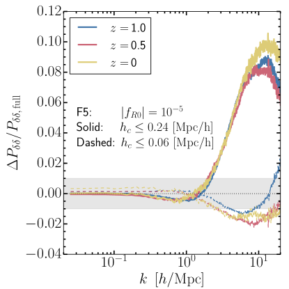
The result shown in Fig. 3 for should be contrasted with the corresponding picture in the DGP model (which employs Vainshtein screening), in which for the same truncation criteria, the error is always kept below for (see e.g., Fig. 5 of bbl2015 ). Furthermore, the method described in the main body of this paper results in comparable boosts in performance compared to previous simulations, but without any loss in accuracy. From this we can conclude that the truncation scheme that works well in Vainshtein screening models is not suitable for chameleon theories.
Appendix B Performance of the new method for the symmetron model
As a test of the performance of our new method for other classes of screening mechanisms, we implemented our method for the case of the symmetron model. The code used in this case, Isis (isis, ), is a modified version of ramses developed independently of ecosmog. Details of the symmetron model and its implementation in Isis are described in isis . Briefly, the equation of motion for the scalar field is given by:
| (25) |
where the quantity is a function of the parameters of the symmetron model. While the equation is formally equivalent to the in the main text (Eq. 6), the screening mechanism operates differently. In the model, the scalar field screens itself by becoming very massive. On the other hand, in the symmetron model, the screening occurs when a particular symmetry is restored (i.e., when the factor in front of the linear term of the source of Eq. (25) becomes positive). Consequently, the model behaves in a different manner to . For instance, negative solutions for the symmetron field, , are allowed and, thus, the constraints implemented in the case (§ III.2) are not required. We refer the reader to lp2014 for a summary of the complex phenomenology associated with this property of the symmetron field.
The nonlinear modified gravity solver in Isis is very similar to that of the model in ecosmog. The code uses an implicit multigrid solver with full approximation storage, which means that the code relies on a Newton-Raphson algorithm to evolve the solution in every step of the Gauss-Seidel iterations. As the discretised equation is cubic, the method proposed in this paper can be applied in a straightforward manner. As a check of the accuracy of the new method in solving the symmetron field equations, we have repeated satisfactorily the static test presented in the original Isis paper (Fig. 2 in ref. isis, ). However, we find that there is no major difference in the performance of the standard Isis implementation compared to using the new method, either in terms of the run time, or the convergence rate of the iterative solver.
In order to gauge the difference in computing time between the old and new methods for the symmetron model, we have run a set of five different realisations of a box of size on a side, containing particles. For each realisation, there are three sets of simulations: CDM and the symmetron model using the old and new methods. Overall, we do not find any improvement in the performance of Isis using the new method. For both the old and new methods, the overhead compared the CDM simulation is of the order of and, in fact, the run time using the new method is actually slower than using the default implementation - this is explained by the fact that more iterations were required for the whole set of five realisations using the new method. The convergence criterion on the residual was set to for both symmetron runs; we find that, unlike in the model, making the convergence criterion even stricter does not impact the run time of the symmetron simulations by a great amount.
The reason why the performance of the code appears to be insensitive to the details of the iteration scheme is seemingly related to the type of screening mechanism used by the symmetron model. The symmetron mechanism is based on a density threshold above which the solution very quickly approaches zero and thus decouples the scalar field from matter. This makes the solutions more stable and, therefore, not strongly dependent on the details of the solver employed. Since the default solver in Isis does not involve a nonlinear change of variables to force a stable, positive solution (as in the case), the performance is already similar to what ecosmog can do for using the new method.
References
- (1)
- (2) T. Clifton, P. G. Ferreira, A. Padilla and C. Skordis, Phys. Rept. 513 (2012) 1.
- (3) A. Joyce, L. Lombriser, & F. Schmidt, Ann. Rev. of Nuc. and Part. Sc., 66, 95, (2016).
- (4) E. J. Copeland, M. Sami and S. Tsujikawa, Int. J. Mod. Phys. D, 15, 1753 (2006).
- (5) J. Guy, M. Sullivan, A. Conley, N. Regnault, P. Astier, C. Balland et al., Astron. Astrophys. 523, A7 (2010).
- (6) W. J. Percival, B. A. Reid, D. J. Eisenstein, N. A. Bahcall, T. Budavari, J. A. Frieman et al., Mon. Not. R. Astron. Soc., 401, 2148 (2009).
- (7) F. Beutler, C. Blake, M. Colless, D. H. Jones, L. Staveley-Smith, L. Campbell et al., Mon. Not. R. Astron. Soc., 416, 3017 (2011).
- (8) B. A. Reid, L. Samushia, M. White, W. J. Percival, M. Manera, N. Padmanabhan et al., Mon. Not. R. Astron. Soc., 426, 2719 (2012).
- (9) G. Hinshaw, D. Larson, E. Komatsu, D. N. Spergel, C. L. Bennett, J. Dunkley et al. (2012), arXiv:1212.5226 [astro-ph.CO].
- (10) A. G. Riess, L. Macri, S. Casertano, M. Sosey, H. Lampeitl, H. C. Ferguson et al., Astrophys. J. 699, 539 (2009).
- (11) C .M. Will, The Confrontation between General Relativity and Experiment, Living Rev. Relativity, 17, 4 (2014).
- (12) J. Khoury and A. Weltman, Phys. Rev. D, 69, 044026 (2004).
- (13) D. F. Mota and D. J. Shaw, Phys. Rev. D, 75, 063501 (2007).
- (14) T. P. Sotiriou and V. Faraoni, Rev. Mod. Phys., 82, 451 (2010).
- (15) B. Li and J. D. Barrow, Phys. Rev. D 75, 084010 (2007).
- (16) W. Hu and I. Sawicki, Phys. Rev. D, 76, 064004 (2007).
- (17) P. Brax, C. van de Bruck, A. C. Davis and D. J. Shaw, Phys. Rev. D, 78, 104021 (2008).
- (18) J. Wang, L. Hui and J. Khoury, Phys. Rev. Lett., 109, 241301 (2012).
- (19) M. Raveri, B. Hu, N. Frusciante and A. Silverstri, Phys. Rev. D, 90, 043513 (2014).
- (20) J. Ceron-Hurtado, J. He and B. Li, Phys. Rev. D94, 064502 (2016).
- (21) P. Brax, C. van de Bruck, A. C. Davis and D. J. Shaw, Phys. Rev. D82, 063519 (2010).
- (22) K. Hinterbichler and J. Khoury, Phys. Rev. Lett., 104, 231301 (2010).
- (23) H. Oyaizu, Phys. Rev. D78, 123523 (2008).
- (24) H. Oyaizu, M. Lima and W. Hu, Phys. Rev. D, 78, 123524 (2008).
- (25) F. Schmidt, M. Lima, H. Oyaizu and W. Hu, Phys. Rev. D, 79, 083518 (2009).
- (26) B. Li and H. Zhao, Phys. Rev. D80, 044027 (2009).
- (27) H. Zhao, A. V. Maccio, B. Li, H. Hoekstra and M. Feix, Astrophys. J., 712L, 179 (2010).
- (28) C. Llinares, A. Knebe, & H. Zhao, Mon. Not. R. Astron. Soc., 391, 1778 (2008).
- (29) B. Li and H. Zhao, Phys. Rev. D81, 104047 (2010).
- (30) G. Zhao, B. Li and K. Koyama, Phys. Rev. D83, 044007 (2011).
- (31) G. Zhao, B. Li and K. Koyama, Phys. Rev. Lett., 107, 071303 (2011).
- (32) Y. Li and W. Hu, Phys. Rev. D84, 084033 (2011).
- (33) B. Li, G. Zhao and K. Koyama, Mon. Not. R. Astron. Soc., 421, 3481 (2012).
- (34) L. Lombriser, K. Koyama, G. Zhao and B. Li, Phys. Rev. D85, 124054 (2012).
- (35) J. Lee, G. Zhao, B. Li and K. Koyama (2012), Astrophys. J., 763, 28 (2013).
- (36) E. Jennings, C. M. Baugh, B. Li, G. Zhao and K. Koyama (2012), Mon. Not. R. Astron. Soc., 425, 2128 (2012).
- (37) B. Li, W. A. Hellwing, K. Koyama, G. Zhao, E. Jennings and C. M. Baugh, Mon. Not. R. Astron. Soc., 428, 743 (2013).
- (38) B. Li, G. Zhao, R. Teyssier and K. Koyama, J. Cosmo. Astropart. Phys., 01, 051 (2012).
- (39) R. Teyssier, Astron. Astrophys. 385 , 337-364 (2002).
- (40) P. Brax, A. C. Davis and B. Li (2011), Phys. Lett. B, 715, 38 (2012).
- (41) P. Brax, A. C. Davis, B. Li and H. A. Winther (2012), Phys. Rev. D86, 044015 (2012).
- (42) P. Brax, A. C. Davis, B. Li, H. A. Winther and G. Zhao (2012), J. Cosmo. Astropart. Phys., 10, 002 (2012).
- (43) P. Brax, A. C. Davis, B. Li, H. A. Winther and G. Zhao (2013), J. Cosmo. Astropart. Phys., 04, 029 (2013).
- (44) E. Puchwein, M. Baldi and V. Springel, Mon. Not. R. Astron. Soc., 436, 348 (2013).
- (45) C. Llinares, D. F. Mota and H. A. Winther, Astron. & Astrophys. 562, 78 (2014).
- (46) H. Wilcox, R. C. Nichol, G. B. Zhao, D. Bacon, K. Koyama and R. A. Kathy, Mon. Not. R. Astron. Soc., 462, 715 (2016).
- (47) H. A. Winther, F. Schmidt, A. Barreira, C. Arnold, S. Bose, C. Llinares, M. Baldi, B. Falck, W. A. Hellwing, K. Koyama, B. Li, D. F. Mota, E. Puchwein, R. E. Smith and G. B. Zhao, Mon. Not. R. Astron. Soc., 454, 4208 (2015).
- (48) G. Dvali, G. Gabadadze and M. Porrati, Phys. Lett. B485, 208 (2000).
- (49) P. Brax and P. Valageas, Phys. Rev. D90, 023507 (2014).
- (50) P. Brax and P. Valageas, Phys. Rev. D90, 023508 (2014).
- (51) A. I . Vainshtein, Phys. Lett. B39, 393 (1972).
- (52) C. de Rham, G. Gabadadze and A. J. Tolley, Phys. Rev. Lett. 106 231101 (2011).
- (53) F. Sbisa, G. Niz, K. Koyama and G. Tasinato, Phys. Rev. D86 024033 (2012).
- (54) G. Chkareuli and D. Pirtskhalava, Phys. Lett. B713, 99 (2012).
- (55) A. Nicolis, R. Rattazzi and E. Trincherini, Phys. Rev. D79, 064036 (2009).
- (56) C. Deffayet, C. Esposito-Farese and A. Vikman, Phys. Rev. D79, 084003 (2009).
- (57) C. Burrage and D. Seery, J. Cosmo. Astropart. Phys., 08 011 (2010).
- (58) N. Kaloper, A. Padilla and N. Tanahashi, JHEP 10 148 (2011).
- (59) A. De Felice, R. Kase and S. Tsujikawa, Phys. Rev. D85 044059 (2012).
- (60) R. Kimura, T. Kobayashi and K. Yamamoto, Phys. Rev. D85 024023 (2012).
- (61) N. Chow and J. Khoury, Phys. Rev. D80, 024037 (2009).
- (62) F. P. Silva and K. Koyama, Phys. Rev. D80, 121301 (2009).
- (63) R. Gannouji and M. Sami, Phys. Rev. D82, 024011 (2010).
- (64) A. De Felice and S. Tsujikawa, Phys. Rev. Lett., 105, 111301 (2010).
- (65) S. Nesseris, A. De Felice and S. Tsujikawa, Phys. Rev. D82, 124054 (2010).
- (66) A. Ali, R. Gannouji and M. Sami, Phys. Rev. D82, 103015 (2010).
- (67) P. Brax, C. Burrage and A. C. Davis, J. Cosmo. Astropart. Phys., 09, 020 (2011).
- (68) S. A. Appleby and E. V. Linder, J. Cosmo. Astropart. Phys., 03, 043 (2012).
- (69) S. A. Appleby and E. V. Linder, J. Cosmo. Astropart. Phys., 08, 026 (2012).
- (70) A. Barreira, B. Li, C. M. Baugh and S. Pascoli, Phys. Rev. D86, 124016 (2012).
- (71) J. Neveu, V. Ruhlmann-Kleider, A. Conley, N. Palanque-Delabrouille, P. Astier, J. Guy and E. Babichev, Astron. & Astrophys., 555, 53 (2013).
- (72) A. Barreira, B. Li, A. Sanchez, C. M. Baugh and S. Pascoli, Phys. Rev. D83, 103511 (2013).
- (73) A. Barreira, B. Li, W. A. Hellwing, L. Lombriser, C. M. Baugh and S. Pascoli, J. Cosmo. Astropart. Phys., 04, 029 (2014).
- (74) B. Falck, K. Koyama, G. B. Zhao and B. Li, J. Cosmo. Astropart. Phys., 07, 058 (2014).
- (75) B. Falck, K. Koyama and G. B. Zhao, J. Cosmo. Astropart. Phys., 07, 049 (2015).
- (76) H. Okada, T. Totani and S. Tsujikawa, Phys. Rev. D87, 103002 (2013).
- (77) M. Wyman, E. Jennings and M. Lima, Phys. Rev. D88, 084029 (2013).
- (78) Y. Zu, D. H. Weinberg, E. Jennings, B. Li and M Wyman, Mon. Not. R. Astron. Soc., 445, 1885 (2014).
- (79) A. Barreira, S. Bose, B. Li and C. Llinares, 2016, arXiv:1605.08436 [astro-ph.CO].
- (80) J. Neveu, V. Ruhlmann-Kleider, P. Astier, M. Besancon J. Guy, A. Moller and E. Babichev (2016), arXiv: 1605.02627 [astro-ph.CO].
- (81) A. Merloni, et al. (2012), arXiv:1209.3114 [astro-ph.CO] (http://www.mpe.mpg.de/eROSITA/).
- (82) R. Laureijs, et al., Euclid Definition Study Report (2011), arXiv:1110.3193 [astro-ph.CO] (http://desi.lbl.gov/).
- (83) DESI Collaboration, A. Aghamousa, J. Aguilar, et al. (2016), arXiv:1611.00036 [astro-ph.CO].
- (84) DESI Collaboration, A. Aghamousa, J. Aguilar, et al. (2016), arXiv:1611.00037 [astro-ph.CO].
- (85) M. Levi, et al. (2013), arXiv:1308.0847 [astro-ph.CO] (http://www.euclid-ec.org/).
- (86) Z. Ivezic, et al. (2008), arXiv:0805.2366 (http://www.lsst.org/).
- (87) K. Koyama, Reports on Progress in Physics, 79, 046902 (2016).
- (88) H. A. Winther and P. G. Ferreira, Phys. Rev. D91, 123507 (2015).
- (89) A. Barreira, S. Bose and B. Li, J. Cosmo. Astropart. Phys., 12, 059 (2015).
- (90) B. Li and G. Efstathiou, Mon. Not. R. Astron. Soc., 421, 1431 (2012).
- (91) G. B. Zhao, Astrophys. J. Suppl., 211, 23 (2014).
- (92) A. Mead, J. Peacock, L. Lombriser and B. Li, Mon. Not. R. Astron. Soc., 452, 4203 (2015).
- (93) M. Cataneo, D. Rapetti, L. Lombriser and B. Li (2016), arXiv:1607.08788 [astro-ph.CO].
- (94) S. Bose, W. A. Hellwing, & B. Li, J. Cosmo. Astropart. Phys., 2, 034, (2015).
- (95) B. Jain, V. Vikram and J. Sakstein, Astrophys. J., 779, 39 (2013).
- (96) V. Vikram, A. Cabre, B. Jain and J. T. Van der Plas, J. Cosmo. Astropart. Phys., 08, 020 (2013).
- (97) L. Lombriser, Annalen der Physik, 526, 259 (2014).
- (98) C. Burrage, & J. Sakstein (2016), arXiv:1609.01192 [astro-ph.CO].
- (99) A. Terukina, L. Lombriser, K. Yamamoto et al., J. Cosmo. Astropart. Phys., 4, 013 (2014).
- (100) H. Wilcox, D. Bacon, R. .C. Nichol et al., Mon. Not. R. Astron. Soc., 452, 1171 (2015).
- (101) M. Cataneo, D. Rapetti, F. Schmidt, A. B. Mantz, S. W. Allen, D. E. Applegate, P. L. Kelly, A. von der Linden and R. Glenn Morris, Phys. Rev. D92, 044009 (2015).
- (102) X. Liu, B. Li, G. B. Zhao, M. C. Chiu, W. Fang, C. Pan, Q. Wang, W. Du, S. Yuan, L. Fu and Z. Fan, Phys. Rev. Lett., 117, 051101 (2016).
- (103) Y. Cai, N. Padilla and B. Li, Mon. Not. R. Astron. Soc., 451, 1036 (2015).
- (104) S. Peirone, M. Raveri, M. Viel, S. Borgani and S. Ansoldi (2016), arXiv:1607.07863 [astro-ph.CO].
- (105) H. Martel and P. R. Shapiro, Mon. Not. R. Astron. Soc., 297, 467 (1998).
- (106) A. Brandt, Math. of Comp., 31, 333 (1977).
- (107) V. Springel, S. D. M. White, A. Jenkins et al.. Nature (London), 435, 629 (2005).
- (108) Planck Collaboration, P. A. R. Ade, N. Aghanim et al., Astron. & Astrophys., 594, A13 (2016).
- (109) E. Komatsu, K. M. Smith, J. Dunkley et al., Astrophys. J. Suppl., 192, 18 (2011).
- (110) S. Colombi, A. H. Jaffe, D. Novikov and C. Pichon, Mon. Not. R. Astron. Soc., 393, 511 (2009).
- (111) R. Juszkiewicz, F. R. Bouchet, & S. Colombi, Astrophys. J., 412, L9 (1993).
- (112) F. Bernardeau, Astrophys. J., 433, 1 (1994).
- (113) W. A. Hellwing, B. Li, C. S. Frenk, S. Cole, Mon. Not. R. Astron. Soc., 435, 2806 (2013).
- (114) M. A. Strauss, A. Yahil, M. Davis, J. P. Huchra, & K. Fisher, Astrophys. J., 397, 395 (1992).
- (115) M. J. Chodorowski, & P. Ciecielag, Mon. Not. R. Astron. Soc., 331, 133 (2002).
- (116) D. Shi, B. Li, J. Han, L. Gao, & W. A. Hellwing, Mon. Not. R. Astron. Soc., 452, 3179 (2015).
- (117) A. Hammami, C. Llinares, D. F. Mota, & H. A. Winther, Mon. Not. R. Astron. Soc., 449, 3635 (2015).
- (118) C. Arnold, V. Springel, & E. Puchwein, Mon. Not. R. Astron. Soc., 462, 1530 (2016).
- (119) B. Li, G. B. Zhao and K. Koyama, J. Cosmo. Astropart. Phys., 05, 023 (2013).
- (120) B. Li, A. Barreira, C. M. Baugh, W. A. Hellwing, K. Koyama, S. Pascoli and G. B. Zhao, J. Cosmo. Astropart. Phys., 11, 012 (2013).
- (121) A. Barreira, B. Li, W. A. Hellwing, C. M. Baugh and S. Pascoli, J. Cosmo. Astropart. Phys., 10, 027 (2013).
- (122) A. C. Davis, B. Li, D. F. Mota and H. A. Winther, Astrophys. J. 748, 61 (2012)
- (123) C. Llinares & L. Pogosian, Phys. Rev. D 90, 124041 (2014).