Holographic Kondo and Fano Resonances

Abstract

We use holography to study a $(1+1)$-dimensional Conformal Field Theory (CFT) coupled to an impurity. The CFT is an $SU(N)$ gauge theory at large $N$, with strong gauge interactions. The impurity is an $SU(N)$ spin. We trigger an impurity Renormalization Group (RG) flow via a Kondo coupling. The Kondo effect occurs only below the critical temperature of a large-$N$ mean-field transition. We show that at all temperatures $T$, impurity spectral functions exhibit a Fano resonance, which in the low-$T$ phase is a large-$N$ manifestation of the Kondo resonance. We thus provide an example in which the Kondo resonance survives strong correlations, and uncover a novel mechanism for generating Fano resonances, via RG flows between $(0+1)$-dimensional fixed points.

I Introduction

The Kondo effect is the screening of an impurity spin by a Landau Fermi Liquid (LFL) at low $T$ Kondo (1964); Hewson (1993). A variety of techniques, such as Wilson’s RG, large-$N$, CFT, and more Cox and Zawadowski (1998), have captured many characteristic Kondo phenomena. Nevertheless, many questions resist solution, for example about inter-impurity interactions, subsystem Entanglement Entropy (EE), non-equilibrium processes like quantum quenches, and more.

In particular, what happens when the LFL is replaced with strongly correlated electrons? For example, how does the Kondo effect change in a Luttinger liquid Lee and Toner (1992); Furusaki and Nagaosa (1994); Fröjdh and Johannesson (1995, 1996); Furusaki (2005) or the Hubbard model Fulde et al. (1993); Schork and Fulde (1994)? In the latter case, experiments reveal dramatic effects of strong correlations, such as enhancement of the Kondo temperature, $T_{K}$. On the theory side, although special tools like bosonization Lee and Toner (1992); Furusaki and Nagaosa (1994); Fröjdh and Johannesson (1995, 1996); Furusaki (2005) and uncontrolled mean-field approximations Fulde et al. (1993); Khaliullin and Fulde (1995); Igarashi et al. (1995); Tornow et al. (1997); Schork and Blawid (1997); Davidovich and Zevin (1998); Duc and Thang (1999); Hofstetter et al. (2000) have provided insight, in general, reliable techniques do not yet exist to answer questions about Kondo phenomena in strongly-correlated systems.

To address all of the above, we have developed an alternative Kondo model, based on holographic duality Erdmenger et al. (2013); O’Bannon et al. (2016); Erdmenger et al. (2016, 2015). Our model replaces the LFL by a $(1+1)$-dimensional CFT in which spin $SU(2)$ is replaced by gauged $SU(N)$, with large $N$ and strong gauge interactions. Our model has already revealed novel strong-coupling phenomena in RG Erdmenger et al. (2013); O’Bannon et al. (2016), inter-impurity interactions O’Bannon et al. (2016) and EE Erdmenger et al. (2016).

Here we initiate the study of non-equilibrium phenomena in our model: we compute linear response (Green’s) functions of a charged bosonic impurity operator, $\mathcal{O}$, in our model. We have two main results.

First, we find a large-$N$ manifestation of the Kondo resonance Hewson (1993); Phillips (2012); Coleman (2015), a signature of the Kondo effect. As expected, our Kondo resonance appears only at $T$ below the critical temperature $T_{c}$ of a mean-field transition that is common to large-$N$ Kondo models Coleman and Andrei (1986); Coleman (1987); Senthil et al. (2003, 2004); Coleman (2015): $\langle\mathcal{O}\rangle$ becomes non-zero when $T\leq T_{c}$. We thus prove unequivocally that our holographic model realizes a genuine Kondo effect, as opposed to some other impurity physics, and furthermore show that a large-$N$ Kondo resonance can survive strong correlations essentially intact.

Second, at all $T$, $\mathcal{O}$’s spectral function exhibits a Fano resonance Fano (1961); Miroshnichenko et al. (2010), which occurs when a Lorentzian resonance is immersed in a continuum of states (in energy). A Fano resonance is characterized not only by its position, width, and height, like a Lorentzian, but also by an asymmetry parameter, $q$, which measures the relative strength of resonant versus non-resonant scattering. Our $q$ increases as $T\to T_{c}^{+}$. When $T\leq T_{c}$, the Fano line-shape arises from our Kondo resonance, which must be anti-symmetric due to Particle-Hole Symmetry (PHS), and hence has the special value $q=1$.

Although Fano resonances have been observed in many impurity systems in one spatial dimension Madhavan et al. (1998, 2001); Göres et al. (2000); Miroshnichenko et al. (2010), ours arise from a qualitatively different mechanism. For instance, in side-coupled quantum dots (QDs) Madhavan et al. (2001); Göres et al. (2000); Miroshnichenko et al. (2010) the Lorentzian resonances are the discrete states on the QD, and the continuum comes from electronic scattering states in the leads. Coupling the two, for example by a Kondo coupling, can then produce Fano resonances.

Our model also has an impurity coupled to a continuum in one spatial dimension, i.e. the CFT. However, our model has two couplings: the CFT’s $SU(N)$ gauge coupling and the Kondo coupling. The spectral function of $\mathcal{O}$ inherits $(0+1)$-dimensional scale invariance from the former, and so exhibits a continuum of states, in contrast to a QD’s discrete states. The Kondo coupling then triggers an RG flow from that $(0+1)$-dimensional fixed point, and creates a resonance that cannot escape the continuum, hence producing a Fano line-shape.

To our knowledge, such a mechanism for producing Fano resonances is novel, and moreover is easy to generalize to any RG flow between $(0+1)$-dimensional fixed points, as follows. Scale invariance implies that any spectral function will be a featureless continuum, which in $(0+1)$ dimensions means a power law (or logarithm) in frequency. A relevant deformation can then explicitly break scale invariance, trigger an RG flow to an IR fixed point—in which case we expect the continuum to survive—and may also produce resonances. In higher dimensions, the resonances would not have to be within the continuum, for example the two could be separated in momentum space. However, in $(0+1)$ dimensions the resonances have no place to escape the continuum, and hence must produce Fano line-shapes.

In fact, such a mechanism was at work in some previous cases, such as the large-$N$ Kondo model at sufficiently low $T$ Parcollet et al. (1998), and holographic duals of $T=0$ charged black branes Faulkner et al. (2011a, b); Sachdev (2015). However, the resulting Fano resonances went unidentified, leaving crucial physics overlooked, namely the relative strength of resonant versus non-resonant scattering, as measured by $q$. Our results not only provide a novel perspective on these cases, but also predict Fano resonances in RG flows between other $(0+1)$-dimensional fixed points, such as Sachdev-Ye-Kitaev fixed points Sachdev and Ye (1993); Kitaev (2015); Sachdev (2015); Polchinski and Rosenhaus (2016); Jevicki et al. (2016); Maldacena and Stanford (2016); Jevicki and Suzuki (2016); Witten (2016).

Further results of our model, including details of holographic renormalization useful for holographic impurity models in general, will appear in Erdmenger et al. (2017).

II Holographic Kondo Model

We first briefly review some essential features of the CFT and large-$N$ approaches to the Kondo model, and how our model builds upon and extends them.

The CFT approach Affleck (1995) is based on s-wave reduction of LFL fermions about the impurity, plus linearization of the dispersion relation. In/out-going s-waves become relativistic left/right-moving fermions, $\psi_{L}$ and $\psi_{R}$, in the radial direction, $r$. Reflecting $\psi_{R}$ to $r<0$ and relabeling $\psi_{R}\to\psi_{L}$ leads to $\psi_{L}$ alone on the entire $r$ axis, with impurity at $r=0$. The $\psi_{L}$ form a $(1+1)$-dimensional chiral CFT with $SU(2)_{1}\times U(1)$ spin and charge Kac-Moody currents, respectively. In the Hamiltonian, the Kondo interaction is $\delta(r)g_{K}S^{A}J^{A}$, with coupling constant $g_{K}$, impurity spin $S^{A}$, and spin current $J^{A}$, $A=1,2,3$. An antiferromagnetic coupling, $g_{K}>0$, is marginally relevant, and triggers an RG flow to an IR chiral CFT characterized by a phase shift of $\psi_{L}$ and impurity screening Affleck (1995).

The large-$N$ approach begins by replacing spin $SU(2)\to SU(N)$, followed by $N\to\infty$ with $\lambda_{K}\equiv Ng_{K}$ fixed Bickers, N. (1987); Cox and Zawadowski (1998); Coleman (2007, 2015). We will only consider $S^{A}$ in totally anti-symmetric $SU(N)$ representations of rank $\mathcal{Q}$, and introduce Abrikosov pseudo-fermions $\chi$ via $S^{A}=\chi^{\dagger}T^{A}\chi$, with $SU(N)$ generators $T^{A}$, $A=1,\ldots,N^{2}-1$. Doing so introduces an auxiliary $U(1)$ acting only on $\chi$, but with charge fixed by projecting onto states with $\chi^{\dagger}\chi=\mathcal{Q}$. At large $N$, $S^{A}J^{A}=-\mathcal{O}^{\dagger}\mathcal{O}/2$ with $\mathcal{O}\equiv\psi_{L}^{\dagger}\chi$ O’Bannon et al. (2016), which is charged under both the charge and auxiliary $U(1)$’s.

Our holographic model Erdmenger et al. (2013) begins by gauging $SU(N)$, thus introducing the ’t Hooft coupling, $\lambda$. We then add degrees of freedom to make the gauge theory a $(1+1)$-dimensional CFT with sparse operator spectrum when $N$ and $\lambda$ both $\to\infty$, but whose details otherwise are irrelevant. The theory is then holographically dual to Einstein-Hilbert gravity in $(2+1)$-dimensional Anti-de Sitter space, $AdS_{3}$ Aharony et al. (2000). The charge $U(1)$ Kac-Moody current is dual to a $U(1)$ Chern-Simons gauge field, $A$, the auxiliary $U(1)$ is dual to a Maxwell field $a$ on an $AdS_{2}$ defect at $r=0$, and $\mathcal{O}$ is dual to a complex scalar field $\Phi$ also in $AdS_{2}$, charged under both $A$ and $a$. As long as the stress-energy tensor is finite, at large $N$ we can neglect back-reaction of $A$, $a$, $\Phi$ (dual to fundamental fields) on the geometry (dual to adjoint fields). When $T>0$, the bulk metric is thus the BTZ black brane,

$$ds^{2}=\frac{1}{z^{2}}\left(h^{-1}(z)\mathrm{d}z^{2}-h(z)\mathrm{d}t^{2}+\mathrm{d}r^{2}\right),$$

with $h(z)=1-z^{2}/z_{H}^{2}$ where $z_{H}=1/2\pi T$, and unit AdS radius. The fields $a$ and $\Phi$ are localised to the asymptotically $AdS_{2}$ subspace at $r=0$, with induced metric $g_{mn}$ ($m,n=z,t$). We describe the dynamics of $A$, $a$, and $\Phi$ by the simple quadratic action Erdmenger et al. (2013),

$$S =-\frac{N}{4\pi}\int\limits_{\textrm{BTZ}}A\wedge\mathrm{d}A+S_{AdS_{2}}\;,$$ (1a)

$$S_{AdS_{2}} =-N\int\limits_{x=0}\mathrm{d}z\mathrm{d}t\sqrt{-g}\Big{(}\frac{1}{4}f^{mn}f_{mn}$$ (1b)

$$\quad\quad\quad\quad\quad+\left(D^{m}\Phi\right)^{\dagger}\left(D_{m}\Phi\right)+M^{2}\Phi^{\dagger}\Phi\Big{)},$$

with field strength $f=\mathrm{d}a$, covariant derivative $D_{m}\Phi=\left(\partial_{m}+iA_{m}-ia_{m}\right)\Phi$, and mass-squared $M^{2}$. At the horizon $z=z_{H}$ we require regularity of all fields. At the boundary $z=0$, $a$’s leading mode, $a\sim Q/z$, is related to ${\cal Q}$: $Q\neq 0$ breaks $\chi$’s PHS, so the PHS value $Q=0$ is dual to the PHS value $\mathcal{Q}=N/2$, and increasing $|Q|$ corresponds to increasing $|\mathcal{Q}-N/2|$.

The large-$N$ Kondo interaction $-\lambda_{K}\mathcal{O}^{\dagger}\mathcal{O}/2$ is classically marginal, hence $\mathcal{O}$ has UV dimension $\Delta=1/2$, which fixes $M^{2}$ and hence $\Phi$’s near-boundary expansion, $\Phi\sim\sqrt{z}\left(\alpha\log z+\beta\right)$. Introducing the Kondo interaction amounts to adding a boundary term $\propto-\lambda_{K}\mathcal{O}^{\dagger}\mathcal{O}/2$ to $S$, which changes $\Phi$’s boundary condition from $\alpha=0$ to $\alpha=-\lambda_{K}\beta$ Witten (2001); Papadimitriou (2007); Erdmenger et al. (2013). For more details about the boundary terms, see O’Bannon et al. (2016); Erdmenger et al. (2017). A holographic scaling analysis reveals that $\lambda_{K}$ runs logarithmically, $\lambda_{K}=1/\log\left(T/T_{K}\right)$, diverging at the dynamically-generated Kondo temperature, $T_{K}\equiv\Lambda\,e^{-1/\lambda_{K}}/(2\pi)$, with $\lambda_{K}$ evaluated at the UV cutoff, $\Lambda$. A holographic antiferromagnetic UV Kondo coupling, $\lambda_{K}>0$, is thus marginally relevant, breaks conformal invariance, and triggers an RG flow.

As mentioned above, our model has a mean-field phase transition Erdmenger et al. (2013): $\langle\mathcal{O}\rangle=0$ ($\Phi=0$) when $T>T_{c}$ and $\langle\mathcal{O}\rangle\neq 0$ ($\Phi\neq 0$) when $T\leq T_{c}$. Condensate formation $\langle\mathcal{O}\rangle\neq 0$ breaks the charge and auxiliary $U(1)$’s to the diagonal, and signals the Kondo effect, including a phase shift of $\psi_{L}$, dual to a Wilson line of $A$, and impurity screening, dual to reduction of $f$ flux between $z=0$ and $z=z_{H}$. We refer to the $T>T_{c}$ and $T\leq T_{c}$ phases as “unscreened” and “screened,” respectively. In Erdmenger et al. (2013); O’Bannon et al. (2016); Erdmenger et al. (2016, 2015) we computed $T_{c}$ numerically. Below we obtain an exact formula for $T_{c}$.

III Fano Resonances

If a retarded Green’s function of complex frequency $\omega$, $G(\omega)$, has a pole at $\omega_{p}$, $G(\omega)\sim\frac{Z}{\omega-\omega_{p}}$, with complex residue $Z=Z_{R}+iZ_{I}$, then near the pole the spectral function $\rho(\omega)\equiv-2\,\textrm{Im}(G(\omega))$ will have a Fano resonance Fano (1961); Miroshnichenko et al. (2010) (setting $\textrm{Im}(\omega)=0$),

$$\rho_{Fano}(\omega)=\frac{(\omega-\omega_{0}+q\,\Gamma/2)^{2}}{(\omega-\omega_{0})^{2}+(\Gamma/2)^{2}}\,,$$ (2)

with position $\omega_{0}=\textrm{Re}(\omega_{p})$, width $\Gamma=2|\textrm{Im}(\omega_{p})|$, and asymmetry parameter $q=-Z_{R}/Z_{I}+\sqrt{1+Z_{R}^{2}/Z_{I}^{2}}$. Fano resonances are anti-symmetric when $q=1$, meaning $\rho(\omega)$ is odd under PHS, and symmetric when $q=0$ (an anti-resonance) or $\infty$ (a Lorentzian), meaning $\rho(\omega)$ is even. Fano resonances arise when a Lorentzian resonance is immersed in a continuum (in energy), due to interference between the two. The asymmetry parameter $q$ contains key dynamical information, specifically, $q^{2}\propto$ the ratio of probabilities of resonant and non-resonant scattering.

In our model, the $AdS_{2}$ subspace inherits scale invariance from $AdS_{3}$, or in dual field theory language, the impurity inherits scale invariance from the CFT, so $\rho(\omega)$ of impurity operators must be a featureless continuum. Our marginally-relevant Kondo coupling then breaks scale invariance and produces a resonance, while $Q\neq 0$ breaks PHS. We will show that $\rho(\omega)$ of $\mathcal{O}$ then indeed generically exhibits asymmetric Fano resonances.

IV Spectral Functions

We compute $G(\omega)$ holographically by solving for linearized fluctuations about solutions for the unscreened and screened phases Son and Starinets (2002); Kovtun and Starinets (2005); Erdmenger et al. (2017). At all $T$, we find that the Kac-Moody current’s $G(\omega)$ is unaffected by the impurity. In the unscreened phase, we find that all charged $G(\omega)$ vanish, i.e. $G_{\mathcal{O}\mathcal{O}}(\omega)\equiv\langle\mathcal{O}(\omega)\mathcal{O}(-\omega)\rangle=0$, while

$$G_{\mathcal{O}^{\dagger}\mathcal{O}}(\omega)\equiv\langle\mathcal{O}^{\dagger}(\omega)\mathcal{O}(-\omega)\rangle=\frac{N}{\lambda_{K}}\left(1-\frac{1}{\lambda_{K}D(\omega)}\right),$$

$$D(\omega)\equiv H\left[-\frac{1}{2}+iQ-\frac{i\omega}{2\pi T}\right]+H\left[-\frac{1}{2}-iQ\right]+\ln\left(\frac{2T}{T_{K}}\right),$$

with Harmonic number $H[x]$, and $\lambda_{K}$ evaluated at $\Lambda$. The form of $G_{\mathcal{O}\mathcal{O}^{\dagger}}(\omega)$ is the same, but with $Q\to-Q$. Scale invariance in $(0+1)$-dimensions and $\Delta=1/2$ imply a trivial UV continuum: $\lim_{\omega\to\infty}\rho_{\mathcal{O}^{\dagger}\mathcal{O}}(\omega)=0$.

For given $Q$ and $T$, $G_{\mathcal{O}^{\dagger}\mathcal{O}}(\omega)$ has poles in $\omega$ when $D(\omega)=0$. Fig. 1 shows our numerical results for the positions of the lowest (closest to $\omega=0$) and next-lowest poles of $G_{\mathcal{O}^{\dagger}\mathcal{O}}(\omega)$ and $G_{\mathcal{O}\mathcal{O}^{\dagger}}(\omega)$ in the complex $\omega/(2\pi T)$ plane, for $Q=1/2$. Other $Q$ give similar results. As $T\to T_{c}^{+}$, the lowest pole moves towards the origin, arrives there at $T_{c}$, and when $T<T_{c}$, crosses into the $\textrm{Im}(\omega)>0$ region, signaling instability (not shown). We thus identify $T_{c}$ as the $T$ where $D(\omega=0)=0$,

$$T_{c}=\frac{1}{2}\,T_{K}\,\textrm{exp}\left[-2\,\mathrm{Re}\left(H\left[\frac{1}{2}+iQ\right]\right)\right].$$

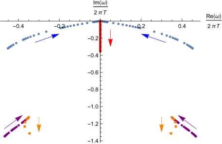
Figure 1: Positions of poles in the complex $\omega/(2\pi T)$ plane for $Q=1/2$. Blue and purple denote lowest and next-lowest poles, respectively, of $G_{\mathcal{O}^{\dagger}\mathcal{O}}(\omega)$ ($\textrm{Re}(\omega)>0$) and $G_{\mathcal{O}\mathcal{O}^{\dagger}}(\omega)$ ($\textrm{Re}(\omega)<0$), for $T/T_{c}$ from $100$ down to $1.001$. Red and orange denote the same for $G_{\mathcal{O}^{\dagger}\mathcal{O}}(\omega)$ for $T/T_{c}$ from $1$ down to $0.2$ Arrows indicate movement of poles as $T$ decreases.

Fig. 2 shows the normalized spectral function $\bar{\rho}_{\mathcal{O}^{\dagger}\mathcal{O}}(\omega)\equiv-2\frac{\lambda_{K}^{2}}{N}\,\mathrm{Im}\,G_{\mathcal{O}^{\dagger}\mathcal{O}}(\omega)$ versus real $\omega/(2\pi T)$ for $Q=1/2$ and $T/T_{c}=16,8,4,2$. We find a Fano resonance, as advertised, with asymmetric minimum and maximum. Numerically, $\omega_{0}\approx\textrm{Re}(\omega_{p})$ and $\Gamma\approx 2|\textrm{Im}(\omega_{p})|$, as in (2), where $\omega_{p}$ is $G_{\mathcal{O}^{\dagger}\mathcal{O}}(\omega)$’s lowest pole. As $T\to T_{c}^{+}$, $q$ grows: $q\approx 1.7$ at $T=16T_{c}$ while $q\approx 4$ at $T=2T_{c}$.

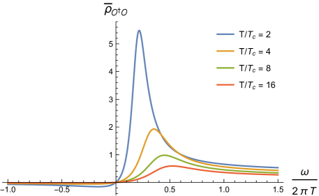
Figure 2: The normalized spectral function $\bar{\rho}_{\mathcal{O}^{\dagger}\mathcal{O}}(\omega)$ versus real $\omega/(2\pi T)$ for $Q=1/2$ and, from shortest to tallest, $T/T_{c}=16$ (red), $8$ (green), $4$ (orange), and $2$ (blue).

For $T$ just above $T_{c}$, $T\gtrsim T_{c}$, expanding in $T$ about $T_{c}$ and in $\omega$ about $\omega=0$ gives, for $G_{\mathcal{O}^{\dagger}\mathcal{O}}(\omega)$’s lowest pole,

$$\frac{\omega_{p}}{2\pi T}=-i\frac{T/T_{c}-1}{\psi^{\prime}[\frac{1}{2}+iQ]}\,,\quad Z=-i\frac{N}{\lambda_{K}^{2}}\frac{2\pi T_{c}}{\psi^{\prime}[\frac{1}{2}+iQ]},$$ (3)

with digamma function $\psi[x]$. The resonance height thus grows as $(T/T_{c}-1)^{-1}$ and the width shrinks as $T/T_{c}-1$. It is therefore not related to a Kondo resonance, which grows logarithmically as $T\to T_{K}^{+}$ Phillips (2012). Indeed, at large $N$ we expect the Kondo resonance only in the screened phase Coleman (2015). Our resonance is presumably a bound state of $\psi_{L}$ and $\chi$, heralding the nascent screened phase.

The $Z$ in (3) gives $q$ that depends only on $Q$, shown in fig. 3. (Anti-)symmetric values $q=1,0,\infty$ occur when $Q\to 0,\mp\infty$, respectively. Indeed, fig. 4 shows that even for relatively modest $Q=1$, the resonance is nearly Lorentzian, the minimum having practically vanished.

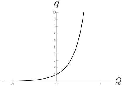
Figure 3: Asymmetry parameter $q$ versus $Q$, for $T\gtrsim T_{c}$.

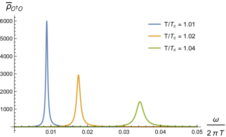
Figure 4: The normalized spectral function, $\bar{\rho}_{\mathcal{O}^{\dagger}\mathcal{O}}(\omega)$, versus real $\omega/(2\pi T)$ for $Q=1$ and, from shortest to tallest, $T/T_{c}=1.04$ (green), $1.02$ (orange), and $1.01$ (blue).

In the screened phase, we have numerical results for $G_{\mathcal{O}^{\dagger}\mathcal{O}}(\omega)$ Erdmenger et al. (2013); O’Bannon et al. (2016); Erdmenger et al. (2016, 2015, 2017). Fig. 1 shows our numerical results for the positions of the lowest and next-lowest poles in $G_{\mathcal{O}^{\dagger}\mathcal{O}}(\omega)$ for $Q=1/2$. Other $Q$ give similar results. At $T=T_{c}$ the poles are coincident with those of $G_{\mathcal{O}^{\dagger}\mathcal{O}}(\omega)$ and $G_{\mathcal{O}\mathcal{O}^{\dagger}}(\omega)$ in the unscreened phase. As $T$ decreases below $T_{c}$, $G_{\mathcal{O}^{\dagger}\mathcal{O}}(\omega)$’s lowest pole, $\omega_{p}$, moves straight down the $\textrm{Im}(\omega)$ axis.

From our experience with the unscreened phase, we expect $\omega_{p}$ to produce a Fano resonance in the normalized spectral function, $\bar{\rho}_{\mathcal{O}^{\dagger}\mathcal{O}}(\omega)$. Crucially, $\textrm{Re}(w_{p})=0$, so $\omega_{p}$ preserves PHS, $\textrm{Re}(\omega)\to-\textrm{Re}(\omega)$, so we expect an anti-symmetric Fano resonance at $\textrm{Re}(\omega)=0$. Moreover, $|\textrm{Im}(\omega_{p})|$ increases as $T$ decreases, and so should the width $\Gamma$. Fig. 5 confirms our expectations: $\bar{\rho}_{\mathcal{O}^{\dagger}\mathcal{O}}(\omega)$’s only significant feature is a Fano resonance at $\textrm{Re}(\omega)=0$ with $q=1$, meaning perfectly anti-symmetric minimum and maximum, and whose $\Gamma$ increases as $T$ decreases. Additionally, the height decreases, and indeed our numerics suggest $\lim_{T\to 0}\bar{\rho}_{\mathcal{O}^{\dagger}\mathcal{O}}(\omega)=0$.

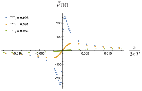
Figure 5: The normalized spectral function $\bar{\rho}_{\mathcal{O}^{\dagger}\mathcal{O}}(\omega)$ versus real $\omega/(2\pi T)$ for $Q=1/2$ and, from tallest to shortest, $T/T_{c}=0.998$ (blue), $0.991$ (orange), and $0.964$ (green).

Fig. 6 shows our numerical results for the position of $\omega_{p}$ versus small $\frac{\lambda_{K}^{2}}{N^{2}}\langle\mathcal{O}\rangle^{2}/(2\pi T)$, or equivalently, $T$ just below $T_{c}$, $T\lesssim T_{c}$, for $Q=1/2$. Fig. 6 also shows a linear fit demonstrating that

$$\omega_{p}\propto-i\left\langle{\cal O}\right\rangle^{2}.$$ (4)

Our model’s mean-field behavior $\langle\mathcal{O}\rangle\propto(T_{c}-T)^{1/2}$ then implies $\Gamma\propto T_{c}-T$ for $T\lesssim T_{c}$.

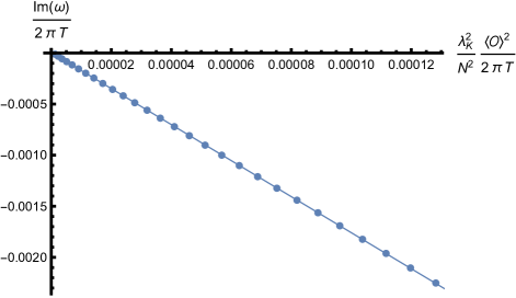
Figure 6: Dots denote the position of $G_{\mathcal{O}^{\dagger}\mathcal{O}}(\omega)$’s lowest pole versus $\frac{\lambda_{K}^{2}}{N^{2}}\langle\mathcal{O}\rangle^{2}/(2\pi T)$ for $Q=1/2$. The solid line is a linear fit with slope $\approx-17.6$ and intercept at the origin.

The behavior in (4) is in fact identical to that in a LFL at large $N$. In a LFL, the Kondo resonance is formally defined in the LFL fermion spectral function, and at large $N$ appears only in the screened phase, with $\Gamma\propto\langle\mathcal{O}\rangle^{2}$ Coleman (2015). For $T\lesssim T_{c}$, the mean-field behavior $\langle\mathcal{O}\rangle\propto(T_{c}-T)^{1/2}$ then implies $\Gamma\propto T_{c}-T$. Crucially, in the screened phase the Kondo resonance also appears in other spectral functions, due to operator mixing induced by the symmetry breaking Coleman (2015). In particular, a Kondo resonance should produce a pole in $G_{\mathcal{O}^{\dagger}\mathcal{O}}(\omega)$ precisely of the form in (4). Our result (4) thus proves the existence of a Kondo resonance in our model when $T\lesssim T_{c}$, with defining features essentially intact despite the strong interactions.

V Conclusion

In a holographic model describing the interaction of a magnetic impurity with a strongly correlated CFT at large $N$, we discovered a novel mechanism for producing Fano resonances, namely via RG flows between $(0+1)$-dimensional fixed points. The origin and consequences of such Fano resonances, in existing cases that have gone unidentified and in novel cases, deserve further study, particularly of the physics contained in the asymmetry parameter $q$.

References

- Kondo (1964) J. Kondo, Prog. Theo. Phys. 32, 37 (1964).
- Hewson (1993) A. Hewson, Cambridge University Press (1993).
- Cox and Zawadowski (1998) D. L. Cox and A. Zawadowski, Advances in Physics 47, 599 (1998), arxiv:cond-mat/9704103 .
- Lee and Toner (1992) D.-H. Lee and J. Toner, Phys. Rev. Lett. 69, 3378 (1992).
- Furusaki and Nagaosa (1994) A. Furusaki and N. Nagaosa, Phys. Rev. Lett. 72, 892 (1994).
- Fröjdh and Johannesson (1995) P. Fröjdh and H. Johannesson, Phys. Rev. Lett. 75, 300 (1995).
- Fröjdh and Johannesson (1996) P. Fröjdh and H. Johannesson, Phys. Rev. B 53, 3211 (1996).
- Furusaki (2005) A. Furusaki, Journal of the Physical Society of Japan 74, 73 (2005), cond-mat/0409016 .
- Fulde et al. (1993) P. Fulde, V. Zevin, and G. Zwicknagl, Zeitschrift für Physik B Condensed Matter 92, 133 (1993).
- Schork and Fulde (1994) T. Schork and P. Fulde, Phys. Rev. B 50, 1345 (1994), cond-mat/9402106 .
- Khaliullin and Fulde (1995) G. Khaliullin and P. Fulde, Phys. Rev. B 52, 9514 (1995).
- Igarashi et al. (1995) J. Igarashi, K. Murayama, and P. Fulde, Phys. Rev. B 52, 15966 (1995).
- Tornow et al. (1997) S. Tornow, V. Zevin, and G. Zwicknagl, eprint arXiv:cond-mat/9701137 (1997), cond-mat/9701137 .
- Schork and Blawid (1997) T. Schork and S. Blawid, Phys. Rev. B 56, 6559 (1997), cond-mat/9706225 .
- Davidovich and Zevin (1998) B. Davidovich and V. Zevin, Phys. Rev. B 57, 7773 (1998), cond-mat/9706283 .
- Duc and Thang (1999) H. T. Duc and N. T. Thang, Modern Physics Letters B 13, 849 (1999).
- Hofstetter et al. (2000) W. Hofstetter, R. Bulla, and D. Vollhardt, Physical Review Letters 84, 4417 (2000), cond-mat/9912396 .
- Erdmenger et al. (2013) J. Erdmenger, C. Hoyos, A. O’Bannon, and J. Wu, JHEP 12, 086 (2013), arXiv:1310.3271 [hep-th] .
- O’Bannon et al. (2016) A. O’Bannon, I. Papadimitriou, and J. Probst, JHEP 01, 103 (2016), arXiv:1510.08123 [hep-th] .
- Erdmenger et al. (2016) J. Erdmenger, M. Flory, C. Hoyos, M.-N. Newrzella, and J. M. S. Wu, Fortsch. Phys. 64, 109 (2016), arXiv:1511.03666 [hep-th] .
- Erdmenger et al. (2015) J. Erdmenger, M. Flory, C. Hoyos, M.-N. Newrzella, A. O’Bannon, and J. Wu, in The String Theory Universe, 21st European String Workshop and 3rd COST MP1210 Meeting Leuven, Belgium, September 7-11, 2015 (2015) arXiv:1511.09362 [hep-th] .
- Phillips (2012) P. Phillips, Cambridge University Press (2012).
- Coleman (2015) P. Coleman, Cambridge University Press (2015).
- Coleman and Andrei (1986) P. Coleman and N. Andrei, Jour. Phys. C19, 3211 (1986).
- Coleman (1987) P. Coleman, Phys. Rev. B35, 5072 (1987).
- Senthil et al. (2003) T. Senthil, S. Sachdev, and M. Vojta, Phys. Rev. Lett. 90, 216403 (2003), arXiv:cond-mat/0209144 .
- Senthil et al. (2004) T. Senthil, M. Vojta, and S. Sachdev, Phys. Rev. B69, 035111 (2004), arxiv:cond-mat/0305193 .
- Fano (1961) U. Fano, Phys. Rev. 124, 1866 (1961).
- Miroshnichenko et al. (2010) A. E. Miroshnichenko, S. Flach, and Y. S. Kivshar, Rev. Mod. Phys. 82, 2257 (2010).
- Madhavan et al. (1998) V. Madhavan, W. Chen, T. Jamneala, M. F. Crommie, and N. S. Wingreen, Science 280, 567 (1998).
- Madhavan et al. (2001) V. Madhavan, W. Chen, T. Jamneala, M. F. Crommie, and N. S. Wingreen, Phys. Rev. B 64, 165412 (2001).
- Göres et al. (2000) J. Göres, D. Goldhaber-Gordon, S. Heemeyer, M. A. Kastner, H. Shtrikman, D. Mahalu, and U. Meirav, Phys. Rev. B 62, 2188 (2000), cond-mat/9912419 .
- Parcollet et al. (1998) O. Parcollet, A. Georges, G. Kotliar, and A. Sengupta, Phys. Rev. B58, 3794 (1998), arXiv:cond-mat/9711192 .
- Faulkner et al. (2011a) T. Faulkner, H. Liu, J. McGreevy, and D. Vegh, Phys. Rev. D83, 125002 (2011a), arXiv:0907.2694 [hep-th] .
- Faulkner et al. (2011b) T. Faulkner, N. Iqbal, H. Liu, J. McGreevy, and D. Vegh, Phil. Trans. Roy. Soc. A 369, 1640 (2011b), arXiv:1101.0597 [hep-th] .
- Sachdev (2015) S. Sachdev, Phys. Rev. X5, 041025 (2015), arXiv:1506.05111 [hep-th] .
- Sachdev and Ye (1993) S. Sachdev and J.-W. Ye, Phys. Rev. Lett. 70, 3339 (1993), arXiv:cond-mat/9212030 [cond-mat] .
- Kitaev (2015) A. Kitaev, “A simple model of quantum holography,” (2015), talks for the KITP Strings seminar and Entanglement 2015 program, Feb. 12, Apr. 7, and May 27, 2015.
- Polchinski and Rosenhaus (2016) J. Polchinski and V. Rosenhaus, JHEP 04, 001 (2016), arXiv:1601.06768 [hep-th] .
- Jevicki et al. (2016) A. Jevicki, K. Suzuki, and J. Yoon, JHEP 07, 007 (2016), arXiv:1603.06246 [hep-th] .
- Maldacena and Stanford (2016) J. Maldacena and D. Stanford, Phys. Rev. D94, 106002 (2016), arXiv:1604.07818 [hep-th] .
- Jevicki and Suzuki (2016) A. Jevicki and K. Suzuki, JHEP 11, 046 (2016), arXiv:1608.07567 [hep-th] .
- Witten (2016) E. Witten, (2016), arXiv:1610.09758 [hep-th] .
- Erdmenger et al. (2017) J. Erdmenger, C. Hoyos, A. O’Bannon, I. Papadimitriou, J. Probst, and J. M. S. Wu, JHEP 03, 039 (2017), arXiv:1612.02005 [hep-th] .
- Affleck (1995) I. Affleck, Acta Phys. Polon. B26, 1869 (1995), arXiv:cond-mat/9512099 .
- Bickers, N. (1987) Bickers, N., Rev. Mod. Phys. 59, 845 (1987).
- Coleman (2007) P. Coleman, in Handbook of Magnetism and Advanced Magnetic Materials: Fundamentals and Theory, Vol. 1, edited by Kronmuller and Parkin (John Wiley and Sons, 2007) pp. 95–148, [arxiv:cond-mat/0612006] .
- Aharony et al. (2000) O. Aharony, S. S. Gubser, J. M. Maldacena, H. Ooguri, and Y. Oz, Phys. Rept. 323, 183 (2000), arXiv:hep-th/9905111 [hep-th] .
- Witten (2001) E. Witten, (2001), arXiv:hep-th/0112258 [hep-th] .
- Papadimitriou (2007) I. Papadimitriou, JHEP 0705, 075 (2007), arXiv:hep-th/0703152 [hep-th] .
- Son and Starinets (2002) D. T. Son and A. O. Starinets, JHEP 09, 042 (2002), arXiv:hep-th/0205051 .
- Kovtun and Starinets (2005) P. K. Kovtun and A. O. Starinets, Phys. Rev. D72, 086009 (2005), arXiv:hep-th/0506184 .