Lensing Constraints on the Mass Profile Shape and the Splashback Radius of Galaxy Clusters

Abstract

The lensing signal around galaxy clusters can, in principle, be used to test detailed predictions for their average mass profile from numerical simulations. However, the intrinsic shape of the profiles can be smeared out when a sample that spans a wide range of cluster masses is averaged in physical length units. This effect especially conceals rapid changes in gradient such as the steep drop associated with the splashback radius, a sharp edge corresponding to the outermost caustic in accreting halos. We optimize the extraction of such local features by scaling individual halo profiles to a number of spherical overdensity radii, and apply this method to 16 X-ray-selected high-mass clusters targeted in the Cluster Lensing And Supernova survey with Hubble. By forward-modeling the weak- and strong-lensing data presented by Umetsu et al., we show that, regardless of the scaling overdensity, the projected ensemble density profile is remarkably well described by a Navarro–Frenk–White (NFW) or Einasto profile out to $R\sim 2.5h^{-1}\,\mathrm{Mpc}$, beyond which the profiles flatten. We constrain the NFW concentration to $c_{\mathrm{200c}}=3.66\pm 0.11$ at $M_{\mathrm{200c}}\simeq 1.0\times 10^{15}h^{-1}\,M_{\odot}$, consistent with and improved from previous work that used conventionally stacked lensing profiles, and in excellent agreement with theoretical expectations. Assuming the profile form of Diemer & Kravtsov and generic priors calibrated from numerical simulations, we place a lower limit on the splashback radius of the cluster halos, if it exists, of $R_{\mathrm{sp}}^{\mathrm{3D}}/r_{\mathrm{200m}}>0.89$ ($R_{\mathrm{sp}}^{\mathrm{3D}}>1.83h^{-1}\,\mathrm{Mpc}$) at 68% confidence. The corresponding density feature is most pronounced when the cluster profiles are scaled by $r_{\mathrm{200m}}$, and smeared out when scaled to higher overdensities.

1. Introduction

Galaxy clusters, as the largest gravitationally bound objects formed in the universe, play a fundamental role in our understanding of cosmology and structure formation. A key ingredient for cluster-based cosmology is the distribution of dark matter (DM) in and around cluster halos. In this context, the standard $\Lambda$ cold dark matter ($\Lambda$CDM) model and its variants, such as self-interacting DM (SIDM, Spergel & Steinhardt, 2000) and wave DM ($\psi$DM, Schive et al., 2014), provide distinct, observationally testable predictions.

For the case of collisionless DM, high-resolution $N$-body simulations exhibit an approximately “universal” form for the spherically averaged density profile of halos in gravitational quasi-equilibrium (Navarro et al., 1997, hereafter NFW), $\rho(r)\propto(r/r_{\mathrm{s}})^{-1}(1+r/r_{\mathrm{s}})^{-2}$, where $r_{\mathrm{s}}$ is the characteristic scale radius at which the logarithmic density slope $d\ln{\rho}/d\ln{r}$ equals $-2$. In this context, the halo concentration, $c_{\mathrm{vir}}\equiv r_{\mathrm{vir}}/r_{\mathrm{s}}$, is a key quantity that characterizes the structure of a halo (all relevant symbols are defined in detail at the end of this section). In the hierarchical $\Lambda$CDM picture of structure formation, concentration is predicted to correlate with halo mass, $M_{\mathrm{vir}}$, because $r_{\mathrm{s}}$ stays nearly constant after an early phase of rapid accretion, whereas $r_{\mathrm{vir}}$ continues to grow through a mixture of physical accretion and pseudo-evolution (Bullock et al., 2001; Wechsler et al., 2002; Cuesta et al., 2008; Zhao et al., 2009; Diemer et al., 2013). As cluster halos are, on average, still actively growing today, they are expected to have relatively low concentrations, $c_{\mathrm{vir}}\sim 4$–$5$ (Bhattacharya et al., 2013; Dutton & Macciò, 2014; Diemer & Kravtsov, 2015). These general trends are complicated by the large scatter in halo growth histories, which translates into a significant diversity in their density profiles (Ludlow et al., 2013).

Recently, closer examination of the outer halo density profiles in collisionless $\Lambda$CDM simulations has revealed systematic deviations from the universal NFW or Einasto (1965) form (Diemer & Kravtsov, 2014, hereafter DK14). In particular, the profiles exhibit a sharp drop in density, a feature associated with the last shell that has reached the apocenter of its first orbit after accreting onto a halo in spherical collapse models (Gunn & Gott, 1972; Fillmore & Goldreich, 1984; Bertschinger, 1985). The location of this “splashback radius,” $R_{\mathrm{sp}}^{\mathrm{3D}}$, is within a factor of two of $r_{\mathrm{200m}}$ and depends on the mass accretion rate of halos, with a secondary dependence on redshift (Diemer & Kravtsov, 2014; Adhikari et al., 2014; More et al., 2015; Shi, 2016; More et al., 2016; Adhikari et al., 2016; Mansfield et al., 2016). The splashback radius constitutes a physically motivated halo boundary because (at least in the spherical case) material outside $R_{\mathrm{sp}}^{\mathrm{3D}}$ is on its first infall into the halo, whereas material inside of it is orbiting in the halo potential.

More et al. (2016) first observed the splashback feature in stacked galaxy surface density profiles around clusters (see also Tully 2015; Patej & Loeb 2016). Their measured $R_{\mathrm{sp}}^{\mathrm{3D}}$ is somewhat smaller than expected from the numerical calibration of More et al. (2015). This intriguing disagreement could be due to subtle effects in the analysis, errors in the numerical calculation, baryonic physics affecting cluster member galaxies, or hitherto undetected properties of the DM itself, such as self-interaction.

Given this wide range of possible reasons for the disagreement, other observational probes are of great interest. In particular, we are looking for a test that is subject to different systematic uncertainties than cluster member density profiles, but is still applicable to high-mass galaxy clusters where the splashback signal is expected to be strongest (Diemer & Kravtsov, 2014; Adhikari et al., 2014). One potential probe that fulfills these requirements is gravitational lensing, because it measures the total mass profile rather than the distribution of subhalos, while the signal is strongest in galaxy clusters.

Cluster gravitational lensing offers a well-established method for testing halo structure, through observations of weak shear lensing (e.g., von der Linden et al., 2014; Applegate et al., 2014; Gruen et al., 2014; Umetsu et al., 2014; Hoekstra et al., 2015; Okabe & Smith, 2016; Melchior et al., 2016), weak magnification lensing (e.g., Hildebrandt et al., 2011; Umetsu et al., 2011b; Coupon et al., 2013; Ford et al., 2014; Jimeno et al., 2015; Chiu et al., 2016; Ziparo et al., 2016), strong gravitational lensing (e.g., Broadhurst et al., 2005b; Zitrin et al., 2009; Coe et al., 2010; Jauzac et al., 2014; Diego et al., 2015), and the combination of all these effects (e.g., Broadhurst et al., 2005a; Umetsu & Broadhurst, 2008; Umetsu et al., 2011a, 2012, 2015, 2016; Coe et al., 2012; Medezinski et al., 2013). Over the last decade, cluster lensing observations (Broadhurst et al., 2005a; Okabe et al., 2010, 2013; Umetsu et al., 2011a, 2016; Newman et al., 2013) have established that the projected total mass distribution within individual and stacked clusters is well described by a family of density profiles predicted for cuspy DM-dominated halos, such as the NFW (Navarro et al., 1997), Einasto (Einasto, 1965), and DARKexp (Hjorth & Williams, 2010; Williams & Hjorth, 2010) models. Subsequent systematic studies targeting lensing-unbiased cluster samples (e.g., Okabe et al., 2013; Umetsu et al., 2014, 2016; Merten et al., 2015; Du et al., 2015) show that the cluster lensing measurements are also in agreement with the theoretical $c$–$M$ relation that is calibrated for recent $\Lambda$CDM cosmologies with a relatively high normalization (Bhattacharya et al., 2013; Dutton & Macciò, 2014; Meneghetti et al., 2014; Diemer & Kravtsov, 2015).

In principle, any feature in the density profiles predicted by numerical simulations is directly accessible by lensing observations of a large sample of galaxy clusters (e.g., Okabe et al., 2010, 2013; Umetsu et al., 2014, 2016; Miyatake et al., 2016). In reality, however, two effects make such measurements difficult. First, projecting the density profile into two dimensions smooths out features because any given sightline crosses a range of three-dimensional cluster radii. Second, in order to average lensing observations of individual clusters, we need to stack their density profiles using some radial scale. Conventionally, physical length units are chosen for this rescaling (e.g., Okabe et al., 2010; Sereno et al., 2015). If the cluster sample spans a wide range of masses, such a stacking procedure is likely to smooth out the intrinsic density profiles of the clusters, and sharp features such as the splashback radius in particular. Instead, we wish to rescale the profiles by a halo radius in units of which the features we are interested in are universal, i.e. they appear at the same rescaled radius. Numerical simulations show that this choice of scaling radius is far from trivial: while the inner profiles ($r\lower 2.15277pt\hbox{$\;\buildrel<\over{\sim}\;$}r_{\mathrm{vir}}$) are most universal with halo radii that scale with the critical density of the universe (such as $r_{\mathrm{200c}}$), the outer profiles are most universal when expressed in units of radii that scale with the mean cosmic density, such as $r_{\mathrm{200m}}$ (Diemer & Kravtsov, 2014; Lau et al., 2015). These predictions have not hitherto been tested observationally.

In this paper, we develop new methods for scaling and modeling stacked cluster lensing profiles, and undertake the first investigation of the splashback radius based on lensing observations. We use the data presented in Umetsu et al. (2016, hereafter U16), who performed a joint analysis of strong-lensing, weak-lensing shear and magnification data sets for 20 high-mass clusters targeted in the Cluster Lensing And Supernova survey with Hubble (CLASH, Postman et al., 2012; Umetsu et al., 2014, 2016; Zitrin et al., 2015; Merten et al., 2015). Their analysis combines constraints from 16-band Hubble Space Telescope (HST) observations and wide-field multicolor imaging taken primarily with Suprime-Cam on the Subaru telescope. Such a joint analysis of multiple lensing probes allows us not only to improve the precision of mass reconstructions, but also to calibrate systematic errors inherent in each probe (Rozo & Schmidt, 2010; Umetsu, 2013). The large radial range covered by the combination of weak- and strong-lensing data allows us to explore a range of scaling overdensities, and to investigate their impact on the stacked ensemble fit. Thanks to the improved stacking procedure, we derive tighter constraints on halo concentration than in U16, and put a lower limit on the splashback radius of the stacked CLASH density profile.

The paper is organized as follows. In Section 2 we summarize the characteristics of the CLASH sample and describe the data used in this study. We then outline our procedure for modeling the cluster lensing profiles, and test its robustness using synthetic CLASH weak-lensing data. In Section 3 we apply our methodology to the CLASH lensing data and fit them with NFW, Einasto, and DK14 profiles. We discuss the results in Section 4. Finally, a summary is given in Section 5.

Throughout this paper, we adopt a spatially flat $\Lambda$CDM cosmology with $\Omega_{\mathrm{m}}=0.27$, $\Omega_{\Lambda}=0.73$, and a Hubble constant $H_{0}=100h$ km s^-1 Mpc^-1 with $h=0.7$. We denote the mean matter density of the universe as $\rho_{\mathrm{m}}$ and the critical density as $\rho_{\mathrm{c}}$. We use the standard notation $M_{\Delta_{\mathrm{c}}}$ or $M_{\Delta_{\mathrm{m}}}$ to denote the mass enclosed within a sphere of radius $r_{\Delta_{\mathrm{c}}}$ or $r_{\Delta_{\mathrm{m}}}$, within which the mean overdensity equals $\Delta_{\mathrm{c}}\times\rho_{\mathrm{c}}(z)$ or $\Delta_{\mathrm{m}}\times\rho_{\mathrm{m}}(z)$ at a particular redshift $z$, such that $M_{\Delta\mathrm{c}}=(4\pi/3)\Delta_{\mathrm{c}}\rho_{\mathrm{c}}(z)r_{\Delta\mathrm{c}}^{3}$ and $M_{\Delta\mathrm{m}}=(4\pi/3)\Delta_{\mathrm{m}}\rho_{\mathrm{m}}(z)r_{\Delta\mathrm{m}}^{3}$. We generally denote three-dimensional cluster radii as $r$, and reserve the symbol $R$ for projected clustercentric distances. We define the splashback radius of a three-dimensional density profile, $R_{\mathrm{sp}}^{\mathrm{3D}}$, as the radius where the logarithmic slope of the profile is steepest. Similarly, we use $R_{\mathrm{sp}}^{\mathrm{2D}}$ to denote the splashback radius derived from the steepest slope of the projected profile. We compute the virial mass and radius, $M_{\mathrm{vir}}$ and $r_{\mathrm{vir}}$, using an expression for $\Delta_{\mathrm{vir}}(z)$ based on the spherical collapse model (Appendix A of Kitayama et al., 1998). For a given overdensity $\Delta$, the concentration parameter is defined as $c_{\Delta}=r_{\Delta}/r_{\mathrm{s}}$. All quoted errors are $1\sigma$ confidence limits (CL) unless otherwise stated.

2. Data and Methodology

2.1. CLASH Sample and Data

Table 1 Properties of the Cluster Sample

Cluster	$z_{\mathrm{l}}$	$M_{\mathrm{2500c}}$	$c_{\mathrm{2500c}}$	$M_{\mathrm{500c}}$	$c_{\mathrm{500c}}$	$M_{\mathrm{vir}}$	$c_{\mathrm{vir}}$	$M_{\mathrm{200m}}$	$c_{\mathrm{200m}}$
		$(10^{14}M_{\odot}/h)$		$(10^{14}M_{\odot}/h)$		$(10^{14}M_{\odot}/h)$		$(10^{14}M_{\odot}/h)$
Abell 383	$0.187$	$1.95\pm 0.44$	$1.83\pm 0.65$	$4.11\pm 1.21$	$3.97\pm 1.24$	$6.59\pm 2.33$	$7.63\pm 2.22$	$7.24\pm 2.64$	$8.91\pm 2.55$
Abell 209	$0.206$	$2.06\pm 0.48$	$0.68\pm 0.19$	$6.75\pm 1.38$	$1.71\pm 0.40$	$13.72\pm 3.23$	$3.54\pm 0.73$	$15.65\pm 3.81$	$4.16\pm 0.84$
Abell 2261	$0.224$	$4.14\pm 0.72$	$1.03\pm 0.31$	$10.95\pm 2.13$	$2.43\pm 0.62$	$19.74\pm 4.81$	$4.82\pm 1.11$	$21.99\pm 5.56$	$5.60\pm 1.27$
RX J2129.7$+$0005	$0.234$	$1.45\pm 0.31$	$1.71\pm 0.59$	$3.14\pm 0.81$	$3.75\pm 1.12$	$5.05\pm 1.56$	$7.15\pm 1.98$	$5.51\pm 1.75$	$8.21\pm 2.25$
Abell 611	$0.288$	$2.89\pm 0.64$	$1.10\pm 0.42$	$7.51\pm 1.86$	$2.56\pm 0.82$	$13.26\pm 4.04$	$4.97\pm 1.45$	$14.54\pm 4.58$	$5.64\pm 1.62$
MS2137$-$2353	$0.313$	$1.73\pm 0.50$	$0.68\pm 0.42$	$5.80\pm 1.80$	$1.71\pm 0.87$	$11.88\pm 5.12$	$3.44\pm 1.56$	$13.24\pm 5.98$	$3.90\pm 1.74$
RX J1532.9$+$3021	$0.348$	$3.11\pm 0.74$	$0.98\pm 0.48$	$8.71\pm 2.54$	$2.32\pm 0.96$	$15.78\pm 6.15$	$4.48\pm 1.69$	$17.17\pm 6.94$	$5.01\pm 1.86$
RX J2248.7$-$4431	$0.352$	$2.45\pm 0.58$	$0.77\pm 0.26$	$7.47\pm 1.56$	$1.90\pm 0.53$	$14.21\pm 3.48$	$3.75\pm 0.93$	$15.57\pm 3.92$	$4.19\pm 1.02$
MACS J1115.9$+$0129	$0.352$	$2.87\pm 0.79$	$1.26\pm 0.69$	$7.36\pm 2.83$	$2.87\pm 1.36$	$12.61\pm 6.34$	$5.44\pm 2.35$	$13.61\pm 7.05$	$6.05\pm 2.59$
MACS J1931.8$-$2635	$0.363$	$1.28\pm 0.70$	$1.59\pm 0.99$	$2.92\pm 1.20$	$3.47\pm 1.94$	$4.93\pm 1.95$	$6.44\pm 3.36$	$5.31\pm 2.14$	$7.13\pm 3.69$
MACS J1720.3$+$3536	$0.391$	$2.75\pm 0.60$	$1.16\pm 0.46$	$6.97\pm 1.77$	$2.68\pm 0.90$	$11.93\pm 3.77$	$5.05\pm 1.55$	$12.81\pm 4.16$	$5.58\pm 1.69$
MACS J0429.6$-$0253	$0.399$	$2.00\pm 0.49$	$1.36\pm 0.60$	$4.80\pm 1.47$	$3.06\pm 1.17$	$7.95\pm 3.03$	$5.70\pm 2.00$	$8.49\pm 3.32$	$6.27\pm 2.18$
MACS J1206.2$-$0847	$0.440$	$3.24\pm 0.71$	$1.03\pm 0.39$	$8.57\pm 1.74$	$2.43\pm 0.77$	$14.94\pm 3.71$	$4.58\pm 1.33$	$15.97\pm 4.07$	$5.00\pm 1.43$
MACS J0329.7$-$0211	$0.450$	$2.31\pm 0.45$	$2.12\pm 0.59$	$4.55\pm 0.96$	$4.53\pm 1.12$	$6.81\pm 1.61$	$8.11\pm 1.89$	$7.15\pm 1.72$	$8.79\pm 2.03$
RX J1347.5$-$1145	$0.451$	$5.35\pm 1.14$	$0.85\pm 0.31$	$15.63\pm 3.42$	$2.07\pm 0.62$	$28.46\pm 7.79$	$3.95\pm 1.06$	$30.51\pm 8.57$	$4.31\pm 1.15$
MACS J0744.9$+$3927	$0.686$	$3.02\pm 0.72$	$0.95\pm 0.40$	$8.36\pm 1.97$	$2.27\pm 0.81$	$14.40\pm 4.19$	$4.11\pm 1.34$	$14.93\pm 4.40$	$4.30\pm 1.39$
Stacked ensemble	$0.337$	$2.64\pm 0.14$	$1.03\pm 0.10$	$6.87\pm 0.43$	$2.43\pm 0.20$	$11.99\pm 0.93$	$4.69\pm 0.35$	$13.03\pm 1.04$	$5.26\pm 0.38$

Note. — All mass estimates listed are based on the combined strong-lensing, weak-lensing shear and magnification analysis of Umetsu et al. (2016). See Table 2 of Umetsu et al. (2016) for $M_{\mathrm{200c}}$ and $c_{\mathrm{200c}}$. The effective $M_{\Delta}$ masses of the sample were extracted from a spherical NFW fit to their stacked surface mass density profile (Umetsu et al., 2016). The best-fit model yields $M_{\mathrm{200c}}=(10.11\pm 0.73)\times 10^{14}M_{\odot}\,h^{-1}$ and $c_{\mathrm{200c}}=3.76\pm 0.28$ (symmetrized errors; see the NFW model in Table 4 of Umetsu et al., 2016). The effective redshift of the sample represents a sensitivity-weighted average of their redshifts (Section 5.4 of Umetsu et al., 2016), $0.337$, which is close to the median redshift, $\overline{z}_{\mathrm{l}}=0.352$.

The CLASH survey (Postman et al., 2012) is a 524-orbit HST Multi-Cycle Treasury program targeting 25 high-mass galaxy clusters. Of these, 20 CLASH clusters were selected to be X-ray hot ($T_{X}>5$ keV) and to have a high degree of regularity in their X-ray morphology, with no lensing information used a priori. Another subset of five clusters were selected by their high-magnification properties. These high-magnification clusters often turn out to be complex, massive merging systems (e.g., Zitrin et al., 2013; Medezinski et al., 2013). A complete definition of the CLASH sample is given in Postman et al. (2012).

In this work, we shall focus on the analysis of the X-ray-selected subsample to simplify the interpretation of our results. Numerical simulations suggest that this subsample is mostly composed of relaxed clusters ($\sim 70\%$) and largely free of orientation bias (Meneghetti et al., 2014). Specifically, we use a lensing-unbiased subset of 16 CLASH X-ray-selected clusters taken from U16, who performed a comprehensive analysis of the strong-lensing, weak-lensing shear and magnification data. Our cluster sample lies in the redshift range $0.19\lower 2.15277pt\hbox{$\;\buildrel<\over{\sim}\;$}z_{\mathrm{l}}\lower 2.15277pt\hbox{$\;\buildrel<\over{\sim}\;$}0.69$ and over a mass range $5\lower 2.15277pt\hbox{$\;\buildrel<\over{\sim}\;$}M_{\mathrm{vir}}/(10^{14}h^{-1}\,M_{\odot})\lower 2.15277pt\hbox{$\;\buildrel<\over{\sim}\;$}30$ (Table 1), spanning a factor of $\sim 6$ in halo mass $M_{\Delta}$, or a factor of $\sim 1.8$ in $r_{\Delta}\propto M_{\Delta}^{1/3}$. A full description of the data used in this work is given by U16. Here, we provide only a brief summary of the most relevant aspects of the lensing reconstructions.

The U16 analysis uses the cluster lensing mass inversion (clumi) code developed by Umetsu et al. (2011b) and Umetsu (2013), in which lensing constraints are combined a posteriori in the form of azimuthally averaged radial profiles. U16 used constraints spanning the radial range $10\arcsec$–$960\arcsec$ obtained from 16-band HST observations (Zitrin et al., 2015) and wide-field multicolor imaging (Umetsu et al., 2014) taken primarily with Subaru/Suprime-Cam. The position of the brightest cluster galaxy (BCG) is adopted as the cluster center (Table 1 in U16). Umetsu et al. (2014) obtained weak-lensing shear and magnification measurements in 10 logarithmically spaced radial bins ($N_{\mathrm{WL}}=10$) over the range $0.9\arcmin$–$16\arcmin$ for all clusters observed with Subaru, and $0.9\arcmin$–$14\arcmin$ for RX J2248.7$-$4431 observed with ESO/WFI. Zitrin et al. (2015) constructed detailed mass models for each cluster core from a joint analysis of HST strong and weak-shear lensing data. U16 constructed enclosed projected mass constraints for a set of four equally-spaced integration radii ($10\arcsec$–$40\arcsec$, $N_{\mathrm{SL}}=4$) from the HST lensing analysis of Zitrin et al. (2015). U16 combined these full lensing constraints for individual clusters in their joint likelihood analysis to reconstruct binned surface mass density profiles $\mbox{\boldmath$\Sigma$}=\{\Sigma(R_{i})\}_{i=1}^{N_{\mathrm{bin}}}$ measured in a set of clustercentric radial bins, $\mbox{\boldmath$R$}=\{R_{i}\}_{i=1}^{N_{\mathrm{bin}}}$ with $N_{\mathrm{bin}}=N_{\mathrm{SL}}+N_{\mathrm{WL}}+1$. We have $N_{\mathrm{bin}}=15$ bins for all clusters, except $N_{\mathrm{bin}}=11$ for RX J1532.9$+$3021 with $N_{\mathrm{SL}}=0$, for which no secure identification of multiple images was made (Zitrin et al., 2015). The $\Sigma$ profiles used in this work are shown in Figure 11 of U16.

U16 accounted for various sources of errors. Their analysis includes four terms in the total covariance matrix $C_{ij}$ of the $\Sigma$ profile,

$$C=C^{\mathrm{stat}}+C^{\mathrm{sys}}+C^{\mathrm{lss}}+C^{\mathrm{int}},$$ (1)

where $C^{\mathrm{stat}}$ represents statistical observational errors, $C^{\mathrm{sys}}$ contains systematic uncertainties due primarily to the residual mass-sheet uncertainty (Umetsu et al., 2014), $C^{\mathrm{lss}}$ is the cosmic-noise covariance matrix due to projected uncorrelated large-scale structures (Hoekstra, 2003; Umetsu et al., 2011a), and $C^{\mathrm{int}}$ accounts for the intrinsic variations of the projected cluster lensing signal at fixed mass due to variations in halo concentration, cluster asphericity, and the presence of correlated halos (Gruen et al., 2015). Overall, the reconstruction uncertainty is dominated by the $C^{\mathrm{stat}}$ term (Figure 1 of U16). The relative contribution from the $C^{\mathrm{int}}$ term becomes increasingly dominant at small cluster radii, especially at $\theta\lower 2.15277pt\hbox{$\;\buildrel<\over{\sim}\;$}2\arcmin$. The impact of the $C^{\mathrm{lss}}$ term is most important at large cluster radii, where the cluster signal is small.

Table 1 summarizes CLASH lensing determinations of the mass and concentration parameters $(M_{\Delta},c_{\Delta})$ for our 16 clusters based on the full lensing analysis of U16. These values were obtained from spherical NFW fits to individual cluster $\Sigma$ profiles using the total covariance matrix $C$ (Equation (1)), restricting the fitting range to $R\leq 2h^{-1}\,\mathrm{Mpc}$ ($\sim 2r_{\mathrm{500c}}\sim r_{\mathrm{200m}}$ for the CLASH sample) to avoid systematic effects (Becker & Kravtsov, 2011; Meneghetti et al., 2014). In Table 1, we also list effective overdensity masses $M_{\Delta}^{\mathrm{eff}}$ of the sample, which were obtained by U16 from a spherical NFW fit to the stacked surface mass density profile of the 16 CLASH clusters. The stacked ensemble has an effective halo mass $M_{\mathrm{vir}}^{\mathrm{eff}}=(11.99\pm 0.93)\times 10^{14}h^{-1}\,M_{\odot}$ and an effective halo concentration $c_{\mathrm{vir}}^{\mathrm{eff}}=4.69\pm 0.35$ ($c_{\mathrm{200c}}^{\mathrm{eff}}=3.76\pm 0.28$; see Table 1), and lies at a sensitivity-weighted average redshift of $z_{\mathrm{l}}^{\mathrm{eff}}=0.337$, close to the median redshift of $\overline{z}_{\mathrm{l}}=0.352$.

U16 quantified potential sources of systematic uncertainty in their mass calibration (see their Section 7.1), such as the effect of dilution of the weak-lensing signal by cluster members (2.4%), photometric-redshift bias (0.27%), shear calibration uncertainty (5%), and projection effects of prolate halos (3%). Combining them in quadrature, the total systematic uncertainty in the absolute mass calibration was estimated to be $\simeq 6\%$. This is in close agreement with the value $\sim 8\%$ empirically estimated from the shear-magnification consistency test of Umetsu et al. (2014).

Another potential source of systematic errors is smoothing of the central lensing signal from miscentering effects (Johnston et al., 2007; Umetsu et al., 2011a; Du & Fan, 2014). On average, the sample exhibits a small positional offset between the BCG and the X-ray peak, characterized by an rms offset of $\sigma_{\mathrm{off}}\simeq 11h^{-1}\,\mathrm{kpc}$ (Umetsu et al., 2014, 2016), which is much smaller than the typical resolution limit of our HST lensing data ($\theta_{\mathrm{min}}=10\arcsec$, corresponding to $\simeq 35h^{-1}\,\mathrm{kpc}$ at $\overline{z}_{\mathrm{l}}=0.35$). Hence, the miscentering effects are not expected to significantly affect our ensemble lensing analysis.

2.2. Radial Scaling of the Profiles

One of our main goals in this work is to investigate how the radial scaling of stacked profiles influences the fit results. Ideally, one would like to stack profiles as a function of the exact halo radius where a particular feature is expected, e.g. the NFW scale radius or the splashback radius. However, since their locations are a priori unknown, we need to resort to an alternative halo radius that can be measured for individual clusters, generally a spherical overdensity radius $r_{\Delta}$. Now, the goal is to choose a definition in which the location of the feature in question is universal, i.e. independent of halo mass, and possibly of redshift.

Unfortunately, there is no guarantee that any one definition will be ideal for multiple features. In fact, DK14 discovered that halo density profiles in $N$-body simulations prefer different scaling radii in different regions of the profile: while the inner profiles (and thus concentrations) are most universal when expressed in units of halo radii that scale with the critical density $\rho_{\mathrm{c}}(z)$ of the universe, such as $r_{\mathrm{200c}}$, the outer profiles (and thus the splashback radius) are most universal in units of halo radii that scale with the mean cosmic density $\rho_{\mathrm{m}}(z)$, such as $r_{\mathrm{200m}}$. These scalings were confirmed in hydrodynamical simulations of galaxy clusters (Lau et al., 2015, see also Shi 2016). As we wish to investigate both the inner and outer profiles, we repeat our analysis using a number of different scalings covering a range between $2500\rho_{\mathrm{c}}$ and $200\rho_{\mathrm{m}}\simeq 94\rho_{\mathrm{c}}$ at $z_{\mathrm{l}}^{\mathrm{eff}}=0.337$.

To construct the scaled surface mass density profiles for the CLASH sample, we use our full lensing constraints on the NFW parameters $M_{\Delta}$ and $c_{\Delta}$ of each individual cluster as obtained by U16 (Section 2.1; see Table 1), and normalize their observed $\Sigma(R)$ profiles to a given overdensity $\Delta$ of interest. We stress that we do not rely on scaling relations (e.g., the $c$–$M$ relation), but use observational lensing constraints on $r_{\Delta}$ and $\Sigma(r_{\Delta})$ for each cluster. The high-quality, multiscale weak- and strong-lensing constraints from the CLASH survey enable us to explore the wide range of overdensities listed above.

We choose the NFW model for the scaling because recent cluster lensing observations show that the “projected total” matter distribution in the intracluster region ($R\lower 2.15277pt\hbox{$\;\buildrel<\over{\sim}\;$}r_{\mathrm{200m}}$) is in excellent agreement with the NFW form (Umetsu et al., 2011a, 2014, 2016; Beraldo e Silva et al., 2013; Newman et al., 2013; Okabe et al., 2013; Niikura et al., 2015; Okabe & Smith, 2016), as predicted for collisionless DM-dominated halos in $N$-body cosmological simulations (Oguri & Hamana, 2011; Meneghetti et al., 2014). We demonstrate the consistency of this choice with our results in Section 3.

2.3. Fitting Functions

The second goal of this work (besides investigating radial scalings) is to constrain the splashback radius of the CLASH cluster sample. While NFW and Einasto fitting functions were sufficient for the radial rescaling, they describe only the 1-halo term and do not take the steepening due to the splashback radius into account. Thus, we also fit the cluster lensing profiles with the more flexible fitting function of DK14 which was calibrated to a suite of $\Lambda$CDM $N$-body simulations. We emphasize that the quality of the data is insufficient to distinguish among the different profile models, which all describe the data very well (see Section 3.1). Nevertheless, in order to constrain the location of the splashback radius, we assume that the $\Lambda$CDM simulations of DK14 describe real cluster halos and use the DK14 profile as a fitting function in conjunction with generic priors.

Furthermore, we note that the “true” location of the splashback radius is not strictly equivalent to a particular location in the spherically averaged density profile. However, we follow More et al. (2015) in defining $R_{\mathrm{sp}}^{\mathrm{3D}}$ as the radius where the logarithmic slope of the three-dimensional density profile is steepest. According to this definition, $R_{\mathrm{sp}}^{\mathrm{3D}}$ is expected to lie within a factor of two of $r_{\mathrm{200m}}$ (More et al., 2015). Furthermore, the steepest slope would need to be steeper than that expected from the sum of the Einasto profile and the 2-halo term at large scales if a detection were to be claimed (More et al., 2016).

The DK14 fitting formula is described by eight parameters, and is sufficiently flexible to reproduce a range of fitting functions for the DM density profile, such as the halo model (Oguri & Hamana, 2011; Hikage et al., 2013). We use the publicly available code colossus (Diemer, 2015) for many of calculations relating to density profiles. The DK14 model is given by

$$\Delta\rho(r) =\rho(r)-\rho_{\mathrm{m}}=\rho_{\mathrm{inner}}\times f_{\mathrm{trans}}+\rho_{\mathrm{outer}},$$ (2)

$$\rho_{\mathrm{inner}} =\rho_{\mathrm{Einasto}}=\rho_{\mathrm{s}}\exp\left\{-\frac{2}{\alpha}\left[\left(\frac{r}{r_{\mathrm{s}}}\right)^{\alpha}-1\right]\right\},$$

$$f_{\mathrm{trans}} =\left[1+\left(\frac{r}{r_{\mathrm{t}}}\right)^{\beta}\right]^{-\frac{\gamma}{\beta}},$$

$$\rho_{\mathrm{outer}} =\frac{b_{\mathrm{e}}\rho_{\mathrm{m}}}{\Delta_{\mathrm{max}}^{-1}+(r/r_{\mathrm{piv}})^{s_{\mathrm{e}}}},$$

with $r_{\mathrm{piv}}=5r_{\mathrm{200m}}$ and $\Delta_{\mathrm{max}}=10^{3}$. Here $\Delta_{\mathrm{max}}$ has been introduced as a maximum cutoff density of the outer term to avoid a spurious contribution at small halo radii (Diemer, 2015). The Einasto profile $\rho_{\mathrm{Einasto}}$ describes the intracluster mass distribution, with the shape parameter $\alpha$ describing the degree of profile curvature and $r_{\mathrm{s}}$ the scale radius at which the logarithmic slope is -2. The transition term $f_{\mathrm{trans}}$ characterizes the steepening around a truncation radius, $r_{\mathrm{t}}$. The outer term $\rho_{\mathrm{outer}}$, given by a softened power law, is responsible for the correlated matter distribution around clusters, also known as the 2-halo term, $\rho_{\mathrm{2h}}$. DK14 found that this fitting function provides a precise description ($\lower 2.15277pt\hbox{$\;\buildrel<\over{\sim}\;$}5\%$) of their simulated DM density profiles at $r\lower 2.15277pt\hbox{$\;\buildrel<\over{\sim}\;$}9r_{\mathrm{vir}}$. At larger radii, the outer term is expected to follow a shape proportional to the matter correlation function (e.g., Oguri & Takada, 2011).

To scale out the mass dependence of the density profile, we use an arbitrary overdensity radius $r_{\Delta}$ as a pivot radius, and define a scaled version of $\Delta\rho(r)$ as a function of $r=r_{\Delta}x$, namely

$$\Delta\rho(r)\propto \exp\left[-\frac{2}{\alpha}c_{\Delta}^{\alpha}(x^{\alpha}-1)\right]\left[1+\left(\frac{x}{\tau_{\Delta}}\right)^{\beta}\right]^{-\frac{\gamma}{\beta}}$$ (3)

$$+\frac{B_{\Delta}}{\epsilon_{\Delta}+x^{s_{\mathrm{e}}}}\equiv f_{\Delta}(x),$$

with $\epsilon_{\Delta}=\Delta_{\mathrm{max}}^{-1}\times(5r_{\mathrm{200m}}/r_{\Delta})^{s_{\mathrm{e}}}$. This scaled DK14 model is described by a set of seven dimensionless parameters,

$$\mbox{\boldmath$p$}=\{c_{\Delta},\alpha,\tau_{\Delta},B_{\Delta},s_{\mathrm{e}},\beta,\gamma\},$$ (4)

namely the halo concentration $c_{\Delta}=r_{\Delta}/r_{\mathrm{s}}$, the Einasto shape parameter $\alpha$, the dimensionless truncation radius $\tau_{\mathrm{\Delta}}=r_{\mathrm{t}}/r_{\mathrm{\Delta}}$, the relative normalization of the outer term $B_{\Delta}\propto b_{\mathrm{e}}$, and three additional shape parameters ($s_{\mathrm{e}},\beta,\gamma$) for the transition and outer terms. The model reduces to the Einasto model (specified by $c_{\Delta}$ and $\alpha$) when $f_{\mathrm{trans}}=1$ ($\tau_{\Delta}\to\infty$) and $f_{\mathrm{outer}}=0$ ($B_{\Delta}=0$). We refer the reader to Appendix A for a more detailed description of the scaled DK14 profile function. Similarly, we define a scaled version of the NFW profile, $\Delta\rho(r)\propto[c_{\Delta}x(1+c_{\Delta}x)^{2}]^{-1}$ with $r=r_{\Delta}x$, described by the concentration parameter $c_{\Delta}$.

By projecting $\Delta\rho(r)$ along the line of sight, we derive the scaled surface mass density, which is a lensing observable,

$$y_{\Delta}(x):=\frac{\Sigma(R=r_{\mathrm{\Delta}}x)}{\Sigma(r_{\mathrm{\Delta}})},$$ (5)

normalized as $y_{\Delta}(x)=1$ at $x=1$, where

$$\Sigma(R)=2\int_{R}^{\infty}\frac{\Delta\rho(r)rdr}{\sqrt{r^{2}-R^{2}}}.$$ (6)

The projected $y_{\Delta}(x)$ profile is modeled in terms of the scaled density profile $f_{\Delta}$ as

$$y_{\Delta}(x|\mbox{\boldmath$p$})=\left(\int_{x}^{\infty}\!\frac{f_{\Delta}(\xi|\mbox{\boldmath$p$})\xi d\xi}{\sqrt{\xi^{2}-x^{2}}}\right)\left(\int_{1}^{\infty}\!\frac{f_{\Delta}(\xi|\mbox{\boldmath$p$})\xi d\xi}{\sqrt{\xi^{2}-1}}\right)^{-1}.$$ (7)

We note that it is straightforward to generalize our approach to shear-only weak-lensing observations where the differential surface mass density $\Delta\Sigma(R)=\Sigma(<R)-\Sigma(R)$ is a direct observable in the weak-lensing limit (e.g., Bartelmann & Schneider, 2001).

2.4. Parameter Inference

We use a Bayesian approach to infer the shape and structural parameters of the mass distribution of the CLASH sample. We restrict the optimization to ($c_{\Delta},\alpha,\tau_{\Delta},B_{\Delta}$), the primary model parameters that describe the scaled DK14 model, and marginalize over the remaining parameters, $(s_{\mathrm{e}},\beta,\gamma)$, using priors based on the $N$-body simulations of DK14. In particular, following More et al. (2016), we adopt Gaussian priors of $\log_{10}\beta=\log_{10}{6}\pm 0.2$ and $\log_{10}\gamma=\log_{10}{4}\pm 0.2$, allowing a wide, representative range of values. We assume a Gaussian prior on $s_{\mathrm{e}}$ of $1.5\pm 0.1$, centered around the value found by DK14. We use unconstraining flat priors on $(c_{\Delta},\alpha,B_{\Delta})$. For $\tau_{\Delta}$, we assume $\tau_{\mathrm{200m}}\in[0,5]$, where the upper bound corresponds approximately to $r_{\mathrm{t}}=5r_{\mathrm{200m}}\simeq 10h^{-1}\,\mathrm{Mpc}$ for the CLASH sample (Table 1), which is larger than the maximum data radius of $\sim 5h^{-1}\,\mathrm{Mpc}$. We translate this prior to a given overdensity $\Delta$ using the effective $r_{\Delta}$ radius of the sample (Section 2.1 and Table 1) as $\tau_{\Delta}\in[0,5(r_{\mathrm{200m}}^{\mathrm{eff}}/r_{\Delta}^{\mathrm{eff}})]$.

We use a Gaussian log-likelihood $-\ln{\cal L}(\mbox{\boldmath$p$})=\chi^{2}(\mbox{\boldmath$p$})/2+\mathrm{const.}$ with a $\chi^{2}$ function given by

$$\chi^{2}=\sum_{n=1}^{N_{\mathrm{halo}}}\sum_{i,j=1}^{N_{\mathrm{bin}}} \left[y_{\Delta,i}^{(n)}-y_{\Delta}(x^{(n)}_{i}|\mbox{\boldmath$p$})\right]\left[C^{(n)}_{\Delta}\right]^{-1}_{ij}$$ (8)

$$\times \left[y_{\Delta,j}^{(n)}-y_{\Delta}(x^{(n)}_{j}|\mbox{\boldmath$p$})\right],$$

where $\mbox{\boldmath$y$}_{\Delta}=\{y_{\Delta,i}\}_{i=1}^{N_{\mathrm{bin}}}$ is the scaled data vector (see Equation (5)) for each cluster sampled at $\mbox{\boldmath$x$}=\{x_{i}\}_{i=1}^{N_{\mathrm{bin}}}=\{R_{i}/r_{\Delta}\}_{i=1}^{N_{\mathrm{bin}}}$, $C_{\Delta}$ is the total covariance matrix of the scaled data $\mbox{\boldmath$y$}_{\Delta}$, and $y_{\Delta}(x_{i}|\mbox{\boldmath$p$})$ represents the model for $y_{\Delta,i}$ with parameters $p$. Combining all 16 clusters in our sample, we have a total of $236$ data points (Section 2.1).

We use a Markov chain Monte Carlo (MCMC) approach with Metropolis–Hastings sampling to sample from the posterior distribution of the parameters, $(c_{\Delta},\alpha,\tau_{\Delta},B_{\Delta},s_{\mathrm{e}},\log_{10}\beta,\log_{10}\gamma)$, given the data and the priors stated above. We largely follow the sampling procedure of Dunkley et al. (2005) but employ the Gelman–Rubin statistic (Gelman & Rubin, 1992) as a convergence criterion of the generated chains. Once convergence to a stationary distribution is achieved, we run a long, final chain of $10^{5}$ sampled points, which is used for our parameter estimation and error analysis. We also use the minuit package from the CERN program libraries to find the global maximum a posteriori estimate of the joint probability distribution. This procedure allows a further refinement of the best-fit solution with respect to the one obtained from the MCMC sampling (see discussions in Planck Collaboration et al., 2014; Penna-Lima et al., 2016).

2.5. Tests with Synthetic Data

$\begin{array}[]{c@{\hspace{.3in}}c}\includegraphics[scale={0.45},angle={0},clip]{Figs/f1a.pdf}\hfil\hskip 21.68121pt&\includegraphics[scale={0.45},angle={0},clip]{Figs/f1b.pdf}\\ \includegraphics[scale={0.45},angle={0},clip]{Figs/f1c.pdf}\hfil\hskip 21.68121pt&\includegraphics[scale={0.45},angle={0},clip]{Figs/f1d.pdf}\end{array}$

Figure 1.— Test of our forward-modeling method. We create 50 realizations of CLASH-like weak-lensing data by computing synthetic shear and magnification catalogs from analytically modeled cluster lenses. We simulate two configurations of the outer density profile, one without a splashback feature (top panels) and one with a splashback-like feature (bottom panels, see Appendix B for details on the lens models). The left panels show the scaled surface mass density $\Sigma(R)/\Sigma(r_{\mathrm{200m}})$ of the synthetic observations, where the black solid line represents the noise-free, sensitivity-weighted profile of the 16 clusters in the synthetic sample. The blue shaded region indicates the $1\sigma$ bounds on the ensemble of DK14 fits to the synthetic data. The gray lines show scaled $\Sigma(R)$ profiles of individual clusters reconstructed from each particular source realization. The right panels show the logarithmic slope of the three-dimensional DK14 profiles, $d\ln\Delta\rho(r)/d\ln{r}$, as a function of $r/r_{\mathrm{200m}}$. For the lens model with a splashback-like feature, the range from the 16th to the 84th percentile of $R_{\mathrm{sp}}^{\mathrm{3D}}$ (gray vertical shaded area) inferred from the synthetic data is consistent with the sensitivity-weighted expectation value of the sample (red vertical line), $\langle R_{\mathrm{sp}}^{\mathrm{3D}}/r_{\mathrm{200m}}\rangle\simeq 0.87$. In each panel, the blue dotted lines indicate the errors scaled to match the overall CLASH weak-lensing sensitivity. This test demonstrates the robustness of our fitting method, and in particular that fitting the DK14 profile does not introduce a spurious splashback feature. See Section 2.5 and Appendix B for details.

Table 2 Best-fit NFW, Einasto, and DK14 parameters for the CLASH Sample

$\Delta$	NFW		Einasto			DK14
	$c_{\Delta}$	$\chi^{2}/\mathrm{dof}$	$c_{\Delta}$	$\alpha$	$\chi^{2}/\mathrm{dof}$	$c_{\Delta}$	$\alpha$	$\tau_{\Delta}$	$B_{\Delta}$	$\chi^{2}/\mathrm{dof}$
200m	$5.13\pm 2.9\%$	181/235	$4.57\pm 4.9\%$	$0.200\pm 9.3\%$	181/234	$4.96\pm 25\%$	$0.198\pm 28\%$	$>0.82$ ($1.13$)	$0.28\pm 0.41$	180/232
virial	$4.58\pm 2.9\%$	179/235	$4.08\pm 4.5\%$	$0.205\pm 9.6\%$	179/234	$4.43\pm 25\%$	$0.208\pm 26\%$	$>0.93$ ($1.40$)	$0.20\pm 0.37$	179/232
200c	$3.66\pm 3.1\%$	177/235	$3.30\pm 3.9\%$	$0.210\pm 11\%$	178/234	$3.58\pm 25\%$	$0.214\pm 26\%$	$>1.17$ ($1.75$)	$0.15\pm 0.31$	177/232
500c	$2.38\pm 3.5\%$	172/235	$2.19\pm 3.5\%$	$0.208\pm 13\%$	171/234	$2.43\pm 27\%$	$0.218\pm 25\%$	$>1.85$ ($2.92$)	$0.10\pm 0.20$	171/232
2500c	$1.05\pm 5.2\%$	153/235	$0.85\pm 14\%$	$0.174\pm 22\%$	151/234	$1.06\pm 33\%$	$0.182\pm 34\%$	$>3.12$ ($4.68$)	$0.15\pm 0.13$	151/232

Note. — The global best-fit parameters and their $1\sigma$ fractional errors (in per cent) for each model, with five different values of the scaling overdensity $\Delta$. For the DK14 parameter $B_{\Delta}$, we give the best-fit parameter and its $1\sigma$ uncertainty. For the DK14 parameter $\tau_{\Delta}$, we provide lower limits (68% CL) and best-fit parameter values in parentheses.

Given the simulation results of DK14, we expect the signature of the splashback radius in lensing data to be weak. Thus, one concern is that fitting with the DK14 profile function might introduce a spurious “detection” of a splashback feature due to systematics or overfitting in the presence of noise. In order to address this potential issue, we have tested our procedure (including data analysis, mass reconstruction, stacking, and the fitting process) on simulated lensing data. We focus on the recovery of the lensing signal in the noisy outer regions around $r_{\mathrm{200m}}$ where the splashback feature is expected. Hence, we consider only the wide-field weak-lensing observables, namely the shear and magnification effects in the subcritical regime. To this end, we create 50 source realizations of synthetic shear and magnification catalogs for our 16 CLASH clusters, each modeled as an NFW halo specified by its redshift $z_{\mathrm{l}}$ (Table 1) and ($M_{\mathrm{200c}},c_{\mathrm{200c}}$) parameters fixed to the observed central values (Table 2 of U16). For each NFW cluster, we consider two configurations of the outer density profile, one with and one without a splashback-like feature. For technical reasons, we do not use a DK14 profile for the synthetic cluster lenses and instead substitute a profile that introduces a similar density drop (see Appendix B for details).

The results of applying our methods to the synthetic weak-lensing data are summarized in Figure 1. The lower and upper panels correspond to the simulations with and without a splashback-like feature, respectively. The blue shaded region in the left panels shows the mean and standard deviation of the best-fit DK14 profiles inferred from 50 realizations of the synthetic data for each configuration. On average, this fit is in excellent agreement with the noise-free, sensitivity-weighted averaged input profile (black solid curve). In the right panels, we show the corresponding logarithmic density slope $d\ln\Delta\rho(r)/d\ln{r}$. For the model with a splashback-like feature, the range from the 16th to the 84th percentile of $R_{\mathrm{sp}}^{\mathrm{3D}}$ ($0.74\leq R_{\mathrm{sp}}^{\mathrm{3D}}/r_{\mathrm{200m}}\leq 1.27$; vertical shaded area) inferred from the synthetic data is consistent with the sensitivity-weighted expectation value of the sample, $\langle R_{\mathrm{sp}}^{\mathrm{3D}}/r_{\mathrm{200m}}\rangle\simeq 0.87$.

In Figure 1, we also indicate the errors scaled to the CLASH weak-lensing sensitivity (dotted lines). The errors are computed by matching the synthetic (NFW) to the observed (CLASH) total signal-to-noise ratio (S/N) of the $\Sigma$ profiles, where $(\mathrm{S/N})^{2}=\sum_{n=1}^{N_{\mathrm{halo}}}\left(\mbox{\boldmath$\Sigma$}^{t}C^{-1}\mbox{\boldmath$\Sigma$}\right)_{n}$. This comparison suggests that the overall uncertainty in our synthetic observations is underestimated by $\simeq 36\%$. Nevertheless, the $1\sigma$ uncertainty after this correction is small compared to the absolute value of the slope at $r\lower 2.15277pt\hbox{$\;\buildrel<\over{\sim}\;$}2r_{\mathrm{200m}}$. Even though the determination becomes noisy at radii around and beyond $r_{\mathrm{200m}}$, the steepening relative to the NFW profile is marginally identified at the $1.7\sigma$ level at the expected location, $r/r_{\mathrm{200m}}\sim 0.9$.

This test demonstrates that our analysis methods are able to accurately reproduce the input sensitivity-weighted density profile and its logarithmic gradient even at realistic noise levels. The results also show that the priors adopted (Section 2.4) are generic and flexible enough to reproduce the NFW-like shape of the profile, as well as a splashback feature. Importantly, we note that our analysis pipeline does not introduce spurious gradients that mimic the characteristic splashback feature, namely a steepening followed by an upturn due to the contribution from the 2-halo term.

$\begin{array}[]{c@{\hspace{.3in}}c}\includegraphics[scale={0.45},angle={0},clip]{Figs/f2a.pdf}\hfil\hskip 21.68121pt&\includegraphics[scale={0.45},angle={0},clip]{Figs/f2b.pdf}\end{array}$

Figure 2.— Upper panels: scaled surface mass density $\Sigma/\Sigma(r_{\Delta})$ of the CLASH sample as a function of $R/r_{\Delta}$, where the projected clustercentric distance $R$ is expressed in units of two different overdensity radii, $\Delta=\mathrm{200m}$ (left) and $\mathrm{2500c}$ (right). In each panel, the blue thick solid line and the blue shaded area show the best-fit DK14 profile and its $1\sigma$ uncertainty derived from a simultaneous ensemble fit to the scaled surface mass density profiles of the 16 CLASH clusters (gray lines). The corresponding NFW (black dashed) and Einasto (black solid) fits are also shown. The scale on the top axis denotes $R$ in physical length units converted with the effective overdensity radius $r_{\Delta}$ of the sample. The average $\Sigma$ profile of the CLASH sample stacked in physical units (Umetsu et al., 2016, U16) is shown in rescaled units (green circles with error bars). For each $\Delta$, the lower panel shows deviations (in units of $\sigma$) of the observed cluster profiles from the best-fit DK14 profile.

$\begin{array}[]{c@{\hspace{.3in}}c}\includegraphics[scale={0.45},angle={0},clip]{Figs/f3a.pdf}\hfil\hskip 21.68121pt&\includegraphics[scale={0.45},angle={0},clip]{Figs/f3b.pdf}\end{array}$

Figure 3.— Same as Figure 2, but for the gradient of the profiles. Upper panels: logarithmic gradient of the inferred three-dimensional density profile as a function of the scaled cluster radius $r/r_{\Delta}$. As in Figure 2, the results are shown for $\Delta=\mathrm{200m}$ (left) and $\mathrm{2500c}$ (right). The blue solid line and the blue shaded area represent the best-fit DK14 model and its $1\sigma$ uncertainty, and are compared to the NFW (black dashed) and Einasto (black solid) fits. The gray vertical shaded area indicates the range from the 16th to the 84th percentile of the marginalized posterior distribution of the splashback radius, $R_{\mathrm{sp}}^{\mathrm{3D}}/r_{\Delta}$ (see Figure 5). Lower panels: same as the upper panels, but showing the logarithmic slope of the surface mass density profiles. The best-fit DK14 profile is shown as blue dots at the locations of the data points. For comparison, the slope of the conventionally stacked $\Sigma$ profile (U16) is shown in rescaled units (green circles with error bars).

Figure 4.— Constraints on the seven dimensionless parameters $\mbox{\boldmath$p$}=\{c_{\mathrm{200m}},\alpha,\tau_{\mathrm{200m}},B_{\mathrm{200m}},s_{\mathrm{e}},\beta,\gamma\}$ of the scaled DK14 model obtained from a simultaneous fit to the surface mass density profiles of 16 CLASH clusters (left panel of Figure 2), showing marginalized posterior one-dimensional distributions and two-dimensional 68% and 95% limits. Blue solid lines indicate the best-fit (global maximum of the posterior) values of the parameters. For all parameters, the global best-fit values coincide well with their respective peak values of the marginalized distributions. For ($\tau_{\mathrm{200m}},s_{\mathrm{e}},\log_{10}\beta,\log_{10}\gamma$), the prior distributions are shown by red dashed lines. For the other parameters, the priors are flat and nonrestrictive.

3. Results

Our main results are the best-fit NFW, Einasto, and DK14 profiles resulting from a simultaneous fit to the scaled $\Sigma$ profiles of 16 CLASH clusters (Table 2 and Figures 2, 3, and 4). Table 2 lists the best-fit parameters, their uncertainties, and the $\chi^{2}$ values for each of five pivot overdensities with which the analysis was performed ($\Delta=\mathrm{2500c},\mathrm{500c},\mathrm{200c}$, virial, and $\mathrm{200m}$).

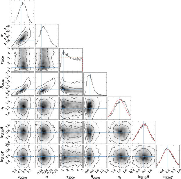
In Figure 2, we show the projected density profile $y_{\Delta}(x)=\Sigma(r_{\Delta}x)/\Sigma(r_{\Delta})$ of the individual CLASH clusters (gray lines), as well as the best-fit DK14 (blue), NFW (dashed black), and Einasto (solid black) fits. The results are shown for two different choices of the pivot overdensity, namely 200m (left panel) and 2500c (right panel). In the upper panels of Figure 3, we show the corresponding three-dimensional logarithmic slope $d\ln{\Delta\rho(r)/d\ln{r}}$ of the DK14 fit with $1\sigma$ errors (shaded area), as well as the NFW and Einasto slopes. Similarly, the lower panels show the logarithmic slope $d\ln\Sigma(R)/d\ln{R}$ of the best-fit surface mass density profiles. Finally, Figure 4 shows the one- and two-dimensional marginalized posterior distributions for the complete set of scaled DK14 parameters with $\Delta=\mathrm{200m}$, $\mbox{\boldmath$p$}=\{c_{\mathrm{200m}},\alpha,\tau_{\mathrm{200m}},B_{\mathrm{200m}},s_{\mathrm{e}},\beta,\gamma\}$. For all parameters, the global best-fit values coincide well with their respective peak values of the one-dimensional marginalized posterior distributions.

In the following sections, we discuss the fit quality as well as the inferred parameters for the inner ($r\lower 2.15277pt\hbox{$\;\buildrel<\over{\sim}\;$}r_{\mathrm{vir}}$) and outer regions of the profile.

3.1. Fit Quality

The ensemble mass profile in projection is remarkably well described by an NFW or Einasto profile out to $R\sim 1.2r_{\mathrm{200m}}$ or $R\sim 4.5r_{\mathrm{2500c}}$ (Figures 2 and 3), beyond which the data exhibit a flattening that is not modeled by those fitting functions. Note that to calculate $r_{\Delta}$ and $\Sigma(r_{\Delta})$ for each individual cluster (Section 2.1), we employed the spherical NFW fits of U16 obtained with a restricted fitting range of $R\leq 2h^{-1}\,\mathrm{Mpc}\sim r_{\mathrm{200m}}$. The results shown here thus ensure the self-consistency of our analysis.

As the outer profiles are expected to be most universal with respect to $\Delta=\mathrm{200m}$ (DK14), that definition is of particular relevance for the splashback radius. We thus use the DK14 model with $\Delta=\mathrm{200m}$ as a baseline model. This model has the best-fit $\chi^{2}$ of 180 for 232 degrees of freedom, corresponding to a probability of 99.5% to exceed the observed $\chi^{2}$ value, assuming the standard $\chi^{2}$ probability distribution function. The model is therefore in good agreement with the data. However, as we will discuss in Section 4.2, the improvement in the fit is not significant compared to the NFW or Einasto fit, implying that the parameters that describe the transition region and outer terms are not well constrained by the data. This is not surprising, because Figure 2 shows that the CLASH lensing data do not resolve the profile curvature in the transition region particularly well. Hence, the shape of the gradient feature at $r\sim r_{\mathrm{200m}}$, which locally deviates from the three-dimensional NFW and Einasto profiles (Figure 3), is specific to the assumed DK14 profile form.

We note that the $\chi^{2}$ values in Table 2 decrease with increasing overdensity $\Delta$, independent of the fitting function. The reason for this trend is that the inner $\Sigma$ profiles are more tightly constrained by the data, especially from the HST lensing analysis, so that scaling the $\Sigma$ profiles to higher overdensities reduces the overall scatter, which is dominated by the inner regions. We also note that the reduced $\chi^{2}$ values in Table 2 are systematically smaller than unity, which may indicate that the number of degrees of freedom is overestimated owing to the effects of nonlinear modeling (Andrae et al., 2010) and/or that the errors are conservatively overestimated. Since U16 found the reduced $\chi^{2}$ for their fits to the same input data to be $\lower 2.15277pt\hbox{$\;\buildrel>\over{\sim}\;$}1$ (their Table 4), it is unlikely that the errors are significantly overestimated.

3.2. The Inner Mass Profile: Shape and Self-similarity

The best-fit values of concentration shown in Table 2 agree well between the different fitting models. This similarity is also apparent in Figures 2 and 3, as the models have very similar shapes for both scaling overdensities shown. Furthermore, the best-fit values for the shape parameter $\alpha$ agree between the Einasto and DK14 fits, and lie in the range $0.18\lower 2.15277pt\hbox{$\;\buildrel<\over{\sim}\;$}\alpha\lower 2.15277pt\hbox{$\;\buildrel<\over{\sim}\;$}0.22$ with a typical $1\sigma$ uncertainty of $0.06$ for the DK14 model, and $0.17\lower 2.15277pt\hbox{$\;\buildrel<\over{\sim}\;$}\alpha\lower 2.15277pt\hbox{$\;\buildrel<\over{\sim}\;$}0.21$ for the Einasto model. An Einasto density profile with $\alpha\sim 0.2$ closely resembles an NFW profile (e.g., Ludlow et al., 2013).

The uncertainties on $c$ and $\alpha$ allow us to assess the impact of the scaling overdensity. If the profiles are most universal as a function of a particular radius definition, we expect the fractional uncertainty on the fit to be smallest in that definition. DK14 investigated the universality of halo density profiles, and found that the inner profiles are most universal in units of $r_{\mathrm{200c}}$. However, this statement refers primarily to the redshift scaling of different definitions, which we cannot test here owing to the limited redshift range of the CLASH sample. At fixed redshift and fixed mass, we expect any overdensity within a range around $r_{\mathrm{200c}}$ to lead to reasonably universal inner profiles, whereas for very extreme definitions the scatter in the profiles might increase.

These expectations are borne out in our results. The fractional uncertainties on NFW-$c$ and Einasto-$\alpha$ (the primary parameter that determines the shape of the profile for each model) are smallest for the 200m and virial scalings, and increase toward the highest overdensities (despite a lower $\chi^{2}$). However, the uncertainties on Einasto-$c$ are slightly lower at somewhat higher overdensities such as $\Delta=500$c. Overall, it appears that a rescaling with densities around $\Delta=\mathrm{200c}$ leads to relatively low uncertainties. Regardless of the profile model, scaling with $\Delta=2500$c results in significantly higher uncertainties. Since the determination of spherical overdensity radii (or masses) is not less certain at high overdensities (U16, their Section 4.2), we conclude that the increased uncertainty arises because the inner profiles are less universal at very high overdensities. Furthermore, we note that the relative insensitivity of the inner profiles to $\Delta$ is likely in part due to the sample selection based on X-ray regularity (Section 2.1), which is understood to significantly reduce the scatter in concentration (Meneghetti et al., 2014). The results have been confirmed by the CLASH full lensing analysis of U16 (see their Section 6.2, as well as Merten et al. 2015).

Most importantly, we find that scaling the profiles by any overdensity radius (except for $\Delta={\rm 2500c}$) improves the constraints on the best-fit parameters. As a result, the limits on concentration are tighter than those of U16 who scaled the profiles in physical units and found uncertainties of 8% on NFW-$c$, 11% on Einasto-$c$, and 18% on Einasto-$\alpha$ (see their Table 4).

$\begin{array}[]{c@{\hspace{.1in}}c}\includegraphics[scale={0.25},angle={0},clip]{Figs/f5a1.pdf}\hfil\hskip 7.22743pt&\includegraphics[scale={0.25},angle={0},clip]{Figs/f5b1.pdf}\\ \includegraphics[scale={0.25},angle={0},clip]{Figs/f5a2.pdf}\hfil\hskip 7.22743pt&\includegraphics[scale={0.25},angle={0},clip]{Figs/f5b2.pdf}\end{array}$

Figure 5.— Marginalized one-dimensional posterior probability distributions of the three-dimensional splashback radius (top panels) and mass (bottom panels) in scaled units, $R_{\mathrm{sp}}^{\mathrm{3D}}/r_{\Delta}$ and $M_{\mathrm{sp}}/M_{\Delta}$, for two different values of the chosen pivot overdensity, $\Delta=\mathrm{200m}$ (left panels) and $\mathrm{2500c}$ (right panels). The red vertical dashed lines indicate the 16th, 50th, and 84th percentiles of the distributions. The global best-fit model values of $R_{\mathrm{sp}}^{\mathrm{3D}}/r_{\Delta}$ and $M_{\mathrm{sp}}/M_{\Delta}$ are marked by a black vertical solid lines. The scales on the top axes denote $R_{\mathrm{sp}}^{\mathrm{3D}}$ and $M_{\mathrm{sp}}$ in physical units, converted using the effective overdensity radius $r_{\Delta}$ and mass $M_{\Delta}$ of the sample.

3.3. The Outer Profile and Splashback Radius

We now turn toward the outer profiles and particularly the inferred gradient profiles shown in Figure 3. A comparison of the three- and two-dimensional slopes highlights why detecting the splashback radius in surface density profiles is challenging in practice: even though there is a noticeable steepening in the three-dimensional slope, the two-dimensional slope drops very little, owing to projection effects (see Section 4.4).

Nevertheless, we can derive a splashback radius and mass from each of the MCMC samples of the DK14 parameters shown in Figure 4 (Equations A6 and A7). In Figure 5, we show the corresponding one-dimensional marginalized posterior distributions for $R_{\mathrm{sp}}^{\mathrm{3D}}$ and $M_{\mathrm{sp}}\equiv M(<R_{\mathrm{sp}}^{\mathrm{3D}})$, both in scaled units. The results are shown for two different values of the chosen pivot overdensity, $\Delta=\mathrm{200m}$ (left panels) and 2500c (right panels). In each panel, the vertical dashed lines indicate the 16th, 50th, and 84th percentiles of the marginalized posterior distribution. The locations of $R_{\mathrm{sp}}^{\mathrm{3D}}/r_{\Delta}$ and $M_{\mathrm{sp}}/M_{\Delta}$ derived from the best-fit model (Table 2) are indicated by vertical solid lines in Figure 5, and are in close agreement with the respective median values of the distributions. The posterior distributions show a tail extending toward large positive values of $R_{\mathrm{sp}}^{\mathrm{3D}}/r_{\Delta}$ and $M_{\mathrm{sp}}/M_{\Delta}$, associated with large values of the truncation parameter, $\tau_{\Delta}=r_{\mathrm{t}}/r_{\Delta}$ (Figure 4). A large $\tau_{\Delta}$ indicates a profile without a well-defined steepening feature. We thus place uninformative upper bounds on $R_{\mathrm{sp}}^{\mathrm{3D}}/r_{\Delta}$ and $M_{\mathrm{sp}}/M_{\Delta}$. On the other hand, we obtain tighter lower bounds on these parameters because the inner $\Sigma$ profiles of the clusters are well constrained by the combination of strong-lensing, weak-lensing shear and magnification data (U16).

Table 3 Constraints on the Splashback Radius and Mass

$\Delta$	$R_{\mathrm{sp}}^{\mathrm{3D}}/r_{\Delta}$	$R_{\mathrm{sp}}^{\mathrm{3D}}$	$M_{\mathrm{sp}}/M_{\Delta}$	$M_{\mathrm{sp}}$
		$(\mathrm{Mpc}/h)$		$(10^{15}M_{\odot}/h)$
200m	$>0.89$ ($1.23$)	$>1.83$ ($2.52$)	$>0.93$ ($1.13$)	$>1.21$ ($1.48$)
virial	$>0.91$ ($1.52$)	$>1.67$ ($2.78$)	$>0.94$ ($1.30$)	$>1.13$ ($1.56$)
200c	$>1.04$ ($1.90$)	$>1.52$ ($2.79$)	$>1.03$ ($1.55$)	$>1.04$ ($1.57$)
500c	$>1.37$ ($3.09$)	$>1.30$ ($2.94$)	$>1.31$ ($2.39$)	$>0.90$ ($1.64$)
2500c	$>2.69$ ($4.96$)	$>1.09$ ($2.00$)	$>2.91$ ($5.22$)	$>0.77$ ($1.38$)

Note. — Lower limits (68% CL) and best-fit model values (in parentheses) for the three-dimensional splashback radius and mass. The splashback radius and mass in physical length units were converted using the effective overdensity radius $r_{\Delta}^{\mathrm{eff}}$ and mass $M_{\Delta}^{\mathrm{eff}}$ of the sample, respectively.

Table 3 summarizes the 68% confidence lower limits and best-fit model values (in parentheses) on the splashback radius and mass. We also list $R_{\mathrm{sp}}^{\mathrm{3D}}$ and $M_{\mathrm{sp}}$ in physical length units converted with the effective overdensity radius ($r_{\Delta}^{\mathrm{eff}}$) and mass ($M_{\Delta}^{\mathrm{eff}}$) of the sample (Section 2.1). Using the fiducial scaling overdensity of $\Delta=\mathrm{200m}$, these lower limits are $R_{\mathrm{sp}}^{\mathrm{3D}}/r_{\mathrm{200m}}>0.89$ and $M_{\mathrm{sp}}/M_{\mathrm{200m}}>0.93$, corresponding to $R_{\mathrm{sp}}^{\mathrm{3D}}>1.83h^{-1}\,\mathrm{Mpc}$ and $M_{\mathrm{sp}}>1.21\times 10^{15}h^{-1}\,M_{\odot}$. We note that the location of the steepest slope in projection, $R_{\mathrm{sp}}^{\mathrm{2D}}/r_{\Delta}$, is smaller than $R_{\mathrm{sp}}^{\mathrm{3D}}/r_{\Delta}$ (Figure 3) because of projection effects (More et al., 2016). Using our best-fit base DK14 model ($\Delta=\mathrm{200m}$ in Table 2), we find $R_{\mathrm{sp}}^{\mathrm{2D}}/R_{\mathrm{sp}}^{\mathrm{3D}}\simeq 0.8$. We discuss the difference between the two- and three-dimensional splashback radii further in Section 4.4.

From a comparison of the lower bounds on the splashback radius and mass in Table 3, we see that the steepening feature is most pronounced when the cluster profiles are scaled by $r_{\mathrm{200m}}$, and is smeared out when scaled to higher overdensities, resulting in less strict lower limits (see also the right panels of Figure 3). This trend is consistent with the prediction of DK14 that halos reveal self-similar behavior in their outskirts when their profiles are expressed in units of spherical overdensity radii defined with respect to the mean density of the universe, especially $r_{\mathrm{200m}}$.

4. Discussion

In this section, we compare our results for the shape of the profile, concentration, and splashback radius with predictions from $N$-body simulations. We discuss observational and simulation effects that could potentially complicate our analysis.

4.1. The Impact of Priors

We imposed a number of priors on the parameters of the DK14 profile, namely on the slopes $\beta$ and $\gamma$, on the steepening radius $\tau_{\Delta}$, and on the outer profile slope $s_{\mathrm{e}}$ (see Figure 4). These priors were based on the results of DK14 for the median profiles of halo samples spanning a wide range of masses and mass accretion rates, and chosen conservatively, i.e. allowing a much larger range of parameter values than found for high-mass cluster halos in DK14. We find that imposing constraining theoretical priors leads to an inflated sensitivity to the splashback feature. As stated in Section 2.3, we use the DK14 profile as a flexible fitting function to determine the location of the steepest slope, $R_{\mathrm{sp}}^{\mathrm{3D}}$, which is an observable quantity. In this context, $\mbox{\boldmath$p$}=\{c_{\Delta},\alpha,\tau_{\Delta},B_{\Delta},s_{\mathrm{e}},\beta,\gamma\}$ are considered to be merely fitting parameters, and we allow them to take on values not expected from simulations, such as very large $\alpha$.

Nevertheless, one might worry that our inferences regarding $R_{\mathrm{sp}}^{\mathrm{3D}}$ are informed by the priors because they clearly inform the posterior of some parameters (Figure 4). In particular, the asymptotic slope of the 1-halo term, $\gamma$, is essentially unconstrained by the fit and relatively steep due to the prior (for example, $\gamma=0$ is effectively excluded). However, it is important to note that $\gamma$ (as well as $\beta$) has no impact on the DK14 profile if $\tau_{\Delta}$ is large, because the steepening then moves out of the observed region of the profile. Thus, the most critical prior is that on $\tau_{\Delta}$.

Our prior allows values of $\tau_{\Delta}$ up to 5, placing the steepening at $r_{\mathrm{t}}\lower 2.15277pt\hbox{$\;\buildrel<\over{\sim}\;$}10h^{-1}\,\mathrm{Mpc}$ which lies far outside the maximum radius of our data ($R\simeq 5h^{-1}\,\mathrm{Mpc}$). Thus, profiles with $\tau_{\mathrm{200m}}\lower 2.15277pt\hbox{$\;\buildrel>\over{\sim}\;$}2.5$ effectively reduce to an Einasto profile with a 2-halo term ($f_{\mathrm{trans}}\approx 1$) in the observed radial range. We have already demonstrated that a fit with these priors can reproduce a profile without steepening in the analysis of synthetic weak-lensing data (Figure 1). However, we note that, in combination with a higher value of $\alpha$ and a positive value of $B_{\Delta}$, even profiles with $\tau_{\mathrm{200m}}>2.5$ can reproduce a splashback feature in the observed radial range (with an inner profile steeper than the best-fit NFW/Einasto profile). We have confirmed that the resulting profiles are, in fact, a reasonable description of the data. Our priors also allow a profile with a negative 2-halo normalization, $B_{\Delta}\leq 0$ (i.e., underdense regions), which can produce a steepening gradient without an upturn feature. Here, the ensemble fits yield positive $\Delta\rho$ (i.e., $\rho>\rho_{\mathrm{m}}$) in the observed range because $\Sigma$ is constrained to be positive (U16).

In order to confirm that the $\tau_{\Delta}$ prior does not significantly affect our results, we have performed a fit with a flat prior of $\tau_{\mathrm{200m}}<20$, corresponding to $r_{\mathrm{t}}\lower 2.15277pt\hbox{$\;\buildrel<\over{\sim}\;$}40h^{-1}\,\mathrm{Mpc}$ for the CLASH sample. With this relaxed $\tau_{\Delta}$ prior, we find the same best-fit solution and a 68% CL lower bound of $R_{\mathrm{sp}}^{\mathrm{3D}}/r_{\mathrm{200m}}>0.90$, compared to $>0.89$ obtained with $\tau_{\mathrm{200m}}<5$. This difference represents a $1\%$ change, which is not significant given the current sensitivity. Moreover, we find no noticeable changes in the constraints on the density and gradient profiles shown in Figures 2 and 3. Therefore, we conclude that our results are sufficiently robust against the choice of the $\tau_{\Delta}$ prior.

4.2. Which Density Profile Does the CLASH Sample Prefer?

A robust outcome of our analysis is that, regardless of the pivot overdensity $\Delta$ chosen, the ensemble CLASH mass profile in projection is in full agreement with the NFW or Einasto profile out to $\sim r_{\mathrm{200m}}$, consistent with previous lensing results (e.g., Umetsu et al., 2011a, 2014, 2016; Newman et al., 2013; Okabe et al., 2013; Niikura et al., 2015; Okabe & Smith, 2016). This also ensures the self-consistency of our analysis, in which we used the NFW fits of U16 to calculate $r_{\Delta}$ and $\Sigma(r_{\Delta})$ for individual clusters, where the fitting range was restricted to $R\leq 2h^{-1}\,\mathrm{Mpc}\sim r_{\mathrm{200m}}$.

Our base DK14 model with $\Delta=\mathrm{200m}$ gives a slightly better fit than the corresponding NFW or Einasto model in terms of the best-fit $\chi^{2}$ values (Table 2). The relative improvements are $\Delta\chi^{2}=\chi^{2}_{\mathrm{NFW}}-\chi^{2}_{\mathrm{DK14}}\simeq 1$ and $\Delta\chi^{2}=\chi^{2}_{\mathrm{Einasto}}-\chi^{2}_{\mathrm{DK14}}\simeq 1$ for three and two additional free parameters, respectively. Hence, the improvement is not statistically significant, implying that our inference of the outskirt feature depends on the choice of the fitting function and priors.

As discussed in Section 2.3 and by More et al. (2016), we would apply two requirements to claim a detection of the splashback radius with a DK14 model, namely (1) that the location of the steepest slope in three dimensions with respect to $r_{\Delta}$ can be identified at high significance and (2) that this steepening is greater than that expected from a DK14 model with $f_{\mathrm{trans}}=1$ (i.e., $\tau_{\Delta}\gg 1$, reducing to an Einasto profile). The second criterion is important to ensure that the steepening is actually associated with a density caustic rather than the transition to the 2-halo term.

Given these criteria, we do not find sufficient evidence for the existence of a splashback feature in the CLASH lensing data because the data do not have the sensitivity necessary to resolve the profile curvature in the transition region. This result is not surprising, as demonstrated in our simulated experiment (Section 2.5). On the other hand, assuming the DK14 profile form and generic priors calibrated with numerical simulations, we have placed lower limits on the splashback radius of the CLASH clusters (Table 3), if it exists. Since we cannot rule out models with $f_{\mathrm{trans}}=1$, it is possible that the observed gradient feature in the outskirts is a statistical fluctuation. In Section 2.5, we showed that our analysis pipeline produces unbiased results in terms of both $\Sigma$ profiles and ensemble DK14 fits, and does not create spurious gradient features. Hence, the inferred outskirt feature is unlikely to arise from systematic errors.

An additional source of uncertainties in our scaling analysis is the statistical errors on the NFW parameters of individual clusters, which propagate into uncertainties in their scaling radius $R_{\Delta}$ and scaling density $\Sigma(R_{\Delta})$. In this work, these scaling parameters of individual clusters are fixed to their best-fit values from the NFW fits of U16. Hence, although our scaling analysis has led to significant improvements in the constraints on the inner profiles relative to the conventional stacking (see Section 4.3), these errors are likely to have smeared out local features to some level (Niikura et al., 2015). The degree of smearing can be assessed by marginalizing over uncertainties in the NFW parameters for all clusters, and such effects need to be accounted for in future studies with a larger statistical sample of clusters and with a higher statistical sensitivity.

$\begin{array}[]{c@{\hspace{.3in}}c}\includegraphics[scale={0.45},angle={0},clip]{Figs/f6a.pdf}\hfil\hskip 21.68121pt&\includegraphics[scale={0.45},angle={0},clip]{Figs/f6b.pdf}\end{array}$

Figure 6.— Comparison of our CLASH lensing constraints on $R_{\mathrm{sp}}^{\mathrm{3D}}/r_{\mathrm{200m}}$ against $\Lambda$CDM predictions at $z=0.337$ (gray lines, More et al., 2015). Left panel: the relation between mass accretion rate and splashback radius. The blue horizontal line and the shaded area represent, respectively, the best-fit model value and the 68% confidence interval of the DK14 parameter $R_{\mathrm{sp}}^{\mathrm{3D}}/r_{\mathrm{200m}}$ inferred for the CLASH sample (Figure 5). The CLASH lensing constraints on the splashback radius overlap with a broad representative range of mass accretion rates predicted for DM halos. Right panel: the relation between peak height and splashback radius. Similarly, the CLASH results (blue square with error bars) are in agreement with the theoretical expectation $R_{\mathrm{sp}}^{\mathrm{3D}}/r_{\mathrm{200m}}\simeq 0.97$ evaluated at the effective peak height of the CLASH sample, $\nu_{\mathrm{200m}}=4.0\pm 0.1$. The blue vertical dashed lines mark the range of $\nu_{\mathrm{200m}}$ peak heights covered by our sample. The observational results of More et al. (2016) for their full sample at $z=0.24$ are shown as a filled circle (see Section 4.5). Owing to the CLASH X-ray selection, there could be a bias toward higher values of $R_{\mathrm{sp}}^{\mathrm{3D}}/r_{\mathrm{200m}}$ for our sample.

4.3. Comparison with Simulation Results

We begin by making sure that our results for the standard profile parameters, namely the concentration and Einasto shape parameters, are congruent with expectations from simulations. The best-fit values for concentration are relatively independent of the fitting function chosen (Table 2): the NFW fit results in $c_{\mathrm{200c}}=3.66$, the Einasto fit in $c_{\mathrm{200c}}=3.30$, and the DK14 fit in $c_{\mathrm{200c}}=3.58$. These values are in excellent agreement with the model of Diemer & Kravtsov (2015) which estimates the mean concentration to be $c_{\mathrm{200c}}=3.65$ for $M_{\mathrm{200c}}=10.11\times 10^{14}h^{-1}\,M_{\odot}$, $z=0.337$, and the cosmology assumed in this paper. The model of Diemer & Kravtsov (2015) is based on NFW concentrations, whereas Einasto concentrations are expected to be about 10% lower at those masses and redshifts, in excellent agreement with our results (Figure 5 of Dutton & Macciò 2014, Meneghetti et al., 2014; Sereno et al., 2016). Our NFW constraints on the halo concentration $c_{\mathrm{200c}}=3.66\pm 0.11$ (with 16 clusters) are also in agreement with the expectations for the CLASH sample, namely a mean value of 3.87 and a standard deviation of 0.61, accounting for both selection and projection effects (Meneghetti et al., 2014).

Since the DK14 profile assumes an Einasto profile for the 1-halo term, the Einasto parameters are of particular interest. The Einasto profile varies in steepness with halo radius, at a rate given by a shape parameter $\alpha$. Gao et al. (2008) showed that this parameter is, to a good approximation, a function of only the peak height, $\nu$ (see also Dutton & Macciò, 2014). The CLASH mass corresponds to a peak height of $\nu_{\rm 200c}=3.76$ and thus $\alpha=0.29$, significantly higher than the values of about $0.2$ found in our fits. While the results of neither Gao et al. (2008) nor Dutton & Macciò (2014) are well constrained at such extreme peak heights, it is clear that $\alpha$ in their simulations exceeds $0.2$ significantly at high $\nu$. This tension already emerged as a $\approx 1\sigma$ difference in the analysis of U16. With the improved radial rescaling applied in this paper, the significance of the difference increases to $3.5\sigma$.

We have tested whether the steepening due to the splashback radius can bias the fitted $\alpha$ high compared to the value preferred by the inner profile. We find that such a bias can indeed appear depending on the fitted radial range (a larger range leads to larger bias) and the weights given to each radial bin. However, Dutton & Macciò (2014) fitted out to $1.2r_{\mathrm{vir}}$ and weighted the bins by the number of particles, and for these parameters the bias is smaller than $1\%$. Another possible explanation is that the X-ray-selected CLASH clusters are preferentially relaxed systems compared to the average population (Meneghetti et al., 2014). However, the relation of Gao et al. (2008) and Dutton & Macciò (2014) for $\alpha$ is based on halo samples that exclude unrelaxed halos, although this selection may not capture the entire effect present in the CLASH sample. On the other hand, taking into account baryonic effects in nonradiative hydrodynamical $N$-body simulations, Meneghetti et al. (2014) find that the Einasto shape parameter for cluster-size halos lies in the range $\alpha=0.21\pm 0.07$, indicating that our measurement is only moderately in tension with simulations.

Finally, we compare our inferences regarding the splashback radius $R_{\mathrm{sp}}^{\mathrm{3D}}$ with the simulation results of More et al. (2015) who predicted that the ratio of $R_{\mathrm{sp}}^{\mathrm{3D}}$ and $r_{\mathrm{200m}}$ depends primarily on the mass accretion rate of halos, with a less important dependence on redshift. In the left panel of Figure 6, we compare the ratio $R_{\mathrm{sp}}^{\mathrm{3D}}/r_{\mathrm{200m}}=1.23^{+2.33}_{-0.34}$ (blue shaded band), inferred for our sample at $z_{\mathrm{l}}^{\mathrm{eff}}=0.337$, with the mean relation in simulations (gray band),

$$\frac{R_{\mathrm{sp}}^{\mathrm{3D}}}{r_{\mathrm{200m}}}=0.58\left[1+0.63\Omega_{\mathrm{m}}(z)\right]\left(1+1.08\exp\left[-\frac{\Gamma}{2.26}\right]\right),$$ (9)

where $\Gamma\equiv d\ln{M_{\mathrm{vir}}}/d\ln{a}$ is the mass accretion rate (More et al., 2015). This comparison shows that the CLASH lensing constraints on the splashback radius overlap with a broad range of mass accretion rates $\Gamma$. Our lower $1\sigma$ (16th percentile) limit of $R_{\mathrm{sp}}^{\mathrm{3D}}/r_{\mathrm{200m}}\lower 2.15277pt\hbox{$\;\buildrel>\over{\sim}\;$}0.89$ translates into an upper limit on the accretion rate of $\Gamma\lower 2.15277pt\hbox{$\;\buildrel<\over{\sim}\;$}4.0$. This limit is not particularly informative, since only a very small fraction of halos experience such rapid accretion (DK14).

Since we cannot directly measure the mass accretion rate of the CLASH cluster sample, we cannot independently verify whether this prediction is congruent with observations. For this reason, More et al. (2015) also provide an approximate relation for the mean splashback radius as a function of peak height and redshift,

$$\frac{R_{\mathrm{sp}}^{\mathrm{3D}}}{r_{\mathrm{200m}}}=0.81\left(1+0.97\exp\left[-\frac{\nu_{\mathrm{200m}}}{2.44}\right]\right)\,.$$ (10)

The right panel of Figure 6 shows a comparison of this fitting function with our results for the splashback radius and the peak height of the CLASH cluster sample. Our inferred range of possible splashback radii covers the entire range of values suggested by the simulation results, showing that our results are generally compatible with simulations. While the results of More et al. (2015) were based on DM-only simulations, Lau et al. (2015) broadly confirmed the results of DK14 in hydrodynamical simulations of individual clusters. Thus, we have currently no reason to assume that baryons affect the location of the splashback radius significantly.

4.4. Projection Effects in Halo Profiles

In the previous sections, we defined $R_{\mathrm{sp}}^{\mathrm{3D}}$ as the halo radius where the logarithmic slope of the three-dimensional density profile is steepest. However, the quantity actually measured is the two-dimensional density profile, both when observing cluster member density profiles as in More et al. (2016) or the lensing signal of clusters as in this work. Thus, it is important to understand the relation between the location of the radii of the steepest slope in thee dimensions and in projection, $R_{\mathrm{sp}}^{\mathrm{3D}}$ and $R_{\mathrm{sp}}^{\mathrm{2D}}$.

We have investigated this relation using the simulated halo sample of More et al. (2015). In all cases, the steepening of the two-dimensional mass profile is less pronounced than that of the three-dimensional profile, as highlighted in Figure 14 of DK14. At high mass accretion rates ($\Gamma\geq 3$), $R_{\mathrm{sp}}^{\mathrm{2D}}/R_{\mathrm{sp}}^{\mathrm{3D}}$ approaches a fixed ratio of about $0.8$, in agreement with our measurements (Section 3.3). At lower mass accretion rates, however, the $R_{\mathrm{sp}}^{\mathrm{2D}}$ derived from the profiles exhibits huge scatter and a seemingly random pattern.

The difficulty in deriving a valid $R_{\mathrm{sp}}^{\mathrm{2D}}$ from projected measurements can be understood by considering a few realizations of the DK14 profile with a power-law outer profile representing the 2-halo term (see DK14 for details). The location of the steepest slope in three dimensions is a trade-off between the steepening 1-halo term and the 2-halo term. The steepening is less pronounced for halos with lower mass accretion rates. Thus, in projection, the 2-halo term has a substantial impact on the apparent location of $R_{\mathrm{sp}}^{\mathrm{2D}}$, which emerges at a much smaller radius that is unrelated to the steepening term (Figure 3), a problem that becomes more serious at small peak heights.

These results highlight the importance of forward-modeling the effects of the steepening based on the underlying three-dimensional density profile, rather than attempting to derive $R_{\mathrm{sp}}^{\mathrm{3D}}$ from $R_{\mathrm{sp}}^{\mathrm{2D}}$ directly (e.g., using Gaussian process modeling).

4.5. Compatibility with Measurements from Cluster Member Density Profiles

The splashback radius was first unambiguously detected in observations by More et al. (2016) who stacked surface number density profiles of cluster member galaxies for a large number of clusters. Their clusters were split into two subsamples with high and low concentrations of member galaxies ($c_{\mathrm{gal}}$) at fixed richness and redshift (Miyatake et al., 2016). These high- and low-$c_{\mathrm{gal}}$ samples were expected to represent populations of high and low $\Gamma$, respectively. However, Zu et al. (2016) have shown that the parameter $c_{\mathrm{gal}}$ used in More et al. (2016) is strongly contaminated by projection effects and is likely sensitive to the large-scale environment of the clusters rather than their internal structure. We thus limit our comparison to the full sample of More et al. (2016) whose inferred splashback radius is $R_{\mathrm{sp}}^{\mathrm{3D}}/r_{\mathrm{200m}}=0.837\pm 0.031$, with a weak-lensing mass of $M_{\mathrm{200m}}\simeq 1.87\times 10^{14}h^{-1}\,M_{\odot}$ at $z=0.24$ (S. More 2016, private communication).

Figure 6 shows that our lower limit on $R_{\mathrm{sp}}^{\mathrm{3D}}$ is higher than this value, but overlaps with the full-sample measurement at the $\sim 1\sigma$ level. We note that we expect the average mass accretion rate of the CLASH sample to be low due to a high fraction of relaxed objects (Meneghetti et al., 2014). Hence, owing to the selection effects, there could be a bias toward higher values of $R_{\mathrm{sp}}^{\mathrm{3D}}/r_{\mathrm{200m}}$ in our sample.

5. Summary

We have developed methods for modeling averaged cluster lensing profiles scaled to a chosen halo overdensity $\Delta$, which can be optimized for the extraction of features that are local in radius, in particular the steepening due to the splashback radius in the outskirts of collisionless DM halos. We have examined the ensemble mass distribution of 16 CLASH X-ray-selected clusters by forward-modeling the gravitational lensing data obtained by Umetsu et al. (2016). Our main conclusions are as follows.

• Regardless of the overdensity chosen, the CLASH ensemble mass profile in projection is remarkably well described by a scaled NFW or Einasto density profile out to $R\sim 1.2r_{\mathrm{200m}}\sim 2.5h^{-1}\,\mathrm{Mpc}$, beyond which the data exhibit a flattening with respect to the NFW or Einasto profile.

• We constrain the NFW halo concentration to $c_{\mathrm{200c}}=3.66\pm 0.11$ at $M_{\mathrm{200c}}\simeq 1.0\times 10^{15}h^{-1}\,M_{\odot}$, consistent with previous work based on the same input data (Umetsu et al., 2016). Our new analysis using scaled profiles provides tighter constraints on the halo shape and structural parameters ($c$ and $\alpha$) than the conventional stacking.

• We do not find statistically significant evidence for the existence of the splashback radius in the CLASH lensing data. At the current sensitivity, this result is in line with expectations from simulated, synthetic observations. Assuming the DK14 profile form and generic priors calibrated with simulations, we have placed a lower limit on the splashback radius of the clusters, if it exists, of $R_{\mathrm{sp}}^{\mathrm{3D}}/r_{\mathrm{200m}}>0.89$ or $R_{\mathrm{sp}}^{\mathrm{3D}}>1.83h^{-1}\,\mathrm{Mpc}$ at 68% confidence. This constraint is in agreement with $\Lambda$CDM predictions.

• The gradient feature in the outskirts is most pronounced for a scaling with $r_{\mathrm{200m}}$, consistent with simulation results of Diemer & Kravtsov (2014) and Lau et al. (2015).

The results obtained here are generally favorable in terms of the standard explanation for DM as effectively collisionless and nonrelativistic on sub-megaparsec scales and beyond, with an excellent match between lensing data and $\Lambda$CDM predictions for high-mass clusters. This study represents a first step toward using cluster gravitational lensing to examine detailed predictions from collisionless $\Lambda$CDM simulations regarding the shape and universality of the outer density profiles. Such predictions can, in principle, be unambiguously tested across a wide range of halo masses, redshifts, and accretion rates, with large statistical samples of clusters from ongoing and planned lensing surveys such as the Subaru Hyper Suprime-Cam survey (Miyazaki et al., 2015), the Dark Energy Survey, and the WFIRST and Euclid missions.

Appendix A Scaled DK14 Model

We express the scaled DK14 density profile as

$$f_{\Delta}(x)=f_{\mathrm{inner}}(x)\,f_{\mathrm{trans}}(x)+f_{\mathrm{outer}}(x)$$ (A1)

with

$$f_{\mathrm{inner}}(x) =\exp\left[-\frac{2}{\alpha}c_{\Delta}^{\alpha}(x^{\alpha}-1)\right],$$ (A2)

$$f_{\mathrm{trans}}(x) =\left[1+\left(\frac{x}{\tau_{\Delta}}\right)^{\beta}\right]^{-\frac{\gamma}{\beta}},$$

$$f_{\mathrm{outer}}(x) =\frac{B_{\Delta}}{\epsilon_{\Delta}+x^{s_{\mathrm{e}}}},$$

where $c_{\Delta}=r_{\Delta}/r_{\mathrm{s}}$, $\tau_{\Delta}=r_{\mathrm{t}}/r_{\Delta}$, $B_{\Delta}=b_{\mathrm{e}}(\rho_{\mathrm{m}}/\rho_{\Delta})(5r_{\mathrm{200m}}/r_{\Delta})^{s_{\mathrm{e}}}$ with $\rho_{\Delta}\equiv\rho_{\mathrm{Einasto}}(r_{\Delta})=\rho_{\mathrm{s}}\exp\left[-(2/\alpha)(c_{\Delta}^{\alpha}-1)\right]$, and $\epsilon_{\Delta}=\Delta_{\mathrm{max}}^{-1}(5r_{\mathrm{200m}}/r_{\Delta})^{s_{\mathrm{e}}}$. The (unscaled) DK14 density profile is obtained as $\Delta\rho(r)=\rho_{\Delta}f_{\Delta}(r/r_{\Delta})$. The derivatives of the inner, transition, and outer terms are

$$-xdf_{\mathrm{inner}}/dx =2c_{\Delta}^{\alpha}x^{\alpha}f_{\mathrm{inner}},$$ (A3)

$$-xdf_{\mathrm{trans}}/dx =\gamma\frac{(x/\tau_{\Delta})^{\beta}}{1+(x/\tau_{\Delta})^{\beta}}f_{\mathrm{trans}},$$

$$-xdf_{\mathrm{outer}}/dx =s_{\mathrm{e}}\frac{x^{s_{\mathrm{e}}}}{\epsilon_{\Delta}+x^{s_{\mathrm{e}}}}f_{\mathrm{outer}}.$$

The logarithmic gradient of the DK14 density profile $\Delta\rho(r)$ with $r=r_{\Delta}x$ is thus given by

$$\frac{d\ln\Delta\rho}{d\ln{r}}=\frac{d\ln{f_{\Delta}}}{d\ln{x}} = \left(x\frac{df_{\mathrm{inner}}}{dx}f_{\mathrm{trans}}+xf_{\mathrm{inner}}\frac{df_{\mathrm{trans}}}{dx}+x\frac{df_{\mathrm{outer}}}{dx}\right)\Big{/}f_{\Delta}$$ (A4)

$$= -\left[2(c_{\Delta}x)^{\alpha}f_{\mathrm{inner}}f_{\mathrm{trans}}+\gamma\frac{(x/\tau_{\Delta})^{\beta}}{1+(x/\tau_{\Delta})^{\beta}}f_{\mathrm{inner}}f_{\mathrm{trans}}+s_{\mathrm{e}}\frac{x^{s_{\mathrm{e}}}}{\epsilon_{\Delta}+x^{s_{\mathrm{e}}}}f_{\mathrm{outer}}\right]\Big{/}f_{\Delta}.$$ (A5)

For the Einasto model ($f_{\mathrm{trans}}=1$, $f_{\mathrm{outer}}=0$), $d\ln{\Delta\rho}/d\ln{r}=-2(c_{\Delta}x)^{\alpha}=-2(r/r_{\mathrm{s}})^{\alpha}$.

In this work, the splashback radius $R_{\mathrm{sp}}^{\mathrm{3D}}$ is defined as the location of the steepest slope of the three-dimensional mass distribution $\Delta\rho(r)$. For a given set of the DK14 model parameters, we find the scaled splashback radius $x_{\mathrm{sp}}\equiv R_{\mathrm{sp}}^{\mathrm{3D}}/r_{\Delta}$ from

$$x_{\mathrm{sp}}=\mathop{\rm arg~{}min}\limits_{x}\frac{d\ln{f_{\Delta}}}{d\ln{x}}.$$ (A6)

The ratio of the splashback mass $M_{\mathrm{sp}}=M(<R_{\mathrm{sp}}^{\mathrm{3D}})$ to the overdensity mass $M_{\Delta}=M(<r_{\Delta})$ is given by

$$\frac{M_{\mathrm{sp}}^{\mathrm{3D}}}{M_{\Delta}}=\frac{\int_{0}^{x_{\mathrm{sp}}}\!dx\,x^{2}f_{\Delta}(x)}{\int_{0}^{1}\!dx\,x^{2}f_{\Delta}(x)}.$$ (A7)

Appendix B Synthetic Weak-lensing Data

We create a total of 50 source realizations of synthetic shear and magnification catalogs for our sample of 16 CLASH clusters, each of which is modeled as a spherical NFW halo specified by its redshift $z_{\mathrm{l}}$ (Table 1) and its parameters $M_{\mathrm{200c}}$ and $c_{\mathrm{200c}}$, which were fixed to the observed central values (Table 2 of U16).

For each NFW cluster, we consider two configurations of the outer density profile, one with and one without a splashback-like feature. For the latter, the total density profile is given by a single NFW profile, $\Delta\rho(r)=\rho_{\mathrm{NFW}}(r|M_{\mathrm{200c}},c_{\mathrm{200c}},z)$. For the former, we employ a composite lens model that produces an approximate splashback feature. We cannot use the DK14 profile directly because it is not implemented in the glafic software used to perform ray-tracing simulations as described below. However, the code does implement a steepening 1-halo term given by the truncated NFW profile of Baltz et al. (2009, BMO), $\rho_{\mathrm{BMO}}(r)$. We approximate the 2-halo term by a softened isothermal (SI) profile, $\rho_{\mathrm{SI}}(r)$: $\Delta\rho=\rho_{\mathrm{BMO}}+\rho_{\mathrm{SI}}$. The BMO density profile is expressed as $\rho_{\mathrm{BMO}}(r)=\rho_{\mathrm{NFW}}(r|M_{\mathrm{200c}},c_{\mathrm{200c}},z)\times f_{\mathrm{trans}}(r|\beta,\gamma,r_{\mathrm{t}})$ with $\beta=2$ and $\gamma=4$. The truncation radius $r_{\mathrm{t}}$ is set to $r_{\mathrm{t}}=1.1r_{\mathrm{vir}}\approx r_{\mathrm{200m}}$ We take the outer SI profile to be $\rho_{\mathrm{SI}}(r)=\rho_{\mathrm{c}}/[1+(r/r_{\mathrm{c}})^{2}]$ with $\rho_{\mathrm{c}}=1.5\times 10^{12}h^{2}\,M_{\odot}$ Mpc^-3 and $r_{\mathrm{c}}=2.2h^{-1}\,\mathrm{Mpc}$, so as to give a splashback feature at $R_{\mathrm{sp}}^{\mathrm{3D}}/r_{\mathrm{200m}}\sim 0.9$ for our CLASH sample. Here, the normalization of the SI profile is chosen to be three times lower than that of the 2-halo term in projection (Umetsu et al., 2014, see their Figure 7), because the standard halo model ($\Delta\rho=\rho_{\mathrm{BMO}}+\rho_{\mathrm{2h}}$), by design, does not produce a steepening relative to the NFW profile (Oguri & Hamana, 2011, see their Figure 2).

In general, source galaxy catalogs used for the shear and the magnification analysis are different because we apply different size, magnitude, and color cuts in source selection for measuring the shear and the magnification effects (Umetsu et al., 2014). We assume, for simplicity, that the two galaxy samples are identical. We ignore the cosmic noise contribution from projected uncorrelated large-scale structures here because it is subdominant in the total error budget (see Figure 1 of U16). For all clusters, we assume the same survey parameters and source properties as described below.

To produce synthetic magnification-bias data sets, we perform ray-tracing simulations with both NFW and BMO+SI lenses (Wright & Brainerd, 2000; Baltz et al., 2009; Oguri & Hamana, 2011) using the public package glafic (Oguri, 2010). We assume a maximally depleted sample of sources with $s\equiv d\log_{10}N(<m)/dm=0$, for which the effect of magnification bias is purely geometric and their lensed source counts can be inferred from the lensed image positions. We randomly distribute $N_{\mathrm{s}}=14,336$ source galaxies over an area of $32\times 32$ arcmin² in the source plane centered on the cluster. This corresponds to an unlensed source density of $\overline{n}_{\mathrm{s}}=14$ galaxies per arcmin², matched to the typical (median) value found in the CLASH weak-lensing observations of Umetsu et al. (2014, their Table 4). The source plane is placed at a redshift of $z_{\mathrm{s}}=1.0$, the median depth of their magnification samples (Umetsu et al., 2014).

For creation of synthetic shear catalogs, we draw $N_{\mathrm{s}}$ random source ellipticities from the Gaussian intrinsic ellipticity distribution given by Equation (12) of Schneider et al. (2000), with the rms intrinsic ellipticity assumed to be $0.3$. For each galaxy, we transform the source ellipticity into the image ellipticity at the image position according to Equation (1) of Schneider et al. (2000).

Our simulations include the following major steps of data analysis, signal reconstruction, and modeling processes:

1. Measurements of the reduced tangential shear and magnification bias profiles in $N_{\mathrm{WL}}=10$ log-spaced radial bins over the radial range $\theta\in[0.9\arcmin,16\arcmin]$ (Section 2.1) from the respective input source catalogs, following the analysis procedures described in Umetsu et al. (2014) and U16.

2. Reconstructions of the projected mass profile ($\Sigma$) from the binned shear and magnification constraints obtained in the first step.

3. Ensemble characterization of the cluster $\Sigma$ profiles using the scaled DK14 model and the priors described in Sections 2.3 and 2.4.

For the second step, we use the cluster lensing mass inversion (clumi) code (Umetsu et al., 2011b; Umetsu, 2013) as implemented in U16 but without using inner strong-lensing constraints, and assume perfect knowledge of the source properties, namely $z_{\mathrm{s}}=1.0$, $\overline{n}_{\mathrm{s}}=14$ galaxies arcmin^-2, and $s=0$. Otherwise, synthetic data are processed in the same manner as the CLASH data described in Section 2.1. In the third step, we find, for each source realization, the global maximum a posteriori estimate of the joint posterior distribution to infer the best-fit DK14 parameters.

References

- Adhikari et al. (2014) Adhikari, S., Dalal, N., & Chamberlain, R. T. 2014, J. Cosmology Astropart. Phys, 11, 019
- Adhikari et al. (2016) Adhikari, S., Dalal, N., & Clampitt, J. 2016, J. Cosmology Astropart. Phys, 7, 022
- Andrae et al. (2010) Andrae, R., Schulze-Hartung, T., & Melchior, P. 2010, ArXiv e-prints, arXiv:1012.3754 [astro-ph.IM]
- Applegate et al. (2014) Applegate, D. E., von der Linden, A., Kelly, P. L., et al. 2014, MNRAS, 439, 48
- Baltz et al. (2009) Baltz, E. A., Marshall, P., & Oguri, M. 2009, J. Cosmology Astropart. Phys, 1, 15
- Bartelmann & Schneider (2001) Bartelmann, M., & Schneider, P. 2001, Phys. Rep., 340, 291
- Becker & Kravtsov (2011) Becker, M. R., & Kravtsov, A. V. 2011, ApJ, 740, 25
- Beraldo e Silva et al. (2013) Beraldo e Silva, L. J., Lima, M., & Sodré, L. 2013, MNRAS, 436, 2616
- Bertschinger (1985) Bertschinger, E. 1985, ApJS, 58, 39
- Bhattacharya et al. (2013) Bhattacharya, S., Habib, S., Heitmann, K., & Vikhlinin, A. 2013, ApJ, 766, 32
- Broadhurst et al. (2005a) Broadhurst, T., Takada, M., Umetsu, K., et al. 2005a, ApJ, 619, L143
- Broadhurst et al. (2005b) Broadhurst, T., Benítez, N., Coe, D., et al. 2005b, ApJ, 621, 53
- Bullock et al. (2001) Bullock, J. S., Kolatt, T. S., Sigad, Y., et al. 2001, MNRAS, 321, 559
- Chiu et al. (2016) Chiu, I., Dietrich, J. P., Mohr, J., et al. 2016, MNRAS, 457, 3050
- Coe et al. (2010) Coe, D., Benítez, N., Broadhurst, T., & Moustakas, L. A. 2010, ApJ, 723, 1678
- Coe et al. (2012) Coe, D., Umetsu, K., Zitrin, A., et al. 2012, ApJ, 757, 22
- Coupon et al. (2013) Coupon, J., Broadhurst, T., & Umetsu, K. 2013, ApJ, 772, 65
- Cuesta et al. (2008) Cuesta, A. J., Prada, F., Klypin, A., & Moles, M. 2008, MNRAS, 389, 385
- Diego et al. (2015) Diego, J. M., Broadhurst, T., Benitez, N., et al. 2015, MNRAS, 446, 683
- Diemer (2015) Diemer, B. 2015, Colossus: COsmology, haLO, and large-Scale StrUcture toolS, Astrophysics Source Code Library, ascl:1501.016
- Diemer & Kravtsov (2014) Diemer, B., & Kravtsov, A. V. 2014, ApJ, 789, 1
- Diemer & Kravtsov (2015) —. 2015, ApJ, 799, 108
- Diemer et al. (2013) Diemer, B., More, S., & Kravtsov, A. V. 2013, ApJ, 766, 25
- Du & Fan (2014) Du, W., & Fan, Z. 2014, ApJ, 785, 57
- Du et al. (2015) Du, W., Fan, Z., Shan, H., et al. 2015, ApJ, 814, 120
- Dunkley et al. (2005) Dunkley, J., Bucher, M., Ferreira, P. G., Moodley, K., & Skordis, C. 2005, MNRAS, 356, 925
- Dutton & Macciò (2014) Dutton, A. A., & Macciò, A. V. 2014, MNRAS, 441, 3359
- Einasto (1965) Einasto, J. 1965, Trudy Astrofizicheskogo Instituta Alma-Ata, 5, 87
- Fillmore & Goldreich (1984) Fillmore, J. A., & Goldreich, P. 1984, ApJ, 281, 1
- Ford et al. (2014) Ford, J., Hildebrandt, H., Van Waerbeke, L., et al. 2014, MNRAS, 439, 3755
- Gao et al. (2008) Gao, L., Navarro, J. F., Cole, S., et al. 2008, MNRAS, 387, 536
- Gelman & Rubin (1992) Gelman, A., & Rubin, D. B. 1992, Statist. Sci., 7, 457
- Gruen et al. (2015) Gruen, D., Seitz, S., Becker, M. R., Friedrich, O., & Mana, A. 2015, MNRAS, 449, 4264
- Gruen et al. (2014) Gruen, D., Seitz, S., Brimioulle, F., et al. 2014, MNRAS, 442, 1507
- Gunn & Gott (1972) Gunn, J. E., & Gott, III, J. R. 1972, ApJ, 176, 1
- Hikage et al. (2013) Hikage, C., Mandelbaum, R., Takada, M., & Spergel, D. N. 2013, MNRAS, 435, 2345
- Hildebrandt et al. (2011) Hildebrandt, H., Muzzin, A., Erben, T., et al. 2011, ApJ, 733, L30
- Hjorth & Williams (2010) Hjorth, J., & Williams, L. L. R. 2010, ApJ, 722, 851
- Hoekstra (2003) Hoekstra, H. 2003, MNRAS, 339, 1155
- Hoekstra et al. (2015) Hoekstra, H., Herbonnet, R., Muzzin, A., et al. 2015, MNRAS, 449, 685
- Jauzac et al. (2014) Jauzac, M., Clément, B., Limousin, M., et al. 2014, MNRAS, 443, 1549
- Jimeno et al. (2015) Jimeno, P., Broadhurst, T., Coupon, J., Umetsu, K., & Lazkoz, R. 2015, MNRAS, 448, 1999
- Johnston et al. (2007) Johnston, D. E., Sheldon, E. S., Tasitsiomi, A., et al. 2007, ApJ, 656, 27
- Kitayama et al. (1998) Kitayama, T., Sasaki, S., & Suto, Y. 1998, PASJ, 50, 1
- Lau et al. (2015) Lau, E. T., Nagai, D., Avestruz, C., Nelson, K., & Vikhlinin, A. 2015, ApJ, 806, 68
- Ludlow et al. (2013) Ludlow, A. D., Navarro, J. F., Boylan-Kolchin, M., et al. 2013, MNRAS, 432, 1103
- Mansfield et al. (2016) Mansfield, P., Kravtsov, A. V., & Diemer, B. 2016, arXiv:1612.01531, arXiv:1612.01531
- Medezinski et al. (2013) Medezinski, E., Umetsu, K., Nonino, M., et al. 2013, ApJ, 777, 43
- Melchior et al. (2016) Melchior, P., Gruen, D., McClintock, T., et al. 2016, ArXiv e-prints, arXiv:1610.06890
- Meneghetti et al. (2014) Meneghetti, M., Rasia, E., Vega, J., et al. 2014, ApJ, 797, 34
- Merten et al. (2015) Merten, J., Meneghetti, M., Postman, M., et al. 2015, ApJ, 806, 4
- Miyatake et al. (2016) Miyatake, H., More, S., Takada, M., et al. 2016, Physical Review Letters, 116, 041301
- Miyazaki et al. (2015) Miyazaki, S., Oguri, M., Hamana, T., et al. 2015, ApJ, 807, 22
- More et al. (2015) More, S., Diemer, B., & Kravtsov, A. V. 2015, ApJ, 810, 36
- More et al. (2016) More, S., Miyatake, H., Takada, M., et al. 2016, ApJ, 825, 39
- Navarro et al. (1997) Navarro, J. F., Frenk, C. S., & White, S. D. M. 1997, ApJ, 490, 493
- Newman et al. (2013) Newman, A. B., Treu, T., Ellis, R. S., et al. 2013, ApJ, 765, 24
- Niikura et al. (2015) Niikura, H., Takada, M., Okabe, N., Martino, R., & Takahashi, R. 2015, PASJ, 67, 103
- Oguri (2010) Oguri, M. 2010, glafic: Software Package for Analyzing Gravitational Lensing, ascl:1010.012, astrophysics Source Code Library
- Oguri & Hamana (2011) Oguri, M., & Hamana, T. 2011, MNRAS, 414, 1851
- Oguri & Takada (2011) Oguri, M., & Takada, M. 2011, Phys. Rev. D, 83, 023008
- Okabe & Smith (2016) Okabe, N., & Smith, G. P. 2016, MNRAS, 461, 3794
- Okabe et al. (2013) Okabe, N., Smith, G. P., Umetsu, K., Takada, M., & Futamase, T. 2013, ApJ, 769, L35
- Okabe et al. (2010) Okabe, N., Takada, M., Umetsu, K., Futamase, T., & Smith, G. P. 2010, PASJ, 62, 811
- Patej & Loeb (2016) Patej, A., & Loeb, A. 2016, ApJ, 824, 69
- Penna-Lima et al. (2016) Penna-Lima, M., Bartlett, J. G., Rozo, E., et al. 2016, ArXiv e-prints, arXiv:1608.05356
- Planck Collaboration et al. (2014) Planck Collaboration, Ade, P. A. R., Aghanim, N., et al. 2014, A&A, 566, A54
- Postman et al. (2012) Postman, M., Coe, D., Benítez, N., et al. 2012, ApJS, 199, 25
- Rozo & Schmidt (2010) Rozo, E., & Schmidt, F. 2010, arXiv, 1009.5735, arXiv:1009.5735 [astro-ph.CO]
- Schive et al. (2014) Schive, H.-Y., Chiueh, T., & Broadhurst, T. 2014, Nature Physics, 10, 496
- Schneider et al. (2000) Schneider, P., King, L., & Erben, T. 2000, A&A, 353, 41
- Sereno et al. (2016) Sereno, M., Fedeli, C., & Moscardini, L. 2016, J. Cosmology Astropart. Phys, 1, 042
- Sereno et al. (2015) Sereno, M., Veropalumbo, A., Marulli, F., et al. 2015, MNRAS, 449, 4147
- Shi (2016) Shi, X. 2016, MNRAS, 459, 3711
- Spergel & Steinhardt (2000) Spergel, D. N., & Steinhardt, P. J. 2000, Physical Review Letters, 84, 3760
- Tully (2015) Tully, R. B. 2015, AJ, 149, 54
- Umetsu (2013) Umetsu, K. 2013, ApJ, 769, 13
- Umetsu & Broadhurst (2008) Umetsu, K., & Broadhurst, T. 2008, ApJ, 684, 177
- Umetsu et al. (2011a) Umetsu, K., Broadhurst, T., Zitrin, A., et al. 2011a, ApJ, 738, 41
- Umetsu et al. (2011b) Umetsu, K., Broadhurst, T., Zitrin, A., Medezinski, E., & Hsu, L. 2011b, ApJ, 729, 127
- Umetsu et al. (2016) Umetsu, K., Zitrin, A., Gruen, D., et al. 2016, ApJ, 821, 116
- Umetsu et al. (2012) Umetsu, K., Medezinski, E., Nonino, M., et al. 2012, ApJ, 755, 56
- Umetsu et al. (2014) —. 2014, ApJ, 795, 163
- Umetsu et al. (2015) Umetsu, K., Sereno, M., Medezinski, E., et al. 2015, ApJ, 806, 207
- von der Linden et al. (2014) von der Linden, A., Allen, M. T., Applegate, D. E., et al. 2014, MNRAS, 439, 2
- Wechsler et al. (2002) Wechsler, R. H., Bullock, J. S., Primack, J. R., Kravtsov, A. V., & Dekel, A. 2002, ApJ, 568, 52
- Williams & Hjorth (2010) Williams, L. L. R., & Hjorth, J. 2010, ApJ, 722, 856
- Wright & Brainerd (2000) Wright, C. O., & Brainerd, T. G. 2000, ApJ, 534, 34
- Zhao et al. (2009) Zhao, D. H., Jing, Y. P., Mo, H. J., & Börner, G. 2009, ApJ, 707, 354
- Ziparo et al. (2016) Ziparo, F., Smith, G. P., Okabe, N., et al. 2016, MNRAS, 463, 4004
- Zitrin et al. (2009) Zitrin, A., Broadhurst, T., Umetsu, K., et al. 2009, MNRAS, 396, 1985
- Zitrin et al. (2013) Zitrin, A., Meneghetti, M., Umetsu, K., et al. 2013, ApJ, 762, L30
- Zitrin et al. (2015) Zitrin, A., Fabris, A., Merten, J., et al. 2015, ApJ, 801, 44
- Zu et al. (2016) Zu, Y., Mandelbaum, R., Simet, M., Rozo, E., & Rykoff, E. S. 2016, ArXiv e-prints, arXiv:1611.00366