Dynamic Reductions for Model Checking Concurrent Software

Abstract

Symbolic model checking of parallel programs stands and falls with effective methods of dealing with the explosion of interleavings. We propose a dynamic reduction technique to avoid unnecessary interleavings. By extending Lipton’s original work with a notion of bisimilarity, we accommodate dynamic transactions, and thereby reduce dependence on the accuracy of static analysis, which is a severe bottleneck in other reduction techniques.

The combination of symbolic model checking and dynamic reduction techniques has proven to be challenging in the past. Our generic reduction theorem nonetheless enables us to derive an efficient symbolic encoding, which we implemented for IC3 and BMC. The experiments demonstrate the power of dynamic reduction on several case studies and a large set of SVCOMP benchmarks.

1 Introduction

The rise of multi-threaded software—a consequence of a necessary technological shift from ever higher frequencies to multi-core architectures—exacerbates the challenge of verifying programs automatically. While automated software verification has made impressive advances recently thanks to novel symbolic model checking techniques, such as lazy abstraction [26, 6], interpolation [33], and IC3 [9] for software [7, 10], multi-threaded programs still pose a formidable challenge.

The effectiveness of model checking in the presence of concurrency is severely limited by the state explosion caused through thread interleavings. Consequently, techniques that avoid thread interleavings, such as partial order reduction (POR) [38, 41, 19] or Lipton’s reduction [32], are crucial to the scalability of model checking, while also benefitting other verification approaches [18, 12, 15].

These reduction techniques, however, rely heavily on the identification of statements that are either independent or commute with the statements of all other threads, i.e. those that are globally independent. For instance, the single-action rule [31]—a primitive precursor of Lipton reduction—states that a sequential block of statements can be considered an atomic transaction if all but one of the statements are globally independent. Inside an atomic block, all interleavings of other threads can be discarded, thus yielding the reduction.

Identifying these globally independent statements requires non-local static analyses. In the presence of pointers, arrays, and complicated branching structures, however, the results of an up-front static analysis are typically extremely conservative, thus a severe bottleneck for good reduction.

fig:illustration shows an example with two threads (T1 and T2). Let’s assume static analysis can establish that pointers p and q never point to the same memory throughout the program’s (parallel) execution. This means that statements involving the pointers are globally independent, hence they globally commute, e.g. an interleaving *p++; *q = 1 always yields the same result as *q = 1; *p++;. Assuming that *p++; is also independent of the other statements from T2 (b = 2 and c = 3), we can reorder any trace of the parallel program to a trace where *p++ and *q = 2 occur subsequently without affecting the resulting state. The figure shows one example. Therefore, a syntactic transformation from *p++; *q = 2 to atomic{*p++; *q = 2} is a valid static reduction.

Ω1: *p++;Ω2: *q = 2;Ω\end{verbatim}Ω\end{minipage}Ω

 (T1)

Ω1: b = 2;Ω2: c = 3;Ω3: *q = 1;Ω\end{verbatim}Ω\end{minipage}Ω

 (T2)

Ω1: if (pc_T2 == 1){Ω2: *p++;Ω3: *q = 2;Ω} else { atomic{Ω4: *p++;Ω5: *q = 2; }}Ω\end{verbatim}Ω\end{minipage}Ω

 (T1’) Figure 1: (Left) C code for threads T1 and T2. (Middle) Reordering (dotted lines) a multi-threaded execution trace (T1’s actions are represented with straight arrows and T2’s with ‘dashed’ arrows). (Right) The instrumented code for T1.

Still, it is often hard to prove that pointers do not overlap throughout a program’s execution. Moreover, in many cases, pointers might temporarily overlap at some point in the execution. For instance, assume that initially p points to the variable b. This means that statements b = 2 and *p++ no longer commute, because b = 2; b++ yields a different result than b++; b = 2. Nevertheless, if b = 2 already happened, then we can still swap instructions and achieve the reduction as shown in fig:illustration. Traditional, static reduction methods cannot distinguish whether b = 2 already happened and yield no reduction. sec:motivation provides various other real-world examples of hard cases for static analysis.

In sec:instrument, we propose a dynamic reduction method that is still based on a similar syntactic transformation. Instead of merely making sequences of statements atomic, it introduces branches as shown in fig:illustration (T1’). A dynamic commutativity condition determines whether the branch with or without reduction is taken. In our example, the condition checks whether the program counter of T2 (pc_T2) still points to the statement b = 2 (pc_T2 == 1). In that case, no reduction is performed, otherwise the branch with reduction is taken. In addition to conditions on the program counters, we provide other heuristics comparing pointer and array values dynamically.

The instrumented code (T1’) however poses one problem: the branching condition no longer commutes with the statement that enables it. In this case, the execution of b = 2 disables the condition, thus before executing b = 2, T1’ ends up at Line 2, whereas after b = 2 it ends up at Line 4 (see fig:noncommutativity).

Figure 2: Loss of commutativity

Figure 3: Bisimulation (T1)

To remedy this, we require in sec:reduction that the instrumentation guarantees that the target states in both branches are bisimilar. fig:bisim-T1 shows that locations 2 and 4 of T1’ are bimilar, written $2\cong 4$, which implies that any statement executable from the one is also executable from the other ending again in a bisimilar location ($3\cong 5$). As bisimularity is preserved under parallel composition $(4,2)\cong(2,2)$, we can prove the correctness of our dynamic reduction method in app:proofs.

The benefit of our syntactic approach is that the technique can be combined with symbolic model checking checking techniques (sec:encoding provides an encoding for our lean instrumentation). Thus far, symbolic model checkers only supported more limited and static versions of reduction techniques as discussed in sec:related.

We implemented the dynamic reduction and encoding for LLVM bitcode, mainly to enable support for C/C++ programs without dealing with their intricate semantics (the increased instruction count of LLVM bitcode is mitigated by the reduction). The encoded transition relation is then passed to the Vienna Verification Tool (VVT) [24], which implements both BMC and IC3 algorithms extended with abstractions [7]. Experimental evaluation shows that (sec:experiments) dynamic reduction can yield several orders of magnitude gains in verification times.

2 Motivating Examples

int *data = NULL; void worker_thread(int tid) { c: if (data == NULL) { d: int *tmp = read_from_disk(1024); W: if (!CAS(&data, NULL, tmp)) free(tmp); } for (int i = 0; i < 512; i++) R: process(data[i + tid * 512]); } int main () { a: pthread_create(worker_thread, 0); // T1 b: pthread_create(worker_thread, 1); // T2 }

Figure 4: Lazy initialization

Lazy initialization

We illustrate our method with the code in fig:lazy. The main function starts two threads executing the worker_thread function, which processes the contents of data in the for loop at the end of the function. Using a common pattern, a worker thread lazily delays the initialization of the global data pointer until it is needed. It does this by reading some content from disc and setting the pointer atomically via a compare-and-swap operation (CAS) at label W (whose semantics here is an atomic C-statement: if (data==NULL) { data = tmp; return 1; } else return 0;). If it fails (returns 0), the locally allocated data is freed as the other thread has won the race.

The subsequent read access at label R is only reachable once data has been initialized. Consequently, the write access at W cannot possibly interfere with the read accesses at R, and the many interleavings caused by both threads executing the for loop can safely be ignored by the model checker. This typical pattern is however too complex for static analysis to efficiently identify, causing the model checker to conservatively assume conflicting accesses, preventing any reduction.

Ωint T[10] = {E,E,22,35,46,25,E,E,91,E};Ω\parint find-or-put(int v) {Ωint hash = v / 10;Ωfor (int i = 0; i < 10; i++) {Ωint index = (i + hash) if (CAS(&T[index], E, v)) {Ωreturn INSERTED;Ω} else if (T[index] == v)Ωreturn FOUND;Ω}Ωreturn TABLE_FULL;Ω}Ωint main() {Ωpthread_create(find-or-put, 25);Ωpthread_create(find-or-put, 42);Ωpthread_create(find-or-put, 78);Ω}Ω\end{verbatim}Ω\end{minipage}Ω

Ωint x = 0, y = 0;Ωint *p1, *p2;Ω\parvoid worker(int *p) {Ωwhile (*p < 1024)Ω*p++;Ω}Ωint main(){Ωa: if (*)Ωb: { p1 = &x; p2 = &y; }ΩelseΩc: { p1 = &y; p2 = &x; }Ωpthread_create(worker, p1); // T1Ωpthread_create(worker, p2); // T2Ωpthread_join(t1);Ωpthread_join(t2);Ωreturn x+y;Ω}Ω\end{verbatim}Ω\end{minipage}Ω

Figure 6: Load balancing.

Figure 5: Lockless hash table.

Hash table

The code in ex:ht implements a lockless hash table (from [30]) inserting a value v by scanning the bucket array T starting from hash, the hash value calculated from v. If an empty bucket is found (T[index]==E), then v is atomically inserted using the CAS operation. If the bucket is not empty, the operation checks whether the value was already inserted in the bucket (T[index] == v). If that is not the case, then it probes the next bucket of T until either v is found to be already in the table, or it is inserted in an empty slot, or the table is full. This basic bucket search order is called a linear probe sequence.

A thread performing find-or-put(25), for instance, merely reads buckets T[2] to T[5]. However, other threads might write an empty bucket, thus causing interference. To show that these reads are independent, the static analysis would have to demonstrate that the writes happen to different buckets. Normally this is done via alias analysis that tries to identify the buckets that are written to (by the CAS operation). However, because of the hashing and the probe sequence, such an analysis can only conclude that all buckets may be written. So all operations involving T will be classified as non-movers, also the reads. However if we look at the state of individual buckets, it turns out that a common pattern is followed using the CAS operation: a bucket is only written when it is empty, thereafter it doesn’t change. In other words, when a bucket T[i] does not contain E, then any operation on it is a read and consequently is independent.

Load balancing

ex:pointers shows a simplified example of a common pattern in multi-threaded software; load balancing: The work to be done (counting to 2048) is split up between two threads (each of which counts to 1024). The work assignment is represented by pointers p1 and p2, and a dynamic hand-off to one of the two threads is simulated using non-determinism (the first if branch). Static analysis cannot establish the fact that the partitions are independent, because they are assigned dynamically. But because the pointer is unmodified after assignment, its dereference commutes with that in other worker threads.

In sec:dynamic, we show how the discussed operations in all three examples can become dynamic movers, allowing for more reduction.

3 Preliminaries

A concurrent program consists of a finite number of sequential procedures, one for each thread $i$. We model the syntax of each thread $i$ by a control flow graph (CFG) $G_{i}=(V_{i},\delta_{i})$ with $\delta_{i}\subseteq V_{i}\times A\times V_{i}$ and $A$ being the set of actions, i.e., statements. $V_{i}$ is a finite set of locations, and $(l,\alpha,l^{\prime})\in\delta_{i}$ are (CFG) edges. We abbreviate the actions for a thread $i$ with $\Delta_{i}=\left\{\alpha\mid\exists l,l^{\prime}\colon(l,\alpha,l^{\prime})\in\delta_{i})\right\}$.

$$i,j,k \colon\mathsf{Threads}$$

$$a,b,x,y,p,p^{\prime} \colon\mathsf{Vars}$$

$$c,c^{\prime},\dots \colon\mathsf{Vals}$$

$$l,l^{\prime},l_{1},\ldots \colon V_{i}$$

$$d,d^{\prime} \colon\mathsf{Data}$$

$$\mathsf{pc},\mathsf{pc}^{\prime},\ldots \colon\mathsf{Locs}$$

$$\sigma,\sigma^{\prime},\ldots \colon S$$

$$\alpha_{i} \colon\mathcal{P}(\mathsf{Data}^{2})$$

A state of the concurrent system is composed of (1) a location for each thread, i.e., a a tuple of thread locations (the set $\mathsf{Locs}$ contains all such tuples), and (2) a data valuation, i.e., a mapping from variables ($\mathsf{Vars}$) to data values ($\mathsf{Vals}$). We take $\mathsf{Data}$ to be the set of all data valuations. Hence, a state is a pair, $\sigma=(\mathsf{pc},d)$ where $\mathsf{pc}\in{\prod}_{i}V_{i}$ and $d\in\mathsf{Data}$. The locations in each CFG actually correspond to the values of the thread-local program counters for each thread. In particular, the global locations correspond to the global program counter $\mathsf{pc}$ being a tuple with $\mathsf{pc}_{i}\in V_{i}$ the thread-local program counter for thread $i$. We use $\mathsf{pc}[i:=l]$ to denote $\mathsf{pc}[i:=l]_{i}=l$ and $\mathsf{pc}[i:=l]_{j}=\mathsf{pc}_{j}$ for all $j\neq i$.

Each possible action $\alpha$ semantically corresponds to a binary relation $\alpha\subseteq\mathsf{Data}\times\mathsf{Data}$ representing the evolution of the data part of a state under the transition labelled by $\alpha$. We call $\alpha$ the transition relation of the statement $\alpha$, referring to both simply as $\alpha$. We also use several simple statements from programming languages, such as C, as actions.

The semantics of a concurrent program consisting of a finite number of threads, each with CFG $G_{i}=(V_{i},\delta_{i})$, is a transition system with data (TS) $C=(S,\to)$ with $S=\mathsf{Locs}\times\mathsf{Data}$, $\mathsf{Locs}=\prod_{i}V_{i}$ and $\to=\bigcup_{i}\to_{i}$ where $\to_{i}$ is given by $(\mathsf{pc},d)\to_{i}(\mathsf{pc}^{\prime},d^{\prime})$ for $\exists\alpha\colon\mathsf{pc}_{i}=l\land(l,\alpha,l^{\prime})\in\delta_{i}\land(d,d^{\prime})\in\alpha\land\mathsf{pc}^{\prime}=\mathsf{pc}[i:=l^{\prime}]$. We also write $(\mathsf{pc},d)\stackrel{{\scriptstyle\alpha}}{{\to}}_{i}(\mathsf{pc}^{\prime},d^{\prime})$ for $\mathsf{pc}_{i}=l\land(l,\alpha,l^{\prime})\in\delta_{i}\land(d,d^{\prime})\in\alpha\land\mathsf{pc}^{\prime}=\mathsf{pc}[i:=l^{\prime}]$. Hence, the concurrent program is an asynchronous execution of the parallel composition of all its threads. Each step (transition) is a local step of one of the threads. Each thread $i$ has a unique initial location $\mathsf{pc}_{0,i}$, and hence the TS has one initial location $\mathsf{pc}_{0}$. Moreover, there is an initial data valuation $d_{0}$ as well. Hence, the initial state of a TS is $\sigma_{0}\,\triangleq\,(\mathsf{pc}_{0},d_{0})$.

Since we focus on preserving simple safety properties (e.g. assertions) in our reduction, w.l.o.g., we require one sink location per thread $l_{\mathit{sink}}$ to represent errors (it has no outgoing edges, no selfloop). Correspondingly, error states of a TS are those in which at least one thread is in the error location.

In the following, we introduce additional notation for states and relations. Let $R\subseteq S\times S$ and $X\subseteq S$. Then left restriction of $R$ to $X$ is $X\mathrel{\reflectbox{\rotatebox[origin={tr}]{25.0}{$\|$}}}R\,\triangleq\,R\,\cap\,(X\times S)$ and right restriction is $R\mathrel{\reflectbox{\rotatebox[origin={tl}]{-25.0}{$\|$}}}X\,\triangleq\,R\,\cap\,(S\times X)$. Finally, the complement of $X$ is denoted $\overline{X}\,\triangleq\,S\setminus X$ (the universe of all states remains implicit in this notation).

Commutativity

We let $R\circ Q$ denote the sequential composition of two binary relations $R$ and $Q$, defined as: $\{(x,z)\,|\,\exists y\colon(x,y)\in R\wedge(y,z)\in Q\}\,$. Moreover, let:

$$R\bowtie Q \,\triangleq\,R\circ Q=Q\circ R$$ (both-commute)

$$R\stackrel{{\scriptstyle\rightarrow}}{{\bowtie}}Q \,\triangleq\,R\circ Q\subseteq Q\circ R R Q$$ ( right commutes with )

$$R\stackrel{{\scriptstyle\leftarrow}}{{\bowtie}}Q \,\triangleq\,R\circ Q\supseteq Q\circ R R Q$$ ( left commutes with )

Illustrated graphically for transition relations, $\rightarrow_{i}$ right commutes with $\rightarrow_{j}$ iff

(1)

Conversely, $\rightarrow_{j}$ left commutes with $\rightarrow_{i}$. The typical example of (both) commuting operations ${\,}{\mathchoice{\raisebox{-3.0pt}{ $\xrightarrow{\alpha}$ }}{\raisebox{-3.0pt}{ $\xrightarrow{\alpha}$ }}{\raisebox{-3.0pt}{ $\xrightarrow{\alpha}$ }}{\raisebox{-3.0pt}{ $\xrightarrow{\alpha}$ }}_{i}}{\,\hskip 0.28453pt}$ and ${\,}{\mathchoice{\raisebox{-3.0pt}{ $\xrightarrow{\beta}$ }}{\raisebox{-3.0pt}{ $\xrightarrow{\beta}$ }}{\raisebox{-3.0pt}{ $\xrightarrow{\beta}$ }}{\raisebox{-3.0pt}{ $\xrightarrow{\beta}$ }}_{i}}{\,\hskip 0.28453pt}$ is when $\alpha$ and $\beta$ access a disjoint set of variables. Two operations may commute even if both access the same variables, e.g., if both only read or both (atomically) increment/decrement the same variable.

Figure 7: Example transition system composed of two independent threads (twice). Thick lines show a Lipton reduced system (left) and a partial-order reduction (right).

Lipton Reduction

Lipton [32] devised a method that merges multiple sequential statements into one atomic operation, and thereby radically reducing the number of states reachable from the initial state as f:lipton shows for a transition system composed of two (independent, thus commuting) threads.

Lipton called a transition $\stackrel{{\scriptstyle\alpha}}{{\to}}_{i}$ a right/left mover if and only if it satisfies:

$$\stackrel{{\scriptstyle\alpha}}{{\to}}_{i}\stackrel{{\scriptstyle\rightarrow}}{{\bowtie}}\bigcup_{j\neq i}\to_{j} \stackrel{{\scriptstyle\alpha}}{{\to}}_{i}\stackrel{{\scriptstyle\leftarrow}}{{\bowtie}}\bigcup_{j\neq i}\to_{j}$$  (right mover)  (left mover)

Both-movers are transitions that are both left and right movers, whereas non-movers are neither. The sequential composition of two movers is also a corresponding mover, and vice versa. Moreover, one may always safely classify an action as a non-mover, although having more movers yields better reductions.

Lipton reduction only preserves halting. We present Lamport’s [31] version, which preserves safety properties such as $\Box\varphi$: Any sequence ${\,}{\mathchoice{\raisebox{-3.0pt}{ $\xrightarrow{\alpha_{1}}$ }}{\raisebox{-3.0pt}{ $\xrightarrow{\alpha_{1}}$ }}{\raisebox{-3.0pt}{ $\xrightarrow{\alpha_{1}}$ }}{\raisebox{-3.0pt}{ $\xrightarrow{\alpha_{1}}$ }}_{i}}{\,\hskip 0.28453pt}\circ{\,}{\mathchoice{\raisebox{-3.0pt}{ $\xrightarrow{\alpha_{2}}$ }}{\raisebox{-3.0pt}{ $\xrightarrow{\alpha_{2}}$ }}{\raisebox{-3.0pt}{ $\xrightarrow{\alpha_{2}}$ }}{\raisebox{-3.0pt}{ $\xrightarrow{\alpha_{2}}$ }}_{i}}{\,\hskip 0.28453pt}\circ\dots\circ{\,}{\mathchoice{\raisebox{-3.0pt}{ $\xrightarrow{\alpha_{n-1}}$ }}{\raisebox{-3.0pt}{ $\xrightarrow{\alpha_{n-1}}$ }}{\raisebox{-3.0pt}{ $\xrightarrow{\alpha_{n-1}}$ }}{\raisebox{-3.0pt}{ $\xrightarrow{\alpha_{n-1}}$ }}_{i}}{\,\hskip 0.28453pt}\circ{\,}{\mathchoice{\raisebox{-3.0pt}{ $\xrightarrow{\alpha_{n}}$ }}{\raisebox{-3.0pt}{ $\xrightarrow{\alpha_{n}}$ }}{\raisebox{-3.0pt}{ $\xrightarrow{\alpha_{n}}$ }}{\raisebox{-3.0pt}{ $\xrightarrow{\alpha_{n}}$ }}_{i}}{\,\hskip 0.28453pt}$ can be reduced to a single transaction ${\,}{\mathchoice{\raisebox{-3.0pt}{ $\xrightarrow{\alpha}$ }}{\raisebox{-3.0pt}{ $\xrightarrow{\alpha}$ }}{\raisebox{-3.0pt}{ $\xrightarrow{\alpha}$ }}{\raisebox{-3.0pt}{ $\xrightarrow{\alpha}$ }}_{i}}{\,\hskip 0.28453pt}$ where $\alpha=\alpha_{1};\dots;\alpha_{n}$ (i.e. a compound statement with the same local behavior), if for some $1\leq k<n$:

1. statements before $\alpha_{k}$ are right movers, i.e.: ${\,}{\mathchoice{\raisebox{-3.0pt}{ $\xrightarrow{\alpha_{1}}$ }}{\raisebox{-3.0pt}{ $\xrightarrow{\alpha_{1}}$ }}{\raisebox{-3.0pt}{ $\xrightarrow{\alpha_{1}}$ }}{\raisebox{-3.0pt}{ $\xrightarrow{\alpha_{1}}$ }}_{i}}{\,\hskip 0.28453pt}\circ\dots\circ{\,}{\mathchoice{\raisebox{-3.0pt}{ $\xrightarrow{\alpha_{k-1}}$ }}{\raisebox{-3.0pt}{ $\xrightarrow{\alpha_{k-1}}$ }}{\raisebox{-3.0pt}{ $\xrightarrow{\alpha_{k-1}}$ }}{\raisebox{-3.0pt}{ $\xrightarrow{\alpha_{k-1}}$ }}_{i}}{\,\hskip 0.28453pt}\stackrel{{\scriptstyle\rightarrow}}{{\bowtie}}\bigcup_{j\neq i}\to_{j}$,

2. statements after $\alpha_{k}$ are left movers, i.e.: ${\,}{\mathchoice{\raisebox{-3.0pt}{ $\xrightarrow{\alpha_{k+1}}$ }}{\raisebox{-3.0pt}{ $\xrightarrow{\alpha_{k+1}}$ }}{\raisebox{-3.0pt}{ $\xrightarrow{\alpha_{k+1}}$ }}{\raisebox{-3.0pt}{ $\xrightarrow{\alpha_{k+1}}$ }}_{i}}{\,\hskip 0.28453pt}\circ\dots\circ{\,}{\mathchoice{\raisebox{-3.0pt}{ $\xrightarrow{\alpha_{n}}$ }}{\raisebox{-3.0pt}{ $\xrightarrow{\alpha_{n}}$ }}{\raisebox{-3.0pt}{ $\xrightarrow{\alpha_{n}}$ }}{\raisebox{-3.0pt}{ $\xrightarrow{\alpha_{n}}$ }}_{i}}{\,\hskip 0.28453pt}\stackrel{{\scriptstyle\leftarrow}}{{\bowtie}}\bigcup_{j\neq i}\to_{j}$,

3. statements after $\alpha_{1}$ do not block, i.e.: $\forall 1<x\leq n,d\colon\exists d^{\prime}\colon(d,d^{\prime})\in\alpha_{x}$, and $\stackrel{{\scriptstyle\leftarrow}}{{\bowtie}}\bigcup_{j\neq i}$

4. $\varphi$ is not disabled by ${\,}{\mathchoice{\raisebox{-3.0pt}{ $\xrightarrow{\alpha_{1}}$ }}{\raisebox{-3.0pt}{ $\xrightarrow{\alpha_{1}}$ }}{\raisebox{-3.0pt}{ $\xrightarrow{\alpha_{1}}$ }}{\raisebox{-3.0pt}{ $\xrightarrow{\alpha_{1}}$ }}_{i}}{\,\hskip 0.28453pt}\circ\dots\circ{\,}{\mathchoice{\raisebox{-3.0pt}{ $\xrightarrow{\alpha_{k-1}}$ }}{\raisebox{-3.0pt}{ $\xrightarrow{\alpha_{k-1}}$ }}{\raisebox{-3.0pt}{ $\xrightarrow{\alpha_{k-1}}$ }}{\raisebox{-3.0pt}{ $\xrightarrow{\alpha_{k-1}}$ }}_{i}}{\,\hskip 0.28453pt}$, nor enabled by ${\,}{\mathchoice{\raisebox{-3.0pt}{ $\xrightarrow{\alpha_{k+1}}$ }}{\raisebox{-3.0pt}{ $\xrightarrow{\alpha_{k+1}}$ }}{\raisebox{-3.0pt}{ $\xrightarrow{\alpha_{k+1}}$ }}{\raisebox{-3.0pt}{ $\xrightarrow{\alpha_{k+1}}$ }}_{i}}{\,\hskip 0.28453pt}\circ\dots\circ{\,}{\mathchoice{\raisebox{-3.0pt}{ $\xrightarrow{\alpha_{n}}$ }}{\raisebox{-3.0pt}{ $\xrightarrow{\alpha_{n}}$ }}{\raisebox{-3.0pt}{ $\xrightarrow{\alpha_{n}}$ }}{\raisebox{-3.0pt}{ $\xrightarrow{\alpha_{n}}$ }}_{i}}{\,\hskip 0.28453pt}$. $\stackrel{{\scriptstyle\leftarrow}}{{\bowtie}}\bigcup_{j\neq i}$

The action $\alpha_{k}$ might interact with other threads and therefore is called the commit in the database terminology [36]. Actions preceding it are called pre-commit actions and gather resources, such as locks. The remaining actions are post-commit actions that (should) release these resources. We refer to pre(/post)-commit transitions including source and target states as the pre(/post) phase.

4 Dynamic Reduction

The reduction outlined above depends on the identification of movers. And to determine whether a statement is a mover, the analysis has to consider all other statements in all other threads. Why is the definition of movers so strong? The answer is that ‘movability’ has to be preserved in all future computations for the reduction not to miss any relevant behavior.

Figure 8: Transition system of ${\,}{\mathchoice{\raisebox{-3.0pt}{ $\xrightarrow{x:=0}$ }}{\raisebox{-3.0pt}{ $\xrightarrow{x:=0}$ }}{\raisebox{-3.0pt}{ $\xrightarrow{x:=0}$ }}{\raisebox{-3.0pt}{ $\xrightarrow{x:=0}$ }}_{1}}{\,\hskip 0.28453pt}{\,}{\mathchoice{\raisebox{-3.0pt}{ $\xrightarrow{y:=2}$ }}{\raisebox{-3.0pt}{ $\xrightarrow{y:=2}$ }}{\raisebox{-3.0pt}{ $\xrightarrow{y:=2}$ }}{\raisebox{-3.0pt}{ $\xrightarrow{y:=2}$ }}_{1}}{\,\hskip 0.28453pt}\|{\,}{\mathchoice{\raisebox{-3.0pt}{ $\xrightarrow{y:=1}$ }}{\raisebox{-3.0pt}{ $\xrightarrow{y:=1}$ }}{\raisebox{-3.0pt}{ $\xrightarrow{y:=1}$ }}{\raisebox{-3.0pt}{ $\xrightarrow{y:=1}$ }}_{2}}{\,\hskip 0.28453pt}{\,}{\mathchoice{\raisebox{-3.0pt}{ $\xrightarrow{x:=y}$ }}{\raisebox{-3.0pt}{ $\xrightarrow{x:=y}$ }}{\raisebox{-3.0pt}{ $\xrightarrow{x:=y}$ }}{\raisebox{-3.0pt}{ $\xrightarrow{x:=y}$ }}_{2}}{\,\hskip 0.28453pt}$. Thick lines show an incorrect reduction, missing $(2,2)$ and $(1,2)$.

For instance, consider the system composed of x=0; y=2 and y=1; x=y with initial state $\sigma_{0}=(\mathsf{pc}_{0},d_{0})$, $d_{0}=\left(x=0,y=0\right)$ and $\mathsf{pc}_{0}=\left(1,1\right)$ using line numbers as program counters. f:composition shows the TS of this system, from which we can derive that x:=0 and y:=1 do not commute except in the initial state (see the diamond structure of the top 3 and the middle state). Now assume, we have a dynamic version of Lipton reduction that allows us to apply the reduction atomic{x=0; y=2;} and atomic{y=1; x=y;}, but only in the initial state where both x=0 and y=1 commute. The resulting reduced system, as shown with bold arrows, now discards various states. Clearly, a safety property such as $\Box\neg(x=1\land y=2)$ is not preserved anymore by such a reduction, even though x=0 and y=1 never disable the property (L4 in sec:prelim holds).

The mover definition comparing all behaviors of all other threads is thus merely a way to (over)estimate the computational future. But we can do better, without precisely calculating the future computations (which would indulge in a task that the reduction is trying to avoid in the first place). For example, unreachable code should not negatively impact movability of statements in the entire program. By the same line of reasoning, we can conclude that lazy initialization procedures (e.g. fig:lazy) should not eliminate movers in the remainder of the program. Intuitively, one can run the program until after initialization, then remove the initialization procedure and restart the verification using that state as the new initial state. Similarly, reading unchanging buckets in the hash table of ex:ht should not cause interference and dynamically assigned, yet disjoint, pointers still do not overlap, so these bucket reads and pointer dereferences could also become movers after initialization. The current section provides dynamic notion of movability and a generalized reduction theorem that can use this new notion. Proofs of all lemmas and theorems can be found in app:proofs.

4.1 Dynamic Movers

Recall from the example of fig:illustration that we introduce branches in order to guide the dynamic reductions. This section formalizes the concept of a dynamic both-moving condition, guarding these branches. We only consider both movers for ease of explanation. Nonetheless, app:proofs considers left and right movers.

Definition 1 (Dynamic both-moving conditions).

A state predicate (a subset of states) $c_{\alpha}$ is a dynamic both-moving condition for a CFG edge $\left(l,\alpha,l^{\prime}\right)\in\delta_{i}$, if for all $j\neq i$: $(c_{\alpha}\mathrel{\reflectbox{\rotatebox[origin={tr}]{25.0}{$\|$}}}{\,}{\mathchoice{\raisebox{-3.0pt}{ $\xrightarrow{\alpha}$ }}{\raisebox{-3.0pt}{ $\xrightarrow{\alpha}$ }}{\raisebox{-3.0pt}{ $\xrightarrow{\alpha}$ }}{\raisebox{-3.0pt}{ $\xrightarrow{\alpha}$ }}_{i}}{\,\hskip 0.28453pt})\bowtie(c_{\alpha}\mathrel{\reflectbox{\rotatebox[origin={tr}]{25.0}{$\|$}}}{\,}{\mathchoice{\raisebox{-3.0pt}{ $\xrightarrow{}$ }}{\raisebox{-3.0pt}{ $\xrightarrow{}$ }}{\raisebox{-3.0pt}{ $\xrightarrow{}$ }}{\raisebox{-3.0pt}{ $\xrightarrow{}$ }}_{j}}{\,\hskip 0.28453pt})$ and both ${\,}{\mathchoice{\raisebox{-3.0pt}{ $\xrightarrow{\alpha}$ }}{\raisebox{-3.0pt}{ $\xrightarrow{\alpha}$ }}{\raisebox{-3.0pt}{ $\xrightarrow{\alpha}$ }}{\raisebox{-3.0pt}{ $\xrightarrow{\alpha}$ }}_{i}}{\,\hskip 0.28453pt}$,${\,}{\mathchoice{\raisebox{-3.0pt}{ $\xrightarrow{}$ }}{\raisebox{-3.0pt}{ $\xrightarrow{}$ }}{\raisebox{-3.0pt}{ $\xrightarrow{}$ }}{\raisebox{-3.0pt}{ $\xrightarrow{}$ }}_{j}}{\,\hskip 0.28453pt}$ preserve $c_{\alpha}={\mathrm{true}}$, i.e. $c_{\alpha}\mathrel{\reflectbox{\rotatebox[origin={tr}]{25.0}{$\|$}}}{\,}{\mathchoice{\raisebox{-3.0pt}{ $\xrightarrow{}$ }}{\raisebox{-3.0pt}{ $\xrightarrow{}$ }}{\raisebox{-3.0pt}{ $\xrightarrow{}$ }}{\raisebox{-3.0pt}{ $\xrightarrow{}$ }}_{j}}{\,\hskip 0.28453pt}\mathrel{\reflectbox{\rotatebox[origin={tl}]{-25.0}{$\|$}}}\overline{c_{\alpha}}=c_{\alpha}\mathrel{\reflectbox{\rotatebox[origin={tr}]{25.0}{$\|$}}}{\,}{\mathchoice{\raisebox{-3.0pt}{ $\xrightarrow{\alpha}$ }}{\raisebox{-3.0pt}{ $\xrightarrow{\alpha}$ }}{\raisebox{-3.0pt}{ $\xrightarrow{\alpha}$ }}{\raisebox{-3.0pt}{ $\xrightarrow{\alpha}$ }}_{i}}{\,\hskip 0.28453pt}\mathrel{\reflectbox{\rotatebox[origin={tl}]{-25.0}{$\|$}}}\overline{c_{\alpha}}=\emptyset$.

One key property of a dynamic both-moving condition for $\alpha\in\Delta_{i}$ is its monotonicity: In the transition system, the condition $c_{\alpha}$ can be enabled by remote threads ($j\neq i$), but never disabled. While the definition allows us to define many practical heuristics, we have identified the following both-moving conditions as useful. When these fail, $c_{\alpha}:={\mathrm{false}}$ can be taken to designate $\alpha$ as a non-mover statically. Although our heuristics still rely on static analysis, the required information is easier to establish (e.g. with basic control-flow analysis and the identification of CAS instructions) than for the global mover condition.

Reachability

As in fig:lazy, interfering actions, such as the write at label W, may become unreachable once a certain program location has been reached. The dynamic condition for the read $\alpha\,\triangleq\,$ process(data[i + tid * 512])_i therefore becomes: $c_{\alpha}:=\bigwedge_{j\neq i}\bigwedge_{l\in L(j)}\mathsf{pc}_{j}\neq l$, where $L(j)$ is the set of all locations in $V_{j}$ that can reach the location with label W in $V_{j}$. For example, for thread T1 we obtain $c_{\alpha}:=$ pc_T2 != a,b,c,d,W (abbreviated).

Deriving this condition merely requires a simple reachability check on the CFG.

Static pointer dereference

If pointers are not modified in the future, then their dereferences commute if they point to different memory locations.

For thread T1 in the pointer example in ex:pointers, we obtain $c_{\alpha}:=\texttt{p1 != p2 \&\&}$ pc_T2 != a,b,c (here *p++ is the pointer dereference with p = p1).

Monotonic atomic

A CAS instruction CAS(p, a, b) is monotonic, if its expected value a is never equal to the value b that it tries to write. Assuming that no other instructions write to the location where p refers to, this means that once it is set to b, it never changes again.

In the hash table example in ex:ht, there is only a CAS instruction writing to the array T. The dynamic moving condition is: $c_{\alpha}:=\texttt{T[index] != E}$.

Lemma 1.

The above conditions are dynamic both-moving conditions.

4.2 Instrumentation

fig:illustration demonstrated how our instrumentation adds branches to dynamically implement the basic single-action rule. Lipton reduction however distinguishes between pre- and post-commit phases. Here, we provide an instrumentation that satisfies the constraints on these phases (see L1–L4 in sec:prelim). Roughly, we transform each CFG $G_{i}=(V_{i},\delta_{i})$ into an instrumented $G^{\prime}_{i}\,\triangleq\,(V_{i}^{\prime},\delta^{\prime}_{i})$ as follows:

1. Replicate all $l_{a}\in V_{i}$ to new locations in $V_{i}^{\prime}=\left\{{\framebox{\leavevmode\hbox{\set@color{\hbox{\pagecolor{green!30}\hbox{\set@color\leavevmode\hbox{\hskip 1.0pt\hbox{\set@color\leavevmode\resizebox{}{}{{\leavevmode\hbox{\set@color{$l_{a}^{N}$}}}}}}}}}}}},{\framebox{\leavevmode\hbox{\set@color{\hbox{\pagecolor{orange!30}\hbox{\set@color\leavevmode\hbox{\hskip 1.0pt\hbox{\set@color\leavevmode\resizebox{}{}{{\leavevmode\hbox{\set@color{$l_{a}^{R}$}}}}}}}}}}}},{\framebox{\leavevmode\hbox{\set@color{\hbox{\pagecolor{red!30}\hbox{\set@color\leavevmode\hbox{\hskip 1.0pt\hbox{\set@color\leavevmode\resizebox{}{}{{\leavevmode\hbox{\set@color{$l_{a}^{L}$}}}}}}}}}}}},{\framebox{\leavevmode\hbox{\set@color{\hbox{\pagecolor{orange!30}\hbox{\set@color\leavevmode\hbox{\hskip 1.0pt\hbox{\set@color\leavevmode\resizebox{}{}{{\leavevmode\hbox{\set@color{$l_{a}^{R^{\prime}}$}}}}}}}}}}}},{\framebox{\leavevmode\hbox{\set@color{\hbox{\pagecolor{red!30}\hbox{\set@color\leavevmode\hbox{\hskip 1.0pt\hbox{\set@color\leavevmode\resizebox{}{}{{\leavevmode\hbox{\set@color{$l_{a}^{L^{\prime}}$}}}}}}}}}}}}\mid l_{a}\in V_{i}\right\}$: Respectively, there are   external ,   pre-l , and   post- locations, plus two auxiliary pre- and post- locations for along branches.

2. Add edges/branches with dynamic moving conditions according to t:instrument.

Table 1: The CFG instrumentation

	$G_{i}\,\triangleq\,(V_{i},\delta_{i})$	$V_{i}^{\prime},\delta^{\prime}$ in $G_{i}^{\prime}$ (pictured)
R1	$\forall\left(l_{a},\alpha,l_{b}\right)\in\delta_{i}\colon$
R2	$\forall\left(l_{a},\alpha,l_{b}\right)\in\delta_{i}\colon$
R3	$\forall l_{a}\in V_{i}\colon$
R4	$\forall l_{a}\in V_{i}\setminus\mathit{LFS}_{i}\colon$
R5	$\forall\left(l_{a},\alpha,l_{b}\right)\in\delta_{i},\allowbreak l_{a}\in V_{i}\setminus\mathit{LFS}_{i}\colon$
R6	$\forall l_{a}\in\mathit{LFS}_{i}\colon$

The rules in t:instrument precisely describe the instrumented edges in $G^{\prime}_{i}$: for each graph part in the original $G_{i}$ (middle column), the resulting parts of $G^{\prime}_{i}$ are shown (right column). As no non-movers are allowed in the post phase, R4 only checks the dynamic moving condition for all outgoing transitions of a post-location   $l_{a}^{L}$ . If it fails, the branch goes to an external location   $l_{a}^{N}$ from where the actual action can be executed (R1). If it succeeds, then the action commutes and can safely be executed while remaining in the post phase (R5). We do this from an intermediary post location   $l_{a}^{L^{\prime}}$ . Since transitions $\alpha$ thus need to be split up into two steps in the post phase, dummy steps need to be introduced in the pre phase (R1 and R2) to match this (R3), otherwise we lose bisimilarity (see subsequent subsection). As an intermediary pre location, we use   $l_{a}^{R^{\prime}}$ .

All new paths in the instrumented $G_{i}^{\prime}$ adhere to the pattern:
${\framebox{\leavevmode\hbox{\set@color{\hbox{\pagecolor{green!30}\hbox{\set@color\leavevmode\hbox{\hskip 1.0pt\hbox{\set@color\leavevmode\resizebox{}{}{{\leavevmode\hbox{\set@color{$l^{N}_{1}$}}}}}}}}}}}}{\,}{\mathchoice{\raisebox{-3.0pt}{ $\xrightarrow{\alpha_{1}}$ }}{\raisebox{-3.0pt}{ $\xrightarrow{\alpha_{1}}$ }}{\raisebox{-3.0pt}{ $\xrightarrow{\alpha_{1}}$ }}{\raisebox{-3.0pt}{ $\xrightarrow{\alpha_{1}}$ }}}{\,\hskip 0.28453pt}{\framebox{\leavevmode\hbox{\set@color{\hbox{\pagecolor{orange!30}\hbox{\set@color\leavevmode\hbox{\hskip 1.0pt\hbox{\set@color\leavevmode\resizebox{}{}{{\leavevmode\hbox{\set@color{$l^{R}_{2}$}}}}}}}}}}}}\dots\framebox{\leavevmode\hbox{\set@color{\hbox{\pagecolor{orange!30}\hbox{\set@color\leavevmode\hbox{\hskip 1.0pt\hbox{\set@color\leavevmode\resizebox{}{}{{\leavevmode\hbox{\set@color{$l^{R}_{k}$}}}}}}}}}}}{\,}{\mathchoice{\raisebox{-3.0pt}{ $\xrightarrow{\alpha_{k}}$ }}{\raisebox{-3.0pt}{ $\xrightarrow{\alpha_{k}}$ }}{\raisebox{-3.0pt}{ $\xrightarrow{\alpha_{k}}$ }}{\raisebox{-3.0pt}{ $\xrightarrow{\alpha_{k}}$ }}}{\,\hskip 0.28453pt}{\framebox{\leavevmode\hbox{\set@color{\hbox{\pagecolor{red!30}\hbox{\set@color\leavevmode\hbox{\hskip 1.0pt\hbox{\set@color\leavevmode\resizebox{}{}{{\leavevmode\hbox{\set@color{$l^{L}_{k+1}$}}}}}}}}}}}}\dots\framebox{\leavevmode\hbox{\set@color{\hbox{\pagecolor{red!30}\hbox{\set@color\leavevmode\hbox{\hskip 1.0pt\hbox{\set@color\leavevmode\resizebox{}{}{{\leavevmode\hbox{\set@color{$l^{L}_{n}$}}}}}}}}}}}{\,}{\mathchoice{\raisebox{-3.0pt}{ $\xrightarrow{\alpha_{n}}$ }}{\raisebox{-3.0pt}{ $\xrightarrow{\alpha_{n}}$ }}{\raisebox{-3.0pt}{ $\xrightarrow{\alpha_{n}}$ }}{\raisebox{-3.0pt}{ $\xrightarrow{\alpha_{n}}$ }}}{\,\hskip 0.28453pt}{\framebox{\leavevmode\hbox{\set@color{\hbox{\pagecolor{green!30}\hbox{\set@color\leavevmode\hbox{\hskip 1.0pt\hbox{\set@color\leavevmode\resizebox{}{}{{\leavevmode\hbox{\set@color{$l^{N}_{n+1}$}}}}}}}}}}}}$. Moreover, using the notion of location feedback sets (LFS) defined in def:lfs, R4 and R6 ensure that all cycles in the post phase contain an external state. This is because our reduction theorem (introduced later) allows non-terminating transactions as long as they remain in the pre-commit phase (it thus generalizes L3). ex:instrument shows a simple example CFG with its instrumentation. The subsequent reduction will completely hide the internal states, avoiding exponential blowup in the TS (see sec:reduction).

Figure 9: Instrumentation (right) of a 2-location CFG (left) with $\mathit{LFS}=\left\{l_{1}\right\}$.

Definition 2 (LFS).

A location feedback set (LFS) for thread $i$ is a subset $\mathit{LFS}_{i}\subseteq V_{i}$ such that for each cycle $C=l_{1},..,l_{n},l_{1}$ in $G_{i}$ it holds that $\mathit{LFS}_{i}\cap C\neq\emptyset$. The corresponding (state) feedback set (FS) is: $\mathcal{C}_{i}\,\triangleq\,\{\left(\mathsf{pc},d\right)\mid\mathsf{pc}_{i}\in\mathit{LFS}_{i})\}$.

Corollary 1 ([29]).

$\bigcup_{i}\mathcal{C}_{i}$ is a feedback set in the TS.

The instrumentation yields the following 3/4-partition of states for all threads $i$:

$$\mathcal{E}_{i} \,\triangleq\,\bigr{\{}(\mathsf{pc},d)\mid\mathsf{pc}_{i}\in\{l_{sink}^{N},l_{sink}^{R},l_{sink}^{L}\}\bigr{\}}$$ (  Error ) (2)

$$\mathcal{R}_{i} \,\triangleq\,\bigr{\{}\left(\mathsf{pc},d\right)\mid\mathsf{pc}_{i}\in\{l^{R},l^{R^{\prime}}\}\bigr{\}}\setminus\mathcal{E}_{i}$$ (  Pre-commit ) (3)

$$\mathcal{L}_{i} \,\triangleq\,\bigr{\{}\left(\mathsf{pc},d\right)\mid\mathsf{pc}_{i}\in\{l^{L},l^{L^{\prime}}\}\bigr{\}}\setminus\mathcal{E}_{i}$$ (  Post-commit ) (4)

$$\mathcal{F}_{i} \,\triangleq\,\bigr{\{}\left(\mathsf{pc},d\right)\mid\mathsf{pc}_{i}\in\{l^{N}\}\bigr{\}}\setminus\mathcal{E}_{i}$$ (  Ext./non-error ) (5)

$$\mathcal{N}_{i} \,\triangleq\,\mathcal{F}_{i}\uplus\mathcal{E}_{i}$$ (  External ) (6)

The new initial state is $(\mathsf{pc}_{0}^{\prime},d_{0})$, with $\forall i\colon\mathsf{pc}_{0,i}^{\prime}=l_{0,i}^{N}$. Let $\mathsf{Locs}^{\prime}\,\triangleq\,\prod_{i}V_{i}^{\prime}$ and $C^{\prime}\,\triangleq\,(\mathsf{Locs}^{\prime}\times\mathsf{Data},\to^{\prime})$ be the transition system of the instrumented CFG. The instrumentation preserves the behavior of the original system:

Lemma 2.

An error state is $\to$-reachable in the original system iff an error state is $\to^{\prime}$-reachable in the instrumented system.

Recall the situation illustrated in fig:bisim-T1 within the example in fig:illustration. Rules R1, R2, and R4 of our instrumentation in t:instrument give rise to a similar problem as illustrated in the following.

Hence, our instrumentation introduces non-movers. Nevertheless, we can prove that the target states are bisimilar. This enables us to introduce a weaker notion of commutativity up to bisimilarity which effectively will enable a reduction along one branch (where reduction was not originally possible). The details of the reduction are presented in the following section. We emphasize that our implementation does not introduce any unnecessary non-movers.

4.3 Reduction

We now formally define the notion of thread bisimulation required for the reduction, as well as commutativity up to bisimilarity.

Definition 3 (thread bisimulation).

An equivalence relation $R$ on the states of a TS $(S,\to)$ is a thread bisimulation iff

Standard bisimulation [34, 37] is an equivalence relation $R$ which satisfies the property from def:bisim when the indexes $i$ of the transitions are removed. Hence, in a thread bisimulation, in contrast to standard bisimulation, the transitions performed by thread $i$ will be matched by transitions performed by the same thread $i$. As we only make use of thread bisimulations, we will often refer to them simply as bisimulations.

Definition 4 (commutativity up to bisimulation).

Let $R$ be a thread bisimulation on a TS $(S,\to)$. The right and left commutativity up to $R$ of the transition relation $\to_{i}$ with $\to_{j}$, notation $\to_{i}\,\stackrel{{\scriptstyle\rightarrow}}{{\bowtie}}_{R}\to_{j}$ /$\to_{i}\,\stackrel{{\scriptstyle\leftarrow}}{{\bowtie}}_{R}\to_{j}$ are defined as follows.

$\to_{i}\,\stackrel{{\scriptstyle\rightarrow}}{{\bowtie}}_{R}\to_{j}\,\,\,\,\Longleftrightarrow$                             $\to_{i}\,\stackrel{{\scriptstyle\leftarrow}}{{\bowtie}}_{R}\to_{j}\,\,\,\,\Longleftrightarrow$
  

Our reduction works on parallel transaction systems (${PT}$), a specialized TS. While its definition (def:pas2) looks complicated, most rules are concerned with ensuring that all paths in the underlying TS form transactions, i.e. that they conform to the pattern ${\framebox{\leavevmode\hbox{\set@color{\hbox{\pagecolor{green!30}\hbox{\set@color\leavevmode\hbox{\hskip 1.0pt\hbox{\set@color\leavevmode\resizebox{}{}{{\leavevmode\hbox{\set@color{$\sigma_{1}$}}}}}}}}}}}}{\,}{\mathchoice{\raisebox{-3.0pt}{ $\xrightarrow{\alpha_{1}}$ }}{\raisebox{-3.0pt}{ $\xrightarrow{\alpha_{1}}$ }}{\raisebox{-3.0pt}{ $\xrightarrow{\alpha_{1}}$ }}{\raisebox{-3.0pt}{ $\xrightarrow{\alpha_{1}}$ }}}{\,\hskip 0.28453pt}{\framebox{\leavevmode\hbox{\set@color{\hbox{\pagecolor{orange!30}\hbox{\set@color\leavevmode\hbox{\hskip 1.0pt\hbox{\set@color\leavevmode\resizebox{}{}{{\leavevmode\hbox{\set@color{$\sigma_{2}$}}}}}}}}}}}}\dots\framebox{\leavevmode\hbox{\set@color{\hbox{\pagecolor{orange!30}\hbox{\set@color\leavevmode\hbox{\hskip 1.0pt\hbox{\set@color\leavevmode\resizebox{}{}{{\leavevmode\hbox{\set@color{$\sigma_{k}$}}}}}}}}}}}{\,}{\mathchoice{\raisebox{-3.0pt}{ $\xrightarrow{\alpha_{k}}$ }}{\raisebox{-3.0pt}{ $\xrightarrow{\alpha_{k}}$ }}{\raisebox{-3.0pt}{ $\xrightarrow{\alpha_{k}}$ }}{\raisebox{-3.0pt}{ $\xrightarrow{\alpha_{k}}$ }}}{\,\hskip 0.28453pt}{\framebox{\leavevmode\hbox{\set@color{\hbox{\pagecolor{red!30}\hbox{\set@color\leavevmode\hbox{\hskip 1.0pt\hbox{\set@color\leavevmode\resizebox{}{}{{\leavevmode\hbox{\set@color{$\sigma_{k+1}$}}}}}}}}}}}}\dots\framebox{\leavevmode\hbox{\set@color{\hbox{\pagecolor{red!30}\hbox{\set@color\leavevmode\hbox{\hskip 1.0pt\hbox{\set@color\leavevmode\resizebox{}{}{{\leavevmode\hbox{\set@color{$\sigma_{n}$}}}}}}}}}}}{\,}{\mathchoice{\raisebox{-3.0pt}{ $\xrightarrow{\alpha_{n}}$ }}{\raisebox{-3.0pt}{ $\xrightarrow{\alpha_{n}}$ }}{\raisebox{-3.0pt}{ $\xrightarrow{\alpha_{n}}$ }}{\raisebox{-3.0pt}{ $\xrightarrow{\alpha_{n}}$ }}}{\,\hskip 0.28453pt}{\framebox{\leavevmode\hbox{\set@color{\hbox{\pagecolor{green!30}\hbox{\set@color\leavevmode\hbox{\hskip 1.0pt\hbox{\set@color\leavevmode\resizebox{}{}{{\leavevmode\hbox{\set@color{$\sigma_{n+1}$}}}}}}}}}}}}$, where $\alpha_{k}$ is the non-mover, etc. We have from the perspective of thread $i$ that: $\sigma_{1}$ and $\sigma_{n+1}$ are   external , $\forall 1<x\leq k\colon\sigma_{x}$   pre-commit , and $\forall k<x\leq n\colon\sigma_{x}$   post-commit states. The rest of the conditions ensure bisimilarity and constrain error locations.

The reduction theorem, th:blockred, then tells us that reachability of error states is preserved (and reflected) if we consider only ${PT}$-paths between globally external states $\mathcal{N}$. The reduction thus removes all internal states $\mathcal{I}$ where $\mathcal{I}\,\triangleq\,\bigcup_{i}\mathcal{I}_{i}$ and $\mathcal{I}_{i}\,\triangleq\,\mathcal{L}_{i}\cup\mathcal{R}_{i}$ (at least one internal phase).

Definition 5 (transaction system).

A parallel transaction system ${PT}$ is a transition system ${TS}=\left(S,\rightarrow\right)$ whose states are partitioned in three sets of phases and error states in one of the phases, for each thread $i$. For each thread $i$, there exists a thread bisimulation relation $\cong_{i}$. Additionally, the following properties hold (for all $i$, all $j\neq i$):

1. $S=\mathcal{R}_{i}\uplus\mathcal{L}_{i}\uplus\mathcal{N}_{i}$ and $\mathcal{N}_{i}=\mathcal{E}_{i}\uplus\mathcal{F}_{i}$ (the 3/4-partition)

2. $\forall\sigma\in\mathcal{L}_{i}\colon\exists\sigma^{\prime}\in\mathcal{N}_{i}\colon\sigma\rightarrow_{i}^{+}\sigma^{\prime}$ (post phases terminate)

3. $\rightarrow_{i}\,\subseteq\mathcal{L}_{j}^{2}\cup{\mathcal{R}}_{j}^{2}\cup{\mathcal{E}}_{j}^{2}\cup\mathcal{F}_{j}^{2}$ ($i$ preserves $j$’s phase)

4. $\mathcal{E}_{i}\mathrel{\reflectbox{\rotatebox[origin={tr}]{25.0}{$\|$}}}\rightarrow_{i}\mathrel{\reflectbox{\rotatebox[origin={tl}]{-25.0}{$\|$}}}\overline{\mathcal{E}_{i}}=\emptyset$ (local transitions preserve errors)

5. ${\mathcal{L}}_{i}\mathrel{\reflectbox{\rotatebox[origin={tr}]{25.0}{$\|$}}}\rightarrow_{i}\mathrel{\reflectbox{\rotatebox[origin={tl}]{-25.0}{$\|$}}}{\mathcal{R}}_{i}=\emptyset$ ((locally) post does not reach pre)

6. $\cong_{i}\,\subseteq\mathcal{E}_{i}^{2}\cup\overline{\mathcal{E}_{i}}^{2}$ (bisimulation preserves (non)errors)

7. $\cong_{i}\,\subseteq{\mathcal{L}}_{j}^{2}\cup{\mathcal{R}}_{j}^{2}\cup{\mathcal{E}}_{j}^{2}\cup\mathcal{F}_{j}^{2}$ ($\cong_{i}$ entails $j$-phase-equality)

8. $(\rightarrow_{i}\mathrel{\reflectbox{\rotatebox[origin={tl}]{-25.0}{$\|$}}}\mathcal{R}_{i})\stackrel{{\scriptstyle\rightarrow}}{{\bowtie}}_{\left\{j\right\}}\,\rightarrow_{j}$ ($i$ to pre right commutes up to $\cong_{j}$ with $j$)

9. $(\mathcal{L}_{i}\mathrel{\reflectbox{\rotatebox[origin={tr}]{25.0}{$\|$}}}\rightarrow_{i})\stackrel{{\scriptstyle\leftarrow}}{{\bowtie}}_{\left\{i,j\right\}}\,\rightarrow_{j}$ ($i$ from post left commutes up to $\cong_{\{i,j\}}$ with $j$)

In item2:rmover and item2:lmover, $\stackrel{{\scriptstyle\rightarrow}}{{\bowtie}}_{Z}$ and $\stackrel{{\scriptstyle\leftarrow}}{{\bowtie}}_{Z}$ (for a set of threads $Z$) are short notations for $\stackrel{{\scriptstyle\rightarrow}}{{\bowtie}}_{\cong_{Z}}$ and $\stackrel{{\scriptstyle\leftarrow}}{{\bowtie}}_{\cong_{Z}}$, respectively, with $\cong_{Z}$ being the transitive closure of the union of all $\cong_{i}$ for $i\in Z$.

Theorem 4.1.

The block-reduced transition relation $\leadsto$ of a parallel transaction system ${PT}=\left(S,\rightarrow\right)$ is defined in two steps:

$$\hookrightarrow_{i} \,\triangleq\,\mathcal{N}_{j\neq i}\mathrel{\reflectbox{\rotatebox[origin={tr}]{25.0}{$\|$}}}\rightarrow_{i} i j$$ ( only transits when all are in external)

$$\leadsto_{i} \,\triangleq\,\mathcal{N}_{i}\mathrel{\reflectbox{\rotatebox[origin={tr}]{25.0}{$\|$}}}(\hookrightarrow_{i}\mathrel{\reflectbox{\rotatebox[origin={tl}]{-25.0}{$\|$}}}\overline{\mathcal{N}_{i}})^{*}\hookrightarrow_{i}\mathrel{\reflectbox{\rotatebox[origin={tl}]{-25.0}{$\|$}}}\mathcal{N}_{i} \overline{\mathcal{N}_{i}}$$ (block steps skip internal states )

Let $\leadsto\,\triangleq\,\bigcup_{i}\leadsto_{i}$, $\mathcal{N}\,\triangleq\,\bigcap_{i}\mathcal{N}_{i}$ and $\mathcal{E}\,\triangleq\,\bigcup_{i}\mathcal{E}_{i}$. We have $p\rightarrow^{*}q$ for $p\in\mathcal{N}$ and $q\in\mathcal{E}$ if and only if $p\leadsto^{*}q^{\prime}$ for $q^{\prime}\in\mathcal{E}$.

Our instrumentation from t:instrument in sec:instrument indeed gives rise to a ${PT}$ (lem:instrument2) with the state partitioning from (def:state-error–6). The following equivalence relation $\sim_{i}$ over locations becomes the needed bisimulation $\cong_{i}$ when lifted to states. (The locations in the rightmost column of t:instrument are intentionally positioned such that vertically aligned locations are bisimilar.)

$$\sim_{i}\,\triangleq\, \left\{(l^{X},l^{Y})\mid l\in V_{i}\land X,Y\in\left\{L,R\right\}\right\}\cup\left\{(l^{X},l^{Y})\mid l\in V_{i}\land X,Y\in\left\{N,R^{\prime},L^{\prime}\right\}\right\}$$

$$\cong_{i}\,\triangleq\, \left\{((\mathsf{pc},d),(\mathsf{pc}^{\prime},d^{\prime}))\mid d=d^{\prime}\land\mathsf{pc}_{i}\sim_{i}\mathsf{pc}^{\prime}_{i}\land\forall j\neq i\colon\mathsf{pc}_{j}=\mathsf{pc}_{j}^{\prime}\right\}$$

The dynamic both-moving condition in def:dynamicboth is sufficient to prove (item2:rmover–9). The LFS notion in def:lfs is sufficient to prove post-phase termination (item2:postterm).

Lemma 3.

The instrumented TS $C^{\prime}=(\mathsf{Locs}^{\prime}\times\mathsf{Data},\to^{\prime})$ is a ${PT}$.

All of the apparent exponential blowup of the added phases ($5^{\left|{\mathsf{Threads}}\right|}$) is hidden by the reduction as $\leadsto$ only reveals external states $\mathcal{N}\,\triangleq\,\bigcap_{i}\mathcal{N}_{i}$ (note that $S=\mathcal{I}\uplus\mathcal{N}$) and there is only one instrumented external location (replicated sinks can be eliminated easily with a more verbose instrumentation).

5 Block Encoding of Transition Relations

We implement the reduction by encoding a transition relation for symbolic model checking. Transitions encoded as SMT formulas may not contain cycles. Although our instrumentation conservatively eliminates cycles in the post-commit phase of transactions with external states, cycles (without external locations) can still occur in the pre-phase. To break these remaining cycles, we use a refined location feedback set $\mathit{LFS}_{i}^{\prime}$ of the instrumented CFG without external locations $G_{i}^{\prime}\setminus\left\{l^{N}\in V_{i}^{\prime}\right\}$ (this also removes edges incident to external locations).

Now, we can construct a new block-reduced relation $\twoheadrightarrow$. It resembles the definition of $\leadsto$ in th:blockred, except for the fact that the execution of thread $i$ can be interrupted in an internal state $\mathcal{C}_{i}^{\prime}$ ($\mathit{LFS}_{i}^{\prime}$ lifted to states) in order to break the remaining cycles.

$$\twoheadrightarrow\,\triangleq\,\bigcup_{i}\twoheadrightarrow_{i}\text{, where }\twoheadrightarrow_{i}\,\triangleq\,\mathcal{X}_{i}\mathrel{\reflectbox{\rotatebox[origin={tr}]{25.0}{$\|$}}}(\hookrightarrow_{i}\mathrel{\reflectbox{\rotatebox[origin={tl}]{-25.0}{$\|$}}}\overline{\mathcal{X}_{i}})^{*}\hookrightarrow_{i}\mathrel{\reflectbox{\rotatebox[origin={tl}]{-25.0}{$\|$}}}\mathcal{X}_{i}\text{~{}~{}with~{}~{}}\mathcal{X}_{i}\,\triangleq\,\mathcal{N}_{i}\cup\mathcal{C}_{i}^{\prime}$$

Here, the use of $\hookrightarrow_{i}$ (from th:blockred) warrants that only thread $i$ can transit from the newly exposed internal states $\mathcal{C}_{i}^{\prime}\subseteq\mathcal{N}_{j\neq i}$. Therefore, by carefully selecting the exposed locations of $\mathcal{C}_{i}^{\prime}$, e.g. only   $l_{a}^{R}$ , the overhead is limited to a factor two.

To encode $\twoheadrightarrow$, we identify blocks of paths that start and end in external or LFS locations, but do not traverse external or LFS locations and encode them using large blocks [5]. This automatically takes care of disallowing intermediate states, except for the states $\mathcal{C}_{i}^{\prime}$ exposed by the breaking of cycles. At the corresponding locations, we thus add constraints to the scheduler encoding to only allow the current thread to execute. To support pthreads constructs, such as locks and thread management, we use similar scheduling mechanisms.

6 Experiments

We implemented the encoding with dynamic reduction in the Vienna Verification Tool (VVT) [24, 23]. VVT implements CTIGAR [7], an IC3 [9] algorithm with predicate-abstraction, and bounded model checking (BMC) [25]. VVT came fourth in the concurrency category of SVComp 2016 [3] the first year it participated, only surpassed by tools based on BMC or symbolic simulation.

We evaluated our dynamic reductions on the running examples and compared the running time of the following configurations:

• BMC with all dynamic reductions (BMC-dyn in the graphs);

• BMC with only static reductions and phase variables from [17] (BMC-phase);

• IC3 with all dynamic reductions (IC3-dyn); and

• IC3 with only static reductions and phase variables from [17] (IC3-phase).

We used a time limit of one hour for each run and ran each instance 4 times to even out results of non-determinism. Variation over the 4 runs was insignificant, so we omit plotting it. Missing values in the graphs indicate a timeout.

Hashtable

The lockless hash table of ex:ht is used together with the monotonic atomic heuristic in three experiments:

1. Each thread inserts one element into an empty hash table. The verification condition is that all inserted elements are present in the hash table after all threads have finished executing. We can see in fig:hashtable-empty that the dynamic reduction benefits neither BMC nor IC3. This is because every thread changes the hash table thus forcing an exploration of all interleavings.

   The overhead of using dynamic reductions, while significant in the BMC case, seems to be non-existent in IC3.

2. Every thread attempts to insert an already-present element into the hash table. The verification condition is that every find-or-put operation reports that the element is already present.

   Since a successful lookup operation doesn’t change the hash table, the dynamic reduction now takes full effect: While the static reduction can only verify two threads for BMC and four for IC3, the dynamic reduction can handle six threads for BMC and more than seven for IC3.

3. Since both of the previous cases can be considered corner-cases (the hash table being either empty or full), this configuration has half of the threads inserting values already present while the other half insert new values.

   While the difference between static and dynamic reductions is not as extreme as before, we can still see that we profit from dynamic reductions, being able to verify two more threads in the IC3 case.

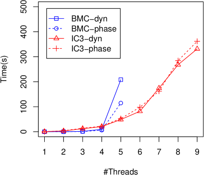
(a) Table inserts

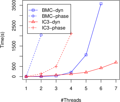
(b) Table lookups

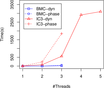
(c) Table inserts / lookups

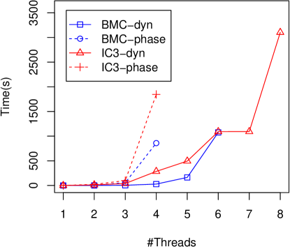
(d) Dynamic locking

Figure 10: Hash table and dynamic locking benchmark results

Dynamic locking

To study the effect of lock pointer analysis, we use a benchmark in which multiple threads use a common lock to access two global variables. The single lock these threads use is randomly picked from a set of locks at the beginning of the program. Each thread writes the same value four times to both global variables. Because all threads use the same lock, after all threads terminate, the value of both global variables must be the same, which is the verification condition. We use our static pointer heuristic to determine that all global variable accesses are protected by the same lock, potentially allowing the critical section to become a single transaction. fig:dynlock shows that the dynamic reduction indeed kicks in and benefits both IC3 and BMC.

Load balancing

We use the load-balancing example (ex:pointers). It relies on the static pointer heuristic. We verified that the computed sum of the counters is indeed the expected result. Our experiment revealed that dynamic reductions reduce the runtime from 15 minutes to 97 seconds for two threads already.

SVComp

We also ran our IC3 implementation on the pthread-ext and pthread-atomic categories of the software verification competition (SVComp) benchmarks [4, 2]. In instances with an unbounded number of threads, we introduced a limit of three threads. To check the effect of different reduction-strategies on the verification time, we tested the following reductions:

dyn:

Dynamic with all heuristics from tab:heuristics.

phase:

Dynamic phases only (equal to [17]).

static:

Static (as in sec:prelim).

nored:

No reduction, all interleavings considered.

fig:svcomp shows that static Lipton reduction yields an average six-fold decrease in runtime when compared to no reduction. Enabling the various dynamic improvements (dyn, phase) does not show improvement over the static case (static), since most of the benchmarks are either too small or do not have opportunities for reductions, but also not much overhead (up to $7\%$). Comparing the nored case with the other cases shows the benefit of removing intermediate states.

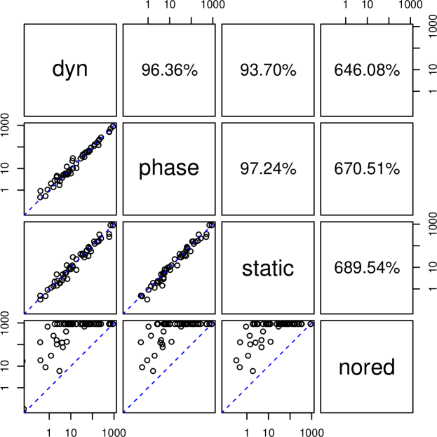
Figure 11: Scatterplots comparing runtimes for all combinations of reduction variants on SVComp benchmarks. The upper half shows relative accumulated runtimes for these combinations.

7 Related Work

Lipton’s reduction was refined multiple times [31, 20, 13, 11, 40]. It has recently been applied in the context of compositional verification [39]. Qadeer and Flanagan proposed reductions with dynamic phases [17] using phase variables to identify internal and external states and also provided a dynamic solution for determining locked regions. Their approach, however, does not solve the examples featured in the current paper and also relies on a specialized deductions incompatible with IC3. Moreover, in [17], the phases of target locations of non-deterministic conditions are required to agree. This restriction is not present in our encoding.

Grumberg et al. [21] present underapproximation-widening, which iteratively refines an under-approximated encoding of the system. In their implementation, interleavings are constrained to achieve the under-approximation. Because refinement is done based on verification proofs, irrelevant interleavings will never be considered. The technique currently only supports BMC and the implementation is not available, so we did not compare against it.

Kahlon et al. [27] extend the dynamic solution of [17], by supporting a strictly more general set of lock patterns. They incorporate the transactions into the stubborn set POR method [42] and encode these in the transition relation in similar fashion as in [1]. Unlike ours, their technique does not support other constructs than locks.

While in fact it is sufficient for item2:postterm of def:pas2 to pinpoint a single state in each bottom SCC of the CFG, we use feedback sets because the encoding in sec:encoding also requires them. Moreover, we take a syntactical definition for ease of explanation. Semantic heuristics for better feedback sets can be found in [29] and can easily be supported via state predicates. (Further optimizations are possible [29].) Obtaining the smallest (vertex) LFS is an -complete problem well known in graph theory [8]. As CFGs are simple graphs, estimations via basic DFS suffice. (In POR, similar approaches are used for the ignoring problem [43, 35].)

Elmas et al. [15] propose dynamic reductions for type systems, where the invariant is used to weaken the mover definition. The over-approximations performed in IC3, however, decrease the effectiveness of such approaches.

In POR, similar techniques have been employed in [14] and the earlier-mentioned necessary enabling sets of [19, 41]. Completely dynamic approaches exist [16], but symbolic versions remain highly static [1]. Notable exceptions are peephole and monotonic POR by Wang et al. [44, 28]. Like sleep sets [19], however, these only reduce the number of transitions—not states—which is crucial in e.g. IC3 to cut counterexamples to induction [9]. Cartesian POR [22] is a dynamic form of Lipton reduction for explicit-state model checking.

8 Conclusions

Our work provides a novel dynamic reduction for symbolic software model checking. To accomplish this, we presented a reduction theorem generalized with bisimulation, facilitating various dynamic instrumentations as our heuristics show. We demonstrated its effectiveness with an encoding used by the BMC and IC3 algorithms in VVT.

Appendix 0.A Dynamic Reduction

The current appendix provides proofs for sec:dynamic. Some definitions presented here are more general in that they support both dynamic right and left movers, whereas sec:dynamic only considers dynamic both movers for ease of explanation. The instrumentation is consequently also adapted to support dynamic left and right movers. Moreover, def:pas2 is decomposed into def:pas, def:tas and def:errors in order to introduce these concepts in a top-down, incremental fashion. Several lemmas are proved along the way, to finally conclude soundness and completeness of the axiomatized reduction in th:soundandcomplete.

lem:instrument goes on to show that our instrumentation preserves errors. And, lem:instrument2 shows that it fulfills the reduction axioms. So the instrumentation can be used as a valid basis for obtaining reductions.

The inspiration for our reduction theorem comes from [17], which in turn is based on a string of earlier works (see sec:related). Its generalization with bisimulation is necessary to accommodate the dynamic behavior of movers, which causes entire atomic sections to “switch phase” as explained in sec:reduction.

Definition 6 (phase-annotated transition system).

A parallel phase-annotated transition system ${PT}_{TS}$ is a transition system ${TS}=\left(S,\rightarrow\right)$ with a (parallel) transition relation $\rightarrow=\bigcup_{i}\rightarrow_{i}$ whose states are partitioned in three sets (of phases), for each thread $i$, and for all threads $i$ there exists a thread bisimulation $\cong_{i}$. Additionally, we require the following properties (for all $i$ and all $j\neq i$):

1. $S=\mathcal{R}_{i}\uplus\mathcal{L}_{i}\uplus\mathcal{N}_{i}$ (the 3-partition)

2. $\rightarrow_{i}\cap\rightarrow_{j}=\emptyset$ ($i$’s and $j$’s transitions are disjoint)

3. $\rightarrow_{i}\,\subseteq\mathcal{\mathcal{L}}_{j}^{2}\cup\mathcal{\mathcal{R}}_{j}^{2}\cup\mathcal{\mathcal{N}}_{j}^{2}$ ($i$ preserves $j$’s phase)

4. $\cong_{i}\,\subseteq\mathcal{\mathcal{L}}_{j}^{2}\cup\mathcal{\mathcal{R}}_{j}^{2}\cup\mathcal{\mathcal{N}}_{j}^{2}$ ($\cong_{i}$ preserves phase-equality for $j$)

Note that all transitions in a parallel phase-annotated transition system are distinguishable, i.e., can be assigned to unique threads performing them (due to the parallel transition relation property and item:disjoint). We will apply this feature silently and assign threads to steps in paths whenever needed.

We next define equivalence relations $\cong_{X}$ for $X\subseteq\mathsf{Threads}$ and let $\cong\,\triangleq\,\cong_{\mathsf{Threads}}$. We put

$$\cong_{X}=\left(\bigcup_{i\in X}\cong_{i}\right)^{*}.$$

Hence, $\cong_{X}$ is the equivalence closure of the union of all $\cong_{i}$. Note that (1) $\cong_{\{i\}}=\cong_{i}$, and (2) $\cong_{X}\subseteq\mathcal{\mathcal{L}}_{j}^{2}\cup\mathcal{\mathcal{R}}_{j}^{2}\cup\mathcal{\mathcal{N}}_{j}^{2}$ for all $j\notin X$. The following properties are immediate.

Corollary 2.

The relation $\cong_{X}$ is a thread bisimulation. As a consequence, it is also a standard bisimulation of $(S,\rightarrow)$.

Corollary 3.

For any path starting in $\sigma$, if $\sigma^{\prime}$ is such that $\sigma^{\prime}\cong_{X}\sigma$ for $X\subseteq\mathsf{Threads}$, then there is a (bisimilar) path from $\sigma^{\prime}$ where the same threads transit in the same order.

Corollary 4.

For a path $\sigma_{1}\rightarrow\sigma_{2}\rightarrow\ldots$, let the phase trace for $i$ be a sequence $X_{1},X_{2},\ldots$ with $X_{x}=\mathcal{R}\Leftrightarrow\sigma_{x}\in\mathcal{R}_{i}$, etc. Bisimilar states $\sigma\cong_{X}\sigma^{\prime}$ have equal phase traces for all $i$ such that $i\notin X$.

Let $\mathcal{N}_{T}\,\triangleq\,\bigcap_{i\in T}\mathcal{N}_{i}$ and $\mathcal{N}=\mathcal{N}_{\mathsf{Threads}}$.

Definition 7 (parallel transaction system).

A parallel transaction system ${TS}_{TS}$ is a phase-annotated transition system ${PT}_{TS}\,\triangleq\,(S,\rightarrow)$ s.t. for all $i$ and all $j\neq i$:

1. $\mathcal{\mathcal{L}}_{i}\mathrel{\reflectbox{\rotatebox[origin={tr}]{25.0}{$\|$}}}\rightarrow_{i}\mathrel{\reflectbox{\rotatebox[origin={tl}]{-25.0}{$\|$}}}\mathcal{\mathcal{R}}_{i}=\emptyset$ ((locally) post does not reach pre)

2. $(\rightarrow_{i}\mathrel{\reflectbox{\rotatebox[origin={tl}]{-25.0}{$\|$}}}\mathcal{R}_{i})\stackrel{{\scriptstyle\rightarrow}}{{\bowtie}}_{j}\rightarrow_{j}$ ($i$ to pre right commutes up to $j$ with $j$)

3. $(\mathcal{L}_{i}\mathrel{\reflectbox{\rotatebox[origin={tr}]{25.0}{$\|$}}}\rightarrow_{i})\stackrel{{\scriptstyle\leftarrow}}{{\bowtie}}_{\left\{i,j\right\}}\rightarrow_{j}$ ($i$ from post left commutes up to $\{i,j\}$ with $j$)

4. $\forall\sigma\in\mathcal{L}_{i}\colon\exists\sigma^{\prime}\in\mathcal{N}_{i}\colon\sigma\rightarrow_{i}^{+}\sigma^{\prime}$ (post phases terminate)

The transaction relation is $\hookrightarrow=\bigcup_{i}\hookrightarrow_{i}$ with

$\hookrightarrow_{i}\,\triangleq\,\mathcal{N}_{j\neq i}\mathrel{\reflectbox{\rotatebox[origin={tr}]{25.0}{$\|$}}}\rightarrow_{i}$   ($i$ only transits when all $j$ are in external).

th:dynred shows that for all paths in a transaction system there also exists a bisimilar transaction path ($\hookrightarrow$). This enables reduction by removing interleavings. But first, we prove several intermediate lemmas, before we can introduce the error states used in the theorem to connect divergent paths between the two transition relations.

The above definition differs on some key points from that of Flanagan and Qadeer: Most importantly, it lifts the commutativity condition from the phase change. This means that while transitions should still commute, their phase change might not, crucially enabling the dynamic instrumentation. To preserve correctness while allowing phase changes when moving transitions, the system is constructed in such a way that these phase-unequal states are still bisimilar as the above corollaries demonstrate.

0.A.1 Incomplete Transaction Paths

To reason over (transaction) paths where some threads are still in the middle of their transaction (open), we introduce the notion of open transaction sequences (ots). An ots consists of two concatenated subpaths: The first (called cts) has only transactions in committed form (ending in post-commit or external phase), while the second (called uts) only contains uncommitted transitions (ending in the pre-commit phase). For example, the phase trace for 3 different threads of the same path could look like:

1: NNNRRLLLNRRLLLLLLNNNNNNNNNNnRRRRRR
2: NNNNNNNNNNNNNNNNNNRRRRRLLLLnNNNNRR
3: NLLLLLLLLLLLLLLLLLLLLLLLLLLLLLLLLL

Here the small letters indicate phases of states that are part of both the cts (where it is the last state of the cts) and the uts (the first state). We start with a definition of the uts, as it is easier to understand. We also prove two lemmas that are needed for correctness of the reduction in s:theorem.

Definition 8 (Uncommitted transaction sequence (uts)).

A uts under a set of threads $T$ is a sequence of transactions

$$q=q_{1}\rightarrow_{\psi(1)}^{+}q_{2}\rightarrow_{\psi(2)}^{+}\ldots\rightarrow_{\psi(l)}^{+}q_{l+1}$$

(where $l\geq 0$ and $\psi$ is a mapping from indices to threads) such that for all $1\leq i\leq l$, we have

$$q_{i}=q_{i,1}\rightarrow_{\psi(i)}\ldots\rightarrow_{\psi(i)}q_{i,x_{i}}=q_{i+1}$$

with

1. $\psi(i)\in T$ and $q_{1}\in\mathcal{N}_{T}$,

2. $q_{i,1}\in\mathcal{N}_{\psi(i)}$, and

3. $q_{i,2},\ldots,q_{i,x_{i}}\in\mathcal{R}_{\psi(i)}$.

Corollary 5.

For every uts as defined in def:uts it holds that

$$\forall i,j\in\{1,\dots,l\}\colon i\neq j\Rightarrow\psi(i)\neq\psi(j)\,.$$

Corollary 6.

Every uts $q_{1}\rightarrow_{\psi(1)}^{+}q_{2}\rightarrow_{\psi(2)}^{+}\ldots\rightarrow_{\psi(l)}^{+}q_{l+1}$ under $T$ can be split at an arbitrary index $1\leq k\leq l+1$ into two uts’s:
$q_{1}\rightarrow_{\psi(1)}^{+}\ldots\rightarrow_{\psi(k-1)}^{+}q_{k}$ , a uts under $T$, and
$q_{k}\rightarrow_{\psi(k)}^{+}\ldots\rightarrow_{\psi(l)}^{+}q_{l+1}$ , a uts under $\left\{i\in T\mid q_{k}\in\mathcal{N}_{i}\right\}$.

Lemma 4.

Given a uts $q_{1}\rightarrow_{\psi(1)}^{+}q_{2}\rightarrow_{\psi(2)}^{+}\ldots\rightarrow_{\psi(l)}^{+}q_{l+1}$ under $T_{u}\,\triangleq\,\mathit{range}(\psi)$ and a transition $q_{l+1}\rightarrow_{i}q$ with $i\not\in T_{u}$, then there exists a transition $q_{1}\rightarrow_{i}q^{\prime}$ and a uts $q^{\prime}=q_{1}^{\prime}\rightarrow_{\psi(1)}^{+}q_{2}^{\prime}\allowbreak\rightarrow_{\psi(2)}^{+}\ldots\rightarrow_{\psi(l)}^{+}q_{l+1}^{\prime}$ under $T_{u}$ such that $q_{l+1}^{\prime}\cong_{\left\{i\right\}}q$. Illustratively:

Proof.

The proof proceeds by nested induction over the transaction blocks in the uts and the steps inside each block.

The outer induction is performed over the length $l$ (i.e., the number of transactions) of the uts.

• Base case ($l=0$): Choose $q_{1}^{\prime}=q_{l+1}^{\prime}=q^{\prime}$, which is trivially a uts of length 0. Furthermore, $q_{l+1}^{\prime}\cong q$.

• Induction hypothesis (IH): Suppose that the lemma holds for the sequence

  $$q_{1}\rightarrow_{\psi(1)}^{+}q_{2}\rightarrow_{\psi(2)}^{+}\ldots\rightarrow_{\psi(l-1)}^{+}q_{l}\rightarrow_{i}q$$

  (or $q_{1}(\rightarrow^{+})^{l-1}q_{l}\rightarrow_{i}q$, for short).

• Inductive case: Using the induction hypothesis for the uts $q_{1}(\rightarrow^{+})^{l-1}q_{l}$ of length $l-1$, we show that the lemma must hold equally for a sequence

  $$\underbrace{q_{1}(\rightarrow^{+})^{l-1}q_{l}\rightarrow_{\psi(l)}^{+}q_{l+1}}_{\text{uts}}\rightarrow_{i}q^{\prime}$$

  (where also $\psi(l)\neq i$).

  Let $j\,\triangleq\,\psi(l)$ be the last thread executing before $i$. We thus have (gray parts are the proof obligation):
  

  The nested induction is over the steps in the transaction $\rightarrow_{j}^{+}$. By induction over the length $m$ of the path $q_{l}=q_{l,1}\rightarrow_{j}\ldots\rightarrow_{j}q_{l,m}=q_{l+1}$ with $q_{l,2},\ldots,q_{l,m}\in\mathcal{R}_{j}$, we show that there is a path $q_{l,1}\rightarrow_{i}q_{l,1}^{\prime}\rightarrow_{j}\ldots\rightarrow_{j}q_{l,m}^{\prime}$ with $q_{l,2}^{\prime},\ldots,q_{l,m}^{\prime}\in\mathcal{R}_{j}$ and $q_{l,m}^{\prime}\cong_{i}q^{\prime}$, if there is a transition $q_{l,m}\rightarrow_{i}q^{\prime}$:

  • Base case ($m=2$ and $q_{l,1}\rightarrow_{j}q_{l,m}\rightarrow_{i}q^{\prime}$): By item:rmover of the definition of transaction systems (def:tas), we obtain $q_{l,1}\rightarrow_{i}q_{l,1}^{\prime}\rightarrow_{j}q_{l,2}^{\prime}$ with $q_{l,2}^{\prime}\cong_{\left\{i\right\}}q^{\prime}$ and $q_{l,2}^{\prime}\in\mathcal{R}_{j}$.

  • Induction hypothesis (IH2): Assume that the hypothesis holds for $(m-1)>0$.

  • Induction step: We show that our claim holds for a path up to $m$ ending with: $q_{l,m-1}\rightarrow_{j}q_{l,m}\rightarrow_{i}q^{\prime}$ with $q_{l,m}\in\mathcal{R}_{j}$. By item:rmover of def:tas, we obtain $q_{l,m-1}\rightarrow_{i}q_{l,m-1}^{\prime}\rightarrow_{j}q_{l,m}^{\prime}$ with $q_{l,m}^{\prime}\cong_{\left\{i\right\}}q^{\prime}$ and $q_{l,m}^{\prime}\in\mathcal{R}_{j}$. We then apply IH2 on the path of length $m-1$ to obtain a path $q_{l,1}\rightarrow_{i}q_{l,1}^{\prime}\rightarrow_{j}\ldots\rightarrow_{j}q_{l,m-2}^{\prime}\rightarrow_{j}q_{l,m-1}^{\prime\prime}$ with $q_{l,2}^{\prime},\ldots,q_{l,m-1}^{\prime}\in\mathcal{R}_{j}$ and $q_{l,m-1}^{\prime\prime}\cong_{\left\{i\right\}}q_{l,m-1}^{\prime}$. This implies $q_{l,m-1}^{\prime\prime}\rightarrow_{j}q_{l,m}^{\prime\prime}$ with $q_{l,m}^{\prime}\cong_{\left\{i\right\}}q_{l,m}^{\prime\prime}$ (since $\cong_{\left\{i\right\}}$ is a bisimulation relation). Since $\cong_{\left\{i\right\}}$ preserves the phase of other threads, it follows that $q_{l,m}^{\prime\prime}\in R_{j}$ from $q_{l,m}^{\prime}\in R_{j}$.

    The resulting path satisfies the required property. Note that $q_{l,1}^{\prime}\rightarrow_{j}\ldots\rightarrow_{j}q_{l,m}^{\prime}$ is a uts.

  We thus obtain a transition sequence:

  $$\underbrace{q_{1}\rightarrow_{\psi(1)}^{+}\ldots\rightarrow_{\psi(l-1)}^{+}q_{l}\rightarrow_{i}q_{l}^{\prime}}_{A}{\rightarrow_{\psi(l)^{+}}q_{l+1}^{\prime}}$$

  with $\psi(1),\ldots,\psi(l-1)\neq i$. Applying the IH to $A$ yields a path:

  $$q_{1}\rightarrow_{i}\underbrace{q_{1}^{\prime}\rightarrow_{\psi(1)}^{+}q_{2}^{\prime}\rightarrow_{\psi(2)}^{+}\ldots q_{l-1}^{\prime}\rightarrow_{\psi(l-1)}^{+}q_{l}^{\prime\prime}}_{B}$$

  Since, $q_{l}^{\prime}\cong_{\left\{i\right\}}q_{l}^{\prime\prime}$, we also have $q_{l}^{\prime\prime}\rightarrow_{j}q_{l+1}^{\prime\prime}$, by cor:bisim-threads and $i\neq j$. This is a uts under $\left\{j\right\}$. Since $B$ remains a uts under $T_{u}$, the path $q_{1}^{\prime}(\rightarrow^{+})^{n}q_{l+1}^{\prime}$ satisfies the needed property (it is a uts under $T_{u}\uplus\left\{j\right\}$).

∎

Definition 9 (Committed transaction sequence (cts)).

A cts under $T\subseteq\mathsf{Threads}$ is a sequence of transactions with $k\geq 0$:

$$p=p_{1}\rightarrow_{\varphi(1)}^{+}p_{2}\rightarrow_{\varphi(2)}^{+}\ldots\rightarrow_{\varphi(k)}^{+}p_{k+1}$$

such that for all $1\leq i\leq k$, we have $p_{i}=p_{i,1}\rightarrow_{\varphi(i)}\ldots\rightarrow_{\varphi(i)}p_{i,x_{i}}=p_{i+1}$ with

1. $\varphi(i)\in T$ and $p_{1}\in N_{T}$,

2. $p_{i,1}\in\mathcal{N}_{\varphi(i)}$,

3. $p_{i,2},\ldots,p_{i,x_{i}-1}\in\mathcal{R}_{\varphi(i)}\cup\mathcal{L}_{\varphi(i)}$, and

4. $p_{i,x_{i}}\in\mathcal{L}_{\varphi(i)}\cup\mathcal{N}_{\varphi(i)}$.

Corollary 7.

An analogous “splitting” property to the one from cor:split-uts also holds for cts’s.

Definition 10 (Open transaction sequence (ots)).

If $A$ is a cts under $T_{A}$ and $B$ is a uts under $T_{B}$ such that $A$ ends in the same state in which $B$ starts, then the sequence of transactions $A\circ B$ obtained by appending $B$ to $A$ is an ots under $T_{A}\cup T_{B}$.

We sometimes write $AB$ for $A\circ B$. We refer to the cts part of $AB$ by using states $p_{x},p_{x+1}$ (transactions start/end states), $p_{x,y},p_{x,y+1}$ (internal transitions) and threads $\varphi(x)$ for a transaction index $x$ and an internal transition index $y$ (as in def:cts). Similarly, we refer to the uts part by using states $q_{x},q_{x+1}$ (transactions start/end states), $q_{x,y},q_{x,y+1}$ (internal transitions) and threads $\psi(x)$ for a transaction index $x$ and an internal transition index $y$ (as in def:uts).

Corollary 8.

For an ots containing a sub-trace $\ldots r\rightarrow_{i}\ldots$ with $r\notin\mathcal{N}_{j}$ for $j\neq i$, the suffix from $r$ does not contain $j$ transitions.

Corollary 9.

An analogous “splitting” property to the one from cor:split-uts also holds for ots’s.

Corollary 10.

Every path $p\rightarrow_{i}^{*}q$ with $p\in\mathcal{N}_{i}$ in a transaction system is an ots under $\{i\}$.

Lemma 5 (From transaction system path to ots).

Let ${TS}$ be a transaction system and $\rightarrow_{T}\,\triangleq\,\bigcup_{i\in T}\rightarrow_{i}$.

Suppose that $p\rightarrow^{*}_{T}q$ is a ${TS}$ path with $p\in\mathcal{N}_{T}$, then there exists an ots $p\rightarrow^{*}q^{\prime}$ under $T$ s.t. $q^{\prime}\cong q$.

Proof.

We prove the hypothesis by induction on the length of the path $p\rightarrow^{*}q$. The induction hypothesis (IH) is:

For every path $p\rightarrow_{T}^{*}q$ with $p\in\mathcal{N}_{T}$ there is a path

$$p=\underbrace{p_{1}\rightarrow_{\varphi(1)}^{+}p_{2}\ldots p_{k+1}}_{A}=\underbrace{q_{1}\rightarrow_{\psi(1)}^{+}q_{2}\ldots q_{l}\rightarrow_{\psi(l)}^{+}q_{l+1}}_{B}$$

such that $q_{l+1}\cong q$, $A$ is a cts under $T_{C}\,\triangleq\,\mathit{range}(\varphi)$, and $B$ a uts under $T_{U}\,\triangleq\,\mathit{range}(\psi)$ (so that $AB$ is an ots under $T_{C}\cup T_{U}\subseteq T$).

For the base case, $k=l=0$, take $q^{\prime}\,\triangleq\,p=q$ and the conclusion holds trivially. Let $p\rightarrow^{*}q\rightarrow_{i}r$ be the path extension with $i$, so the IH holds for $p\rightarrow^{*}q$. We show that there is an $r^{\prime}\cong r$ and a path $p\rightarrow^{+}r^{\prime}$ that is an ots (under $T_{C}\cup T_{U}\cup\{i\}$).

We do case analysis over the $i$-phase of $q$:

$q\in\mathcal{N}_{i}$:

It follows that $i\not\in T_{U}$, because otherwise we would have $q\in\mathcal{R}_{i}$ (by an inductive argument using the definition of the uts and item:invar of def:pas, also needed in the proof of cor:suffix). Using lemma:right-move-uts, one can move the transition to the end of the cts phase:

$$\underbrace{p_{1}\rightarrow_{\varphi(1)}^{+}\ldots\rightarrow_{\varphi(k)}p_{k+1}}_{\mathrm{cts}}\rightarrow_{i}\underbrace{q_{1}^{\prime}\rightarrow_{\psi(1)}^{+}\ldots\rightarrow_{\psi(l)}^{+}q_{l+1}^{\prime}}_{\mathrm{uts}}$$

such that $q_{l+1}^{\prime}\cong_{\left\{i\right\}}q_{l+1}$. Depending on the phase of transition $i$’s target state $q_{1}^{\prime}$, the transition can either be part of the cts ($q_{1}^{\prime}\in\mathcal{N}_{i}$ or $q_{1}^{\prime}\in\mathcal{L}_{i}$) or of the uts ($q_{1}^{\prime}\in\mathcal{R}_{i}$). We pick $r^{\prime}\,\triangleq\,q^{\prime}_{l+1}$. By lemma:right-move-uts, we have $r^{\prime}\cong_{\left\{i\right\}}r$. The new path has the same transitions as the original path plus $i$ (if $i$ was not in the path of the induction hypothesis). Hence, the property is satisfied.

$q\in\mathcal{L}_{i}$:

As in the previous case, we have $i\not\in T_{U}$. There is at least one $x$ such that $\varphi(x)=i$, otherwise we would have $q\in\mathcal{N}_{i}$ (again applying the same inductive reasoning over the cts prefix path). Let $x$ be largest index for which $\varphi(x)=i$, so that $\rightarrow_{\varphi(x)}$ is the rightmost occurrence of $i$ in the ots. Therefore, the path has the form:

$$p_{1} \rightarrow_{\varphi(1)}^{+}\ldots p_{x}\rightarrow_{\varphi(x)}^{+}p_{x+1}\ldots\rightarrow_{\varphi(k)}^{+}p_{k+1}=q_{1}$$

$$\rightarrow_{\psi(1)}^{+}\ldots\rightarrow_{\psi(l)}^{+}q_{l+1}=q\rightarrow_{i}r.$$

Using item:lmover from def:tas, one can construct a path

$$p_{1}\rightarrow_{\varphi(1)}^{+}\ldots\rightarrow_{\varphi(x-1)}^{+}p_{x}\rightarrow_{\varphi(x)}^{+}p_{x+1}\rightarrow_{i}\underbrace{p_{x+1}^{\prime}\rightarrow^{*}q^{\prime}}_{A}$$

with $q^{\prime}\cong r$. By cor:split-cts, the prefix path including $p_{x+1}$ is a cts, so the prefix path including $p_{x+1}^{\prime}$ is also a cts. Moreover, since by cor:split-ots the original suffix path $p_{x+1}\rightarrow^{*}q$ is an ots under $T^{\prime}$ for some $T^{\prime}\subseteq T\setminus\left\{i\right\}$, the threads that transit in $A$ are still those in $T^{\prime}$ by virtue of item:lmover and cor:bisim-threads. By contraposition of cor:suffix, we also have $p_{x+1}\in\mathcal{N}_{T^{\prime}}$ and therefore also $p_{x+1}^{\prime}\in\mathcal{N}_{T^{\prime}}$ (by item:invar of def:pas and $i\notin T^{\prime}$).

Since $1\leq x\leq k$, the suffix path $A$ is shorter than the original path. Hence one can apply the (strong) induction hypothesis to $A$ with $T^{\prime}$ to obtain an ots under $T^{\prime}$ starting in $p^{\prime}_{x+1}\in\mathcal{N}_{T^{\prime}}$. This yields an ots under $T$:

$$\overbrace{p_{1}\rightarrow_{\varphi(1)}^{+}\ldots\rightarrow_{\varphi(x-1)}^{+}p_{t}\rightarrow_{\varphi(t)}^{+}p_{x+1}\rightarrow_{i}\underbrace{p_{x+1}^{\prime}\rightarrow^{*}_{T^{\prime}}q^{\prime\prime}}_{\text{ots under}~{}T^{\prime}}}^{\text{ots under}~{}T}$$

with $q^{\prime\prime}\cong q^{\prime}$. Let $r^{\prime}\,\triangleq\,q^{\prime\prime}$. By transitivity of $\cong$, we have $r^{\prime}\cong r$. Thus the property is satisfied.

$q\in\mathcal{R}_{i}$:

There is at least one $x$ such that $\psi(x)=i$, otherwise we would have $q\in\mathcal{N}_{i}\cup\mathcal{L}_{i}$ (again applying the same inductive reasoning over the ots). Let $x$ be the largest index for which $\psi(x)=i$, so that $\rightarrow_{\psi(x)}$ is the rightmost occurrence of $i$ in the ots.

One can then split the path into a cts $A$ under $T$ (cor:split-uts), a uts $B$ under $T_{B}\subseteq T$ and a uts $C$ under $T_{C}=T\setminus T_{B}$ by cor:uts-threads:

$$\underbrace{p_{1}\rightarrow_{\varphi(1)}^{+}\ldots\rightarrow_{\varphi(k)}p_{k+1}}_{A}$$

$$=\underbrace{q_{1}\rightarrow_{\psi(1)}^{+}\ldots q_{x}\rightarrow_{\psi(x)}^{+}q}_{B}\underbrace{{}_{x+1}\ldots\rightarrow_{\psi(l)}^{+}q_{l+1}}_{C}\rightarrow_{i}r$$

From the above, we have $i\in T_{B}$, but $i\notin T_{C}$. Hence, one can apply lemma:right-move-uts to $C$ and $i$ to obtain a uts $C^{\prime}$ under $T_{C}$ (ignore $D$ for now):

$$\underbrace{p_{1}\rightarrow_{\varphi(1)}^{+}\ldots\rightarrow_{\varphi(k)}p_{k+1}}_{A}=\underbrace{\overbrace{q_{1}\rightarrow_{\psi(1)}^{+}\ldots q_{x}}^{D}\rightarrow_{\psi(x)}^{+}q_{x+1}}_{B}$$

$$\rightarrow_{i}\underbrace{q_{x+1}^{\prime}\ldots\rightarrow_{\psi(l+1)}^{+}q_{l+1}^{\prime}}_{C^{\prime}}=r^{\prime}\cong_{i}r$$

If $q_{x+1}^{\prime}\in\mathcal{R}_{i}$, we are done as this path is an ots (under $T\ni i$). Otherwise, by repeatedly applying lemma:right-move-uts to the each of the $i$-transitions $q_{x}\rightarrow_{i}^{+}q^{\prime}_{x+1}$ and $D$ (a path without $i$), we right-commute all $i$-transitions to the end of the cts:

$$\overbrace{\underbrace{p_{1}\rightarrow_{\varphi(1)}^{+}\ldots\rightarrow_{\varphi(k)}p_{k+1}}_{A}\rightarrow_{i}^{+}p_{k+1}^{\prime}}^{\text{cts under~{}}T\cup\left\{i\right\}}=\underbrace{q_{1}^{\prime}\rightarrow_{\psi(1)}^{+}\ldots q_{x}^{\prime}}_{B^{\prime}}$$

with $q_{x}^{\prime}=q_{x+1}^{\prime\prime}\cong_{\left\{i\right\}}q_{x+1}^{\prime}$. By cor:always_ots, we obtain a new cts $B^{\prime}$ under $T\cup\left\{i\right\}$. Moreover, by bisimilarity up to $i$ (cor:bisim-upto), we also have a path:

$$\underbrace{q_{x+1}^{\prime\prime}\ldots\rightarrow_{\psi(l+1)}^{+}q_{l+1}^{\prime\prime}}_{C^{\prime\prime}}=r^{\prime\prime},\quad\text{~{}with~{}}r^{\prime\prime}\cong_{i}r^{\prime}$$

This path is still a uts under $T_{C}$, because $i\notin T_{C}$. Therefore, the resulting path $p_{1}\rightarrow_{T}^{+}r^{\prime\prime}$ is an ots under $T$ with $r^{\prime\prime}\cong_{i}r$ by transitivity of $\cong_{i}$. This path satisfies the property.

Since $q\in\mathcal{R}_{i}\uplus\mathcal{L}_{i}\uplus\mathcal{N}_{i}$, our case analysis and proof is complete. ∎

0.A.2 Dynamic Reduction Theorem

We aim at preserving reachability of error states under the reduction. We require the following of error states, without loss of generality (e.g. error states can be implemented using sinks or a monitor process).

Definition 11.

Let $\mathcal{E}\,\triangleq\,\bigcup_{t}\mathcal{E}_{i}$ be error states in a transaction system, then for all $j\neq i$ and all $k$:

1. $\mathcal{E}_{i}\subseteq\mathcal{N}_{i}$ (errors are external states)

2. $\mathcal{E}_{i}\mathrel{\reflectbox{\rotatebox[origin={tr}]{25.0}{$\|$}}}\rightarrow_{i}\mathrel{\reflectbox{\rotatebox[origin={tl}]{-25.0}{$\|$}}}\overline{\mathcal{E}_{i}}=\emptyset$ (local transitions preserve errors)

3. $\rightarrow_{i}\,\subseteq\mathcal{E}_{j}^{2}\cup\overline{\mathcal{E}_{j}}^{2}$ (transitions preserves remote (non)errors)

4. $\cong_{i}\,\subseteq\mathcal{E}_{k}^{2}\cup\overline{\mathcal{E}_{k}}^{2}$ (bisimulations preserve (non)errors)

Corollary 11.

If $q\in\mathcal{E}_{i}$ for some $i$ in lem:ots, then also $q^{\prime}\in\mathcal{E}_{i}$, owing to def:errors item:errors3.

Theorem 0.A.1 (reduction of interleavings).

Let ${TS}=\left(S,\to\right)$ be a parallel transaction system as in def:tas with errors as in def:errors and $\mathcal{L}\,\triangleq\,\bigcup_{t}\mathcal{L}_{i}$.

Suppose that $p\rightarrow^{*}q$, $p\in\mathcal{N}$ and $q\in\mathcal{E}$, then there is $p\hookrightarrow^{*}q^{\prime}$ s.t. $q\cong q^{\prime}\in\mathcal{E}$.

Proof.

By lem:ots, the hypothesis implies that there is an ots under $\mathsf{Threads}$:
$p=p_{1}(\rightarrow^{+}_{T_{c}})^{*}p_{k+1}=q_{1}(\rightarrow^{+}_{T_{u}})^{*}q_{l+1}$ with $q_{l+1}\cong q$ and $T_{c}\cup T_{u}=\mathsf{Threads}$.

First, we show that there also is an ots ending in $q_{l+1}$ with $q_{l+1}\notin\mathcal{L}$. We do this by completing paths that are stuck in the post phase ($\mathcal{L}$), starting with the thread that gets stuck the first (left-most in the path). Let $x$ be the lowest index, such that there exists a subpath:

$$p_{x}\rightarrow_{\varphi(x)}^{+}p_{x+1}\rightarrow_{\varphi(x+1)}^{+}p_{x+2}\text{~{}~{}with~{}~{}}p_{x+1}\in\mathcal{L}_{\varphi(x)}$$

Let $i\,\triangleq\,\varphi(x)$. By item:invar of def:pas, this subpath must exists when $q_{l+1}\in\mathcal{L}_{i}$. Hence, by construction, we have $p_{x}\in\mathcal{N}$ (trivially from the cts definition, we have $p_{x}\in\mathcal{N}_{i}$ and for $j\neq i$ anything but $p_{x}\in\mathcal{N}_{j}$ would contradict the assumption of having chosen the lowest $x$). Also, by cor:suffix, the suffix from $p_{x+1}$ does not contain $i$ transitions.

Now we extend the path with $i$: $\mathcal{L}_{i}\ni q_{l+1}\rightarrow_{i}q^{\prime\prime}$. This is possible by item:postterm of def:tas. Using again strong induction with the same IH as in the proof of lem:ots, we may move the new $i$ transition ‘in place’ as a first step towards constructing a new ots. Thus using item:lmover from def:tas and cor:bisim-threads, one can construct a path:

$$p_{1}\rightarrow_{\varphi(1)}^{+}\ldots\rightarrow_{\varphi(x-1)}^{+}p_{x}\rightarrow_{\varphi(x)}^{+}p_{x+1}\rightarrow_{i}\underbrace{p_{x+1}^{\prime}\rightarrow^{*}q^{\prime\prime\prime}}_{A}\cong q^{\prime\prime}$$

By cor:split-cts, the prefix path including $p_{x+1}$ is a cts, so the prefix path including $p_{x+1}^{\prime}$ is also a cts (by item:post of def:tas). Moreover, since by cor:split-ots the original suffix path $p_{x+1}\rightarrow^{*}q_{l+1}$ is an ots under $T^{\prime}=\mathsf{Threads}\setminus\left\{i\right\}$. The threads that transit in $A$ are still contained in $T^{\prime}$ by virtue of item:lmover and cor:bisim-threads. Since $p_{x}\in\mathcal{N}$, we also have $p_{x+1},p_{x+1}^{\prime}\in\mathcal{N}_{T^{\prime}}$ (by item:invar of def:pas and $i\notin T^{\prime}$).

Since $1\leq x\leq k$, the suffix path $A$ is shorter than the original path. Hence one can apply the (strong) induction hypothesis to $A$ with $T^{\prime}$ to obtain an ots under $T^{\prime}$ starting in $p^{\prime}_{x+1}\in\mathcal{N}_{T^{\prime}}$. This yields a new ots under $\mathsf{Threads}$:

$$\overbrace{p_{1}\rightarrow_{\varphi(1)}^{+}\ldots\rightarrow_{\varphi(x-1)}^{+}p_{t}\rightarrow_{\varphi(t)}^{+}p_{x+1}\rightarrow_{i}\underbrace{p_{x+1}^{\prime}\rightarrow^{*}_{T^{\prime}}q^{\prime\prime\prime\prime}}_{\text{ots under}~{}T^{\prime}}}^{\text{ots under}~{}\mathsf{Threads}}$$

with $q^{\prime\prime\prime\prime}\cong q^{\prime\prime\prime}\cong q^{\prime\prime}\cong q_{l+1}\cong q$. Because the bisimilarity preserves error states, we have $q^{\prime\prime\prime\prime}\in\mathcal{E}$.

We must further have $q_{x+1}^{\prime}\in\mathcal{L}_{i}$ or $q_{x+1}^{\prime}\in\mathcal{N}_{i}$ (note that the phase may have changed compared to $q^{\prime\prime}$ by the moving operation). In the former case, we repeat this process of extending the path with $i$ until $q_{x+1}^{\prime}\in\mathcal{N}_{i}$ (since the system is finite this happens eventually). In the latter case, we are done for this $i$, because $q^{\prime\prime\prime\prime}\in\mathcal{N}_{i}$. It follows that for all other $j\notin T^{\prime}$, we also have $q^{\prime\prime\prime\prime}\in\mathcal{N}_{j}$. If $q^{\prime\prime\prime\prime}\in\overline{\mathcal{L}}$, we are done showing that there is also an ots path leading to an error without ending in a post phase. Otherwise, we pick a new left-most $x^{\prime}$ and a new $i^{\prime}$ to repeat the process. Because, the number of threads is finite, $i^{\prime}\neq i$ and $x^{\prime}>x$ this process eventually terminates.

Let $p_{1}(\rightarrow^{+}_{T_{c}})^{*}p_{k+1}=q_{1}(\rightarrow^{+}_{T_{u}})^{*}q_{l+1}\in\overline{\mathcal{L}}$ be the ots after the above extension. Since, we reduced the case to an ots where $q_{l+1}\notin\mathcal{L}$, it remains to show that there exists a transaction path $\hookrightarrow$ to some $q^{\prime}\in\mathcal{E}$. We know that $q\in\mathcal{E}_{i}\subseteq\mathcal{N}_{i}$ for some thread $i$. Therefore, we have $i\notin T_{u}$ and $q_{1}\in\mathcal{E}_{i}\subseteq\mathcal{N}_{i}$ by item:invar of def:pas. Also, because $q_{l+1}\in\overline{\mathcal{L}}$, we have $q_{1}\in\mathcal{N}$. Let $q^{\prime}\,\triangleq\,q_{1}=p_{k+1}$. It is easy to show that the this cts is also a $\bigcup_{i}\hookrightarrow_{i}$ path. Hence, the conclusion is satisfied. ∎

The following theorem shows that internal states may just as well be skipped. This theorem is found in sec:dynamic as th:blockred.

Theorem 0.A.2 (Atomic block reduction).

The block-reduced transition relation is defined as:

$$\leadsto_{i}\,\triangleq\,\mathcal{N}_{i}\mathrel{\reflectbox{\rotatebox[origin={tr}]{25.0}{$\|$}}}(\hookrightarrow_{i}\mathrel{\reflectbox{\rotatebox[origin={tl}]{-25.0}{$\|$}}}\overline{\mathcal{N}_{i}})^{*}\hookrightarrow_{i}\mathrel{\reflectbox{\rotatebox[origin={tl}]{-25.0}{$\|$}}}\mathcal{N}_{i}\text{~{}~{}and~{}~{}}\leadsto\,\triangleq\,\bigcup_{i}\leadsto_{i}$$

There is path $p\rightarrow^{*}q$, $p\in\mathcal{N}$ and $q\in\mathcal{E}$, then there is $p\leadsto^{*}q^{\prime}$ s.t. $q\cong q^{\prime}\in\mathcal{E}$.

Proof.

By th:dynred, the premise gives us that there is a transaction path $p\hookrightarrow^{*}q^{\prime\prime}$ s.t. $q\cong q^{\prime\prime}\in\mathcal{E}$. We induce backwards over that transaction path to show that it is a block transition path $\leadsto$. Let $x$ be an index s.t. the path contains a transition $p_{x}\hookrightarrow_{i}p_{x+1}$ with $p_{x}\notin\mathcal{E}$ and $p_{x+1}\in\mathcal{E}$. We have $p_{x+1}\in\mathcal{E}_{i}\subseteq\mathcal{N}_{i}$, or else a contradiction with item:invar (invariance). By definition of $\rightarrow$, we also have $p_{x+1}\in\mathcal{N}$ and $p_{x}\in\mathcal{N}_{\mathsf{Threads}\setminus\left\{i\right\}}$ by invariance. If $p_{x}=p$, we are done since with $p\in\mathcal{N}$ this is a block transition ($\leadsto$). Else either $p_{x}\in\mathcal{N}_{i}$, and again we have a block transition or not. In the first case, we repeat the process until eventually we hit $p_{z}=p$ with $z<x$. In the letter case, there exists a $y<x$ s.t. $p_{y}\in\mathcal{N}$ and all intermediate states in $\mathcal{N}_{\mathsf{Threads}\setminus\left\{i\right\}}$ by invariance. Clearly, this is also a block transition step and one can repeat the process until we find some $p_{z}=p$ with $z<y$. Taking $q^{\prime}\,\triangleq\,p_{x+1}$ therefore satisfies the induction hypothesis. ∎

Theorem 0.A.3 (th:blockred in the main part).

Dynamic transaction reduction is sound and complete for the reachability of error states.

Proof.

Completeness (no error states are missed) follows from th:dynred(/th:blockred2). Soundness (no errors are introduced) follows immediately from the fact that the reduced transition relation of def:tas is a subset of the original transition relation $\rightarrow$ (and the reduced relations of th:blockred2 are subsets of the closure of the original transition relation: $\rightarrow^{+}$). ∎

0.A.3 Instrumentation

First, we define sufficient criteria for dynamic moving conditions as a simple interface to easily design other heuristics. Then we give a formal definition of the heuristics discussed in s:dyn-movers and show that they satisfy the critaria.

Definition 12 (Dynamic moving conditions).

A state predicate (a subset of states) $c^{L}_{\alpha}$ is a dynamic left-moving condition for a CFG edge $\left(l,\alpha,l^{\prime}\right)\in\delta_{i}$, if for all $j\neq i$, $\beta\in\Delta_{j}$: $(c^{L}_{\alpha}\mathrel{\reflectbox{\rotatebox[origin={tr}]{25.0}{$\|$}}}{\,}{\mathchoice{\raisebox{-3.0pt}{ $\xrightarrow{\alpha}$ }}{\raisebox{-3.0pt}{ $\xrightarrow{\alpha}$ }}{\raisebox{-3.0pt}{ $\xrightarrow{\alpha}$ }}{\raisebox{-3.0pt}{ $\xrightarrow{\alpha}$ }}_{i}}{\,\hskip 0.28453pt})\stackrel{{\scriptstyle\leftarrow}}{{\bowtie}}(c^{L}_{\alpha}\mathrel{\reflectbox{\rotatebox[origin={tr}]{25.0}{$\|$}}}{\,}{\mathchoice{\raisebox{-3.0pt}{ $\xrightarrow{\beta}$ }}{\raisebox{-3.0pt}{ $\xrightarrow{\beta}$ }}{\raisebox{-3.0pt}{ $\xrightarrow{\beta}$ }}{\raisebox{-3.0pt}{ $\xrightarrow{\beta}$ }}_{j}}{\,\hskip 0.28453pt})$ and ${\,}{\mathchoice{\raisebox{-3.0pt}{ $\xrightarrow{\beta}$ }}{\raisebox{-3.0pt}{ $\xrightarrow{\beta}$ }}{\raisebox{-3.0pt}{ $\xrightarrow{\beta}$ }}{\raisebox{-3.0pt}{ $\xrightarrow{\beta}$ }}_{j}}{\,\hskip 0.28453pt}$ preserves $c_{\alpha}={\mathrm{true}}$, i.e. $c^{L}_{\alpha}\mathrel{\reflectbox{\rotatebox[origin={tr}]{25.0}{$\|$}}}{\,}{\mathchoice{\raisebox{-3.0pt}{ $\xrightarrow{\beta}$ }}{\raisebox{-3.0pt}{ $\xrightarrow{\beta}$ }}{\raisebox{-3.0pt}{ $\xrightarrow{\beta}$ }}{\raisebox{-3.0pt}{ $\xrightarrow{\beta}$ }}_{j}}{\,\hskip 0.28453pt}\mathrel{\reflectbox{\rotatebox[origin={tl}]{-25.0}{$\|$}}}\overline{c^{L}_{\alpha}}=\emptyset$.

A state predicate $c^{R}_{\alpha}$ is a dynamic right-moving condition for a CFG edge $\left(l,\alpha,l^{\prime}\right)\in\delta_{i}$, if for all $j\neq i$, $\beta\in\Delta_{j}$: $(c^{R}_{\alpha}\mathrel{\reflectbox{\rotatebox[origin={tr}]{25.0}{$\|$}}}{\,}{\mathchoice{\raisebox{-3.0pt}{ $\xrightarrow{\alpha}$ }}{\raisebox{-3.0pt}{ $\xrightarrow{\alpha}$ }}{\raisebox{-3.0pt}{ $\xrightarrow{\alpha}$ }}{\raisebox{-3.0pt}{ $\xrightarrow{\alpha}$ }}_{i}}{\,\hskip 0.28453pt})\stackrel{{\scriptstyle\rightarrow}}{{\bowtie}}{\,}{\mathchoice{\raisebox{-3.0pt}{ $\xrightarrow{\beta}$ }}{\raisebox{-3.0pt}{ $\xrightarrow{\beta}$ }}{\raisebox{-3.0pt}{ $\xrightarrow{\beta}$ }}{\raisebox{-3.0pt}{ $\xrightarrow{\beta}$ }}_{j}}{\,\hskip 0.28453pt}$.

To formulate the heuristics, we use some basic static analysis on the CFG similar to e.g. [19, Sec. 3.4]. The relation $\mathsf{Conflict}$ on actions (relations on data) relates dependent actions, i.e., $\mathsf{Conflict}(\alpha,\beta)$ holds if $\alpha$ accesses (reads or writes) variables that are written by $\beta$, or vice versa. The requirement on the implementation of $\mathsf{Conflict}$ is such that:

$$\neg\mathsf{Conflict}(\alpha,\beta)\Longrightarrow{\,}{\mathchoice{\raisebox{-3.0pt}{ $\xrightarrow{\alpha}$ }}{\raisebox{-3.0pt}{ $\xrightarrow{\alpha}$ }}{\raisebox{-3.0pt}{ $\xrightarrow{\alpha}$ }}{\raisebox{-3.0pt}{ $\xrightarrow{\alpha}$ }}}{\,\hskip 0.28453pt}\bowtie{\,}{\mathchoice{\raisebox{-3.0pt}{ $\xrightarrow{\beta}$ }}{\raisebox{-3.0pt}{ $\xrightarrow{\beta}$ }}{\raisebox{-3.0pt}{ $\xrightarrow{\beta}$ }}{\raisebox{-3.0pt}{ $\xrightarrow{\beta}$ }}}{\,\hskip 0.28453pt}$$ (7)

We also write $\mathsf{Conflict}(\alpha)=\left\{\beta\mid\mathsf{Conflict}(\alpha,\beta)\right\}$.

Table 2: Some heuristics to establish dynamic commutativity conditions for a CFG edge $(l_{a},\alpha,l_{b})\in\delta_{i}$ of thread $i$. As the reachability heuristic is always applicable, it can be considered used when the restrictions of the other conditions do not hold on the CFGs.

Name	Dynamic condition $c_{\alpha}$ and static analysis on $\alpha$ and $\bigcup_{j\neq i}G_{j}$
Reachability (for fig:lazy)	The condition $c^{\mathit{reach}}_{\alpha}\,\triangleq\,\bigwedge_{j\neq i}\bigwedge_{l\in L(j)}(\mathsf{pc}_{j}\neq l)$ guarantees that remote threads $j$ are not in certain locations $l\in L(j)$. The locations $l\in V_{j}$ considered are all locations that either: (1) have outgoing edges $\beta$ conflicting with $\alpha$, or (2) can reach another location $l_{\beta}\in V_{j}$ through $G_{j}$ where (1) holds. Therefore, $L(j)$ is defined as follows: $L(j)\,\triangleq\,\left\{l\in V_{j}\mid\exists(l_{\beta},\beta,l_{\beta}^{\prime})\in\delta_{j}\colon\mathsf{Conflict}(\alpha,\beta)\land(l,l_{\beta})\in\delta_{j}^{*}\right\}$ This heuristic can be applied for any action $\alpha\in\Delta_{i}$. When there are no conflicts, one obtains $L(j)=\emptyset$ and $c^{\mathit{reach}}_{\alpha}={\mathrm{true}}$, yielding a static mover through our instrumentation (see tab:instrument and explanations).
Static pointer dereference (for ex:pointers)	The condition $c^{\mathit{deref}}_{\alpha}$ is only applicable when $\alpha$ is a pointer dereference of some pointer p, written here as $\alpha=\texttt{*p}$ (the action might also be a modifying dereference such as $\alpha=\texttt{*p++}$ from ex:pointers). The condition further requires that all potentially conflicting actions $\beta$ from other threads $j\neq i$ are also pointer dereferences of some pointer p’. It guarantees that the pointers: (1) have a different value $\texttt{p}\neq\texttt{p'}$, and (2) the value of p’ is not modified by some thread $k\neq i$ in the future. The condition is defined as: $c^{\mathit{deref}}_{\alpha}\,\triangleq\,\bigwedge_{j\neq i}\bigwedge_{\left(\beta,\texttt{p'}\right)\in C_{j}(\alpha)}(\texttt{p}\neq\texttt{p'})\land\bigwedge_{(k,l)\in F_{i}(\texttt{p'})}\mathsf{pc}_{k}\neq l$. Here, $C_{j}(\alpha)$ is the set of all conflicting actions that are pointer dereferences with their corresponding pointers: $C_{j}(\alpha)\,\triangleq\,\left\{\left(\beta,\texttt{p'}\right)\mid\beta\in\mathsf{Conflict}(\alpha)\cap\Delta_{j}\land\beta=\texttt{*p'}\right\}$. And the set $F_{i}(\texttt{p'})$ holds pairs of thread ids $k$ and locations $l\in V_{k}$, such that $l$ can reach an action modifying the value of p’: $F_{i}(\texttt{p'})\,\triangleq\,\{(k,l)\mid k\neq i\land\exists(l_{\gamma},\gamma,l^{\prime}_{\gamma})\in\delta_{k},(d,d^{\prime})\in\gamma\colon d[\texttt{p'}]\neq d^{\prime}[\texttt{p'}]$ ;                       $\land\,(l,l_{\gamma})\in\delta_{k}^{*}\}$ Note that the condition is restricted to actions $\alpha$ that are pointer dereferences and that all its conflicting actions $\beta$ must be pointer dereferences as well. It is easy to lose the second conjunct of this requirement, by carefully incorporating $c_{\beta}^{\mathit{reach}}$ in the condition. However, we did not do so to keep the presentation simple. Our implementation also only supports the restrictive, simpler version of this condition, making it less often applicable in real-world programs. For our examples, however, the simple version sufficed.
Monotonic atomic (for ex:ht)	The condition requires that $\alpha$ and all its conflicting operations $\beta$ are CAS checking for the same expected value $c$, i.e.: $\alpha,\beta=\texttt{cas(p, c, x)}$ for some p and x. It is defined as $c^{\mathit{atomic}}_{\alpha}\,\triangleq\,(\texttt{*p}\neq\texttt{c})$ and guarantees that the CAS operation won’t write to the location that p references.

The conflict relation/function might over-estimate the set of conflicts (see the implication in eq:conflict) as static analysis can be imprecise. It should be noted that static analysis runs with a tight constraint on computational resources. Typically, it is ran once over the syntactical program structure to derive all the aliasing constraints, and it completes in polynomial time—often quadratic or cubic—in the input size, much unlike the expensive model checking procedure. The heuristics we provide deal with the consequental imprecision of static analysis, by deferring various judgements to the model checker.

To reason over the control flow of the threads, we define location reachability. Abusing notation slightly, let $\delta_{i}^{*}$ be the transitive and reflexive closure of the CFG location relation $\left\{(l,l^{\prime})\mid\exists\alpha\colon(l,\alpha,l^{\prime})\in\delta_{i}\right\}$.

tab:heuristics provides formalized versions of the heuristics presented in s:dyn-movers. A static constraint on the CFG defines where each heuristic is applicable as the table caption describes. Note that the table considers edges of the CFG of a thread $i$. For e.g. the dereference of a pointer p, we could write $d[d[\texttt{p}]]$, where $d$ is a data assignment. For simplicity, we assume that $\texttt{p}\neq\texttt{p'}$ ensures that dereferencing these pointers does not conflict, i.e., references may not partly overlap. However, for clarity, we write c-style expressions, such as *p.

Lemma 6 (lem:dyncond in the main part).

The conditions in t:dyn are dynamic both-movers (def:dynamicboth).

Proof sketch.

We show that all dynamic both-mover constraints from def:dynamicboth hold for all three heuristic dynamic moving conditions $c_{\alpha}$ in the table, i.e., for all $i$, $j\neq i$ and all $\alpha\in\Delta_{i}$, $\beta\in\Delta_{j}$:

• (1) the predicate $c_{\alpha}$ should not be disabled by transition ${\,}{\mathchoice{\raisebox{-3.0pt}{ $\xrightarrow{\alpha}$ }}{\raisebox{-3.0pt}{ $\xrightarrow{\alpha}$ }}{\raisebox{-3.0pt}{ $\xrightarrow{\alpha}$ }}{\raisebox{-3.0pt}{ $\xrightarrow{\alpha}$ }}_{i}}{\,\hskip 0.28453pt}$,

• (2) the predicate $c_{\alpha}$ should not be disabled by transition ${\,}{\mathchoice{\raisebox{-3.0pt}{ $\xrightarrow{\beta}$ }}{\raisebox{-3.0pt}{ $\xrightarrow{\beta}$ }}{\raisebox{-3.0pt}{ $\xrightarrow{\beta}$ }}{\raisebox{-3.0pt}{ $\xrightarrow{\beta}$ }}_{j}}{\,\hskip 0.28453pt}$, and

• (3) the actions $c_{\alpha}\mathrel{\reflectbox{\rotatebox[origin={tr}]{25.0}{$\|$}}}{\,}{\mathchoice{\raisebox{-3.0pt}{ $\xrightarrow{\alpha}$ }}{\raisebox{-3.0pt}{ $\xrightarrow{\alpha}$ }}{\raisebox{-3.0pt}{ $\xrightarrow{\alpha}$ }}{\raisebox{-3.0pt}{ $\xrightarrow{\alpha}$ }}_{i}}{\,\hskip 0.28453pt}$ and $c_{\alpha}\mathrel{\reflectbox{\rotatebox[origin={tr}]{25.0}{$\|$}}}{\,}{\mathchoice{\raisebox{-3.0pt}{ $\xrightarrow{\beta}$ }}{\raisebox{-3.0pt}{ $\xrightarrow{\beta}$ }}{\raisebox{-3.0pt}{ $\xrightarrow{\beta}$ }}{\raisebox{-3.0pt}{ $\xrightarrow{\beta}$ }}_{j}}{\,\hskip 0.28453pt}$ should (both) commute.

In the following cases, let $(l_{\alpha},\alpha,l^{\prime}_{\alpha})\in\delta_{i}$ and $(l_{\beta},\beta,l^{\prime}_{\beta})\in\delta_{j}$.

Reachability

:

• As $c_{\alpha}:=c_{\alpha}^{\mathit{reach}}$ only refers to control location of $j$, ${\,}{\mathchoice{\raisebox{-3.0pt}{ $\xrightarrow{\alpha}$ }}{\raisebox{-3.0pt}{ $\xrightarrow{\alpha}$ }}{\raisebox{-3.0pt}{ $\xrightarrow{\alpha}$ }}{\raisebox{-3.0pt}{ $\xrightarrow{\alpha}$ }}_{i}}{\,\hskip 0.28453pt}$ cannot disable it.

• Assume that we have $c_{\alpha}\mathrel{\reflectbox{\rotatebox[origin={tr}]{25.0}{$\|$}}}{\,}{\mathchoice{\raisebox{-3.0pt}{ $\xrightarrow{\beta}$ }}{\raisebox{-3.0pt}{ $\xrightarrow{\beta}$ }}{\raisebox{-3.0pt}{ $\xrightarrow{\beta}$ }}{\raisebox{-3.0pt}{ $\xrightarrow{\beta}$ }}_{j}}{\,\hskip 0.28453pt}\mathrel{\reflectbox{\rotatebox[origin={tl}]{-25.0}{$\|$}}}\overline{c_{\alpha}}\neq\emptyset$. There are states $(\mathsf{pc},d)\in c_{\alpha}$ and $(\mathsf{pc}^{\prime},d^{\prime})\notin c_{\alpha}$ such that $(\mathsf{pc},d){\,}{\mathchoice{\raisebox{-3.0pt}{ $\xrightarrow{\beta}$ }}{\raisebox{-3.0pt}{ $\xrightarrow{\beta}$ }}{\raisebox{-3.0pt}{ $\xrightarrow{\beta}$ }}{\raisebox{-3.0pt}{ $\xrightarrow{\beta}$ }}_{j}}{\,\hskip 0.28453pt}(\mathsf{pc}^{\prime},d^{\prime})$. Clearly, the conjuncts of $c_{\alpha}$ contain $\mathsf{pc}_{j}\neq l_{\beta}^{\prime}$ (the first one to be invalidated to make $(\mathsf{pc}^{\prime},d^{\prime})\notin c_{\alpha}$). However, by the additionally required upwards closure of $\delta_{j}^{*}$ enforces that $\mathsf{pc}_{j}\neq l_{\beta}$ is also part of $c_{\alpha}$, contradicting that $(\mathsf{pc},d)\in c_{\alpha}$.

• Assume that the condition includes the start location of $\beta$: $c_{\alpha}=\dots\land\mathsf{pc}_{j}\neq l_{\beta}\land\dots$. Therefore, $c_{\alpha}\mathrel{\reflectbox{\rotatebox[origin={tr}]{25.0}{$\|$}}}{\,}{\mathchoice{\raisebox{-3.0pt}{ $\xrightarrow{\beta}$ }}{\raisebox{-3.0pt}{ $\xrightarrow{\beta}$ }}{\raisebox{-3.0pt}{ $\xrightarrow{\beta}$ }}{\raisebox{-3.0pt}{ $\xrightarrow{\beta}$ }}_{j}}{\,\hskip 0.28453pt}=\emptyset$. This makes commutativity trivially hold: $(c_{\alpha}\mathrel{\reflectbox{\rotatebox[origin={tr}]{25.0}{$\|$}}}{\,}{\mathchoice{\raisebox{-3.0pt}{ $\xrightarrow{\beta}$ }}{\raisebox{-3.0pt}{ $\xrightarrow{\beta}$ }}{\raisebox{-3.0pt}{ $\xrightarrow{\beta}$ }}{\raisebox{-3.0pt}{ $\xrightarrow{\beta}$ }}_{j}}{\,\hskip 0.28453pt})(c_{\alpha}\mathrel{\reflectbox{\rotatebox[origin={tr}]{25.0}{$\|$}}}{\,}{\mathchoice{\raisebox{-3.0pt}{ $\xrightarrow{\alpha}$ }}{\raisebox{-3.0pt}{ $\xrightarrow{\alpha}$ }}{\raisebox{-3.0pt}{ $\xrightarrow{\alpha}$ }}{\raisebox{-3.0pt}{ $\xrightarrow{\alpha}$ }}_{i}}{\,\hskip 0.28453pt})=(c_{\alpha}\mathrel{\reflectbox{\rotatebox[origin={tr}]{25.0}{$\|$}}}{\,}{\mathchoice{\raisebox{-3.0pt}{ $\xrightarrow{\alpha}$ }}{\raisebox{-3.0pt}{ $\xrightarrow{\alpha}$ }}{\raisebox{-3.0pt}{ $\xrightarrow{\alpha}$ }}{\raisebox{-3.0pt}{ $\xrightarrow{\alpha}$ }}_{i}}{\,\hskip 0.28453pt})(c_{\alpha}\mathrel{\reflectbox{\rotatebox[origin={tr}]{25.0}{$\|$}}}{\,}{\mathchoice{\raisebox{-3.0pt}{ $\xrightarrow{\beta}$ }}{\raisebox{-3.0pt}{ $\xrightarrow{\beta}$ }}{\raisebox{-3.0pt}{ $\xrightarrow{\beta}$ }}{\raisebox{-3.0pt}{ $\xrightarrow{\beta}$ }}_{j}}{\,\hskip 0.28453pt})=\emptyset$.

  Now take the complementary assumption. We have $\beta\notin\mathsf{Conflict}(\alpha)$ and therefore commutativity.

Static pointer dereferences

:

• The condition $c_{\alpha}:=c^{\mathit{deref}}_{\alpha}$ only checks the program counter of other threads and compares pointer values. As ${\,}{\mathchoice{\raisebox{-3.0pt}{ $\xrightarrow{\alpha}$ }}{\raisebox{-3.0pt}{ $\xrightarrow{\alpha}$ }}{\raisebox{-3.0pt}{ $\xrightarrow{\alpha}$ }}{\raisebox{-3.0pt}{ $\xrightarrow{\alpha}$ }}_{i}}{\,\hskip 0.28453pt}$ only dereference one of those pointers, the transition cannot disable the condition on that account. Moreover, since the location checks only involve remote threads, the pc update cannot disable $c_{\alpha}$ either.

• This follows from a similar argument as for Reachability Case (2), as also this heuristic includes the upwards closure of edges changing the pointer value that is dereferenced. Moreover, since under this closure the pointer values do not change value, their dereferences can also not start conflicting.

• This follows from a similar argument as for Reachability Case (3).

Monotonic atomic

:

• As $c_{\alpha}:=c_{\alpha}^{\mathit{atomic}}$ ensures that the expected value check of the compare and swap operation fails, no write will occur and $c_{\alpha}$ remains enabled after $\alpha$.

• For all states $\sigma\in c_{\alpha}$, it holds that there is no $\beta$-transition to a state $\sigma^{\prime}\notin c_{\alpha}$, as the only conflicting operations with $\alpha$ are compare and swap operations that check for the same constant value. Since the expected value of those CAS operations does not agree with the pointer dereference, these operations cannot conflict with it.

• Follows from a similar argument as in Case 2.

∎

Corollary 12.

The conditions in t:dyn are dynamic left and right movers (def:dynamic).

Proof.

def:dynamicboth is stronger than the conjunction of dynamic left and right movers from def:dynamic (taking $c_{\alpha}^{L}=c_{\alpha}^{R}=c_{\alpha}$). ∎

Table 3: Instrumentation with dynamic right/left movers

	$G_{i}\,\triangleq\,(V_{i},\delta_{i})$	$V_{i}^{\prime},\delta_{i}^{\prime}$ in $G_{i}^{\prime}$ (pictured)
R0	$\forall l_{a}\in V_{i}\colon$
R1	$\forall\left(l_{a},\alpha,l_{b}\right)\in\delta_{i}\colon$
R2	$\forall\left(l_{a},\alpha,l_{b}\right)\in\delta_{i}\colon$
R3	$\forall l_{a}\in V_{i}\colon$
R4 & R5	$\forall l_{a}\in V_{i}\setminus\mathit{LFS}_{i}\colon$
R6	$\forall l_{a}\in\mathit{LFS}_{i}\colon$

(Note that the proof of th:instrument uses def:dynamic, but also holds with the stronger def:dynamicboth —a hint is provided in the figure in the proof of th:instrument case def:tas.2.R1. This is because in addition to a stronger commutativity condition, which also requires that $(c_{\alpha}\mathrel{\reflectbox{\rotatebox[origin={tr}]{25.0}{$\|$}}}{\,}{\mathchoice{\raisebox{-3.0pt}{ $\xrightarrow{\alpha}$ }}{\raisebox{-3.0pt}{ $\xrightarrow{\alpha}$ }}{\raisebox{-3.0pt}{ $\xrightarrow{\alpha}$ }}{\raisebox{-3.0pt}{ $\xrightarrow{\alpha}$ }}_{i}}{\,\hskip 0.28453pt})\stackrel{{\scriptstyle\rightarrow}}{{\bowtie}}(c_{\alpha}\mathrel{\reflectbox{\rotatebox[origin={tr}]{25.0}{$\|$}}}{\,}{\mathchoice{\raisebox{-3.0pt}{ $\xrightarrow{\beta}$ }}{\raisebox{-3.0pt}{ $\xrightarrow{\beta}$ }}{\raisebox{-3.0pt}{ $\xrightarrow{\beta}$ }}{\raisebox{-3.0pt}{ $\xrightarrow{\beta}$ }}_{j}}{\,\hskip 0.28453pt})$, it also requires that $c_{\alpha}\mathrel{\reflectbox{\rotatebox[origin={tr}]{25.0}{$\|$}}}{\,}{\mathchoice{\raisebox{-3.0pt}{ $\xrightarrow{\alpha}$ }}{\raisebox{-3.0pt}{ $\xrightarrow{\alpha}$ }}{\raisebox{-3.0pt}{ $\xrightarrow{\alpha}$ }}{\raisebox{-3.0pt}{ $\xrightarrow{\alpha}$ }}_{i}}{\,\hskip 0.28453pt}\mathrel{\reflectbox{\rotatebox[origin={tl}]{-25.0}{$\|$}}}c_{\alpha}$.)

Let $G_{i}=(V_{i},\delta_{i})$ be the CFG for thread $i$. We transform this into an instrumented CFG $G^{\prime}_{i}\,\triangleq\,(V_{i}^{\prime},\delta^{\prime}_{i})$ by copying all locations $l_{a}\in V_{i}$ to pre-commit, post-commit, and external locations: $l^{R}_{a},l^{L}_{a},l^{N}_{a}$, as well as introducing intermediate states (see sec:instrument). The edges in the instrumentation $G^{\prime}_{i}$ as given in tab:instrument. Note that all discussion on the instrumentation from the main paper holds here as well, and additionally we distinguish here between dynamic left/right/both-moving conditions. They are defined in the same way as dynamic both-moving conditions def:dynamicboth by replacing the commuting condition to left/right-commuting for left/right-moving conditions.

Theorem 0.A.4 (lem:instrument2 in the main part).

Let $\rightarrow$ be the transition relation of an instrumented system. Let:

$$\mathcal{E}_{i} \,\triangleq\,\bigr{\{}(\mathsf{pc},d)\mid\mathsf{pc}_{i}\in\{l_{sink}^{N},l_{sink}^{R},l_{sink}^{L}\}\bigr{\}}$$ (Error)

$$\mathcal{R}_{i} \,\triangleq\,\bigr{\{}\left(\mathsf{pc},d\right)\mid\mathsf{pc}_{i}\in\{l^{R},l^{R^{\prime}}\}\bigr{\}}\setminus\mathcal{E}_{i}$$ (Pre-commit)

$$\mathcal{L}_{i} \,\triangleq\,\bigr{\{}\left(\mathsf{pc},d\right)\mid\mathsf{pc}_{i}\in\{l^{L},l^{L^{\prime}}\}\bigr{\}}\setminus\mathcal{E}_{i}$$ (Post-commit)

$$\mathcal{F}_{i} \,\triangleq\,\bigr{\{}\left(\mathsf{pc},d\right)\mid\mathsf{pc}_{i}\in\{l^{N}\}\bigr{\}}\setminus\mathcal{E}_{i}$$ (Ext./non-error)

$$\mathcal{N}_{i} \,\triangleq\,\mathcal{F}_{i}\uplus\mathcal{E}_{i}$$ (External)

We define an equivalence relation $\cong_{i}$ over the locations

$$\cong_{i}\,\triangleq\, \left\{(l^{X},l^{Y})\mid l\in V_{i}\land X,Y\in\left\{L,R\right\}\right\}\cup$$

$$\bigl{\{}(l^{X},l^{Y})\mid\exists l\in V_{i}\colon X,Y\in\left\{R^{\prime},L^{\prime},N\right\}\bigr{\}}$$

and lift it to semantic states:

$$\cong_{i}\,\triangleq\,\bigl{\{}((\mathsf{pc},d),(\mathsf{pc}^{\prime},d^{\prime})) \mid d=d^{\prime}\land\mathsf{pc}_{i}\cong_{i}\mathsf{pc}^{\prime}_{i}$$

$$\land\forall j\neq i\colon\mathsf{pc}_{j}=\mathsf{pc}_{j}^{\prime}\bigr{\}}.$$

We show that def:pas, def:tas and def:errors hold.

Proof.

We show that all five conditions of def:pas are satisfied:

1. By definition, $\mathcal{R}_{i}$, $\mathcal{L}_{i}$ and $\mathcal{N}_{i}$ are pair-wise disjoint.

2. By definition, all $V_{i}$ are pairwise disjoint.

3. By definition of $\rightarrow_{i}$, the phases of $j\neq i$ remain the same.

4. By definition of $\cong_{i}$, equivalent states must have the same phase for all $j\neq i$.

5. Let $(\mathsf{pc}^{a},d^{a})\cong_{i}(\bar{}\mathsf{pc}^{a},\bar{d}^{a})$ and $(\mathsf{pc}^{a},d^{a})\rightarrow(\mathsf{pc}^{b},d^{b})$. We show that there is some $(\bar{}\mathsf{pc}^{b},\bar{d}^{b})$ such that $(\bar{}\mathsf{pc}^{a},\bar{d}^{a})\rightarrow(\bar{}\mathsf{pc}^{b},\bar{d}^{b})$ and $(\mathsf{pc}^{b},d^{b})\cong_{i}(\bar{}\mathsf{pc}^{b},\bar{d}^{b})$.

   We have some $j$ s.t. $(\mathsf{pc}^{a},d^{a})\rightarrow_{j}(\mathsf{pc}^{b},d^{b})$. If $j\neq i$ then $\mathsf{pc}^{a}_{i}=\mathsf{pc}^{b}_{i}$ and the hypothesis holds trivially from the definitions (because $\mathsf{pc}^{a}_{j}=\bar{}\mathsf{pc}^{a}_{j}$ and $\mathsf{pc}^{a}_{i}=\mathsf{pc}^{b}_{i}$ together with $\bar{}\mathsf{pc}^{a}_{i}=\bar{}\mathsf{pc}^{b}_{i}$).

   Otherwise, $\mathsf{pc}^{a}_{i}\cong_{i}\bar{}\mathsf{pc}^{a}_{i}$ and $\bar{d}_{a}=d_{a}$. We inspect all possible CFG edges in the instrumentation.

   • We have $\mathsf{pc}^{a}_{i}=l^{N}$ for some $l\in V_{i}$ then we have either $\mathsf{pc}^{b}=\mathsf{pc}^{a}[i:=l^{R}]$ or $\mathsf{pc}^{b}=\mathsf{pc}^{a}[i:=l^{L}]$ where $l^{R}$ and $l^{L}$ are bisimilar. Moreover, we have $d^{b}=\alpha(d^{a})$ where $\alpha(d^{a})$ is the result of applying action $\alpha$ on $d^{a}$.

     For all values of $\bar{}\mathsf{pc}^{a}_{i}$, we show that there exists a $(\bar{}\mathsf{pc}^{b},\bar{d}^{b})$ satisfying the hypothesis.

     • $l_{a}^{N}$: Trivially, as $(\mathsf{pc}^{a},d^{a})=(\bar{}\mathsf{pc}^{a},\bar{d}^{a})$.

     • $l_{a}^{R^{\prime}}$: As before, all target states are bisimilar. Now we have either $\bar{}\mathsf{pc}^{b}_{i}=l_{b}^{R}$ or $\bar{}\mathsf{pc}^{b}_{i}=l_{b}^{L}$. Nonetheless, it holds that $(\bar{}\mathsf{pc}^{b},\bar{d}^{b})\cong_{i}(\mathsf{pc}^{b},d^{b})$.

     • $l_{a}^{L^{\prime}}$: Since, for all $(l_{a},\beta,l_{b})\in\delta_{i}$ there is a $(l_{a}^{L^{\prime}},\beta,l_{b}^{L})\in\delta_{i}^{\prime}$, there is also $(l_{a}^{L^{\prime}},\alpha,l_{b}^{L})\in\delta_{i}^{\prime}$. After this edge, we have $\bar{d}^{b}=\alpha(\bar{d}^{a})=\alpha(d^{a})=d^{b}$, and also $(\bar{}\mathsf{pc}^{b},\bar{d}^{b})\cong_{i}(\mathsf{pc}^{b},d^{b})$.

     In all cases, it follows that $(\mathsf{pc}^{b},d^{b})\cong_{i}(\bar{}\mathsf{pc}^{b},\bar{d}^{b})$.

   • We have $\mathsf{pc}^{a}_{i}$ is $l^{R^{\prime}}$, and a similar argument can be used as for R1.

   • We have $\mathsf{pc}^{a}_{i}$ is $l^{R}$, $\mathsf{pc}^{b}_{i}$ is $l^{R^{\prime}}$ and $d^{a}=d^{b}$. Bisimilarity $\mathsf{pc}^{a}\cong_{i}\bar{}\mathsf{pc}^{a}$ gives us three cases for $\mathsf{pc}^{a}_{i}$:

     • $\mathsf{pc}^{a}_{i}=\bar{}\mathsf{pc}^{a}_{i}$ and $\bar{d}^{b}=d^{b}$ follows trivially.

     • $\mathsf{pc}^{a}_{i}=l^{L}$, because either edge of R4,5 is taken and neither performs an action, we get $\bar{d}^{b}=d^{b}$ and $\bar{}\mathsf{pc}^{b}_{i}=\mathsf{pc}^{b}[i:=l^{L^{\prime}}]$ or $\bar{}\mathsf{pc}^{b}_{i}=\mathsf{pc}^{b}[i:=l^{N}]$.

     • $\mathsf{pc}^{a}_{i}=l^{L}$, because both edges (R3 and R5) perform no action and are always enabled, we get $\bar{d}^{b}=d^{b}$ and $\bar{}\mathsf{pc}^{b}_{i}=\mathsf{pc}^{b}[i:=l^{N}]$.

     In all cases, it follows that $(\mathsf{pc}^{b},d^{b})\cong_{i}(\bar{}\mathsf{pc}^{b},\bar{d}^{b})$.

   • If $\mathsf{pc}^{a}_{i}$ is $l^{L}$ with $l\notin\mathit{LFS}_{i}$, then we have:

     Since $\mathsf{pc}^{b}_{i}\in\{l_{a}^{L^{\prime}},l_{a}^{N}\}$, it must be the case that $\bar{}\mathsf{pc}^{b}_{i}\in\{l^{N}_{b},l_{b}^{L^{\prime}},l_{b}^{R^{\prime}}\}$ according to tab:instrument. By definition, we have $l_{a}^{L^{\prime}}\cong_{i}l_{a}^{N}\cong_{i}l_{b}^{R^{\prime}}$. None of the actions from above edges modifies any data. Hence, we also have $d^{a}=d^{b}=\bar{d}^{a}=\bar{d}^{b}$. Thus, we may conclude that $(\bar{}\mathsf{pc}^{b},\bar{d}^{b})\cong_{i}(\mathsf{pc}^{b},d^{b})$.

   • If $\mathsf{pc}^{a}_{i}$ is $l^{L}$ and $l\in\mathit{LFS}_{i}$, we may apply a similar argument as for R3.

We show that all four conditions of def:tas are satisfied using the bisimulations established above for all $i$ and $j\neq i$:

1. Since the instrumentation doesn’t contain any edge from some $l^{L},l^{L^{\prime}}\in V_{i}^{\prime}$ to some $l^{R},l^{R^{\prime}}\in V_{i}^{\prime}$, this condition is fulfilled by the definition of $\rightarrow_{i}$.

2. We look at all CFG edges ending in locations that constitute states $\left(\mathsf{pc},d\right)\in\mathcal{R}_{i}$ and see if the edges are indeed right-movers up to $\cong_{j}$. Note that we reason separately over transitions and their actions, since the actions might commute, but the transitions may not perfectly commute if they end up taking a different branch of the instrumentation (e.g. see R1, R2, R4 and R5 in tab:instrument). Within this case and the next case only, we use $\rightarrow^{\prime},\delta_{i}^{\prime},V_{i}^{\prime},G_{i}^{\prime}$ again to refer to the instrumented CFG to distinguish it from its original $\rightarrow,\delta,V_{i},G_{i}$.

   • We have $\mathsf{pc}_{i}=l_{a}^{R}$: Only $G_{i}^{\prime}$-edges ${\,}{\mathchoice{\raisebox{-3.0pt}{ $\xrightarrow{c_{\alpha}^{R}\mathrel{\reflectbox{\rotatebox[origin={tr}]{25.0}{$\|$}}}\alpha}$ }}{\raisebox{-3.0pt}{ $\xrightarrow{c_{\alpha}^{R}\mathrel{\reflectbox{\rotatebox[origin={tr}]{25.0}{$\|$}}}\alpha}$ }}{\raisebox{-3.0pt}{ $\xrightarrow{c_{\alpha}^{R}\mathrel{\reflectbox{\rotatebox[origin={tr}]{25.0}{$\|$}}}\alpha}$ }}{\raisebox{-3.0pt}{ $\xrightarrow{c_{\alpha}^{R}\mathrel{\reflectbox{\rotatebox[origin={tr}]{25.0}{$\|$}}}\alpha}$ }}}{\,\hskip 0.28453pt}_{i}^{\prime}$ reach the $l_{a}^{R}$ location (with ${\,}{\mathchoice{\raisebox{-3.0pt}{ $\xrightarrow{c^{R}_{\alpha}\mathrel{\reflectbox{\rotatebox[origin={tr}]{25.0}{$\|$}}}\alpha}$ }}{\raisebox{-3.0pt}{ $\xrightarrow{c^{R}_{\alpha}\mathrel{\reflectbox{\rotatebox[origin={tr}]{25.0}{$\|$}}}\alpha}$ }}{\raisebox{-3.0pt}{ $\xrightarrow{c^{R}_{\alpha}\mathrel{\reflectbox{\rotatebox[origin={tr}]{25.0}{$\|$}}}\alpha}$ }}{\raisebox{-3.0pt}{ $\xrightarrow{c^{R}_{\alpha}\mathrel{\reflectbox{\rotatebox[origin={tr}]{25.0}{$\|$}}}\alpha}$ }}}{\,\hskip 0.28453pt}_{i}^{\prime}=c^{R}_{\alpha}\mathrel{\reflectbox{\rotatebox[origin={tr}]{25.0}{$\|$}}}{\,}{\mathchoice{\raisebox{-3.0pt}{ $\xrightarrow{\alpha}$ }}{\raisebox{-3.0pt}{ $\xrightarrow{\alpha}$ }}{\raisebox{-3.0pt}{ $\xrightarrow{\alpha}$ }}{\raisebox{-3.0pt}{ $\xrightarrow{\alpha}$ }}_{i}}{\,\hskip 0.28453pt}_{i}^{\prime}$). Let $\sigma_{1}{\,}{\mathchoice{\raisebox{-3.0pt}{ $\xrightarrow{c^{R}_{\alpha}\mathrel{\reflectbox{\rotatebox[origin={tr}]{25.0}{$\|$}}}\alpha}$ }}{\raisebox{-3.0pt}{ $\xrightarrow{c^{R}_{\alpha}\mathrel{\reflectbox{\rotatebox[origin={tr}]{25.0}{$\|$}}}\alpha}$ }}{\raisebox{-3.0pt}{ $\xrightarrow{c^{R}_{\alpha}\mathrel{\reflectbox{\rotatebox[origin={tr}]{25.0}{$\|$}}}\alpha}$ }}{\raisebox{-3.0pt}{ $\xrightarrow{c^{R}_{\alpha}\mathrel{\reflectbox{\rotatebox[origin={tr}]{25.0}{$\|$}}}\alpha}$ }}}{\,\hskip 0.28453pt}_{i}\sigma_{2}$ with $\exists d\colon\sigma_{2}=(\mathsf{pc},d)$. Also let $\sigma_{2}{\,}{\mathchoice{\raisebox{-3.0pt}{ $\xrightarrow{\beta}$ }}{\raisebox{-3.0pt}{ $\xrightarrow{\beta}$ }}{\raisebox{-3.0pt}{ $\xrightarrow{\beta}$ }}{\raisebox{-3.0pt}{ $\xrightarrow{\beta}$ }}}{\,\hskip 0.28453pt}_{j}^{\prime}\sigma_{3}$. Indeed, only a path $\sigma_{1}{\,}{\mathchoice{\raisebox{-3.0pt}{ $\xrightarrow{c^{R}_{\alpha}\mathrel{\reflectbox{\rotatebox[origin={tr}]{25.0}{$\|$}}}\alpha}$ }}{\raisebox{-3.0pt}{ $\xrightarrow{c^{R}_{\alpha}\mathrel{\reflectbox{\rotatebox[origin={tr}]{25.0}{$\|$}}}\alpha}$ }}{\raisebox{-3.0pt}{ $\xrightarrow{c^{R}_{\alpha}\mathrel{\reflectbox{\rotatebox[origin={tr}]{25.0}{$\|$}}}\alpha}$ }}{\raisebox{-3.0pt}{ $\xrightarrow{c^{R}_{\alpha}\mathrel{\reflectbox{\rotatebox[origin={tr}]{25.0}{$\|$}}}\alpha}$ }}}{\,\hskip 0.28453pt}_{i}\sigma_{2}{\,}{\mathchoice{\raisebox{-3.0pt}{ $\xrightarrow{\beta}$ }}{\raisebox{-3.0pt}{ $\xrightarrow{\beta}$ }}{\raisebox{-3.0pt}{ $\xrightarrow{\beta}$ }}{\raisebox{-3.0pt}{ $\xrightarrow{\beta}$ }}}{\,\hskip 0.28453pt}_{j}^{\prime}\sigma_{3}$ fulfills the premise of the right-moving condition (recall eq:commute). Now we show that its conclusion is satisfied up to $\cong_{i}$, by returning our attention to the properties that hold in the original CFG $G_{i}$.

     By def:dynamicboth, we have that ${\,}{\mathchoice{\raisebox{-3.0pt}{ $\xrightarrow{\alpha}$ }}{\raisebox{-3.0pt}{ $\xrightarrow{\alpha}$ }}{\raisebox{-3.0pt}{ $\xrightarrow{\alpha}$ }}{\raisebox{-3.0pt}{ $\xrightarrow{\alpha}$ }}_{i}}{\,\hskip 0.28453pt}$ preserves $c^{R}_{\alpha}$ with $c_{\alpha}=c_{\alpha}^{R}$. Therefore, we also obtain $\sigma_{2}\in c_{\alpha}^{R}$ and the valid path refinement $\sigma_{1}{\,}{\mathchoice{\raisebox{-3.0pt}{ $\xrightarrow{c_{\alpha}^{R}\mathrel{\reflectbox{\rotatebox[origin={tr}]{25.0}{$\|$}}}\alpha}$ }}{\raisebox{-3.0pt}{ $\xrightarrow{c_{\alpha}^{R}\mathrel{\reflectbox{\rotatebox[origin={tr}]{25.0}{$\|$}}}\alpha}$ }}{\raisebox{-3.0pt}{ $\xrightarrow{c_{\alpha}^{R}\mathrel{\reflectbox{\rotatebox[origin={tr}]{25.0}{$\|$}}}\alpha}$ }}{\raisebox{-3.0pt}{ $\xrightarrow{c_{\alpha}^{R}\mathrel{\reflectbox{\rotatebox[origin={tr}]{25.0}{$\|$}}}\alpha}$ }}}{\,\hskip 0.28453pt}_{i}^{\prime}\,\sigma_{2}{\,}{\mathchoice{\raisebox{-3.0pt}{ $\xrightarrow{c_{\alpha}^{R}\mathrel{\reflectbox{\rotatebox[origin={tr}]{25.0}{$\|$}}}\beta}$ }}{\raisebox{-3.0pt}{ $\xrightarrow{c_{\alpha}^{R}\mathrel{\reflectbox{\rotatebox[origin={tr}]{25.0}{$\|$}}}\beta}$ }}{\raisebox{-3.0pt}{ $\xrightarrow{c_{\alpha}^{R}\mathrel{\reflectbox{\rotatebox[origin={tr}]{25.0}{$\|$}}}\beta}$ }}{\raisebox{-3.0pt}{ $\xrightarrow{c_{\alpha}^{R}\mathrel{\reflectbox{\rotatebox[origin={tr}]{25.0}{$\|$}}}\beta}$ }}}{\,\hskip 0.28453pt}_{j}^{\prime}\,\sigma_{3}$ in the instrumented system (occurrences of control locations in $c_{\alpha}^{R}$ need to be updated to refer to all of their counterparts in the instrumented system). By def:dynamicboth, we therefore also have ${\,}{\mathchoice{\raisebox{-3.0pt}{ $\xrightarrow{c_{\alpha}\mathrel{\reflectbox{\rotatebox[origin={tr}]{25.0}{$\|$}}}\alpha}$ }}{\raisebox{-3.0pt}{ $\xrightarrow{c_{\alpha}\mathrel{\reflectbox{\rotatebox[origin={tr}]{25.0}{$\|$}}}\alpha}$ }}{\raisebox{-3.0pt}{ $\xrightarrow{c_{\alpha}\mathrel{\reflectbox{\rotatebox[origin={tr}]{25.0}{$\|$}}}\alpha}$ }}{\raisebox{-3.0pt}{ $\xrightarrow{c_{\alpha}\mathrel{\reflectbox{\rotatebox[origin={tr}]{25.0}{$\|$}}}\alpha}$ }}_{i}}{\,\hskip 0.28453pt}\stackrel{{\scriptstyle\rightarrow}}{{\bowtie}}{\,}{\mathchoice{\raisebox{-3.0pt}{ $\xrightarrow{\beta}$ }}{\raisebox{-3.0pt}{ $\xrightarrow{\beta}$ }}{\raisebox{-3.0pt}{ $\xrightarrow{\beta}$ }}{\raisebox{-3.0pt}{ $\xrightarrow{\beta}$ }}_{j}}{\,\hskip 0.28453pt}$,

     It remains to show that the side effects of the pc update in the instrumented system preserve commutativity up to $\cong_{j}$. app:dynmovers shows that the other thread $j$ might lose its phase in the moving process, because it might be in a location $l^{L}$, $l^{N}$ or $l^{R^{\prime}}$ and R1, R2, R3 or R4 of tab:instrument could be forced in a different branch. The location of $i$ however remains unaffected.

     Therefore, we have ${\,}{\mathchoice{\raisebox{-3.0pt}{ $\xrightarrow{c_{\alpha}\mathrel{\reflectbox{\rotatebox[origin={tr}]{25.0}{$\|$}}}\alpha}$ }}{\raisebox{-3.0pt}{ $\xrightarrow{c_{\alpha}\mathrel{\reflectbox{\rotatebox[origin={tr}]{25.0}{$\|$}}}\alpha}$ }}{\raisebox{-3.0pt}{ $\xrightarrow{c_{\alpha}\mathrel{\reflectbox{\rotatebox[origin={tr}]{25.0}{$\|$}}}\alpha}$ }}{\raisebox{-3.0pt}{ $\xrightarrow{c_{\alpha}\mathrel{\reflectbox{\rotatebox[origin={tr}]{25.0}{$\|$}}}\alpha}$ }}}{\,\hskip 0.28453pt}_{i}^{\prime}\stackrel{{\scriptstyle\rightarrow}}{{\bowtie}}_{j}{\,}{\mathchoice{\raisebox{-3.0pt}{ $\xrightarrow{\beta}$ }}{\raisebox{-3.0pt}{ $\xrightarrow{\beta}$ }}{\raisebox{-3.0pt}{ $\xrightarrow{\beta}$ }}{\raisebox{-3.0pt}{ $\xrightarrow{\beta}$ }}}{\,\hskip 0.28453pt}_{j}^{\prime}$:

   • We again have $\mathsf{pc}_{i}=l_{a}^{R}$ and can apply a similar argument as for R1.

   • We have $\mathsf{pc}_{i}=l_{a}^{R^{\prime}}$: The action associated with the edge performs no state modification and is always enabled. It is therefore a both-mover.

     Because the edge is an internal edge added by our instrumentation, i.e. from original location $l_{a}$ (copied to $l_{a}^{R}$) to $l_{a}$ (copied to $l_{a}^{R^{\prime}}$), the conditional movers of other threads cannot detect it and the corresponding transition is a (perfect) both-mover, i.e., up to $\cong_{\left\{\right\}}$.

   As def:dynamicboth is stronger than both the left and the right mover case in def:dynamic, this proof also holds for the latter.

3. Similarily, we look at all the edges from locations constituting states $\left(\mathsf{pc},d\right)\in\mathcal{L}_{i}$ and show that they are left-mover up to $\cong_{\left\{i,j\right\}}$. Note again that we reason separately over transitions and there actions. Within this case and the previous case only, we use $\rightarrow^{\prime},\delta_{i}^{\prime},V_{i}^{\prime},G_{i}^{\prime}$ again to refer to the instrumented CFG to distinguish it from its original $\rightarrow,\delta,V_{i},G_{i}$.

   • We have $\mathsf{pc}_{i}=l_{a}^{L}$: There are only two edges leaving this $l_{a}^{L}$ location ($l_{a}\notin\mathit{LFS}_{i}$). Because it is always possible to take one of the edges to either $l_{a}^{N}$ or $l_{a}^{L^{\prime}}$ and both target locations are bisimilar, and, since the edges do not change the state, nor can together be disabled, the edges left move up to $\cong_{i}$.

     Because the edge is an internal edge added by our instrumentation, i.e. from original location $l_{a}$ (copied to $l_{a}^{L}$) to $l_{a}$ (copied to $l_{a}^{L^{\prime}}$ or $l_{a}^{N}$), the conditional movers of other threads cannot detect it and the corresponding transition is a both-mover up to $\cong_{i}$.

   • We have $\mathsf{pc}_{i}=l_{a}^{L^{\prime}}$: For each $G_{i}^{\prime}$-edge ${\,}{\mathchoice{\raisebox{-3.0pt}{ $\xrightarrow{c_{\alpha}^{L}\mathrel{\reflectbox{\rotatebox[origin={tr}]{25.0}{$\|$}}}\alpha}$ }}{\raisebox{-3.0pt}{ $\xrightarrow{c_{\alpha}^{L}\mathrel{\reflectbox{\rotatebox[origin={tr}]{25.0}{$\|$}}}\alpha}$ }}{\raisebox{-3.0pt}{ $\xrightarrow{c_{\alpha}^{L}\mathrel{\reflectbox{\rotatebox[origin={tr}]{25.0}{$\|$}}}\alpha}$ }}{\raisebox{-3.0pt}{ $\xrightarrow{c_{\alpha}^{L}\mathrel{\reflectbox{\rotatebox[origin={tr}]{25.0}{$\|$}}}\alpha}$ }}}{\,\hskip 0.28453pt}_{i}^{\prime}$ leaving this location, we show that it is a left mover up to $\cong_{\left\{i,j\right\}}$. Let $\sigma_{2}{\,}{\mathchoice{\raisebox{-3.0pt}{ $\xrightarrow{c_{\alpha}^{L}\mathrel{\reflectbox{\rotatebox[origin={tr}]{25.0}{$\|$}}}\alpha}$ }}{\raisebox{-3.0pt}{ $\xrightarrow{c_{\alpha}^{L}\mathrel{\reflectbox{\rotatebox[origin={tr}]{25.0}{$\|$}}}\alpha}$ }}{\raisebox{-3.0pt}{ $\xrightarrow{c_{\alpha}^{L}\mathrel{\reflectbox{\rotatebox[origin={tr}]{25.0}{$\|$}}}\alpha}$ }}{\raisebox{-3.0pt}{ $\xrightarrow{c_{\alpha}^{L}\mathrel{\reflectbox{\rotatebox[origin={tr}]{25.0}{$\|$}}}\alpha}$ }}}{\,\hskip 0.28453pt}_{i}^{\prime}\sigma_{3}$ with $\exists d\colon\sigma_{2}=(\mathsf{pc},d)$. Also let $\sigma_{1}{\,}{\mathchoice{\raisebox{-3.0pt}{ $\xrightarrow{\beta}$ }}{\raisebox{-3.0pt}{ $\xrightarrow{\beta}$ }}{\raisebox{-3.0pt}{ $\xrightarrow{\beta}$ }}{\raisebox{-3.0pt}{ $\xrightarrow{\beta}$ }}}{\,\hskip 0.28453pt}_{j}^{\prime}\sigma_{2}$. Indeed, only a path $\sigma_{1}{\,}{\mathchoice{\raisebox{-3.0pt}{ $\xrightarrow{\beta}$ }}{\raisebox{-3.0pt}{ $\xrightarrow{\beta}$ }}{\raisebox{-3.0pt}{ $\xrightarrow{\beta}$ }}{\raisebox{-3.0pt}{ $\xrightarrow{\beta}$ }}}{\,\hskip 0.28453pt}_{j}^{\prime}\sigma_{2}{\,}{\mathchoice{\raisebox{-3.0pt}{ $\xrightarrow{c_{\alpha}^{L}\mathrel{\reflectbox{\rotatebox[origin={tr}]{25.0}{$\|$}}}\alpha}$ }}{\raisebox{-3.0pt}{ $\xrightarrow{c_{\alpha}^{L}\mathrel{\reflectbox{\rotatebox[origin={tr}]{25.0}{$\|$}}}\alpha}$ }}{\raisebox{-3.0pt}{ $\xrightarrow{c_{\alpha}^{L}\mathrel{\reflectbox{\rotatebox[origin={tr}]{25.0}{$\|$}}}\alpha}$ }}{\raisebox{-3.0pt}{ $\xrightarrow{c_{\alpha}^{L}\mathrel{\reflectbox{\rotatebox[origin={tr}]{25.0}{$\|$}}}\alpha}$ }}}{\,\hskip 0.28453pt}_{i}^{\prime}\sigma_{3}$ fulfills the premise of the left-moving condition (recall the dual of eq:commute). Now we show that its conclusion is satisfied up to $\cong_{\left\{i,j\right\}}$.

     Because $\mathsf{pc}_{i}=l_{a}^{L^{\prime}}$, we also have $\mathsf{pc}_{i}^{\prime}=l_{a}^{L^{\prime}}$ with $\exists d^{\prime}\colon\sigma_{1}=(\mathsf{pc}^{\prime},d^{\prime})$. Therefore, there must be a path $\sigma{\,}{\mathchoice{\raisebox{-3.0pt}{ $\xrightarrow{c^{L}_{\alpha_{1}}\land..\land c^{L}_{\alpha_{n}}}$ }}{\raisebox{-3.0pt}{ $\xrightarrow{c^{L}_{\alpha_{1}}\land..\land c^{L}_{\alpha_{n}}}$ }}{\raisebox{-3.0pt}{ $\xrightarrow{c^{L}_{\alpha_{1}}\land..\land c^{L}_{\alpha_{n}}}$ }}{\raisebox{-3.0pt}{ $\xrightarrow{c^{L}_{\alpha_{1}}\land..\land c^{L}_{\alpha_{n}}}$ }}}{\,\hskip 0.28453pt}_{i}^{\prime}\sigma^{\prime}(\to^{\prime})^{*}\sigma_{1}$, i.e., including the action of the positive branch of R4 whose guard is a conjunction of dynamic left-moving conditions including the dynamic left mover for $\alpha$.

     By def:dynamicboth, we obtain $\sigma_{1}\in c_{\alpha}^{L}$ with $c_{\alpha}^{L}=c_{\alpha}$, as the dynamic left-moving condition may not be disabled by remote threads $j\neq i$. Therefore, we can safely refine ${\,}{\mathchoice{\raisebox{-3.0pt}{ $\xrightarrow{\beta}$ }}{\raisebox{-3.0pt}{ $\xrightarrow{\beta}$ }}{\raisebox{-3.0pt}{ $\xrightarrow{\beta}$ }}{\raisebox{-3.0pt}{ $\xrightarrow{\beta}$ }}}{\,\hskip 0.28453pt}_{j}^{\prime}$ to $c_{\alpha}^{L}\mathrel{\reflectbox{\rotatebox[origin={tr}]{25.0}{$\|$}}}{\,}{\mathchoice{\raisebox{-3.0pt}{ $\xrightarrow{\beta}$ }}{\raisebox{-3.0pt}{ $\xrightarrow{\beta}$ }}{\raisebox{-3.0pt}{ $\xrightarrow{\beta}$ }}{\raisebox{-3.0pt}{ $\xrightarrow{\beta}$ }}}{\,\hskip 0.28453pt}_{j}^{\prime}$. Also by def:dynamicboth, we therefore also have that ${\,}{\mathchoice{\raisebox{-3.0pt}{ $\xrightarrow{c_{\alpha}^{L}\mathrel{\reflectbox{\rotatebox[origin={tr}]{25.0}{$\|$}}}\alpha}$ }}{\raisebox{-3.0pt}{ $\xrightarrow{c_{\alpha}^{L}\mathrel{\reflectbox{\rotatebox[origin={tr}]{25.0}{$\|$}}}\alpha}$ }}{\raisebox{-3.0pt}{ $\xrightarrow{c_{\alpha}^{L}\mathrel{\reflectbox{\rotatebox[origin={tr}]{25.0}{$\|$}}}\alpha}$ }}{\raisebox{-3.0pt}{ $\xrightarrow{c_{\alpha}^{L}\mathrel{\reflectbox{\rotatebox[origin={tr}]{25.0}{$\|$}}}\alpha}$ }}_{i}}{\,\hskip 0.28453pt}\stackrel{{\scriptstyle\leftarrow}}{{\bowtie}}{\,}{\mathchoice{\raisebox{-3.0pt}{ $\xrightarrow{\beta}$ }}{\raisebox{-3.0pt}{ $\xrightarrow{\beta}$ }}{\raisebox{-3.0pt}{ $\xrightarrow{\beta}$ }}{\raisebox{-3.0pt}{ $\xrightarrow{\beta}$ }}_{j}}{\,\hskip 0.28453pt}$.

     It remains to show how the pc change in the instrumented system preserves the commutativity up to $\cong_{\left\{i,j\right\}}$. Again refer to app:dynmovers for an overview of all possibilities. However, because only $i$ and $j$ are involved in the move, only those two threads could change phase. Therefore, it is easy to see that ${\,}{\mathchoice{\raisebox{-3.0pt}{ $\xrightarrow{c_{\alpha}^{L}\mathrel{\reflectbox{\rotatebox[origin={tr}]{25.0}{$\|$}}}\alpha}$ }}{\raisebox{-3.0pt}{ $\xrightarrow{c_{\alpha}^{L}\mathrel{\reflectbox{\rotatebox[origin={tr}]{25.0}{$\|$}}}\alpha}$ }}{\raisebox{-3.0pt}{ $\xrightarrow{c_{\alpha}^{L}\mathrel{\reflectbox{\rotatebox[origin={tr}]{25.0}{$\|$}}}\alpha}$ }}{\raisebox{-3.0pt}{ $\xrightarrow{c_{\alpha}^{L}\mathrel{\reflectbox{\rotatebox[origin={tr}]{25.0}{$\|$}}}\alpha}$ }}_{i}}{\,\hskip 0.28453pt}\stackrel{{\scriptstyle\leftarrow}}{{\bowtie}}_{\left\{i,j\right\}}{\,}{\mathchoice{\raisebox{-3.0pt}{ $\xrightarrow{\beta}$ }}{\raisebox{-3.0pt}{ $\xrightarrow{\beta}$ }}{\raisebox{-3.0pt}{ $\xrightarrow{\beta}$ }}{\raisebox{-3.0pt}{ $\xrightarrow{\beta}$ }}_{j}}{\,\hskip 0.28453pt}$ is met.

   • By a similar argument as for case R3 (Condition 2 of def:tas), this edge is a perfect both-mover.

   As def:dynamicboth is stronger than both the left and the right mover case in def:dynamic, this proof also holds for the latter.

4. Because we require for every cycle in the $\mathrm{CFG}_{i}$ that there is at least one state in the location feedback set $\mathrm{LFS}_{i}$, we know that there is no cycle in $\mathrm{CFG}_{i}^{\prime}$ such that every location is an $\mathcal{L}_{i}$-state.

We show that all two conditions of def:errors are satisfied:

1. Because $\left\{l_{sink}^{N},L_{sink}^{L},l_{sink}^{R}\right\}\subseteq\mathcal{N}_{i}$, we have $\mathcal{E}_{i}\subseteq\mathcal{N}_{i}$.

2. By assumption, there is no transition from a sink state to a non-sink state, so all states following an error state are error states as well.

3. Same argument as before.

4. Because sink locations are only $\cong_{i}$-equivalent to other sink locations, the simulation preserves error states.

This proves the hypothesis. ∎

Lemma 7 (lem:instrument in the main part).

An error state is $\to$-reachable in the original system iff an error state is $\to^{\prime}$-reachable in the instrumented system.

Proof.

Actually, a more general statement holds (in the left-to-right direction): If $(\mathsf{pc}_{0},d_{0})\to^{*}(\mathsf{pc}_{n},d_{n})$ in the original system $C$, then there is an annotated state with the same data value $(\bar{}\mathsf{pc}_{n},d_{n})$ such that $(\bar{}\mathsf{pc}_{0},d_{0})\to^{\prime*}(\bar{}\mathsf{pc}_{n},d_{n})$ in the instrumented system $C^{\prime}$ and moreover, for all $i$, $\bar{}\mathsf{pc}_{n,i}=\mathsf{pc}_{n,i}^{X}$ for $X\in\left\{R,L,N\right\}$. Here, $(\bar{}\mathsf{pc}_{0},d_{0})$ is the initial state of the instrumented system, i.e., $\bar{}\mathsf{pc}_{0,i}=\mathsf{pc}_{0,i}^{N}$. We prove this property by induction on the length of the path in the original system ($n$).

For a path of length $0$, we have $(\mathsf{pc}_{n},d_{n})=(\mathsf{pc}_{0},d_{0})$ and the statement holds for $(\bar{}\mathsf{pc}_{n},d_{n})=(\bar{}\mathsf{pc}_{0},d_{0})$. Assume the statement holds for a path of length $n$, and assume $(\mathsf{pc}_{0},d_{0})\to^{*}(\mathsf{pc}_{n+1},d_{n+1})$ in the original system via a path of length $n+1$. Then there is a state $(\mathsf{pc}_{n},d_{n})$ such that $(\mathsf{pc}_{0},d_{0})\to^{*}(\mathsf{pc}_{n},d_{n})$ via a path of length $n$ and $(\mathsf{pc}_{n},d_{n})\to(\mathsf{pc}_{n+1},d_{n+1})$ in $C$. By the inductive hypothesis, $(\bar{}\mathsf{pc}_{0},d_{0})\to^{\prime*}(\bar{}\mathsf{pc}_{n},d_{n})$ in the instrumented system $C^{\prime}$ such that, for all $i$, $\bar{}\mathsf{pc}_{n,i}=\mathsf{pc}_{n,i}^{X}$ for $X\in\left\{R,L,N\right\}$. Let $j$ and $\alpha$ be such that $(\mathsf{pc}_{n},d_{n})\to(\mathsf{pc}_{n+1},d_{n+1})$ due to $\mathsf{pc}_{n,j}\stackrel{{\scriptstyle\alpha}}{{\to}}_{j}\mathsf{pc}_{n+1,j}$ and $(d_{n},d_{n+1})\in\alpha$. Inspecting the instrumented edges, we see that there is always an annotated state $(\bar{}\mathsf{pc}_{n+1},d_{n+1})$ with $\bar{}\mathsf{pc}_{n+1}=\bar{}\mathsf{pc}_{n}[j:=\mathsf{pc}_{n+1}^{Y}]$ for some $Y\in\left\{R,L\right\}$ and a path (of length one or two) $(\bar{}\mathsf{pc}_{n},d_{n})\to^{\prime*}(\bar{}\mathsf{pc}_{n+1},d_{n+1})$, which proves the inductive step.

Now, for the left-to-right direction of our lemma, we only need to note that if $(\mathsf{pc}_{n},d_{n})$ is an error state in the original system, then $(\bar{}\mathsf{pc}_{n},d_{n})$ is an error state in the instrumented system.

Similarly, for the opposite direction, we first note that if $(\bar{}\mathsf{pc}_{o},d_{0})\to^{\prime*}(\bar{}\mathsf{pc}_{n},d_{n})$ and $(\bar{}\mathsf{pc}_{n},d_{n})$ is an error state, then without loss of generality we can assume that for all $i$, $\bar{}\mathsf{pc}_{n,i}=l_{i}^{X}$ for $X\in\left\{R,L,N\right\}$. The reason is that if this is not the case, i.e., if there is an intermediate location at some position $i$, then there is an internal edge (without an action) that eventually brought us in this location. The source of the corresponding internal transition is a state as required, and we can always extract a shorter path with the required property.

Now, we can prove by induction on $n$, the number of actions in $(\bar{}\mathsf{pc}_{o},d_{0})\to^{\prime*}(\bar{}\mathsf{pc}_{n},d_{n})$, that there is a path $(\mathsf{pc}_{0},d_{0})\to^{*}(\mathsf{pc}_{n},d_{n})$ in the original system $C$ with $(\mathsf{pc}_{n},d_{n})$ being an error state. Actually, we prove that the statement holds for $\mathsf{pc}_{n}=\mathsf{strip}(\bar{}\mathsf{pc}_{n})$ where $\mathsf{strip}(\bar{}\mathsf{pc}_{n})_{i}=l_{i}$ iff $\bar{}\mathsf{pc}_{n,i}=l_{i}^{X}$ for $X\in\{R,L,N\}$.

For $n=0$, the statement holds. Assume it holds for $n$ and consider $(\bar{}\mathsf{pc}_{o},d_{0})\to^{\prime*}(\bar{}\mathsf{pc}_{n+1},d_{n+1})$ via $n+1$ actions, where the target state has no intermediate locations. Then, again without loss of generality, we can assume that $(\bar{}\mathsf{pc}_{o},d_{0})\to^{\prime*}(\bar{}\mathsf{pc}_{n},d_{n})$ via $n$ actions, and $(\bar{}\mathsf{pc}_{n},d_{n})$ has no intermediate locations, and $(\bar{}\mathsf{pc}_{n},d_{n})\to^{\prime*}(\bar{}\mathsf{pc}_{n+1},d_{n+1})$ in at most two steps (one optional internal/conditional step and one action). This last property is due to the bisimilarity in the proof of th:instrument. If the internal/conditional step does not immediately precede the last action, then (1) if the conditional is enabled, then this step can move to the right, right before the last action; (2) if the conditional is disabled, then there an internal/conditional step for the same action that is enabled and leads to a bisimilar state (recall that bisimilarity preserves error states). By the inductive hypothesis, from $(\bar{}\mathsf{pc}_{o},d_{0})\to^{\prime*}(\bar{}\mathsf{pc}_{n},d_{n})$ via $n$ actions, we get a path $(\mathsf{pc}_{0},d_{0})\to^{*}(\mathsf{pc}_{n},d_{n})$ performing $n$ actions, and from $(\bar{}\mathsf{pc}_{n},d_{n})\to^{\prime*}(\bar{}\mathsf{pc}_{n+1},d_{n+1})$ in (at most) two steps, and the shape of the instrumentation, we get a step $(\mathsf{pc}_{n},d_{n})\to(\mathsf{pc}_{n+1},d_{n+1})$ with $\mathsf{pc}_{n+1}=\mathsf{strip}(\bar{}\mathsf{pc}_{n+1})$. ∎

0.A.4 With Instrumentation, Left/Right Moving Affects Phases

The following composition of left/right moving with in presence of dynamic movers is exhaustive and refers to the rows in tab:instrument.

Left mover $i$, when $j$ becomes dynamically right / left moving by R1,2 and R4,5:

Right mover $i$, when $j$ becomes dynamically non-right / non-left moving by R1,2 and R4,5:

Right mover $i$, when $i$ remains dynamic right mover by R1,R2 and a left mover $i$ when $i$ itself loses dynamic left-movability (for the next transition) by R4,5:

We conclude that the instrumentations allows other threads $j$ to lose their phase (end up in a different location) when a transition of $i$ is moved to the right (over $j$) in a global trace. On the other hand, when $i$ moves a transition to the left over $j$, both $i$ and $j$ could change their phase. This explains why def:tas defines the commutativity the way it does, to wit: $(\rightarrow_{i}\mathrel{\reflectbox{\rotatebox[origin={tl}]{-25.0}{$\|$}}}\mathcal{R}_{i})\stackrel{{\scriptstyle\rightarrow}}{{\bowtie}}_{j}\rightarrow_{j}$ and $(\mathcal{L}_{i}\mathrel{\reflectbox{\rotatebox[origin={tr}]{25.0}{$\|$}}}\rightarrow_{i})\stackrel{{\scriptstyle\leftarrow}}{{\bowtie}}_{\left\{i,j\right\}}\rightarrow_{j}$. Note that we have equality for all threads $k\neq i,j$ (not participating in the move) from the definition of $\cong_{i,j}$.

References

- [1] R. Alur, R. K. Brayton, T. A. Henzinger, S. Qadeer, and S. K. Rajamani. Partial-order reduction in symbolic state space exploration. In CAV, volume 1254 of LNCS, pages 340–351. Springer, 1997.
- [2] Dirk Beyer. The Software Verification Competition. http://sv-comp.sosy-lab.org/2016/.
- [3] Dirk Beyer. Reliable and reproducible competition results with BenchExec and witnesses (report on SV-COMP 2016). In TACAS, volume 9636 of LNCS, pages 887–904. Springer, 2016.
- [4] Dirk Beyer. Reliable and reproducible competition results with benchexec and witnesses report on sv-comp 2016. In TACAS, volume 9636 of LNCS, pages 887–904. Springer, 2016.
- [5] Dirk Beyer, Alessandro Cimatti, Alberto Griggio, M. Erkan Keremoglu, and Roberto Sebastiani. Software model checking via large-block encoding. In FMCAD, pages 25–32. IEEE, 2009.
- [6] Dirk Beyer, Thomas A. Henzinger, and Grégory Théoduloz. Configurable software verification. In CAV, volume 4590 of LNCS, pages 504–518. Springer, 2007.
- [7] Johannes Birgmeier, Aaron Bradley, and Georg Weissenbacher. Counterexample to induction-guided abstraction-refinement (CTIGAR). In CAV, volume 8559 of LNCS, pages 829–846. Springer, 2014.
- [8] John Adrian Bondy and Uppaluri Siva Ramachandra Murty. Graph theory with applications, volume 290. Macmillan London, 1976.
- [9] Aaron R. Bradley. SAT-based model checking without unrolling. In VMCAI, volume 6538 of LNCS, pages 70–87. Springer, 2011.
- [10] Alessandro Cimatti, Alberto Griggio, Sergio Mover, and Stefano Tonetta. IC3 modulo theories via implicit predicate abstraction. In TACAS, volume 8413 of LNCS, pages 46–61. Springer, 2014.
- [11] Ernie Cohen and Leslie Lamport. Reduction in TLA. In CONCUR, volume 1466 of LNCS, pages 317–331. Springer, 1998.
- [12] Dimitar Dimitrov et al. Commutativity race detection. In ACM SIGPLAN Notices, volume 49 (6), pages 305–315. ACM, 2014.
- [13] Thomas W. Doeppner, Jr. Parallel program correctness through refinement. In POPL, pages 155–169. ACM, 1977.
- [14] Matthew B. Dwyer, John Hatcliff, Robby, and Venkatesh Prasad Ranganath. Exploiting object escape and locking information in partial-order reductions for concurrent object-oriented programs. FMSD, 25(2-3):199–240, 2004.
- [15] Tayfun Elmas, Shaz Qadeer, and Serdar Tasiran. A calculus of atomic actions. In POPL, pages 2–15. ACM, 2009.
- [16] Cormac Flanagan and Patrice Godefroid. Dynamic partial-order reduction for model checking software. In POPL, volume 40 (1), pages 110–121. ACM, 2005.
- [17] Cormac Flanagan and Shaz Qadeer. Transactions for software model checking. ENTCS, 89(3):518 – 539, 2003. Software Model Checking.
- [18] Cormac Flanagan and Shaz Qadeer. A type and effect system for atomicity. In PLDI, pages 338–349. ACM, 2003.
- [19] Patrice Godefroid, editor. Partial-Order Methods for the Verification of Concurrent Systems, volume 1032 of LNCS. Springer, 1996.
- [20] Pascal Gribomont. Atomicity refinement and trace reduction theorems. In CAV, volume 1102 of LNCS, pages 311–322. Springer, 1996.
- [21] Orna Grumberg, Flavio Lerda, Ofer Strichman, and Michael Theobald. Proof-guided underapproximation-widening for multi-process systems. In POPL, pages 122–131. ACM, 2005.
- [22] Guy Gueta, Cormac Flanagan, Eran Yahav, and Mooly Sagiv. Cartesian partial-order reduction. In SPIN, volume 4595 of LNCS, pages 95–112. Springer, 2007.
- [23] Henning Günther. The Vienna Verification Tool website. http://vvt.forsyte.at/. Last accessed: 2016-11-21.
- [24] Henning Günther, Alfons Laarman, and Georg Weissenbacher. Vienna Verification Tool: IC3 for parallel software. In TACAS, volume 9636 of LNCS, pages 954–957. Springer, 2016.
- [25] Henning Günther and Georg Weissenbacher. Incremental bounded software model checking. In SPIN, pages 40–47. ACM, 2014.
- [26] Thomas A. Henzinger, Ranjit Jhala, Rupak Majumdar, and Grégoire Sutre. Lazy abstraction. In POPL, pages 58–70. ACM, 2002.
- [27] Vineet Kahlon, Aarti Gupta, and Nishant Sinha. Symbolic model checking of concurrent programs using partial orders and on-the-fly transactions. In CAV, volume 4144 of LNCS, pages 286–299. Springer, 2006.
- [28] Vineet Kahlon, Chao Wang, and Aarti Gupta. Monotonic partial order reduction: An optimal symbolic partial order reduction technique. In CAV, volume 5643 of LNCS, pages 398–413. Springer, 2009.
- [29] Robert Kurshan, Vladimir Levin, Marius Minea, Doron Peled, and Hüsnü Yenigün. Static partial order reduction. In TACAS, volume 1384 of LNCS, pages 345–357. Springer, 1998.
- [30] A.W. Laarman, J.C. van de Pol, and M. Weber. Boosting Multi-Core Reachability Performance with Shared Hash Tables. In FMCAD, pages 247–255. IEEE-CS, 2010.
- [31] Leslie Lamport and Fred B. Schneider. Pretending atomicity. Technical report, Cornell University, 1989.
- [32] Richard J. Lipton. Reduction: A method of proving properties of parallel programs. Comm. of the ACM, 18(12):717–721, 1975.
- [33] Kenneth L. McMillan. Lazy abstraction with interpolants. In CAV, volume 4144 of LNCS, pages 123–136. Springer, 2006.
- [34] Robin Milner. Communication and Concurrency. Prentice Hall, 1989.
- [35] Ratan Nalumasu and Ganesh Gopalakrishnan. An Efficient Partial Order Reduction Algorithm with an Alternative Proviso Implementation. FMSD, 20(3):231–247, 2002.
- [36] Christos Papadimitriou. The theory of database concurrency control. Principles of computer science series. Computer Science Pr., 1986.
- [37] David Park. Concurrency and automata on infinite sequences. In Theoretical Computer Science, volume 104 of LNCS, pages 167–183. Springer, 1981.
- [38] Doron Peled. All from One, One for All: on Model Checking Using Representatives. In CAV, volume 697 of LNCS, pages 409–423. Springer, 1993.
- [39] Corneliu Popeea, Andrey Rybalchenko, and Andreas Wilhelm. Reduction for compositional verification of multi-threaded programs. In FMCAD, pages 187–194. IEEE, 2014.
- [40] Scott D. Stoller and Ernie Cohen. Optimistic synchronization-based state-space reduction. In TACAS, volume 2619 of LNCS, pages 489–504. Springer, 2003.
- [41] A. Valmari. Eliminating Redundant Interleavings During Concurrent Program Verification. In PARLE, volume 366 of LNCS, pages 89–103. Springer, 1989.
- [42] A. Valmari. Stubborn Sets for Reduced State Space Generation. In ICATPN/APN’89, volume 483 of LNCS, pages 491–515. Springer, 1991.
- [43] Antti Valmari. Stubborn sets for reduced state space generation. In Advances in Petri Nets, volume 483 of LNCS, pages 491–515. Springer, 1990.
- [44] Chao Wang, Zijiang Yang, Vineet Kahlon, and Aarti Gupta. Peephole partial order reduction. In TACAS, volume 4963 of LNCS, pages 382–396. Springer, 2008.