DESY 16-190
Phenomenology of on-shell Higgs production in the MSSM with complex parameters

Abstract

A computation of inclusive cross sections for neutral Higgs boson production through gluon fusion and bottom-quark annihilation is presented in the MSSM with complex parameters. The predictions for the gluon-fusion process are based on an explicit calculation of the leading-order cross section for arbitrary complex parameters which is supplemented by higher-order corrections: massive top- and bottom-quark contributions at NLO QCD, in the heavy top-quark effective theory the top-quark contribution up to N³LO QCD including a soft expansion for the $\mathcal{CP}$-even component of the light Higgs boson. For its $\mathcal{CP}$-odd component and the heavy Higgs bosons the contributions are incorporated up to NNLO QCD. Two-loop electroweak effects are also incorporated, and SUSY QCD corrections at NLO are interpolated from the MSSM with real parameters. Finite wave function normalisation factors ensuring correct on-shell properties of the external Higgs bosons are incorporated from the code FeynHiggs. For the typical case of a strong admixture of the two heavy Higgs bosons it is demonstrated that squark effects are strongly dependent on the phases of the complex parameters. The remaining theoretical uncertainties for cross sections are discussed. The results have been implemented into an extension of the numerical code SusHi called SusHiMi.

1 Introduction

In 2012 the experimental collaborations ATLAS and CMS announced the discovery of a Higgs-like boson [1, 2] produced in collisions of protons at the Large Hadron Collider (LHC). Apart from the precise measurement of its production and decay properties in order to test whether there are deviations from the expectations for a Standard Model (SM) Higgs boson, an essential part of the programme of the LHC experiments in the upcoming years will be the search for additional Higgs bosons. The observed state can be easily accommodated in extended Higgs sectors like a Two-Higgs-Doublet Model (2HDM) or supersymmetric extensions, e.g. the Minimal Supersymmetric Standard Model (MSSM). For the search for additional Higgs bosons and the test of deviations from the SM expectations for the SM-like Higgs boson, the precise knowledge of production cross sections through gluon fusion and bottom-quark annihilation for these Higgs bosons is a key ingredient. Current efforts in this direction are summarised in the reports of the LHC Higgs Cross Section Working Group, see Refs. [3, 4, 5, 6]. So far, the searches for additional Higgs bosons have been interpreted in various scenarios beyond the Standard Model, including several supersymmetric ones. However, those analyses do not yet cover the most general case where $\mathcal{CP}$ is violated and leads to mixing between $\mathcal{CP}$-even and -odd eigenstates. The reason that an analysis for the general case taking account the possibility of $\mathcal{CP}$-violation has not been possible so far has mainly been the lack of appropriate theoretical predictions for the Higgs production rates at the LHC for complex parameters in the MSSM and of a practical prescription for taking into account relevant interference effects in Higgs production and decay. A discussion of the latter has recently been given in Ref. [7]. Therefore it is our goal in the present paper to provide state-of-the-art cross-section predictions in the MSSM, taking into account $\mathcal{CP}$-violating effects, for the two main Higgs production channels at the LHC, which can be used as input for future experimental analyses in $\mathcal{CP}$-violating Higgs scenarios. We present in this paper precise predictions for neutral Higgs boson production through gluon fusion and bottom-quark annihilation in the MSSM with complex parameters, in which $\mathcal{CP}$-even and $\mathcal{CP}$-odd Higgs states form three admixed Higgs mass eigenstates ${h_{a}},a\in\{1,2,3\}$. Complex parameters in the MSSM give rise to additional sources of $\mathcal{CP}$ violation beyond the one induced by the mixing of the quarks of the SM, described by the Cabibbo-Kobayashi-Maskawa (CKM) matrix [8, 9]. In order to explain the baryon asymmetry of the universe, such additional sources of $\mathcal{CP}$ violation beyond the CKM phase are actually needed, see e.g. Refs. [10, 11, 12] for reviews. It is thus of interest to investigate the MSSM with complex parameters. Its Higgs sector is influenced by the additional phases only beyond tree level. Still, these phases are of relevance in the Higgs boson collider phenomenology as they can induce a large mixing among the heavy Higgs bosons, and squark and gluino loop contributions also directly affect Higgs boson production and decay.

For a brief summary of higher-order corrections to the most important production processes – gluon fusion and bottom-quark annihilation – in the SM and the MSSM with real parameters we refer to Section 3 and focus here on studies performed for the Higgs sector of the MSSM with complex parameters. Early investigations of Higgs production through gluon fusion at hadron colliders in the MSSM with complex parameters were carried out in Refs. [13, 14, 15]. A thorough analysis taking different production channels into account was presented in Ref. [16], and results for Higgsstrahlung can be found in Ref. [17]. Large effects of stops on the cross section for a $\mathcal{CP}$-odd Higgs boson neglecting $\mathcal{CP}$-even and -odd Higgs mixing were discussed in Ref. [18]. Refs. [19, 20] discuss the production of a light Higgs through gluon fusion including its decay into two photons in the MSSM with complex parameters. It should be noted that the mentioned references were published before the Higgs discovery in 2012 and mostly employ only the lowest order in perturbation theory for the production processes. It is therefore timely to improve these predictions by including up-to-date higher-order corrections and to investigate the compatibility with the experimental results obtained for the observed signal at $125$ GeV. For this purpose we incorporate the prediction within the MSSM with complex parameters into the numerical code SusHi [21, 22], which calculates Higgs production through gluon fusion and heavy-quark annihilation [23] in the SM, the MSSM, the Two-Higgs-Doublet-Model (2HDM) and the Next-to-Minimal Supersymmetric Standard Model (NMSSM) [24]. However until now, SusHi did not support complex parameters in the MSSM and thus did not provide predictions for $\mathcal{CP}$-admixed Higgs bosons.

For the calculation of the masses and the wave function normalisation factors ensuring the correct on-shell properties of external Higgs bosons, which involves the evaluation of Higgs boson self-energies and their renormalisation, we use the code FeynHiggs [25, 26, 27, 28, 29]. It employs a Feynman-diagrammatic approach and includes the full one-loop [28] and the dominant two-loop corrections of $\mathcal{O}(\alpha_{t}\alpha_{s})$ [30] and $\mathcal{O}(\alpha_{t}^{2})$ [31, 32] in the MSSM with complex parameters. A detailed description of the prediction for the Higgs boson masses and the wave function normalisation factors as implemented in FeynHiggs can be found in Refs. [28, 35, 36, 37, 7, 38, 39]. Whereas the Higgs sector at tree level remains $\mathcal{CP}$-conserving, at higher orders an admixture of all three neutral Higgs bosons, i.e. the two $\mathcal{CP}$-even Higgs bosons $h$, $H$ and the $\mathcal{CP}$-odd Higgs boson $A$, is induced. The case where the light Higgs boson describes the SM-like Higgs at $\sim 125$ GeV is typically accompanied with a strong admixture of the two heavy Higgs bosons. For a proper prediction in such a case interference effects need to be taken into account in the full process involving production and decay of the Higgs bosons, which requires going beyond the usual narrow-width approximation (see also Refs. [40, 41, 42, 43, 44]). A convenient way to incorporate interference effects is a generalised narrow-width approximation for the production and decay of on-shell particles as described in Refs. [45, 46, 7], where in Ref. [46] only lowest-order contributions have been considered, while in Refs. [45, 7] also the inclusion of higher-order corrections has been addressed. The results for the cross sections for on-shell Higgs boson production obtained in the present paper are suitable for direct incorporation into the framework of a generalised narrow-width approximation.

Our paper is organised as follows: We start by outlining the relevant quantities in the Higgs, the gluino and the squark sector of the MSSM with complex parameters in Section 2. We move to the description of the gluon-fusion cross section in Section 3, where we discuss the calculation of the cross section at LO and the applicability of higher-order corrections. Next we introduce in Section 4 the code SusHi and its extension SusHiMi, which we use for our phenomenological studies carried out in Section 5. We discuss the remaining theoretical uncertainties in Section 6. Lastly, we conclude in Section 7 and list Higgs-(s)quark couplings in Appendix A.

2 The MSSM with complex parameters

In this section we discuss the relevant sectors of the MSSM with complex parameters, namely the gluino, the squark as well as the Higgs sector. While the discussion of the gluino and the squark sector at tree level is sufficient for our purposes, we will briefly describe the inclusion of higher-order corrections in the Higgs sector. The MSSM with complex parameters allows for $12$ physical, independent phases of the complex parameters, once the phases of the wino soft-breaking parameter $M_{2}$ and the soft-breaking parameter $m_{12}^{2}$ are rotated away. Those independent phases are the ones of the soft-breaking gaugino masses $M_{1}$ and $M_{3}$, the Higgsino mass parameter $\mu$ and trilinear soft-breaking couplings $A_{f},f\in\{e,\mu,\tau,u,d,c,s,t,b\}$. In the subsequent discussion we focus on these phases and their effect on the gluino, the squark and the Higgs sector as well as the Higgs boson cross sections.

2.1 Gluino and squark sector

The gluino $\tilde{g}$ does not mix with other fields and enters the Lagrangian in the form

$$\mathcal{L}\supset-\frac{1}{2}\overline{\tilde{g}}m_{\tilde{g}}\tilde{g}\,,$$ (1)

where $m_{\tilde{g}}$ is the absolute value of the complex soft-breaking parameter $M_{3}=m_{\tilde{g}}e^{i\phi_{M_{3}}}$. In the Feynman diagrams for the Higgs boson self-energies and the Higgs boson production via gluon fusion, the gluino only contributes beyond the one-loop level. However it affects the bottom-quark Yukawa coupling already at the one-loop level, where it enters the leading corrections to the relation between the bottom-quark mass and the bottom-quark Yukawa coupling which can be resummed to all orders, see below.

In the MSSM without flavour mixing in the squark sector, squarks $\tilde{q}_{L,R}$ of one generation mix into mass eigenstates $\tilde{q}_{1,2}$. The term of the Lagrangian containing the squark mass matrix of one generation is given by [37]

$$\mathcal{L} \supset-(\tilde{q}_{L}^{\dagger},\tilde{q}_{R}^{\dagger})M_{\tilde{q}}^{2}\begin{pmatrix}\tilde{q}_{L}\\ \tilde{q}_{R}\end{pmatrix}\qquad\text{with}$$

$$M_{\tilde{q}}^{2}=\begin{pmatrix}M^{2}_{\tilde{q}_{L}}+m_{q}^{2}+M^{2}_{Z}\cos 2\beta(I^{3}_{q}-Q_{q}s_{W}^{2})&m_{q}X^{*}_{q}\\ m_{q}X_{q}&M^{2}_{\tilde{q}_{R}}+m^{2}_{q}+M_{Z}^{2}\cos 2\beta Q_{q}s^{2}_{W}\end{pmatrix}.$$ (2)

Here $X_{q}:=A_{q}-\mu^{*}\cdot\{{\cot\beta,\tan\beta\}}$, where $\cot\beta$ and $\tan\beta$ apply to up- and down-type quarks, respectively. The soft-breaking masses $M^{2}_{\tilde{q}_{L}}$ and $M^{2}_{\tilde{q}_{R}}$, the third component of the weak isospin $I^{3}_{q}$, the electric charge $Q_{q}$ and the mass of the quark $m_{q}$ are real parameters. This also applies to the $Z$-boson mass $M_{Z}$ and the sine of the weak mixing angle $s_{W}\equiv\sin\theta_{W}$. Contrarily, in the $\mathcal{CP}$-violating MSSM the parameters $A_{q}=|A_{q}|e^{i\phi_{A_{q}}}$ and $\mu=|\mu|e^{i\phi_{\mu}}$, and hence $X_{q}$, can be complex. These complex parameters enter the Higgs sector via the Higgs-sfermion couplings, see Appendix A, which are thus also of direct relevance for Higgs boson production.

The mass matrix is diagonalised through the unitary matrix $U_{\tilde{q}}$ having real diagonal elements and complex off-diagonal elements

$$\begin{pmatrix}\tilde{q}_{1}\\ \tilde{q}_{2}\end{pmatrix}=U_{\tilde{q}}\begin{pmatrix}\tilde{q}_{L}\\ \tilde{q}_{R}\end{pmatrix}\,.$$ (3)

The squark masses (using the convention $m_{\tilde{q}_{1}}\leq m_{\tilde{q}_{2}}$) are calculated as the eigenvalues of Eq. (2). The fact that the left-handed soft-breaking parameter $M^{2}_{\tilde{q}_{L}}$ is the same for the fields in an SU(2) doublet gives rise to a tree-level relation between the stop and the sbottom masses. At the loop level, the corresponding relation between the physical squark masses receives a finite shift, see Refs. [47], which we have incorporated as a shift in the left-handed soft-breaking parameter $M^{2}_{\tilde{q}_{L}}$ in the sbottom sector, as obtained from FeynHiggs.

In the $b/\tilde{b}$ sector we take into account higher-order corrections to the relation between the bottom-quark mass and the bottom-Yukawa coupling [48, 49, 50, 51, 52, 53]. The couplings of the lowest-order mass eigenstates $\phi$, where $\phi\in\{h,H,A\}$, see Section 2.2 below, of the Higgs bosons to bottom quarks are given by the effective Lagrangian

$$\mathcal{L}_{\text{eff}}=\frac{m_{b}}{v}\sum_{\phi^{e}\in\{h,H\}}\bar{b}\left[g_{b_{L}}^{\phi^{e}}P_{L}+(g_{b_{L}}^{\phi^{e}})^{*}P_{R}\right]b\phi^{e}+\frac{im_{b}}{v}\bar{b}\left[g_{b_{L}}^{A}P_{L}-(g_{b_{L}}^{A})^{*}P_{R}\right]bA$$ (4)

in terms of the left-handed and right-handed couplings $g_{b_{L}}^{\phi}$ and $g_{b_{R}}^{\phi}=(g_{b_{L}}^{\phi})^{*}$, where $P_{L/R}=\frac{1}{2}(1\mp\gamma_{5})$ are the left- and right-handed projection operators, respectively. The explicit form of the couplings is given by

$$g_{b_{L}}^{h} =\frac{f_{\alpha\beta}^{h}}{1+\Delta_{b}}\left[1-\frac{\cot\alpha}{\tan\beta}\Delta_{b}\right],\,g_{b_{L}}^{H}=\frac{f_{\alpha\beta}^{H}}{1+\Delta_{b}}\left[1+\frac{\tan\alpha}{\tan\beta}\Delta_{b}\right],\,g_{b_{L}}^{A}=\frac{f_{\alpha\beta}^{A}}{1+\Delta_{b}}\left[1-\frac{\Delta_{b}}{\tan^{2}\beta}\right]\,,$$ (5)

with $f_{\alpha\beta}^{h}=\sin\alpha/\cos\beta$, $f_{\alpha\beta}^{H}=\cos\alpha/\cos\beta$ and $f_{\alpha\beta}^{A}=\tan\beta$ (see also Refs. [37, 54]). The effective Lagrangian provides a resummation of leading $\tan\beta$-enhanced contributions entering via the quantity $\Delta_{b}$. The leading QCD contribution to $\Delta_{b}$ has the form

$$\Delta_{b}=\frac{2}{3}\frac{\alpha_{s}(\mu_{d})}{\pi}M_{3}^{*}\mu^{*}\tan\beta\,I(m_{\tilde{b}_{1}}^{2},m_{\tilde{b}_{2}}^{2},m_{\tilde{g}}^{2})\,,$$ (6)

where $\alpha_{s}$ is typically evaluated at an averaged SUSY scale $\mu_{d}=(m_{\tilde{b}_{1}}+m_{\tilde{b}_{2}}+m_{\tilde{g}})/3$, and the function $I(a,b,c)$ is given by $I(a,b,c)=\left(ab\log\left(\tfrac{a}{b}\right)+bc\log\left(\tfrac{b}{c}\right)+ca\log\left(\tfrac{c}{a}\right)\right)/\left((a-b)(b-c)(a-c))\right)$. As one can see from Eq. (6), the leading contribution to $\Delta_{b}$ has an explicit dependence on the complex parameters $M_{3}$ and $\mu$. In our numerical analysis below we use the value for $\Delta_{b}$ as obtained from FeynHiggs (see Ref. [55]), which includes additional QCD and electroweak contributions [56, 57, 58, 59]. In our implementation in the program SusHiMi, see Section 4 below, both the $\Delta_{b}$ value from FeynHiggs and the leading contribution from Eq. (6) can be selected.

We will use the expression for the bottom-quark Yukawa coupling according to the effective Lagrangian of Eq. (4) and Eq. (5) in our leading-order expressions for the (loop-induced) gluon-fusion process. For bottom-quark annihilation and the implementation of higher-order corrections to the gluon-fusion process, see Section 3, we use as a simplified version [37]

$$g_{b}^{\phi}\equiv g_{b_{L}}^{\phi}=g_{b_{R}}^{\phi}=\frac{1}{|1+\Delta_{b}|}f^{\phi}_{\alpha\beta}\,,$$ (7)

in which the left- and right-handed couplings to bottom quarks are identical to each other. We will compare the numerical impact of the two implementations at LO in Section 5. The effective Yukawa coupling in Eq. (4) is complex. The phase of this coupling could be rotated away by an appropriate redefinition of the (s)quark fields, see e.g. Ref. [56]. We prefer to use the general expression for a complex Yukawa coupling. In our phenomenological discussion in Section 5 below we will compare the effect of the complex Yukawa coupling of Eq. (4) with the simplified real coupling of Eq. (7) (which are not equivalent to each other) and we will show that the numerical differences are small.

2.2 Higgs sector

The MSSM contains two Higgs doublets with opposite hypercharges $Y_{\mathcal{H}_{1,2}}=\pm 1$ in order to introduce masses for both the up- and down-type fermions. The neutral fields of the two Higgs doublets can be decomposed in $\mathcal{CP}$-even ($\phi_{1}^{0},\phi_{2}^{0}$) and $\mathcal{CP}$–odd ($\chi_{1}^{0},\chi_{2}^{0}$) components as follows

$$\mathcal{H}_{1}= \begin{pmatrix}h_{d}^{0}\\ h_{d}^{-}\end{pmatrix}=\begin{pmatrix}v_{d}+\frac{1}{\sqrt{2}}(\phi_{1}^{0}+i\chi_{1}^{0})\\ \phi^{-}_{1}\end{pmatrix}$$ (8)

$$\mathcal{H}_{2}= \begin{pmatrix}h_{u}^{+}\\ h_{u}^{0}\end{pmatrix}=e^{i\xi}\begin{pmatrix}\phi^{+}_{2}\\ v_{u}+\frac{1}{\sqrt{2}}(\phi_{2}^{0}+i\chi_{2}^{0})\end{pmatrix}\,,$$ (9)

such that the Higgs potential $V_{H}$ in terms of the neutral Higgs states is given by

$$V_{H}^{0}= (|\mu|^{2}+m^{2}_{\mathcal{H}_{2}})|h^{0}_{u}|^{2}+(|\mu|^{2}+m^{2}_{\mathcal{H}_{1}})|h^{0}_{d}|^{2}$$ (10)

$$-[m_{12}^{2}h_{u}^{0}h_{d}^{0}+h.c.]+\frac{g_{1}^{2}+g_{2}^{2}}{8}[|h_{u}^{0}|^{2}-|h_{d}^{0}|^{2}]^{2}\,.$$

The quadratic terms of $V_{H}$ contain the SUSY parameter $|\mu|^{2}$ and the soft terms $m_{\mathcal{H}_{1}}$, $m_{\mathcal{H}_{2}}$. The bilinear terms have the soft coefficient $m^{2}_{12}$, which is a complex parameter in general but whose phase can be absorbed through a Peccei-Quinn transformation [60, 61]. The relative phase $\xi$ between the Higgs doublets vanishes when the Higgs potential is minimised, making the Higgs sector of the MSSM $\mathcal{CP}$-invariant at lowest order.

The tree-level neutral mass eigenstates $\{h,H,A,G\}$ are related to the tree-level neutral fields $\{\phi_{1}^{0},\phi_{2}^{0},\chi_{1}^{0},\chi_{2}^{0}\}$ through a unitary matrix as follows

$$\begin{pmatrix}h\\ H\\ A\\ G\end{pmatrix}=\begin{pmatrix}-s_{\alpha}&c_{\alpha}&0&0\\ c_{\alpha}&s_{\alpha}&0&0\\ 0&0&s_{\beta_{n}}&c_{\beta_{n}}\\ 0&0&-c_{\beta_{n}}&s_{\beta_{n}}\end{pmatrix}\begin{pmatrix}\phi_{1}^{0}\\ \phi_{2}^{0}\\ \chi_{1}^{0}\\ \chi_{2}^{0}\end{pmatrix}\,.$$ (11)

Similarly, for the charged Higgs states one obtains

$$\begin{pmatrix}H^{\pm}\\ G^{\pm}\end{pmatrix}=\begin{pmatrix}s_{\beta_{c}}&c_{\beta_{c}}\\ -c_{\beta_{c}}&s_{\beta_{c}}\end{pmatrix}\begin{pmatrix}\phi_{1}^{\pm}\\ \phi_{2}^{\pm}\end{pmatrix}\,,$$ (12)

where $s_{x}\equiv\sin x,c_{x}\equiv\cos x$. $\alpha$, $\beta_{n}$ and $\beta_{c}$ are the mixing angles for the $\mathcal{CP}$-even Higgs bosons ($h,H$), the neutral $\mathcal{CP}$-odd states ($A$, $G$), and the charged states ($H^{\pm}$, $G^{\pm}$), respectively. Minimising the Higgs potential leads to $\beta:=\beta_{n}=\beta_{c}$ at tree level. The masses of the charged Higgs bosons and the neutral $\mathcal{CP}$-odd Higgs boson at tree level are given by

$$m^{2}_{H^{\pm}}=m_{A}^{2}+M_{W}^{2},\qquad m_{A}^{2}=\frac{2m^{2}_{12}}{\sin(2\beta)}\,.$$ (13)

The Higgs sector of the MSSM at lowest order is fully determined (besides the gauge couplings) by two parameters, which are usually chosen as $m_{H^{\pm}}$ ($m_{A}$) and $\tan\beta:=\frac{v_{u}}{v_{d}}$ for the case of the MSSM with complex (real) parameters.

2.3 Higgs mixing at higher orders

$\mathcal{CP}$-violating mixing between the neutral Higgs bosons $\{h,H,A\}$ arises as a consequence of radiative corrections and results in the neutral mass eigenstates $\{h_{1},h_{2},h_{3}\}$, where by convention $m_{h_{1}}\leq m_{h_{2}}\leq m_{h_{3}}$. The full mixing in higher orders takes place not just between $\{h,H,A\}$, but also with the Goldstone boson and the electroweak gauge bosons. In general, $(6\times 6)$-mixing contributions involving the fields $\left\{h,H,A,G,Z,\gamma\right\}$ need to be taken into account. For the calculation of the Higgs boson masses and wave function normalisation factors at the considered order it is sufficient to restrict to a $(3\times 3)$-mixing matrix among $\left\{h,H,A\right\}$, since mixing effects with $\{G,Z,\gamma\}$ only appear at the sub-leading two-loop level and beyond. In processes with external Higgs bosons, on the other hand, mixing contributions with $G$ and $Z$ already enter at the one-loop level, but the numerical effect of these contributions has been found to be very small, see e.g. Refs. [35, 36, 37, 62]. In our numerical analysis of the Higgs production through gluon fusion and bottom-quark annihilation below we will neglect these kinds of (electroweak) mixing contributions of the external Higgs bosons with Goldstone and gauge bosons. Concerning electroweak corrections, we only incorporate the potentially numerically large contributions to the Higgs boson masses and wave function normalisation factors as well as the electroweak contribution to the correction affecting the relation between the bottom-Yukawa coupling and the bottom quark mass (see above), while all other contributions considered here like e.g. electroweak corrections to gluon fusion involve at least one power of the strong coupling. For the contribution of the $Z$ boson and the Goldstone boson to the gluon-fusion process via $gg\to\{Z^{*},G^{*}\}\to h_{i}$ (the photon only enters at higher orders) it should be noted that contributions from mass-degenerate quark weak-isodoublets vanish and only top- and bottom-quark contributions proportional to their masses are of relevance, see the discussion of the Higgsstrahlung process in Refs. [63, 64]. This is a consequence of the fact that only the axial component of the quark-quark-$Z$ boson coupling contributes to the loop-induced coupling of the $Z$ boson to two gluons. Similarly, squark contributions in $gg\to\{Z^{*},G^{*}\}$ are completely absent at the one-loop level, even in case of $\mathcal{CP}$ violation in the squark sector. The one-loop contributions to $gg\to\{Z^{*},G^{*}\}$ therefore have no dependence on the phases of complex parameters.

Thus, we focus our discussion on the contributions to the $(3\times 3)$-mass matrix $\mathbf{M}$, which contains the tree level masses $m_{i}^{2}$ on the diagonal and has non-zero (off-)diagonal self-energies involving the Higgs states. It enters the Lagrangian, with $\Phi=\left(h,H,A\right)$, as follows

$$\mathcal{L}\supset-\frac{1}{2}\Phi\mathbf{M}\Phi^{T}\quad\text{with}\quad\mathbf{M}=\begin{pmatrix}m_{h}^{2}-\hat{\Sigma}_{hh}(p^{2})&-\hat{\Sigma}_{hH}(p^{2})&-\hat{\Sigma}_{hA}(p^{2})\\ -\hat{\Sigma}_{Hh}(p^{2})&m_{H}^{2}-\hat{\Sigma}_{HH}(p^{2})&-\hat{\Sigma}_{HA}(p^{2})\\ -\hat{\Sigma}_{Ah}(p^{2})&-\hat{\Sigma}_{AH}(p^{2})&m_{A}^{2}-\hat{\Sigma}_{AA}(p^{2})\end{pmatrix}\,.$$ (14)

The propagator matrix is then given by

$$[-\mathbf{\Delta}_{hHA}(p^{2})]^{-1}=\mathbf{\hat{\Gamma}}_{hHA}(p^{2})\qquad\text{with}\qquad[\mathbf{\hat{\Gamma}}_{hHA}(p^{2})]_{ij}=\hat{\Gamma}_{ij}=i[(p^{2}-m_{i}^{2})\delta_{ij}+\hat{\Sigma}_{ij}(p^{2})],$$ (15)

and the roots of the determinant of this matrix yield the loop-corrected Higgs boson masses. The non-diagonal and diagonal propagators can be written as follows

$$\Delta_{ij}=\frac{\hat{\Gamma}_{ij}\hat{\Gamma}_{kk}-\hat{\Gamma}_{jk}\hat{\Gamma}_{ki}}{\hat{\Gamma}_{ii}\hat{\Gamma}_{jj}\hat{\Gamma}_{kk}+2\hat{\Gamma}_{ij}\hat{\Gamma}_{jk}\hat{\Gamma}_{ki}-\hat{\Gamma}_{ii}\hat{\Gamma}_{jk}^{2}-\hat{\Gamma}_{jj}\hat{\Gamma}_{ki}^{2}-\hat{\Gamma}_{kk}\hat{\Gamma}_{ij}^{2}},$$ (16)

$$\Delta_{ii}=\frac{i}{p^{2}-m_{i}^{2}+\hat{\Sigma}_{ii}^{\text{eff}}},$$ (17)

with effective self-energies that contain mixed terms

$$\hat{\Sigma}_{ii}^{\text{eff}}=\hat{\Sigma}_{ii}-i\frac{2\hat{\Gamma}_{ij}\hat{\Gamma}_{jk}\hat{\Gamma}_{ki}-\hat{\Gamma}_{jj}\hat{\Gamma}_{ki}^{2}-\hat{\Gamma}_{kk}\hat{\Gamma}_{ij}^{2}}{\hat{\Gamma}_{jj}\hat{\Gamma}_{kk}-\hat{\Gamma}_{jk}^{2}}=\hat{\Sigma}_{ii}+\frac{\Delta_{ij}}{\Delta_{ii}}\hat{\Sigma}_{ij}+\frac{\Delta_{ik}}{\Delta_{ii}}\hat{\Sigma}_{ik}\,,$$ (18)

where we suppressed the $p^{2}$ arguments of all terms and $i\neq j\neq k$.

2.4 Wave function normalisation factors for external Higgs bosons

For Higgs bosons that appear as external particles in a process appropriate on-shell properties are required for a correct normalisation of the S-matrix. Unless the field renormalisation constants have been chosen such that all mixing contributions between the mass eigenstates $\{h_{1},h_{2},h_{3}\}$ vanish on-shell and the propagators of the external particles have unit residue, the correct on-shell properties need to be ensured via the introduction of finite wave function normalisation factors, see e.g. Refs. [65, 66, 67], as a consequence of the LSZ formalism [68]. The matrix of those so-called $\hat{\mathrm{\bf{Z}}}$ factors contains the correction factors for the external Higgs bosons $\{h_{1},h_{2},h_{3}\}$ relative to the lowest-order mass eigenstates $\{h,H,A\}$. The matrix elements $\hat{\mathbf{Z}}_{aj}$ [39] (see also Refs. [35, 37]) are composed of the root of the external wave function normalisation factor

$$\hat{Z}_{i}^{a}:=\text{Res}_{\mathcal{M}_{a}^{2}}\{\Delta_{ii}(p^{2})\}$$ (19)

and the on-shell transition ratio

$$\hat{Z}^{a}_{ij}=\frac{\Delta_{ij}(p^{2})}{\Delta_{jj}(p^{2})}\Bigg{|}_{p^{2}=\mathcal{M}_{a}^{2}}\,,$$ (20)

which are evaluated at the complex pole $\mathcal{M}_{a}^{2}$. Here the indices $\{a,b,c\}$ refer to the loop-corrected mass eigenstates, while $\{i,j,k\}$ label the lowest-order mass eigenstates. With an appropriate assignment of the indices of the two types of states (see Ref. [39]) the matrix elements can be written as

$$\hat{\mathbf{Z}}_{aj}=\sqrt{\hat{Z}}_{a}\hat{Z}_{aj}\,,$$ (21)

corresponding to the (non-unitary) matrix

$$\hat{\mathrm{\bf{Z}}}=\begin{pmatrix}\sqrt{\hat{Z}}_{1}\hat{Z}_{1h}&\sqrt{\hat{Z}}_{1}\hat{Z}_{1H}&\sqrt{\hat{Z}}_{1}\hat{Z}_{1A}\\ \sqrt{\hat{Z}}_{2}\hat{Z}_{2h}&\sqrt{\hat{Z}}_{2}\hat{Z}_{2H}&\sqrt{\hat{Z}}_{2}\hat{Z}_{2A}\\ \sqrt{\hat{Z}}_{3}\hat{Z}_{3h}&\sqrt{\hat{Z}}_{3}\hat{Z}_{3H}&\sqrt{\hat{Z}}_{3}\hat{Z}_{3A}\end{pmatrix}\,.$$ (22)

As explained above, these $\hat{\mathrm{\bf{Z}}}$ factors provide the correct normalisation of a matrix element with an external on-shell Higgs boson $h_{a}$, $a\in\{1,2,3\}$, at $p^{2}=\mathcal{M}_{a}^{2}$. The application of the $\hat{\mathrm{\bf{Z}}}$ factors yields an expression of the amplitude $\mathcal{A}_{h_{a}}$ for an external on-shell Higgs boson $h_{a}$ in terms of a linear combination of the amplitudes resulting from the one-particle irreducible diagrams for each of the lowest-order mass eigenstates $\{h,H,A\}$ according to

$$\mathcal{A}_{h_{a}}=\hat{\mathrm{\bf{Z}}}_{ah}\mathcal{A}_{h}+\hat{\mathrm{\bf{Z}}}_{aH}\mathcal{A}_{H}+\hat{\mathrm{\bf{Z}}}_{aA}\mathcal{A}_{A}+\ldots=\sqrt{\hat{Z}_{a}}\left(\hat{Z}_{ah}\mathcal{A}_{h}+\hat{Z}_{aH}\mathcal{A}_{H}+\hat{Z}_{aA}\mathcal{A}_{A}\right)+\ldots\,.$$ (23)

The ellipsis indicate additional mixing effects with Goldstone bosons and gauge bosons, which we neglect in our numerical analysis, see the discussion in Section 2.3.

3 The gluon-fusion cross section

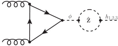
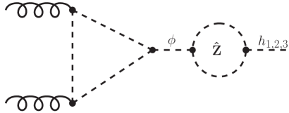
(a)	(b)

Figure 1: Feynman diagrams for the LO cross section with (a) quark and (b) squark contributions.

In this section we discuss the calculation of the gluon-fusion cross section with particular emphasis on the effects of complex parameters. We first focus on individual ingredients and then combine them in Section 4. For this purpose our notation closely follows Ref. [21]. At leading order (LO) the gluon-fusion cross section is known since a long time [69]. In addition to the quark-induced contributions, the squark-induced contributions to the gluon-fusion process are also of relevance in supersymmetric extensions of the SM, even though they are suppressed by inverse powers of the supersymmetric particle masses if those masses are heavy. Subsequently we present our calculation of the LO cross section for the case of the MSSM with complex parameters for the three physical Higgs bosons $h_{a},a\in\{1,2,3\}$. Differences with respect to the calculation in the MSSM with real parameters are induced through

• $\hat{\mathrm{\bf{Z}}}$ factors, which relate the amplitude for an external on-shell Higgs $h_{a}$ (in the mass eigenstate basis) to the amplitudes of both the $\mathcal{CP}$-even lowest-order states $h$ and $H$ and the $\mathcal{CP}$-odd state $A$, see Section 2.4.

• Non-vanishing couplings of squarks $g^{A}_{\tilde{f}ii}$ to the pseudoscalar component $A$.

• Different left- and right-handed quark couplings $g^{\phi}_{q_{L}}$ and $g^{\phi}_{q_{R}}$ with $\phi\in\{h,H,A\}$, see Section 2.1.

3.1 Lowest-order cross section

The LO production cross section of the mass eigenstates $h_{a}$ can be written as follows

$$\sigma_{\text{{LO}{}}}(pp\to h_{a})=\sigma_{0}^{h_{a}}\tau_{h_{a}}\mathcal{L}^{gg}(\tau_{h_{a}})\quad\text{with}\quad\mathcal{L}^{gg}(\tau)=\int_{\tau}^{1}\frac{dx}{x}g(x)g(\tau/x)\,,$$ (24)

where $\tau_{h_{a}}=m_{h_{a}}^{2}/s$. The hadronic squared centre-of-mass energy is denoted by $s$, and the gluon-gluon luminosity by $\mathcal{L}^{gg}$. Therein, the partonic LO cross section for $gg\to h_{a}$ is given by

$$\sigma_{0}^{h_{a}}=\frac{G_{F}\alpha_{s}^{2}(\mu_{R})}{288\sqrt{\pi}} \left[\left|\mathcal{A}^{h_{a},\mathrm{e}}\right|^{2}+\left|\mathcal{A}^{h_{a},\mathrm{o}}\right|^{2}\right]$$ (25)

with $$\mathcal{A}^{h_{a},\mathrm{e}}=\hat{\mathrm{\bf{Z}}}_{ah}\mathcal{A}_{+}^{h}+\hat{\mathrm{\bf{Z}}}_{aH}\mathcal{A}_{+}^{H}+\hat{\mathrm{\bf{Z}}}_{aA}\mathcal{A}_{-}^{A}$$

and $$\mathcal{A}^{h_{a},\mathrm{o}}=\hat{\mathrm{\bf{Z}}}_{ah}\mathcal{A}_{-}^{h}+\hat{\mathrm{\bf{Z}}}_{aH}\mathcal{A}_{-}^{H}+\hat{\mathrm{\bf{Z}}}_{aA}\mathcal{A}_{+}^{A}\,,$$

where $G_{F}$ denotes Fermi’s constant, and $\hat{\mathrm{\bf{Z}}}_{a\phi}$ are the elements of the $\hat{\mathrm{\bf{Z}}}$ factor matrix. $\mu_{\text{R}}$ is the renormalisation scale, which at LO only enters through the scale dependence of the strong coupling constant $\alpha_{s}$. We denote the cross section $pp\to h_{a}$, which involves one-loop diagrams in the production process $pp\to\phi$, as “LO cross section” despite the fact that it contains higher-order effects through the application of the $\hat{\mathrm{\bf{Z}}}$ factors (Fig. 1). We note that in the effective field theory approach of heavy quark and SUSY masses, where the gluon-gluon-Higgs interaction is condensed into a single vertex, the amplitudes of the first term in Eq. (25) can be identified with a contribution that stems from $\mathcal{L}\supset G^{\mu\nu}G_{\mu\nu}\phi$ with the gluon field strength $G^{\mu\nu}$. The amplitudes of the second term stem from $\mathcal{L}\supset\tilde{G}^{\mu\nu}G_{\mu\nu}\phi$, which involves the dual of the gluon field strength tensor $\tilde{G}^{\mu\nu}$, resulting in the cross section being expressible as the sum of two non-interfering squared amplitudes. This explains the naming of the first and the second term with $\mathcal{A}^{h_{a},\mathrm{e}}$ and $\mathcal{A}^{h_{a},\mathrm{o}}$, respectively. Similarly, we can split $\sigma_{\text{{LO}{}}}$ into $\sigma_{\text{{LO}{}}}^{\mathrm{e}}$ and $\sigma_{\text{{LO}{}}}^{\mathrm{o}}$.

For the two $\mathcal{CP}$-even lowest-order mass eigenstates $\phi^{e}\in\{h,H\}$ we obtain the amplitudes

$$\mathcal{A}_{+}^{\phi^{e}}=\sum_{q\in\{t,b\}}\left(a^{\phi^{e}}_{q,+}+\tilde{a}_{q}^{\phi^{e}}\right)\,,\quad\mathcal{A}_{-}^{\phi^{e}}=\sum_{q\in\{t,b\}}a^{\phi^{e}}_{q,-}$$ (26)

with

$$a^{\phi^{e}}_{q,+} =\frac{1}{2}\left(g_{q_{L}}^{\phi^{e}}+g_{q_{R}}^{\phi^{e}}\right)\frac{3}{2}\tau_{q}^{h_{a}}\left[1+(1-\tau_{q}^{h_{a}})f(\tau_{q}^{h_{a}})\right]\,,\quad a^{\phi^{e}}_{q,-}=\frac{i}{2}\left(g_{q_{R}}^{\phi^{e}}-g_{q_{L}}^{\phi^{e}}\right)\frac{3}{2}\tau_{q}^{h_{a}}f(\tau_{q}^{h_{a}})$$

$$\tilde{a}_{q}^{\phi^{e}} =-\frac{3}{8}\tau_{q}^{h_{a}}\sum_{i=1}^{2}g^{\phi^{e}}_{\tilde{q}ii}\left[1-\tau_{\tilde{q}i}^{h_{a}}f(\tau_{\tilde{q}i}^{h_{a}})\right]\,,$$ (27)

where $g_{q_{L}}^{\phi^{e}}$ and $g_{q_{R}}^{\phi^{e}}$ are the couplings of the Higgs boson $\phi^{e}$ to the left- and right-handed quarks, respectively. They are normalised to the SM Higgs-quark couplings. $g^{\phi^{e}}_{\tilde{q}ij}$ are the couplings of the Higgs boson $\phi^{e}$ to squarks $\tilde{q}_{i}$ and $\tilde{q}_{j}$. The explicit expressions for the Higgs-squark and relative Higgs-quark couplings are listed in Appendix A. Similarly, for the $\mathcal{CP}$-odd Higgs boson $A$ we have

$$\mathcal{A}_{-}^{A}=\sum_{q\in\{t,b\}}\left(a^{A}_{q,-}+\tilde{a}_{q}^{A}\right)\,,\quad\mathcal{A}_{+}^{A}=\sum_{q\in\{t,b\}}a^{A}_{q,+}$$ (28)

with

$$a^{A}_{q,+} =\frac{1}{2}\left(g_{q_{L}}^{A}+g_{q_{R}}^{A}\right)\frac{3}{2}\tau_{q}^{h_{a}}f(\tau_{q}^{h_{a}})\,,\quad a^{A}_{q,-}=\frac{i}{2}\left(g_{q_{L}}^{A}-g_{q_{R}}^{A}\right)\frac{3}{2}\tau_{q}^{h_{a}}\left[1+(1-\tau_{q}^{h_{a}})f(\tau_{q}^{h_{a}})\right]$$

$$\tilde{a}_{q}^{A} =-\frac{3}{8}\tau_{q}^{A}\sum_{i=1}^{2}g_{\tilde{q}ii}^{A}\left[1-\tau_{\tilde{q}_{i}}^{h_{a}}f(\tau_{\tilde{q}_{i}}^{h_{a}})\right]\,.$$ (29)

Within the previous formulas we use the notation

$$\tau_{q}^{h_{a}}=\frac{4m^{2}_{q}}{m_{h_{a}}^{2}},\hskip 14.22636pt\tau_{\tilde{q}_{i}}^{h_{a}}=\frac{4m_{\tilde{q}_{i}}^{2}}{m_{h_{a}}^{2}}\,,$$ (30)

and $f(\tau)$ is given by

$$f(\tau)=\Bigg{\{}\begin{matrix}\text{arcsin}^{2}\frac{1}{\sqrt{\tau}}&\mathrm{for}\quad\tau\geq 1\\ -\frac{1}{4}\left(\log\frac{1+\sqrt{1-\tau}}{1-\sqrt{1-\tau}}-i\pi\right)^{2}&\mathrm{for}\quad\tau<1\end{matrix}\,.$$ (31)

Our result is consistent with Ref. [13], which however assumes $g_{q_{L}}^{\phi}=g_{q_{R}}^{\phi}$ (see our discussion of this issue in Section 2.1) and does not take into account the mixing among the tree-level mass eigenstates $\phi\in\{h,H,A\}$. All squark contributions, i.e. $\tilde{a}_{q}^{\phi^{e}}$ and $\tilde{a}_{q}^{A}$, enter the first term, $\mathcal{A}^{h_{a},\mathrm{e}}$, in Eq. (25). Quark contributions to $\mathcal{A}^{h_{a},\mathrm{e}}$ which couple to the $\mathcal{CP}$-odd lowest-order mass eigenstate $A$ are proportional to the difference between the left- and right-handed quark Yukawa couplings. The same holds for the contributions to the second term $\mathcal{A}^{h_{a},\mathrm{o}}$ in Eq. (25) which couple to the $\mathcal{CP}$-even lowest-order mass eigenstates $\phi^{e}$. All these terms are therefore denoted with the subscript $\mathcal{A}_{-}$. It should be noted that the amplitudes $\mathcal{A}_{-}^{\phi_{e},A}$ only arise due to the complex nature of the Yukawa couplings, which is a consequence of the incorporation of higher-order contributions entering via $\Delta_{b}$, see Eq. (5), and our choice of working with a complex Yukawa coupling. Accordingly, the amplitudes $\mathcal{A}_{-}^{\phi_{e},A}$ are zero in the case of the MSSM with real parameters.

3.2 Higher-order contributions

Gluon fusion receives sizeable corrections at higher orders in QCD. The NLO corrections for the SM quark contributions are known for arbitrary quark masses [70, 71, 72, 73, 74, 75]. NNLO (SM-) QCD contributions were calculated in the limit of a heavy top-quark mass [76, 77, 78], similar to the recently published N³LO contributions for a $\mathcal{CP}$-even Higgs boson in an expansion around the threshold of Higgs production [79, 80, 81, 82, 83]. Finite top-quark mass effects at NNLO are known in an expansion of inverse powers of the top-quark mass [86, 87, 88, 89, 90, 91, 92, 93]. All of the previously mentioned corrections are implemented in SusHi [21, 22] and can be added in all supported models. We will later discuss in more detail for which Higgs mass ranges these corrections are applicable, which also explains why the above mentioned N³LO contributions are only employed for the $\mathcal{CP}$-even component of the light Higgs boson.

As explained above a complex Yukawa coupling is only induced for the bottom quark through the incorporation of $\Delta_{b}$ contributions. According to this approach, for the top-quark Yukawa coupling $g_{t}^{\phi}$ left- and right handed components are identical also in the MSSM with complex parameters. Therefore we can directly adapt the known higher-order QCD corrections to the top-quark loop contribution for the MSSM with complex parameters. They are incorporated in the extension SusHiMi, see Section 4. For the incorporation of the bottom-quark contribution at NLO (SM-) QCD, on the other hand, we have to rely on the simplified version of the $\Delta_{b}$ corrections to the bottom-Yukawa coupling as specified in Eq. (7). Electroweak two-loop corrections as discussed in Refs. [94, 95, 96] can be added as well. We take into account the contributions mediated by light quarks, which can be reweighted to the MSSM with complex parameters. We follow Ref. [97] and define the correction factor

$$\delta_{\text{EW}}^{\text{lf}}=\frac{\alpha_{\text{EM}}}{\pi}\frac{2\text{Re}\left(\mathcal{A}^{h_{a},\mathrm{e}}\mathcal{A}^{h_{a},\text{EW}*}\right)}{|\mathcal{A}^{{h_{a}},\mathrm{e}}|^{2}}\,,$$ (32)

where $\mathcal{A}^{h_{a},\mathrm{e}}$, which has been given in Eq. (25), denotes the $\mathcal{CP}$-even part of the LO amplitude including quark and squark contributions. Accordingly, this electroweak correction factor is only applied to the $\mathcal{CP}$-even component of the LO and NLO cross section, see Section 4. The electroweak amplitude is given by [96]

$$\mathcal{A}^{h_{a},\text{EW}}=-\frac{3}{8}\frac{x_{W}}{s_{W}^{2}} \left[\frac{2}{c_{W}^{4}}\left(\frac{5}{4}-\frac{7}{3}s_{W}^{2}+\frac{22}{9}s_{W}^{4}\right)A_{1}[x_{Z}]+4A_{1}[x_{W}]\right]$$ (33)

$$\cdot\left(-\hat{\mathrm{\bf{Z}}}_{ah}\sin\alpha\cos\beta+\hat{\mathrm{\bf{Z}}}_{aH}\cos\alpha\sin\beta\right)\,,$$

with the abbreviation

$$\begin{split}x_{V}=\frac{1}{m_{h_{a}}^{2}}\left(M_{V}-i\frac{\Gamma_{V}}{2}\right)^{2}\,,\qquad V\in\{W,Z\}\,.\end{split}$$ (34)

In Eq. (32) $\alpha_{\text{EM}}$ denotes the electro-magnetic coupling, and $s_{W}\equiv\sin\theta_{W}=(1-c_{W}^{2})^{1/2}=(1-M_{W}^{2}/M_{Z}^{2})^{1/2}$ is the sine of the weak mixing angle. $M_{V}$ and $\Gamma_{V}$ are the mass and the width of the heavy gauge bosons $V\in\{W,Z\}$, and the function $A_{1}[x]$ can be found in Ref. [96].

In the MSSM with real parameters analytical NLO virtual contributions involving squarks, quarks and gluinos are either known in the limit of a vanishing Higgs mass [98, 99, 100, 101] or in an expansion of heavy SUSY masses [102, 103, 104]. Even NNLO corrections of stop-induced contributions to gluon fusion are known [108, 109]; SusHi can approximate these NNLO stop effects [110] in the $\mathcal{CP}$-conserving MSSM. We neglect those contributions in our analysis for the MSSM with complex parameters.

At NLO in the MSSM with complex parameters, supersymmetric contributions are present both in virtual and real corrections. The real corrections show a similar behaviour as observed for the LO cross section, i.e. the squark induced contributions of $\mathcal{CP}$-odd components proportional to $g_{\tilde{q}ii}^{A}$ are added as a complex component to the $\mathcal{CP}$-even couplings. Since beyond LO we employ the simplified version of the $\Delta_{b}$ resummation according to Eq. (7), the higher-order quark contributions, both real and virtual, are of the same structure as in the $\mathcal{CP}$-conserving MSSM. The NLO virtual contributions as described in the previous paragraph are however not easily adjustable to the MSSM with complex parameters. We therefore interpolate the NLO virtual contributions between phases $0$ and $\pi$ of the various MSSM parameters using a cosine interpolation, see Refs. [111, 112]. This interpolation makes use of on-shell stop- and sbottom-quark masses defined at phases $0$ and $\pi$. Thus, within the interpolated result we have to ensure the correct subtraction of the NLO contributions that have already been taken into account through $\Delta_{b}$ effects in the bottom-quark Yukawa coupling. This is done by expanding the $\Delta_{b}$ correction to next-to-leading order in the subtraction term. For a certain value of the phase $\phi_{z}$ of a complex parameter $z$, the virtual NLO amplitude $\mathcal{A}_{\mathrm{{NLO}}{}}^{\phi}(\phi_{z})$ can be approximated using

$$\mathcal{A}_{\mathrm{{NLO}}{}}^{\phi}(\phi_{z})=\frac{1+\cos\phi_{z}}{2}\mathcal{A}_{\mathrm{{NLO}}{}}^{\phi}(0)+\frac{1-\cos\phi_{z}}{2}\mathcal{A}_{\mathrm{{NLO}}{}}^{\phi}(\pi)$$ (35)

for each of the lowest-order mass eigenstates $\phi\in\{h,H,A\}$. Here $\mathcal{A}_{\mathrm{{NLO}}{}}^{\phi}(0)$ is the analytical result for the MSSM with real parameters, and $\mathcal{A}_{\mathrm{{NLO}}{}}^{\phi}(\pi)$ is the analytical result with $z\rightarrow-z$. Using the factors $\cos\phi_{z}$ ensures a smooth interpolation such that the known results for a vanishing phase are recovered. Whereas a dependence on the phases of $A_{q}$ and $\mu$ is already apparent in the lowest-order diagrams of $gg\to\phi$, the phase of $M_{3}$ only enters through the NLO virtual corrections. Besides the $\Delta_{b}$ contributions, where the full phase dependence is incorporated, the treatment of the phase of $M_{3}$ therefore relies on the performed interpolation. While the implemented routines for the MSSM with real parameters are expressed in terms of the gluino mass, they can also be used for a negative soft-breaking parameter $M_{3}$, such that we can obtain interpolated results for a complex-valued parameter $M_{3}$. We note that the NLO virtual amplitudes with a negative $M_{3}$ are identical to the virtual amplitudes for positive $M_{3}$ with opposite signs of the parameters $A_{t},A_{b}$ and $\mu$. This can be understood from the structure of the NLO diagrams involving the squark–quark–gluino couplings. It should however be noted in this context that due to the generation of Higgs-squark couplings $g_{\tilde{q}ii}^{A}$ for non-vanishing phases a new class of NLO virtual diagrams arises which is not present in the MSSM with real parameters. Since the interpolation is based on the result for the MSSM with real parameters as input for the predictions at the phases 0 and $\pi$, the additional set of diagrams may not be adequately approximated in this way.

Despite this fact, we expect that the interpolation of the virtual two-loop contributions involving squarks and gluinos to the gluon-fusion amplitude provides a reasonable approximation, for the following reasons (we discuss the theoretical uncertainty associated with the interpolation in Section 6 and assign a conservative estimate of the uncertainty in our numerical analysis). We focus here on the gluon fusion amplitude without $\hat{\mathrm{\bf{Z}}}$ factors, since in the $\hat{\mathrm{\bf{Z}}}$ factors the full phase dependence is incorporated without approximations. Gluino contributions are generally suppressed for gluino masses that are sufficiently heavy to be in accordance with the present bounds from LHC searches, while gluon-exchange contributions do not add an additional phase dependence compared to the dependence on the phases of $A_{q}$ and $\mu$ in the LO cross section, which is fully taken into account. The dependence of the NLO amplitude on the phases of $A_{q}$ and $\mu$ is therefore expected to follow a similar pattern as the LO amplitude, which is also what we find in the application of the interpolation method.

One can also compare the higher-order corrections to the gluon-fusion process with the ones to the Higgs boson masses and $\hat{\mathrm{\bf{Z}}}$ factors. In fact, a similar interpolation was probed in the prediction for Higgs boson masses in the MSSM with complex parameters, see e.g. Refs. [28, 30, 112, 113], where the phase dependence of sub-leading two-loop contributions beyond ${\cal O}(\alpha_{t}\alpha_{s})$ were approximated with an interpolation before the full phase dependence of the corresponding two-loop corrections at ${\cal O}(\alpha_{t}^{2})$ was calculated [31, 32]. Generally good agreement was found between the full result and the approximation [31, 32]. In order to investigate the interpolation of the phase of $M_{3}$ that is associated with the gluino we performed a similar check concerning the phase dependence of two-loop squark and gluino loop contributions. We numerically compared the full result for the Higgs mass prediction at this order from FeynHiggs with an approximation where the phases at the two-loop level are interpolated. Despite the fact that also for the Higgs mass calculation new diagrams proportional to $g_{\tilde{q}ii}^{A}$ arise away from phases $0$ and $\pi$, the phase dependence of the interpolated results generically follows the behaviour of the full results very well.

Based on the NLO amplitude that has been obtained as described above, we can construct the NLO cross sections $\sigma_{\text{{NLO}{}}}^{\mathrm{e}}$ and $\sigma_{\text{{NLO}{}}}^{\mathrm{o}}$ individually, following Ref. [21], by defining the NLO correction factors $C^{\mathrm{e}}$ and $C^{\mathrm{o}}$:

$$C^{\mathrm{e/o}}=2\text{Re}\left[\frac{\mathcal{A}_{\text{{NLO}}}^{h_{a},\mathrm{e/o}}}{\mathcal{A}^{h_{a},\mathrm{e/o}}}\right]+\pi^{2}+\beta_{0}\log\left(\frac{\mu_{\text{R}}^{2}}{\mu_{\text{F}}^{2}}\right)\,.$$ (36)

The amplitudes are given by $\mathcal{A}_{\text{{NLO}}}^{h_{a},\mathrm{e}}=\hat{\mathrm{\bf{Z}}}_{ah}\mathcal{A}_{\text{{NLO}}}^{h}+\hat{\mathrm{\bf{Z}}}_{aH}\mathcal{A}_{\text{{NLO}}}^{H}$ and $\mathcal{A}_{\text{{NLO}}}^{h_{a},\mathrm{o}}=\hat{\mathrm{\bf{Z}}}_{aA}\mathcal{A}_{\text{{NLO}}}^{A}$, $\mu_{\text{F}}$ denotes the factorisation scale, and $\beta_{0}=11/2-n_{f}/3$ with $n_{f}=5$. Note that the LO amplitudes $\mathcal{A}^{h_{a},\mathrm{e/o}}$ entering Eq. (36) are taken in the limit of large stop and sbottom masses, see Ref. [21]. The correction factors enter the NLO cross section as follows

$$\sigma_{\text{{NLO}{}}}^{\mathrm{e/o}}(pp\to h_{a}+X)=\sigma_{0}^{h_{a},\mathrm{e/o}}\tau_{h_{a}}\mathcal{L}^{gg}(\tau_{h_{a}})\left[1+C^{\mathrm{e/o}}\frac{\alpha_{s}}{\pi}\right]+\Delta\sigma_{gg}^{\mathrm{e/o}}+\Delta\sigma_{gq}^{\mathrm{e/o}}+\Delta\sigma_{q\bar{q}}^{\mathrm{e/o}}\,.$$ (37)

The terms $\Delta\sigma$ denote the real corrections, which are not fully displayed here. We emphasise again that at NLO we work with Eq. (7), such that in the real corrections the only new ingredients are Higgs-squark couplings $g_{\tilde{q}ii}^{A}$, which are added to the $\mathcal{CP}$-even components $\Delta\sigma^{\mathrm{e}}$. The real corrections can be split in $\Delta\sigma^{\mathrm{e}}$ and $\Delta\sigma^{\mathrm{o}}$ since no interference terms arise.

4 The program SusHi and the extension SusHiMi

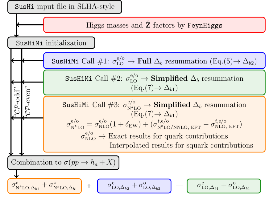
Figure 2: Pictorial view of the gluon-fusion cross section calculation.

SusHi is a numerical FORTRAN code [21, 22] which combines analytical results for the calculation of Higgs boson cross sections through gluon fusion and heavy-quark annihilation in models beyond the Standard Model up to the highest known orders in perturbation theory. However, the current release does not allow for $\mathcal{CP}$ violation in the Higgs sector. Following our discussion in Section 3 we present the calculation of Higgs boson production in the context of the MSSM with complex parameters, which we included in an extension of SusHi named SusHiMi. For this purpose we proceed along the lines of Fig. 2 and calculate the Higgs boson production cross section through gluon fusion as follows: SusHiMi calls SusHi twice and in these two calls performs a “$\mathcal{CP}$-even” calculation for $\sigma_{\text{{NLO}{}}}^{\mathrm{e}}$ and a “$\mathcal{CP}$-odd” calculation for $\sigma_{\text{{NLO}{}}}^{\mathrm{o}}$ according to Eq. (37). Thus, the total gluon-fusion cross section is the sum of the two parts

$$\sigma_{\text{{N${}^{k}$LO}}}(pp\to h_{a}+X)=\sigma_{\text{{N${}^{k}$LO}}}^{\mathrm{e}}(pp\to h_{a}+X)+\sigma_{\text{{N${}^{k}$LO}}}^{\mathrm{o}}(pp\to h_{a}+X)\,.$$ (38)

We obtain the result beyond LO QCD through

$$\sigma^{\mathrm{e}}_{\text{{N${}^{k}$LO}}}=\sigma_{\text{{NLO}{}}}^{\mathrm{e}}(1+\delta_{\mathrm{EW}}^{\mathrm{lf}})+\left(\sigma_{\text{{N${}^{k}$LO}, \text{{EFT}{}}}}^{t,\mathrm{e}}-\sigma_{\text{{NLO}{}, \text{{EFT}{}}}}^{t,\mathrm{e}}\right)$$ (39)

$$\sigma^{\mathrm{o}}_{\text{{N${}^{k}$LO}}}=\sigma_{\text{{NLO}{}}}^{\mathrm{o}}+\left(\sigma_{\text{{N${}^{k}$LO}, \text{{EFT}{}}}}^{t,\mathrm{o}}-\sigma_{\text{{NLO}{}, \text{{EFT}{}}}}^{t,\mathrm{o}}\right)\,,$$ (40)

whereas $\sigma^{\mathrm{e/o}}_{\text{{LO}{}}}$ was specified in Section 3, and $k\in\{1,2,3\}$. The $\mathcal{CP}$-odd component $\sigma_{\text{{N${}^{k}$LO}, \text{{EFT}{}}}}^{t,\mathrm{o}}$ is only implemented up to $k=2$ (see below). In the previous formulas $\sigma_{\text{{NLO}{}}}^{\mathrm{e/o}}$ are the NLO cross sections including real contributions and the interpolated NLO virtual corrections as discussed in Section 3. They employ the simplified $\Delta_{b}$ resummation according to Eq. (7), named $\Delta_{b1}$. $\sigma_{\text{{N${}^{k}$LO}, \text{{EFT}{}}}}^{t,\mathrm{e}}$ and $\sigma_{\text{{N${}^{k}$LO}, \text{{EFT}{}}}}^{t,\mathrm{o}}$ are cross sections including the top-quark contribution only. They are based on a $K$-factor calculated in the EFT approach of an infinitely heavy top-quark obtained for a SM Higgs boson $H$ and a pseudoscalar $A$ (in a 2HDM with $\tan\beta=1$) with mass $m_{h_{a}}$, respectively. This $K$-factor is subsequently reweighted with the exact LO cross section. For this purpose the employed LO cross sections $\sigma_{\text{{LO}}}^{t,\mathrm{e}}$ and $\sigma_{\text{{LO}}}^{t,\mathrm{o}}$ are again evaluated as discussed in Section 3 with full $\hat{\mathrm{\bf{Z}}}$ factors, but include only the top-quark contribution. They are multiplied with the $K$-factors in $\sigma_{\text{{N${}^{k}$LO}, \text{{EFT}{}}}}^{t,\mathrm{e}}$ and $\sigma_{\text{{N${}^{k}$LO}, \text{{EFT}{}}}}^{t,\mathrm{o}}$, respectively. Due to their small numerical impact in $\sigma_{\text{{N${}^{k}$LO}, \text{{EFT}{}}}}^{t,\mathrm{e/o}}$ we do not take into account top-quark mass effects beyond NLO even though they are implemented in SusHi. An alternative approach, which is not discussed in this paper but can be implemented in SusHiMi, is to include the relative couplings $g_{t}^{\phi}$ and the $\hat{\mathrm{\bf{Z}}}$ factors into the complex-valued Wilson coefficients of the EFT directly.

As already mentioned N³LO QCD corrections are only taken into account for the $\mathcal{CP}$-even component of the light Higgs boson, which allows us to match the precision of the light Higgs boson cross section in the SM employed in up-to-date predictions. This is motivated by the fact that the light Higgs boson that is identified with the observed signal at $125\,\text{GeV}$ is usually assumed to have a dominant $\mathcal{CP}$-even component, which is also the case in the scenarios which are considered in our numerical discussion. For the $\mathcal{CP}$-odd component of the light Higgs and the heavy Higgs bosons we employ the NNLO corrections for the top-quark induced contributions to gluon fusion in the effective theory of a heavy top-quark, i.e. we do not take into account top-quark mass effects beyond NLO, but only factor out the LO QCD cross sections $\sigma_{\text{{LO}}}^{t,\mathrm{e}}$ and $\sigma_{\text{{LO}}}^{t,\mathrm{o}}$. The strategy to employ the EFT result at NNLO beyond the top-quark mass threshold can be justified from the comparison of NLO corrections, which are known in the EFT approach and exactly with full quark-mass dependence and agree also beyond the top-quark mass threshold. On the other hand, the N³LO QCD corrections that were obtained for the top-quark contribution are only known in the EFT approach and for an expansion around the threshold of Higgs production at $x=m_{h_{a}}^{2}/s\to 1$, which we can take into account up to $\mathcal{O}(1-x)^{16}$. Since the combination of the EFT approach and the threshold expansion becomes questionable above the top-quark mass threshold, we apply N³LO QCD corrections only for the $\mathcal{CP}$-even component of the light Higgs boson and thus match the precision of the SM prediction. The electroweak correction factor $\delta_{\mathrm{EW}}^{\mathrm{lf}}$ multiplied in the “$\mathcal{CP}$-even” run is obtained from Eq. (32).

As shown in Fig. 2 we call SusHiMi three times in order to take into account the different possibilities of the resummation of $\tan\beta$ enhanced sbottom effects in the LO QCD contributions. We add the results as follows

$$\sigma(pp\to h_{a}+X)=\sigma_{\text{{N${}^{k}$LO}}}^{\Delta_{b1}}+\sigma_{\text{{LO}{}}}^{\Delta_{b2}}-\sigma_{\text{{LO}{}}}^{\Delta_{b1}}\,,$$ (41)

where in the N^kLO QCD cross section following Eq. (38) the simplified resummation according to Eq. (7) is employed, indicated through the index $\Delta_{b1}$. We add and subtract the LO QCD cross section using the full resummation according to Eq. (5), named $\Delta_{b2}$, and the simplified resummation, respectively. As we will demonstrate the differences between the two versions of resummation are small, which can partially be understood from a possible rephasing of complex Yukawa couplings by a redefinition of all (s)quark fields (see the discussion in Section 2.1).

SusHi also allows one to obtain differential cross sections as a function of the transverse momentum or the (pseudo-)rapidity of the Higgs boson. These effects can be studied also in the MSSM with complex parameters. In the case of non-vanishing transverse momentum, which is only possible through additional radiation, i.e. real corrections, the precision for massive quark contributions in extended Higgs sectors is currently limited to the LO prediction [114, 115]. The predictions of the $p_{T}$ distributions in SusHiMi have been obtained from the LO contributions with arbitrary complex parameters, and in contrast to the total cross sections are therefore not affected by additional interpolation uncertainties from higher orders in comparison to the case of the MSSM with real parameters.

Higgs production through bottom-quark annihilation is calculated in SusHi for a SM Higgs boson at NNLO QCD. In the employed five-flavour scheme, where the bottom quarks are understood as partons, the result equals the cross section of a pseudoscalar $A$ (in a 2HDM with $\tan\beta=1$). For the production of the Higgs boson $h_{a}$ in the MSSM with complex parameters, as implemented in SusHiMi, the results for the SM Higgs boson are reweighted to the MSSM with $|\hat{\mathrm{\bf{Z}}}_{ah}g_{b}^{h}+\hat{\mathrm{\bf{Z}}}_{aH}g_{b}^{H}|^{2}+|\hat{\mathrm{\bf{Z}}}_{aA}g_{b}^{A}|^{2}$, which includes $\tan\beta$-enhanced squark effects through $\Delta_{b}$ according to Eq. (7). This procedure equals the application of a $K$-factor on the full LO cross section including $\hat{\mathrm{\bf{Z}}}$ factors. In case of non-equal left- and right-handed couplings $g_{bL}$ and $g_{bR}$ due to the application of the full resummation in Eq. (5), the SM cross section has to be multiplied with

$$|\hat{\mathrm{\bf{Z}}}_{ah}(g_{bL}^{h}+g_{bR}^{h})+\hat{\mathrm{\bf{Z}}}_{aH}(g_{bL}^{H}+g_{bR}^{H})+i\hat{\mathrm{\bf{Z}}}_{aA}(g_{bL}^{A}-g_{bR}^{A})|^{2}$$

$$+|i\hat{\mathrm{\bf{Z}}}_{ah}(g_{bR}^{h}-g_{bL}^{h})+i\hat{\mathrm{\bf{Z}}}_{aH}(g_{bR}^{H}-g_{bL}^{H})+\hat{\mathrm{\bf{Z}}}_{aA}(g_{bL}^{A}+g_{bR}^{A})|^{2}\,.$$ (42)

Though, due to the similarity of both approaches we only discuss Higgs production through bottom-quark annihilation with simplified $\Delta_{b}$ resummation.

5 Numerical results

For our numerical analysis we slightly modify two standard MSSM scenarios introduced in Ref. [116], namely the $m_{h}^{\mathrm{mod}+}$ and the light-stop scenario. The scenarios have been chosen for illustration, featuring relatively large squark and gluino contributions to the gluon fusion process. The corresponding effects will be relevant in our discussion of the associated theoretical uncertainties.

The light-stop inspired scenario that we use for our numerical analysis is defined as follows

$$M_{1}=340\,\text{GeV},\quad M_{2}=\mu=400\,\text{GeV},\quad M_{3}=1.5\,\text{TeV}$$

$$X_{t}=X_{b}=X_{\tau}=1.0\,\text{TeV},\quad A_{q}=A_{l}=0$$ (43)

$$\tilde{m}_{Q_{2}}=\tilde{m}_{L}=1\,\text{TeV},\quad\tilde{m}_{Q_{3}}=0.5\,\text{TeV}\,,$$

where the modified values of $M_{1}$ and $M_{2}$ have been chosen to avoid direct bounds from stop searches obtained in LHC Run I (assuming $R$-parity conservation). For the $m_{h}^{\mathrm{mod}+}$-inspired scenario we choose for vanishing phases of the complex parameters:

$$M_{1}=250\,\text{GeV},\quad M_{2}=500\,\text{GeV},\quad M_{3}=1.5\,\text{TeV}$$

$$X_{t}=X_{b}=X_{\tau}=1.5\,\text{TeV},\quad A_{q}=A_{l}=0$$ (44)

$$\mu=\tilde{m}_{Q}=\tilde{m}_{L}=1\,\text{TeV}\,.$$

We use for the SM parameters the values $m_{t}^{\textrm{OS}}=173.20$ GeV, $m_{b}^{\overline{\textrm{MS}}}(m_{b})=4.16\,$GeV, $m_{b}^{\textrm{OS}}=4.75\,$GeV and $\alpha_{s}(M_{Z})=0.119$. The depicted on-shell bottom-quark mass is used as internal mass for propagators and for the bottom-quark Yukawa coupling in the gluon-fusion process. The depicted value of $\alpha_{s}$ is only used for the evaluations of FeynHiggs, for the cross sections the value of $\alpha_{s}$ associated with the employed PDF set is taken. We employ the MMHT2014 PDF sets at LO, NLO and NNLO QCD [118]. The central choice for the renormalisation and factorisation scales $\mu_{\text{R}}^{0}$ and $\mu_{\text{F}}^{0}$, respectively, is $(\mu_{\text{R}}^{0},\mu_{\text{F}}^{0})=(m_{h_{a}}/2,m_{h_{a}}/2)$ for gluon fusion and $(\mu_{\text{R}}^{0},\mu_{\text{F}}^{0})=(m_{h_{a}},m_{h_{a}}/4)$ for bottom-quark annihilation. More details are described in Section 6.

Whereas for the $m_{h}^{\mathrm{mod}+}$-inspired scenario we pick heavy Higgs bosons through $m_{H^{\pm}}=900$ GeV with $\tan\beta=10$ and $40$ for the study of $\Delta_{b}$ effects, we choose $m_{H^{\pm}}=500$ GeV with $\tan\beta=16$ for the light-stop inspired scenario. A detailed discussion of squark effects for the Higgs boson cross sections in the light-stop scenario can also be found in Ref. [119]. For the chosen parameter point the squark effects are sizeable, both for the light Higgs boson and in particular also for the heavy $\mathcal{CP}$-even Higgs boson, where they reduce the gluon-fusion cross section by about $\sim 90$%. The Higgs boson masses and the $\hat{\mathrm{\bf{Z}}}$ factors are obtained from FeynHiggs 2.11.2. The cross sections are evaluated with SusHiMi, which is based on the latest release of SusHi, version 1.6.1. We will mostly focus on the gluon-fusion cross section and present the bottom-quark annihilation cross section only for the scenario with $\tan\beta=40$.

For the parameter points associated with the mentioned scenarios in the MSSM with real parameters we vary the phases of $A_{t}=|A_{t}|e^{i\phi_{A_{t}}}$ and $M_{3}=m_{\tilde{g}}e^{i\phi_{M_{3}}}$ leaving the absolute values constant in order to address various aspects in the phenomenology of Higgs boson production. The phases of $A_{b}$ and $\mu$ do not introduce new phenomenological features, and we do not display results for the variation of those phases. A variation of the phase of $X_{t}$ leads to very similar cross sections for all Higgs bosons as observed for the variation of the phase of $A_{t}$. This can be understood from the fact that we choose not too large values of $\mu$ and $\tan\beta\geq 10$, and so $X_{t}\approx A_{t}$. Note that the stop masses are constant as a function of the phase of $X_{t}$, if the absolute value of $X_{t}$ is fixed. Before we proceed we want to briefly discuss experimental constraints on the phases: The most restrictive constraints on the phases arise from bounds on the electric dipole moments (EDMs) of the electron and the neutron, see Refs. [120, 121, 122] and references therein. EDMs from heavy quarks [123, 124] and the deuteron [125] also have an impact. MSSM contributions to these EDMs already contribute at the one-loop level and primarily involve the first two generations of sleptons and squarks. Thus, EDMs lead to severe constraints on the phases of $A_{q}$ for $q\in\{u,d,s,c\}$ and $A_{l}$ for $l\in\{e,\mu\}$. Using the convention that the phase of the wino soft-breaking mass $M_{2}$ is rotated away, one finds tight constraints on the phase of $\mu$ [126]. On the other hand constraints on the phases of the third-generation trilinear couplings are significantly weaker. We refer the reader to Ref. [127] for a review. While recent constraints from EDMs [128] taking into account two-loop contributions [129] have the potential to rule out the largest values of the phase of $A_{t}$, there is still significant room for variation of the phases of $A_{t}$ and $M_{3}$. We therefore display the full range of the phases of $A_{t}$ and $M_{3}$ in our considered scenarios without explicitly imposing EDM constraints, following the common approach in benchmark scenarios for Higgs phenomenology (see e.g. Ref. [130] for a recent discussion). It should be noted in this context that in particular the variation of $A_{t}$ affects the value of the stop masses. Additionally, the Higgs boson masses are a function of the phases of the complex parameters. The impact is particularly pronounced for the mass of the light Higgs boson. In order to factor out the impact of phase space effects, we normalise the prediction for the cross section of the light Higgs boson in the MSSM to the cross section of a SM Higgs boson with identical mass as the light Higgs mass eigenstate $m_{h_{1}}$. In case of the heavy Higgs bosons for which the phase space effects are much less severe, we stick to the inclusive cross sections without such a normalisation. The predicted value for the Higgs boson mass $m_{h_{1}}$ deviates from $125$ GeV by up to a few GeV in our illustrative studies. Deviations from the experimental value in this ballpark are still commensurate with the remaining theoretical uncertainties from unknown higher-order corrections of current state-of-the-art calculations of the light Higgs boson mass in the MSSM [6].

Subsequently we discuss three aspects: We start with a discussion of squark effects for the Higgs boson production cross sections. They are of relevance both for the heavy Higgs bosons and the light Higgs boson. Secondly, we focus on the admixture of the two heavy Higgs bosons (described through $\hat{\mathrm{\bf{Z}}}$ factors) and its effect on production cross sections. Lastly we discuss $\Delta_{b}$ corrections in the context of the $m_{h}^{\mathrm{mod}+}$-inspired scenario with large $\tan\beta$, for which the bottom-quark annihilation process for the heavy Higgs bosons is relevant as well.

Note that given the large admixture of the two heavy Higgs bosons in the MSSM with complex parameters, interference effects in the full processes of production and decay can be large. However, we restrict our discussion in the present paper to Higgs boson production. The results for the cross sections obtained in our paper can be employed in a generalised narrow-width approximation as described in Ref. [7] in order to incorporate interference effects. We will address this issue elsewhere.

The prediction for Higgs boson cross sections is affected by various theoretical uncertainties, which we discuss in detail in Section 6. In order to demonstrate the improvement in precision through the inclusion of higher-order corrections, all subsequent figures which show the LO cross section and our best prediction cross section according to Eq. (38) include renormalisation and factorisation scale uncertainties. The procedure for obtaining these scale uncertainties is outlined in Section 6.

5.1 Squark contributions in the light-stop inspired scenario

We start with a discussion of squark effects to the Higgs boson cross section $\sigma(gg\to h_{i})$ for all three Higgs bosons $h_{i}$ in the context of the light-stop inspired scenario with $m_{H^{\pm}}=500$ GeV and $\tan\beta=16$. The variation of the light Higgs boson mass $m_{h_{1}}$ as well as the stop masses is depicted in Fig. 3 (a) as a function of $\phi_{A_{t}}$. The light Higgs mass in this scenario may appear to be too light to be compatible with the signal observed at the LHC, however we regard it as sufficiently close in view of the facts that our discussion should demonstrate phenomenological effects only and that on the other hand there are still sizeable theoretical uncertainties in the MSSM prediction for the light Higgs boson mass. The lightest stop mass has its minimum at around $308$ GeV. For the heavy Higgs bosons with masses between $492$ and $494$ GeV, which are not shown in the figures, the NLO squark-gluino contributions [102, 103, 104] which assume heavy squarks and gluinos are thus well applicable. The variation of the heavy Higgs boson masses as a function of the phases of $\phi_{A_{t}}$ and $\phi_{M_{3}}$ turns out to be small, namely within $0.6$ GeV. Due to the strong admixture of the left- and right-handed stops through a large value of $A_{t}$, also a phase dependence of the stop masses is observed. We checked that if we instead choose a phase for $X_{t}$ keeping $|X_{t}|$ constant, we obtain constant stop masses if the phase of $X_{t}$ is varied.

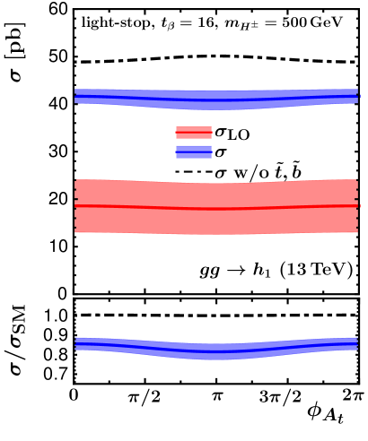
(a)	(b)

Figure 3: (a) Mass of $h_{1}$ and stop masses in GeV as a function of $\phi_{A_{t}}$; (b) LO (red) and best prediction for the gluon-fusion cross section (blue) for the light Higgs $h_{1}$ in pb as a function of $\phi_{A_{t}}$. The results are shown for the light-stop inspired scenario as specified in Eq. (43). The black, dot-dashed curve depicts the best prediction cross section without squark contributions (except through $\hat{\mathrm{\bf{Z}}}$ factors). The depicted uncertainties are scale uncertainties. In the lower panel we normalise to the cross section of a SM Higgs boson with the same mass $m_{h_{1}}$.

Fig. 3 (b) shows the production cross section through gluon fusion for the light Higgs boson $h_{1}$. The black, dot-dashed curve depicts the cross section with top-quark and bottom-quark contributions and electroweak corrections in the production amplitudes only, i.e. in the formulas of Section 4 we omit all squark contributions which enter either directly or through $\Delta_{b}$. Note however that squark contributions are always part of the $\hat{\mathrm{\bf{Z}}}$ factors. Due to the decoupling with large values of $m_{H^{\pm}}$ in our scenarios the light Higgs $h_{1}$ has mostly SM-like couplings to quarks and gauge bosons. Thus, thanks to the inclusion of N³LO QCD contributions for the top-quark induced contribution, our prediction of the gluon fusion cross section omitting the squark contributions (black, dot-dashed curve in Fig. 3 (b)) is very close to the one for the SM Higgs boson with the same mass as provided by the LHC Higgs Cross Section Working Group [6, 131]. The inclusion of squark contributions explicitly and through $\Delta_{b}$ resummation lowers the gluon-fusion cross section by about $20$%, as can be inferred from the blue, solid curve, which is shown together with its renormalisation and factorisation scale uncertainty, see Section 6. For completeness we also show the LO cross section calculated according to Eq. (24) including squark effects as the red curve. It is apparent that the scale uncertainties are significantly reduced from LO QCD to our best prediction cross section calculated according to Eq. (38). Fig. 3 (b) also includes the cross section for $h_{1}$ normalised to the cross section of a SM Higgs boson with the same mass. Here the $\sim 20$% reduction due to squark effects is apparent once again, whereas the quark-induced cross section shows the well-known decoupling behaviour. Not shown in the figures are the following effects, which we state here for completeness: The variation of $\phi_{M_{3}}$ leads to a very similar picture, even though the light Higgs mass variation is not as pronounced and the stop masses are unaffected. Moreover, in the comparison of the simplified and the full resummation of $\Delta_{b}$ contributions in the LO gluon-fusion cross section of $h_{1}$ we observe a well-known behaviour, namely the simplified resummation of Eq. (7) does not yield a decoupled bottom-quark Yukawa coupling, whereas the full resummation of Eq. (5) does.

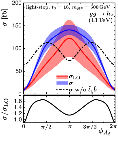
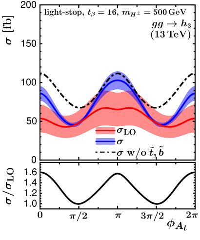
(a)	(b)

Figure 4: LO (red) and best prediction for the gluon-fusion cross section (blue) for (a) $h_{2}$ and (b) $h_{3}$ in fb as a function of $\phi_{A_{t}}$. The results are shown for the light-stop inspired scenario as specified in Eq. (43). The black, dot-dashed curve depicts the best prediction cross section without squark contributions (except through $\hat{\mathrm{\bf{Z}}}$ factors). The depicted uncertainties are scale uncertainties. In the lower panel we show the $K$-factor $\sigma/\sigma_{{LO}}$.

In Fig. 4 (a) and (b) we show the gluon-fusion cross sections of the heavy Higgs bosons $h_{2}$ and $h_{3}$, respectively, as a function of $\phi_{A_{t}}$. The colour coding is identical to Fig. 3 except for the fact that we show the $K$-factor of our best prediction for the cross section with respect to the LO cross section, $\sigma/\sigma_{{LO}{}}$, rather than a cross section normalised to the SM Higgs boson cross section. In fact, the heavy Higgs masses change only slightly as a function of the phase $\phi_{A_{t}}$, and therefore the associated phase space effect is small. For vanishing phase $\phi_{A_{t}}=0$ it is known that squark effects are huge and reduce the cross section by $\sim 89$% ($h_{2}$) and $\sim 22$% ($h_{3}$) [119]. These squark effects are strongly dependent on the phase $\phi_{A_{t}}$ and induce a large positive correction at phase $\phi_{A_{t}}=\pi$ in case of $h_{2}$. For $h_{3}$ the effects are not as pronounced, but still sizeable. The $K$-factor for both processes $gg\to h_{2}$ and $gg\to h_{3}$ remains within $[1,1.6]$, i.e. higher-order corrections mainly follow the phase dependence of the LO cross section. The dependence of the $K$-factor on $\phi_{A_{t}}$ follows the black, dot-dashed curve, which shows the cross section with quark contributions only. The significant dependence of the cross section where only quark contributions are included on the phase $\phi_{A_{t}}$ is induced by the admixture of the two Higgs bosons through $\hat{\mathrm{\bf{Z}}}$ factors. We will discuss this feature in detail for the $m_{h}^{\mathrm{mod}+}$-inspired scenario in Section 5.2.

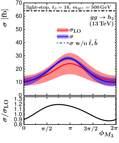
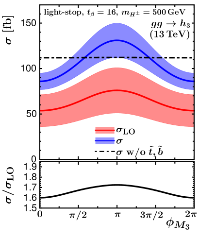
(a)	(b)

Figure 5: LO (red) and best prediction for the gluon-fusion cross section (blue) for (a) $h_{2}$ and (b) $h_{3}$ in fb as a function of $\phi_{M_{3}}$. The results are shown for the light-stop inspired scenario as specified in Eq. (43). The black, dot-dashed curve depicts the best prediction cross section without squark contributions (except through $\hat{\mathrm{\bf{Z}}}$ factors). The depicted uncertainties are scale uncertainties. In the lower panel we show the $K$-factor $\sigma/\sigma_{{LO}}$.

The phase dependence on $\phi_{M_{3}}$ is less pronounced. We show the corresponding cross sections for the two heavy Higgs bosons $h_{2}$ and $h_{3}$ in Fig. 5. As in previous figures we observe a significant reduction in the scale dependence from LO QCD to our best prediction for the cross section. The inclusion of squark and gluino contributions through the $\hat{\mathrm{\bf{Z}}}$ factors and through $\Delta_{b}$ induces a dependence on the gluino phase already for the LO cross section. The almost flat black dot-dashed curves show the cross section with quark contributions only, and any variation with $\phi_{M_{3}}$ is an effect of the $\hat{\mathrm{\bf{Z}}}$ factors, which in this case is negligible since $\phi_{M_{3}}$ only enters at the two-loop level. The $K$-factor, which takes into account our interpolated NLO virtual corrections, only shows a relatively mild dependence on the phase. We will discuss the interpolation uncertainty for this scenario in Section 6, since we obtain the largest relative interpolation uncertainty in the cross section variation with phases for the interpolation of the gluino phase $\phi_{M_{3}}$.

5.2 Admixture of Higgs bosons in the $m_{h}^{\mathrm{mod}+}$-inspired scenario

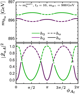
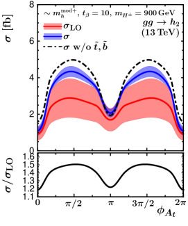
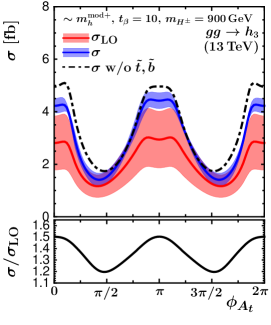
(a)	(b)	(c)

Figure 6: (a) Masses of $h_{2}$ and $h_{3}$ in GeV as well as $\mathcal{CP}$-odd character $|\hat{\mathrm{\bf{Z}}}_{aA}|^{2}$ as a function of $\phi_{A_{t}}$ in the $m_{h}^{\mathrm{mod}+}$-inspired scenario with $\tan\beta=10$. The solid and dashed curves depict regions in $\phi_{A_{t}}$ where $h_{2}$ and $h_{3}$ are predominantly $\mathcal{CP}$-even ($h_{e}$) or odd ($h_{o}$), respectively, corresponding to $|\hat{\mathrm{\bf{Z}}}_{aA}|^{2}$ being below or above $0.5$ as shown in the lower panel. (b,c) LO (red) and best prediction for the gluon-fusion cross section (blue) for (b) $h_{2}$ and (c) $h_{3}$ in fb as a function of $\phi_{A_{t}}$ in the same scenario. The black, dot-dashed curve depicts the best prediction for the cross section without squark contributions (except through $\hat{\mathrm{\bf{Z}}}$ factors). In the lower panel we show the $K$-factor $\sigma/\sigma_{{LO}}$. The depicted uncertainties are scale uncertainties.

In this subsection we discuss the $m_{h}^{\mathrm{mod}+}$-inspired scenario with $\tan\beta=10$ and $m_{H^{\pm}}=900$ GeV. Since the squark masses are at the TeV level in this scenario, the numerical effect of the squark loops in the gluon fusion vertex contributions is rather small for the production cross section of the light Higgs boson $h_{1}$. We do not discuss the results for $h_{1}$ in this section. The results for the two heavy Higgs bosons are displayed in Fig. 6. The effects from squark loops are at the level of about $\pm 20$% in this case. The considered scenario is typical for the decoupling region of supersymmetric theories, where a light SM-like Higgs boson (that is interpreted as the signal observed at about 125 GeV) is accompanied by additional heavy Higgs bosons that are nearly mass-degenerate. In the general case where the possibility of $\mathcal{CP}$-violating interactions is taken into account, there can be a large mixing between the $\mathcal{CP}$-even and $\mathcal{CP}$-odd neutral Higgs states. This feature is clearly visible in Fig. 6. The dependence on the phase $\phi_{A_{t}}$ is seen to be closely correlated to the mixing character of the two neutral heavy Higgs bosons.

Fig. 6 (a) depicts the masses of the two heavy Higgs bosons $h_{2}$ and $h_{3}$ as a function of $\phi_{A_{t}}$ together with the $\mathcal{CP}$-odd character of $h_{2}$ and $h_{3}$, being defined as $|\hat{\mathrm{\bf{Z}}}_{aA}|^{2}$. For illustration here and in the following we call the mass eigenstates $h_{2}$ and $h_{3}$ either $h_{e}$ or $h_{o}$, depending on their mixing character: if $|\hat{\mathrm{\bf{Z}}}_{aA}|^{2}\gtrsim 1/2$ the mass eigenstate $h_{a}$ is called $h_{o}$, otherwise it is called $h_{e}$. It can be seen in Fig. 6 (b) and (c) that the behaviour of the cross sections as a function of $\phi_{A_{t}}$ closely follows the variation in the $\mathcal{CP}$-even and $\mathcal{CP}$-odd character of the Higgs states. A similar effect was already apparent in the top- and bottom-quark induced cross sections depicted in the light-stop inspired scenario, see Fig. 4, however there the effects of squark contributions are dominant. Also in this case the scale uncertainty of our best prediction for the cross section is significantly reduced in comparison to the uncertainty for the prediction in LO QCD. The variation of the $K$-factors between about 1.2 and 1.5 with the phase $\phi_{A_{t}}$ also follows the modification of the mixing character of the two neutral heavy Higgs bosons.

Since the two heavy Higgs bosons are nearly mass degenerate, it may not be possible in such a case to experimentally resolve the two Higgs bosons as separate signals. Rather than the individual cross sections times their respective branching ratios, the experimentally measurable quantity then consists of the sum of the cross sections of the two Higgs states times their respective branching ratios together with the interference contribution involving the two Higgs states. The latter can be particularly important if the mass difference between the two Higgs states is smaller than the sum of their total widths [7]. While we defer the incorporation of such interference effects into the prediction for the production and decay process to a forthcoming publication, one can already infer from the plots of Fig. 6 (b) and (c) that in the overall contribution there will be sizeable cancellations between the phase dependencies of the separate contributions.

5.3 $\Delta_{b}$ corrections in the $m_{h}^{\mathrm{mod}+}$-inspired scenario

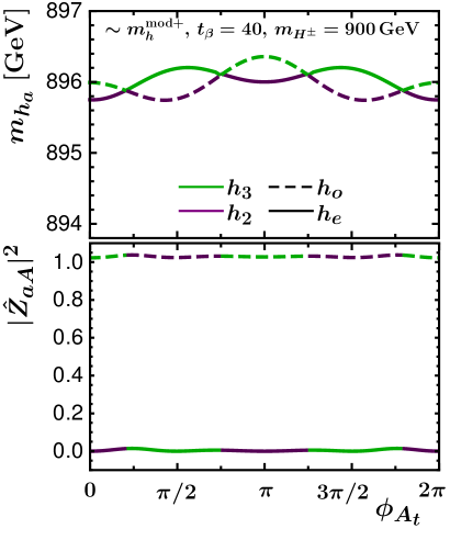
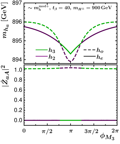
(a)	(b)

Figure 7: Masses of $h_{2}$ and $h_{3}$ in GeV and $\mathcal{CP}$-odd character as a function of (a) $\phi_{A_{t}}$ and (b) $\phi_{M_{3}}$ in the $m_{h}^{\mathrm{mod}+}$-inspired scenario with $\tan\beta=40$. As in Fig. 6 (a), the solid and dashed curves refer to $h_{e}$ and $h_{o}$, respectively.

We finally discuss the impact of $\Delta_{b}$ effects, which we investigate for the two heavy Higgs bosons in the $m_{h}^{\mathrm{mod}+}$-inspired scenario with $\tan\beta=40$. In this scenario the admixture between the two heavy Higgs bosons is again sizeable both as a function of $\phi_{A_{t}}$ and as a function of $\phi_{M_{3}}$. This even leads to mass crossings as seen in Fig. 7. It is therefore convenient to discuss the results in terms of the predominantly $\mathcal{CP}$-even mass eigenstate $h_{e}$ and the predominantly $\mathcal{CP}$-odd mass eigenstate $h_{o}$, as defined in Section 5.2, as for those states a smooth behaviour of the cross section as function of the phases is obtained. The masses of the two heavy Higgs bosons and their $\mathcal{CP}$-character (defining $h_{o}$ and $h_{e}$) are shown in Fig. 7 as a function of $\phi_{A_{t}}$ and $\phi_{M_{3}}$. One can see that the states $h_{2}$ and $h_{3}$ drastically change their $\mathcal{CP}$ character upon variation of the phases $\phi_{A_{t}}$ and $\phi_{M_{3}}$, while on the other hand the state $h_{e}$ is almost purely $\mathcal{CP}$-even and $h_{o}$ is almost purely $\mathcal{CP}$-odd for the whole range of phase values. It should be kept in mind in this context that $|\hat{\mathrm{\bf{Z}}}_{aA}|^{2}$ arises from a non-unitary matrix and can therefore have values above 1. For vanishing phases the mass eigenstate $h_{2}$ corresponds to $h_{e}$ and $h_{3}$ to $h_{o}$.

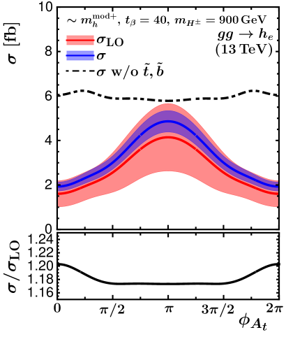
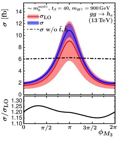
(a)	(b)

Figure 8: LO (red) and best prediction gluon-fusion cross section (blue) for $h_{e}$ in fb as a function of (a) $\phi_{A_{t}}$ and (b) $\phi_{M_{3}}$ in the $m_{h}^{\mathrm{mod}+}$-inspired scenario with $\tan\beta=40$. The black dot-dashed curves depict the best prediction cross section without squark contributions (except through $\hat{\mathrm{\bf{Z}}}$ factors). In the lower panel we show the $K$-factor $\sigma/\sigma_{{LO}}$. The depicted uncertainties are scale uncertainties.

In the following we show results for the predominantly $\mathcal{CP}$-even mass eigenstate $h_{e}$. The observations for $h_{o}$ are very similar and are not shown here, we will only add comments where appropriate. In Fig. 8 we show the gluon-fusion cross section as a function of the phases $\phi_{A_{t}}$ and $\phi_{M_{3}}$. In both cases the behaviour for the full prediction, including the squark contributions, is dominated by $\Delta_{b}$ corrections. For vanishing phases those corrections significantly reduce the cross sections compared to the case where only quark contributions are taken into account. For phase values around $\pi$, however, the $\Delta_{b}$ corrections can also give rise to a significant enhancement of the cross section. In particular, for $\phi_{M_{3}}$ the quantity $\Delta_{b}$ changes sign between $\phi_{M_{3}}=0$ and $\phi_{M_{3}}=\pi$, such that the bottom-Yukawa coupling is suppressed for small values of $\phi_{M_{3}}$ and enhanced for $\phi_{M_{3}}$ values close to $\pi$ as a consequence of the resummation of the $\Delta_{b}$ corrections. The reduction of the scale uncertainties from LO QCD to our best prediction for the cross section is similar as in the previous plots. The $K$-factors in the lower panel show that the dependence of the NLO cross sections on the phases $\phi_{A_{t}}$ and $\phi_{M_{3}}$ follows a similar trend as the LO cross section. In the plot on the right, the asymmetric $K$-factor dependence on $\phi_{M_{3}}$ is related to the direct dependence of $\Delta_{b}$ on the phase $\phi_{M_{3}}$.

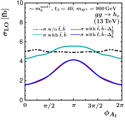
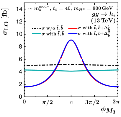
(a)	(b)

Figure 9: Effect of $\Delta_{b}$ contributions on the LO cross sections of $h_{e}$ as a function of (a) $\phi_{A_{t}}$ and (b) $\phi_{M_{3}}$ in the $m_{h}^{\mathrm{mod}+}$-inspired scenario with $\tan\beta=40$. The black dot-dashed curves depict the prediction without squark contributions (except through $\hat{\mathrm{\bf{Z}}}$ factors), while the cyan lines correspond to the prediction where the squark loop contributions at the one-loop level are included. In the red (blue) curves furthermore the simplified (full) resummation of the $\Delta_{b}$ contributions is included.

In Fig. 9 we separately analyse the squark contributions for the LO cross section, i.e. the prediction omitting the squark loop contributions (black dot-dashed curves) is compared with the ones where first the pure LO squark contributions are added (depicted in cyan), and then the resummation of the $\Delta_{b}$ contributions to the bottom-quark Yukawa coupling is taken into account. For the latter both the results for the full ($\Delta_{b2}$, blue) and the simplified ($\Delta_{b1}$, red) resummation are shown. While the the pure LO squark contributions are seen to have a moderate effect, it can be seen that the incorporation of the resummation of the $\Delta_{b}$ contribution leads to a significant enhancement of the squark loop effects. We furthermore confirm that for the heavy neutral Higgs bosons considered here the simplified resummation approximates the full resummation of the $\Delta_{b}$ contribution very well. The curves corresponding to $\Delta_{b2}$ and $\Delta_{b1}$ hardly differ from each other both for the variation of $\phi_{A_{t}}$ and $\phi_{M_{3}}$. As before all curves include the same $\hat{\mathrm{\bf{Z}}}$ factors obtained from FeynHiggs. The results for $h_{o}$, which are not shown here, are qualitatively very similar. The LO squark contributions are less relevant for the $h_{o}$ cross section, since those contributions are absent in the MSSM with real parameters. We also note that the curves for $h_{o}$ follow a similar behaviour as the ones for $h_{e}$, which implies that there are no large cancellations expected in the sum of the cross sections for the two heavy Higgs bosons times their respective branching ratios. Thus, the phases entering $\Delta_{b}$ could potentially lead to observable effects in the production of the two heavy Higgs bosons even if the two states cannot be experimentally resolved as separate signals.

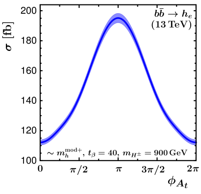
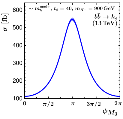
(a)	(b)

Figure 10: Bottom-quark annihilation cross section for $h_{e}$ in fb as a function of (a) $\phi_{A_{t}}$ and (b) $\phi_{M_{3}}$ in the $m_{h}^{\mathrm{mod}+}$-inspired scenario with $\tan\beta=40$. The depicted uncertainties are scale uncertainties.

Having discussed the three different sources for $\mathcal{CP}$-violating effects relevant for Higgs boson production through gluon fusion in the MSSM — squark loop contributions, admixtures through $\hat{\mathrm{\bf{Z}}}$ factors and resummation of $\Delta_{b}$ contributions — for completeness we also briefly discuss the bottom-quark annihilation cross section for the $m_{h}^{\mathrm{mod}+}$-inspired scenario with $\tan\beta=40$. The corresponding cross section is shown in Fig. 10 as a function of $\phi_{A_{t}}$ and $\phi_{M_{3}}$. For such a large value of $\tan\beta$ this cross section exceeds the gluon-fusion cross section by far. It shows a very significant dependence on the phases $\phi_{A_{t}}$ and $\phi_{M_{3}}$, which is mainly induced by the $\Delta_{b}$ contribution.

6 Remaining theoretical uncertainties

In the previous section we analysed our cross section predictions regarding $\mathcal{CP}$-violating effects entering via squark loop contributions, $\hat{\mathrm{\bf{Z}}}$ factors and $\Delta_{b}$ contributions. Therein, we included renormalisation and factorisation scale uncertainties, which as expected are reduced upon inclusion of higher-order corrections. However, the cross section predictions are also affected by other relevant theoretical uncertainties, which we want to discuss in detail in this section.

Some of the theoretical uncertainties of cross sections in the MSSM with complex parameters are very similar to the ones in the MSSM with real parameters as discussed in Ref. [119]. Therefore, we can directly transfer the discussion of PDF$+\alpha_{s}$ uncertainties as well as the uncertainty associated with the renormalisation prescription for the bottom-quark Yukawa coupling from the case of the MSSM with real parameters:

• PDF$+\alpha_{s}$ uncertainties: The fitted parton distribution functions (PDF) and the associated value of $\alpha_{s}$ induce an uncertainty in the prediction of the gluon-fusion cross section and, in particular, also the bottom-quark annihilation cross section. In our calculation we employ the MMHT2014 PDF sets at LO, NLO and NNLO [118], which can be used for both gluon fusion and bottom-quark annihilation. In Refs. [119, 24] it was observed that despite the effects of squarks in supersymmetric models, the PDF$+\alpha_{s}$ uncertainties are mostly a function of the Higgs boson mass $m_{h_{a}}$. We will therefore not discuss them in more detail, since – similar to the prescription for MSSM Higgs boson cross sections by the LHC Higgs Cross Section Working Group [6] – relative uncertainties can be taken over from tabulated relative uncertainties obtained for the SM Higgs boson or a pseudoscalar (in a 2HDM with $\tan\beta=1$) as a function of its mass. For Higgs masses in the range between $50$ GeV and $1$ TeV the typical size of PDF$+\alpha_{s}$ uncertainties for gluon fusion is $\pm(3-5)$% following the prescription of Ref. [132]. They increase up to $\pm 10$% for Higgs masses up to $2$ TeV. For bottom-quark annihilation they are in the range $\pm(3-8)$% for Higgs masses between $50$ GeV and $1$ TeV and up to $\pm 16$% for Higgs masses below $2$ TeV.

• Renormalisation of the bottom-quark mass and definition of the bottom Yukawa coupling: In our calculation the bottom-quark mass is renormalised on-shell, and the bottom-Yukawa coupling is obtained from the bottom-quark mass as described in Section 2.1. The renormalisation of the bottom-quark mass and the freedom in the definition of the bottom-Yukawa coupling are known to have a sizeable numerical impact on the cross section predictions. This is in particular the case for large values of $\tan\beta$ where the bottom-Yukawa coupling of the heavy Higgs bosons is significantly enhanced and the top-quark Yukawa coupling is suppressed. On the other hand, in these regions of parameter space bottom-quark annihilation is the dominant process, for which there is less ambiguity regarding an appropriate choice for the renormalisation scale. The described uncertainties in the MSSM with complex parameters are analogous to the case of real parameters. We therefore refer to the discussion in Ref. [119] and references therein for further details.

We neglect approximate NNLO stop-quark contributions and accordingly the uncertainty associated with the approximation of the involved Wilson coefficients, which was discussed in Ref. [119]. The impact of the NNLO stop-quark contributions for the case of the MSSM with real parameters can be compared with our estimate for the renormalisation and factorisation scale uncertainty of our calculation. As an example, the NNLO stop-quark contributions lower the inclusive cross section for the light Higgs boson by about $2$ pb for zero phases in the light-stop inspired scenario, which is at the lower edge of the scale uncertainty depicted in Fig. 3 (b). Other uncertainties discussed in Ref. [119] are renormalisation and factorisation scale uncertainties and an uncertainty related to higher-order contributions to $\Delta_{b}$. Moreover, we add another uncertainty related to the performed interpolation of supersymmetric NLO QCD contributions. We discuss in the following our estimates for the three previously mentioned uncertainties:

• We obtain the renormalisation and factorisation scale uncertainty as follows: The central scale choice is $(\mu_{\text{R}}^{0},\mu_{\text{F}}^{0})=(m_{h_{a}}/2,m_{h_{a}}/2)$ for gluon fusion and $(\mu_{\text{R}}^{0},\mu_{\text{F}}^{0})=(m_{h_{a}},m_{h_{a}}/4)$ for bottom-quark annihilation. We obtain the scale uncertainty by taking the maximal deviation from the central scale choice $\Delta\sigma$ obtained from the additional scale choices $(\mu_{\text{R}},\mu_{\text{F}})\in\{{(2\mu_{\text{R}}^{0},2\mu_{\text{F}}^{0}),(2\mu_{\text{R}}^{0},\mu_{\text{F}}^{0}),(\mu_{\text{R}}^{0},2\mu_{\text{F}}^{0}),(\mu_{\text{R}}^{0},\mu_{\text{F}}^{0}/2),(\mu_{\text{R}}^{0}/2,\mu_{\text{F}}^{0}),(\mu_{\text{R}}^{0}/2,\mu_{\text{F}}^{0}/2)\}}$. We perform this procedure individually for all three cross sections in Eq. (41) and then obtain the overall absolute uncertainty through

  $$\Delta\sigma^{\mathrm{scale}}=\sqrt{\left(\Delta\sigma_{\text{{N${}^{k}$LO}}}^{\Delta_{b1}}\right)^{2}+\left(\Delta\sigma_{\text{{LO}{}}}^{\Delta_{b2}}-\Delta\sigma_{\text{{LO}{}}}^{\Delta_{b1}}\right)^{2}}\,,$$ (45)

  where we assume the two LO cross sections to be fully correlated. The uncertainty bands that we have displayed in the plots shown above correspond to the cross section range covered by $\sigma\pm\Delta\sigma^{\mathrm{scale}}$.

• In order to display the propagation of an uncertainty arising from higher-order contributions to $\Delta_{b}$ to our cross section calculation, we vary the value of $\Delta_{b}$ obtained from FeynHiggs by $\pm 10\%$. This variation by $\pm 10\%$ roughly corresponds to the effect of a variation of the renormalisation scales, see the discussion in Ref. [119]. We label the obtained uncertainty as $\Delta\sigma^{\mathrm{resum}}$ and assign an uncertainty band of $\sigma\pm\Delta\sigma^{\mathrm{resum}}$.

• The employed interpolation for the two-loop virtual squark-gluino contributions following Eq. (35) leads to a further uncertainty. A conservative estimate for it can be obtained as follows: We determine the cross section $\sigma(\phi_{z})$ following Eq. (38) not only for the correct phase $\phi_{z}$ in Eq. (35), but also leave the phase within Eq. (35) constant, i.e. fixed to $0$ and $\pi$. We call the obtained cross sections $\sigma(0)$ and $\sigma(\pi)$. For each value of $\phi_{z}$ we take the difference $\Delta\sigma^{\mathrm{int}}=\sin^{2}(\phi_{z})|\sigma(0)-\sigma(\pi)|/2$. It is reweighted with $\sin^{2}(\phi_{z})$, since we know that our result is correct at phases $0$ and $\pi$. The obtained uncertainty band is given by $\sigma\pm\Delta\sigma^{\mathrm{int}}$.

In the following we display the effects of the estimated uncertainties for certain scenarios, where we choose the displayed scenarios and the displayed cross sections such that the effect of the uncertainties is largest. While the scale uncertainties were included in all previous figures for the LO prediction as well as for our best prediction already, we will discuss the interpolation uncertainty for the light-stop inspired scenario with $\tan\beta=16$ and the resummation uncertainty for the $m_{h}^{\mathrm{mod}+}$-inspired scenario with $\tan\beta=40$.

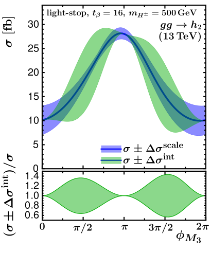
(a)	(b)

Figure 11: Renormalisation and factorisation scale uncertainties $\Delta\sigma^{\mathrm{scale}}$ (blue) and interpolation uncertainties $\Delta\sigma^{\mathrm{int}}$ (green) for the gluon-fusion cross section of (a) $h_{2}$ and (b) $h_{3}$ as a function of $\phi_{M_{3}}$ in the light-stop inspired scenario. In the lower panel the upper and lower edge of the band of the cross section prediction with the assigned interpolation uncertainty is normalised to the cross section without this uncertainty.

Fig. 11 shows the renormalisation and factorisation scale uncertainties $\Delta\sigma^{\mathrm{scale}}$ as before and in addition the above described interpolation uncertainty $\Delta\sigma^{\mathrm{int}}$, which in case of the variation of $\phi_{M_{3}}$ can be substantial. As can be seen in Fig. 11, the interpolation uncertainty obtained from our conservative estimate can in this scenario even exceed the scale uncertainty for the gluon-fusion cross section of $h_{2}$. It should be noted that this is an extreme case, while the interpolation uncertainty, which is an NLO effect related to the squark and gluino loop contributions, remains small for the other previously described scenarios (which we do not show here explicitly). This is simply a consequence of the fact that the relative impact of the squark and gluino contributions in the other scenarios is much smaller than in the light-stop inspired scenario. The interpolation uncertainty for the gluon-fusion cross section of $h_{3}$ in Fig. 11 is much less pronounced than for $h_{2}$, since as discussed above the squark loop corrections are significantly smaller in this case and would vanish if $h_{3}$ were a pure $\mathcal{CP}$-odd state. The behaviour in the lower panels of Fig. 11 displays the fact that by construction the assigned interpolation uncertainty vanishes for the phases 0 and $\pi$, where the interpolated result in the MSSM with complex parameters merges the known result of the MSSM with real parameters. For the variation of $\phi_{A_{t}}$ the LO cross section incorporating squark contributions already includes the dominant effect on the cross section, such that the uncertainty due to the interpolated NLO contributions is also less pronounced than in case of the variation of $\phi_{M_{3}}$.

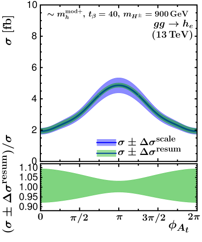
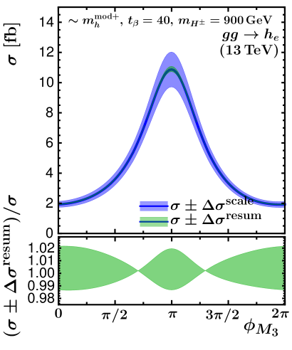
(a)	(b)

Figure 12: Renormalisation and factorisation scale uncertainties $\Delta\sigma^{\mathrm{scale}}$ (blue) and resummation uncertainties $\Delta\sigma^{\mathrm{resum}}$ (green) for the gluon-fusion cross section of $h_{e}$ as a function of (a) $\phi_{A_{t}}$ and (b) $\phi_{M_{3}}$ in the $m_{h}^{\mathrm{mod}+}$-inspired scenario for $\tan\beta=40$. In the lower panel the upper and lower edge of the band of the cross section prediction with the assigned resummation uncertainty is normalised to the cross section without this uncertainty.

The described $\Delta_{b}$ uncertainties are depicted in Fig. 12. Since $\Delta_{b}$ crosses $0$ as a function of $\phi_{M_{3}}$ twice, the uncertainty that we have associated to it according to the prescription discussed above also vanishes there, as can be seen in the lower panel of Fig. 12(b). Even for the large value of $\tan\beta$ chosen here the assigned $\Delta_{b}$ uncertainty of $\pm 10\%$ is much smaller than the scale uncertainty of the displayed cross sections. Despite the different behaviour with the phases $\phi_{A_{t}}$ and $\phi_{M_{3}}$ displayed in the lower panel of Fig. 12 the qualitative effect of the resummation uncertainties on the Higgs boson production cross sections is nevertheless rather similar. The latter is also true for the bottom-quark annihilation cross section, which is not depicted here. The resummation uncertainties are of most relevance for large values of $\tan\beta$, where the cross section of bottom-quark annihilation exceeds the gluon-fusion cross section.

7 Conclusions

In this paper we have presented theoretical predictions for inclusive cross sections for neutral Higgs boson production via gluon fusion and bottom-quark annihilation in the MSSM with complex parameters, and demonstrated the relevance of the $\mathcal{CP}$-violating phases on these cross sections.

The cross section predictions for the gluon-fusion process at leading-order are based on an explicit calculation taking into account the dependence on all complex parameters in the MSSM, and the complete form of the analytical formulae for the general $\mathcal{CP}$-violating case including Higgs mixing has been presented in the literature for the first time. The wave function normalisation factors arising from the $(3\times 3)$-mixing of the lowest-order mass eigenstates of the Higgs bosons $\{h,H,A\}$ into the loop-corrected mass eigenstates $\{h_{1},h_{2},h_{3}\}$ have been described with full propagator corrections using the self-energies of the neutral Higgs bosons as provided by FeynHiggs. Furthermore, the LO predictions for the gluon-fusion process in the MSSM with complex parameters deviate from those of the MSSM with real parameters due to non-zero couplings of the squarks to the pseudoscalar $A$ and potentially different left- and right-handed bottom-Yukawa couplings arising from the resummation of $\tan\beta$-enhanced sbottom contributions in $\Delta_{b}$. We have supplemented the LO computation of the cross section by higher-order contributions: using for the treatment of the higher-order corrections a simplified version of the $\Delta_{b}$ resummation we have included the full massive top- and bottom quark contributions at NLO QCD and have interpolated the NLO SUSY QCD corrections from the amplitudes in the MSSM with real parameters. We have thoroughly discussed the uncertainties involved in using such an interpolation. The interpolation uncertainty at NLO, which is most relevant in scenarios where the squarks and the gluino are relatively light in view of the present limits from the LHC searches, could be avoided if an explicit result for the squark-gluino contributions at NLO QCD in the MSSM becomes available for the general case of complex parameters. For the top-quark contribution in the effective theory of a heavy top-quark we have added NNLO QCD contributions for all Higgs bosons, and N³LO QCD contributions in an expansion around the threshold of Higgs production for the $\mathcal{CP}$-even component of the light Higgs boson $h_{1}$ to match the precision of the predictions for the SM Higgs boson. Electroweak effects, which include two-loop contributions with couplings of the heavy gauge bosons to the $\mathcal{CP}$-even component of the Higgs bosons mediated by light quarks, have been added to the $\mathcal{CP}$-even component of the gluon-fusion cross section.

The results presented in this paper are currently the state of the art for neutral Higgs production in the MSSM with complex parameters. Our calculations have been implemented in an extension of the code SusHi called SusHiMi, which is linked to FeynHiggs. SusHiMi is available upon request. Using SusHiMi, we have investigated the phenomenological effects of $\mathcal{CP}$-violating phases on the production of Higgs bosons in the MSSM with complex parameters in two slightly modified benchmark scenarios, light-stop and $m_{h}^{\text{mod+}}$. We have found in our analysis of Higgs boson production through gluon fusion that a proper description of squark and gluino loop contributions is essential. This refers both to the loop contributions to the gluon–gluon–Higgs vertex and to the corrections entering through $\Delta_{b}$. Squark and gluino loop contributions furthermore enter the wave function normalisation factors that are necessary to ensure the correct on-shell properties of the produced Higgs boson. Where squark and gluino contributions are sizeable the production cross sections show a significant dependence on the $\mathcal{CP}$-violating phases. We have discussed the remaining theoretical uncertainties in the cross section predictions taking into account renormalisation and factorisation scale uncertainties, a resummation uncertainty for $\Delta_{b}$ and an uncertainty due to the performed interpolation of NLO SUSY QCD corrections. We have furthermore briefly commented on other uncertainties that can directly be taken over from the case of the MSSM with real parameters.

A further important feature that occurs in the production processes for the two heavy states $h_{2}$ and $h_{3}$ in the general case where $\mathcal{CP}$-violating interactions are taken into account is the fact that there can be a large mixing between these often nearly mass-degenerate states. Their mixing effects are incorporated in the wave function normalisation factors for the external Higgs bosons. For a proper interpretation of experimental exclusion limits arising from MSSM Higgs searches, which so far have only been analysed in the framework of the $\mathcal{CP}$-conserving MSSM, it will be important to take into account interference effects in the full process of Higgs production and decay. Our results for the cross sections for on-shell Higgs bosons can be directly used in the context of a generalised narrow-width approximation to incorporate these interference effects. This topic will be addressed in a forthcoming publication.

Appendix A Formulas: Higgs-quark and Higgs-squark couplings

In SusHiMi the Higgs–(s)quark couplings are expressed in terms of the $\mathcal{CP}$-even and $\mathcal{CP}$-odd neutral gauge eigenstates $\phi_{g}\in\{\phi_{1}^{0},\phi_{2}^{0}\}$ and $\chi_{g}\in\{\chi_{1}^{0},\chi_{2}^{0}\}$, respectively. In order to obtain the couplings of the squarks with the lowest-order mass eigenstates $\phi\in\{h,H,A,G\}$ the gauge eigenstates are rotated using the tree-level mixing matrix $\mathcal{R}$ as depicted in the following Feynman diagrams

$$\parbox{76.82243pt}{\includegraphics[width=91.04742pt]{figures/coupq.pdf}}=\left\{\begin{matrix}i\frac{m_{q}}{v}\mathcal{R}(g_{q_{L}}^{\phi_{g}}P_{L}+g_{q_{R}}^{\phi_{g}}P_{R})\\ -\frac{m_{q}}{v}\mathcal{R}(g_{q_{L}}^{\chi_{g}}P_{L}-g_{q_{R}}^{\chi_{g}}P_{R})\end{matrix}\right.\qquad\text{and}\qquad\parbox{76.82243pt}{\includegraphics[width=91.04742pt]{figures/coupsq.pdf}}=i\frac{1}{v}\mathcal{R}g_{\tilde{q},ij}^{\phi_{g},\chi_{g}}$$ (46)

with $v=2m_{W}/g=1/\sqrt{\sqrt{2}G_{F}}$ and the tree-level mixing matrix $\mathcal{R}$ given in Eq. (11). At the amplitude level the results will then also be multiplied with the corresponding $\hat{\mathrm{\bf{Z}}}$ factor.

The couplings between the gauge eigenstates and the third generation quarks are $g_{q_{L}}=1/\cos\beta$ for $\phi_{1}^{0}$ and $\chi_{1}^{0}$ and $g_{q_{L}}=1/\sin\beta$ for $\phi_{2}^{0}$ and $\chi_{2}^{0}$. For $\Delta_{b}$ corrections we refer to Eq. (5) and Eq. (7).

The couplings between the gauge eigenstates and the third generation squarks contain terms from the squark mass diagonalisation matrix $U_{\tilde{q}}$ (see Eq. (3)) which is a unitary matrix with real diagonal elements and complex off-diagonal elements, i.e. it can be written as follows

$$U_{\tilde{q}}=\begin{pmatrix}U_{\tilde{q}11}&U_{\tilde{q}12}\\ -U_{\tilde{q}12}^{*}&U_{\tilde{q}22}\end{pmatrix}\,.$$ (47)

They are obtained with MaCoR [133, 134]. For the $\mathcal{CP}$-even state $\phi_{1}^{0}$ we have the stop couplings (using $s_{\beta}\equiv\sin{\beta}$, $c_{\beta}\equiv\cos{\beta}$, $t_{\beta}\equiv\tan{\beta},s_{W}\equiv\sin\theta_{W}$ and $c_{W}\equiv\cos\theta_{W}$):

$$g_{\tilde{t},11}^{\phi_{1}^{0}} =U_{\tilde{t}12}^{*}\left[-\frac{U_{\tilde{t}11}m_{t}\mu}{s_{\beta}}+\frac{4}{3}U_{\tilde{t}12}c_{\beta}m_{Z}^{2}s^{2}_{W}\right]-U_{\tilde{t}11}^{*}\left[\frac{U_{\tilde{t}12}m_{t}\mu^{*}}{s_{\beta}}+c_{\beta}m_{Z}^{2}U_{\tilde{t}11}\left(\frac{s^{2}_{W}}{3}-c_{W}^{2}\right)\right]$$

$$g_{\tilde{t},12}^{\phi_{1}^{0}} =U_{\tilde{t}12}^{*}\left[-\frac{U_{\tilde{t}21}m_{t}\mu}{s_{\beta}}+\frac{4}{3}U_{\tilde{t}22}c_{\beta}m_{Z}^{2}s^{2}_{W}\right]-U_{\tilde{t}11}^{*}\left[\frac{U_{\tilde{t}22}m_{t}\mu^{*}}{s_{\beta}}+c_{\beta}m_{Z}^{2}U_{\tilde{t}21}\left(\frac{s^{2}_{W}}{3}-c_{W}^{2}\right)\right]$$

$$g_{\tilde{t},21}^{\phi_{1}^{0}} =U_{\tilde{t}22}^{*}\left[-\frac{U_{\tilde{t}11}m_{t}\mu}{s_{\beta}}+\frac{4}{3}U_{\tilde{t}12}c_{\beta}m_{Z}^{2}s^{2}_{W}\right]-U_{\tilde{t}21}^{*}\left[\frac{U_{\tilde{t}12}m_{t}\mu^{*}}{s_{\beta}}+c_{\beta}m_{Z}^{2}U_{\tilde{t}11}\left(\frac{s^{2}_{W}}{3}-c_{W}^{2}\right)\right]$$

$$g_{\tilde{t},22}^{\phi_{1}^{0}} =U_{\tilde{t}22}^{*}\left[-\frac{U_{\tilde{t}21}m_{t}\mu}{s_{\beta}}+\frac{4}{3}U_{\tilde{t}22}c_{\beta}m_{Z}^{2}s^{2}_{W}\right]-U_{\tilde{t}21}^{*}\left[\frac{U_{\tilde{t}22}m_{t}\mu^{*}}{s_{\beta}}+c_{\beta}m_{Z}^{2}U_{\tilde{t}21}\left(\frac{s^{2}_{W}}{3}-c_{W}^{2}\right)\right]\,.$$ (48)

For the $\mathcal{CP}$-even state $\phi_{2}^{0}$, the couplings are:

$$g_{\tilde{t},11}^{\phi_{2}^{0}} =U_{\tilde{t}12}^{*}\left[\frac{U_{\tilde{t}11}m_{t}A_{t}^{*}}{s_{\beta}}+U_{\tilde{t}12}\left(\frac{2m^{2}_{t}}{s_{\beta}}-\frac{4}{3}s_{\beta}m_{z}^{2}s^{2}_{W}\right)\right]$$

$$+U_{\tilde{t}11}^{*}\left[\frac{U_{\tilde{t}12}m_{t}A_{t}}{s_{\beta}}+\frac{2U_{\tilde{t}11}m^{2}_{t}}{s_{\beta}}+s_{\beta}m_{Z}^{2}U_{\tilde{t}11}\left(\frac{s^{2}_{W}}{3}-c^{2}_{W}\right)\right]$$

$$g_{\tilde{t},12}^{\phi_{2}^{0}} =U_{\tilde{t}12}^{*}\left[\frac{U_{\tilde{t}21}m_{t}A_{t}^{*}}{s_{\beta}}+U_{\tilde{t}22}\left(\frac{2m^{2}_{t}}{s_{\beta}}-\frac{4}{3}s_{\beta}m_{z}^{2}s^{2}_{W}\right)\right]$$

$$+U_{\tilde{t}11}^{*}\left[\frac{U_{\tilde{t}22}m_{t}A_{t}}{s_{\beta}}+\frac{2U_{\tilde{t}21}m^{2}_{t}}{s_{\beta}}+s_{\beta}m_{Z}^{2}U_{\tilde{t}21}\left(\frac{s^{2}_{W}}{3}-c^{2}_{W}\right)\right]$$

$$g_{\tilde{t},21}^{\phi_{2}^{0}} =U_{\tilde{t}22}^{*}\left[\frac{U_{\tilde{t}11}m_{t}A_{t}^{*}}{s_{\beta}}+U_{\tilde{t}12}\left(\frac{2m^{2}_{t}}{s_{\beta}}-\frac{4}{3}s_{\beta}m_{z}^{2}s^{2}_{W}\right)\right]$$

$$+U_{\tilde{t}21}^{*}\left[\frac{U_{\tilde{t}12}m_{t}A_{t}}{s_{\beta}}+\frac{2U_{\tilde{t}11}m^{2}_{t}}{s_{\beta}}+s_{\beta}m_{Z}^{2}U_{\tilde{t}11}\left(\frac{s^{2}_{W}}{3}-c^{2}_{W}\right)\right]$$

$$g_{\tilde{t},22}^{\phi_{2}^{0}} =U_{\tilde{t}22}^{*}\left[\frac{U_{\tilde{t}21}m_{t}A_{t}^{*}}{s_{\beta}}+U_{\tilde{t}22}\left(\frac{2m^{2}_{t}}{s_{\beta}}-\frac{4}{3}s_{\beta}m_{z}^{2}s^{2}_{W}\right)\right]$$

$$+U_{\tilde{t}21}^{*}\left[\frac{U_{\tilde{t}22}m_{t}A_{t}}{s_{\beta}}+\frac{2U_{\tilde{t}21}m^{2}_{t}}{s_{\beta}}+s_{\beta}m_{Z}^{2}U_{\tilde{t}21}\left(\frac{s^{2}_{W}}{3}-c^{2}_{W}\right)\right]\,.$$ (49)

Similarly for the $\mathcal{CP}$-odd states $\chi_{1}^{0}$ and $\chi_{2}^{0}$ the stop couplings are given as:

$$g_{\tilde{t},11}^{\chi_{1}^{0}} =i\frac{m_{t}}{s_{\beta}}\left[-\mu U_{\tilde{t}12}^{*}U_{\tilde{t}11}+\mu^{*}U_{\tilde{t}11}^{*}U_{\tilde{t}12}\right] g_{\tilde{t},11}^{\chi_{2}^{0}}=i\frac{m_{t}}{s_{\beta}}\left[-A_{t}^{*}U_{\tilde{t}12}^{*}U_{\tilde{t}11}+A_{t}U_{\tilde{t}11}^{*}U_{\tilde{t}12}\right]$$

$$g_{\tilde{t},12}^{\chi_{1}^{0}} =i\frac{m_{t}}{s_{\beta}}\left[-\mu U_{\tilde{t}12}^{*}U_{\tilde{t}21}+\mu^{*}U_{\tilde{t}11}^{*}U_{\tilde{t}22}\right] g_{\tilde{t},12}^{\chi_{2}^{0}}=i\frac{m_{t}}{s_{\beta}}\left[-A_{t}^{*}U_{\tilde{t}12}^{*}U_{\tilde{t}21}+A_{t}U_{\tilde{t}11}^{*}U_{\tilde{t}22}\right]$$

$$g_{\tilde{t},21}^{\chi_{1}^{0}} =i\frac{m_{t}}{s_{\beta}}\left[-\mu U_{\tilde{t}22}^{*}U_{\tilde{t}11}+\mu^{*}U_{\tilde{t}21}^{*}U_{\tilde{t}12}\right] g_{\tilde{t},21}^{\chi_{2}^{0}}=i\frac{m_{t}}{s_{\beta}}\left[-A_{t}^{*}U_{\tilde{t}22}^{*}U_{\tilde{t}11}+A_{t}U_{\tilde{t}21}^{*}U_{\tilde{t}12}\right]$$

$$g_{\tilde{t},22}^{\chi_{1}^{0}} =i\frac{m_{t}}{s_{\beta}}\left[-\mu U_{\tilde{t}22}^{*}U_{\tilde{t}21}+\mu^{*}U_{\tilde{t}21}^{*}U_{\tilde{t}22}\right] g_{\tilde{t},22}^{\chi_{2}^{0}}=i\frac{m_{t}}{s_{\beta}}\left[-A_{t}^{*}U_{\tilde{t}22}^{*}U_{\tilde{t}21}+A_{t}U_{\tilde{t}21}^{*}U_{\tilde{t}22}\right]\,.$$ (50)

Analogously, the Higgs-sbottom couplings for the $\mathcal{CP}$-even state $\phi_{1}^{0}$ are:

$$g_{\tilde{b},11}^{\phi_{1}^{0}} =U_{\tilde{b}12}^{*}\left[\frac{U_{\tilde{b}11}A_{b}^{*}m_{b}}{c_{\beta}}+U_{\tilde{b}12}\left(\frac{2m_{b}^{2}}{c_{\beta}}-\frac{2}{3}c_{\beta}m_{Z}^{2}s_{W}^{2}\right)\right]$$

$$+U_{\tilde{b}11}^{*}\left[\frac{U_{\tilde{b}12}A_{b}m_{b}}{c_{\beta}}+\frac{2U_{\tilde{b}11}m_{b}^{2}}{c_{\beta}}-c_{\beta}m_{Z}^{2}U_{\tilde{b}11}\left(\frac{s^{2}_{W}}{3}+c_{W}^{2}\right)\right]$$

$$g_{\tilde{b},12}^{\phi_{1}^{0}} =U_{\tilde{b}12}^{*}\left[\frac{U_{\tilde{b}21}A_{b}^{*}m_{b}}{c_{\beta}}+U_{\tilde{b}22}\left(\frac{2m_{b}^{2}}{c_{\beta}}-\frac{2}{3}c_{\beta}m_{Z}^{2}s_{W}^{2}\right)\right]$$

$$+U_{\tilde{b}11}^{*}\left[\frac{U_{\tilde{b}22}A_{b}m_{b}}{c_{\beta}}+\frac{2U_{\tilde{b}21}m_{b}^{2}}{c_{\beta}}-c_{\beta}m_{Z}^{2}U_{\tilde{b}21}\left(\frac{s^{2}_{W}}{3}+c_{W}^{2}\right)\right]\,,$$

$$g_{\tilde{b},21}^{\phi_{1}^{0}} =U_{\tilde{b}22}^{*}\left[\frac{U_{\tilde{b}11}A_{b}^{*}m_{b}}{c_{\beta}}+U_{\tilde{b}12}\left(\frac{2m_{b}^{2}}{c_{\beta}}-\frac{2}{3}c_{\beta}m_{Z}^{2}s_{W}^{2}\right)\right]$$

$$+U_{\tilde{b}21}^{*}\left[\frac{U_{\tilde{b}12}A_{b}m_{b}}{c_{\beta}}+\frac{2U_{\tilde{b}11}m_{b}^{2}}{c_{\beta}}-c_{\beta}m_{Z}^{2}U_{\tilde{b}11}\left(\frac{s^{2}_{W}}{3}+c_{W}^{2}\right)\right]$$

$$g_{\tilde{b},22}^{\phi_{1}^{0}} =U_{\tilde{b}22}^{*}\left[\frac{U_{\tilde{b}21}A_{b}^{*}m_{b}}{c_{\beta}}+U_{\tilde{b}22}\left(\frac{2m_{b}^{2}}{c_{\beta}}-\frac{2}{3}c_{\beta}m_{Z}^{2}s_{W}^{2}\right)\right]$$

$$+U_{\tilde{b}21}^{*}\left[\frac{U_{\tilde{b}22}A_{b}m_{b}}{c_{\beta}}+\frac{2U_{\tilde{b}21}m_{b}^{2}}{c_{\beta}}-c_{\beta}m_{Z}^{2}U_{\tilde{b}21}\left(\frac{s^{2}_{W}}{3}+c_{W}^{2}\right)\right]\,.$$ (51)

For the $\mathcal{CP}$-even state $\phi_{0}^{2}$ they are given as:

$$g_{\tilde{b},11}^{\phi_{2}^{0}} =U_{\tilde{b}12}^{*}\left[-\frac{U_{\tilde{b}11}m_{b}\mu}{c_{\beta}}+\frac{2}{3}U_{\tilde{b}12}s_{\beta}m_{z}^{2}s_{W}^{2}\right]-U_{\tilde{b}11}^{*}\left[\frac{U_{\tilde{b}12}m_{b}\mu^{*}}{c_{\beta}}-s_{\beta}m_{Z}^{2}U_{\tilde{b}11}\left(\frac{s^{2}_{W}}{3}+c_{W}^{2}\right)\right]$$

$$g_{\tilde{b},12}^{\phi_{2}^{0}} =U_{\tilde{b}12}^{*}\left[-\frac{U_{\tilde{b}21}m_{b}\mu}{c_{\beta}}+\frac{2}{3}U_{\tilde{b}22}s_{\beta}m_{z}^{2}s_{W}^{2}\right]-U_{\tilde{b}11}^{*}\left[\frac{U_{\tilde{b}22}m_{b}\mu^{*}}{c_{\beta}}-s_{\beta}m_{Z}^{2}U_{\tilde{b}21}\left(\frac{s^{2}_{W}}{3}+c_{W}^{2}\right)\right]$$

$$g_{\tilde{b},21}^{\phi_{2}^{0}} =U_{\tilde{b}22}^{*}\left[-\frac{U_{\tilde{b}11}m_{b}\mu}{c_{\beta}}+\frac{2}{3}U_{\tilde{b}12}s_{\beta}m_{z}^{2}s_{W}^{2}\right]-U_{\tilde{b}21}^{*}\left[\frac{U_{\tilde{b}12}m_{b}\mu^{*}}{c_{\beta}}-s_{\beta}m_{Z}^{2}U_{\tilde{b}11}\left(\frac{s^{2}_{W}}{3}+c_{W}^{2}\right)\right]$$

$$g_{\tilde{b},22}^{\phi_{2}^{0}} =U_{\tilde{b}22}^{*}\left[-\frac{U_{\tilde{b}21}m_{b}\mu}{c_{\beta}}+\frac{2}{3}U_{\tilde{b}22}s_{\beta}m_{z}^{2}s_{W}^{2}\right]-U_{\tilde{b}21}^{*}\left[\frac{U_{\tilde{b}22}m_{b}\mu^{*}}{c_{\beta}}-s_{\beta}m_{Z}^{2}U_{\tilde{b}21}\left(\frac{s^{2}_{W}}{3}+c_{W}^{2}\right)\right].$$ (52)

Finally, for the $\mathcal{CP}$-odd states $\chi_{1}^{0}$ and $\chi_{2}^{0}$ the Higgs-sbottom couplings are:

$$g_{\tilde{b},11}^{\chi_{1}^{0}} =i\frac{m_{b}}{c_{\beta}}\left[-A_{b}^{*}U_{\tilde{b}12}^{*}U_{\tilde{b}11}+A_{b}U_{\tilde{b}11}^{*}U_{\tilde{b}12}\right] g_{\tilde{b},11}^{\chi_{2}^{0}}=i\frac{m_{b}}{c_{\beta}}\left[-\mu U_{\tilde{b}12}^{*}U_{\tilde{b}11}+\mu^{*}U_{\tilde{b}11}^{*}U_{\tilde{b}12}\right]$$

$$g_{\tilde{b},12}^{\chi_{1}^{0}} =i\frac{m_{b}}{c_{\beta}}\left[-A_{b}^{*}U_{\tilde{b}12}^{*}U_{\tilde{b}21}+A_{b}U_{\tilde{b}11}^{*}U_{\tilde{b}22}\right] g_{\tilde{b},12}^{\chi_{2}^{0}}=i\frac{m_{b}}{c_{\beta}}\left[-\mu U_{\tilde{b}12}^{*}U_{\tilde{b}21}+\mu^{*}U_{\tilde{b}11}^{*}U_{\tilde{b}22}\right]$$

$$g_{\tilde{b},21}^{\chi_{1}^{0}} =i\frac{m_{b}}{c_{\beta}}\left[-A_{b}^{*}U_{\tilde{b}22}^{*}U_{\tilde{b}11}+A_{b}U_{\tilde{b}21}^{*}U_{\tilde{b}12}\right] g_{\tilde{b},21}^{\chi_{2}^{0}}=i\frac{m_{b}}{c_{\beta}}\left[-\mu U_{\tilde{b}22}^{*}U_{\tilde{b}11}+\mu^{*}U_{\tilde{b}21}^{*}U_{\tilde{b}12}\right]$$

$$g_{\tilde{b},22}^{\chi_{1}^{0}} =i\frac{m_{b}}{c_{\beta}}\left[-A_{b}^{*}U_{\tilde{b}22}^{*}U_{\tilde{b}21}+A_{b}U_{\tilde{b}21}^{*}U_{\tilde{b}22}\right] g_{\tilde{b},22}^{\chi_{2}^{0}}=i\frac{m_{b}}{c_{\beta}}\left[-\mu U_{\tilde{b}22}^{*}U_{\tilde{b}21}+\mu^{*}U_{\tilde{b}21}^{*}U_{\tilde{b}22}\right]\,.$$ (53)

References

- [1] G. Aad et al. [ATLAS Collaboration], Phys. Lett. B 716 (2012) 1 [arXiv:1207.7214].
- [2] S. Chatrchyan et al. [CMS Collaboration], Phys. Lett. B 716 (2012) 30 [arXiv:1207.7235].
- [3] S. Dittmaier et al., “Handbook of LHC Higgs Cross Sections: 1. Inclusive Observables,” arXiv:1101.0593.
- [4] S. Dittmaier et al., “Handbook of LHC Higgs Cross Sections: 2. Differential Distributions,” arXiv:1201.3084.
- [5] S. Heinemeyer et al., “Handbook of LHC Higgs Cross Sections: 3. Higgs Properties,” arXiv:1307.1347.
- [6] D. de Florian et al., “Handbook of LHC Higgs Cross Sections: 4. Deciphering the Nature of the Higgs Sector,” arXiv:1610.07922.
- [7] E. Fuchs, S. Thewes and G. Weiglein, Eur. Phys. J. C 75 (2015) 254 [arXiv:1411.4652].
- [8] N. Cabibbo, Phys. Rev. Lett. 10 (1963) 531.
- [9] M. Kobayashi and T. Maskawa, Prog. Theor. Phys. 49 (1973) 652.
- [10] A. Riotto, hep-ph/9807454.
- [11] J. M. Cline, hep-ph/0609145.
- [12] S. Davidson, E. Nardi and Y. Nir, Phys. Rept. 466 (2008) 105 [arXiv:0802.2962].
- [13] A. Dedes and S. Moretti, Nucl. Phys. B 576 (2000) 29 [hep-ph/9909418].
- [14] S. Y. Choi and J. S. Lee, Phys. Rev. D 61 (2000) 115002 [hep-ph/9910557].
- [15] S. Y. Choi, K. Hagiwara and J. S. Lee, Phys. Lett. B 529 (2002) 212 [hep-ph/0110138].
- [16] M. Carena, J. R. Ellis, S. Mrenna, A. Pilaftsis and C. E. M. Wagner, Nucl. Phys. B 659 (2003) 145 [hep-ph/0211467].
- [17] A. Arhrib, D. K. Ghosh and O. C. W. Kong, Phys. Lett. B 537 (2002) 217 [hep-ph/0112039].
- [18] Q. H. Cao, D. Nomura, K. Tobe and C.-P. Yuan, Phys. Lett. B 632 (2006) 688 [hep-ph/0508311].
- [19] S. Hesselbach, S. Moretti, S. Munir and P. Poulose, Eur. Phys. J. C 54 (2008) 129 [arXiv:0706.4269].
- [20] S. Hesselbach, S. Moretti, S. Munir and P. Poulose, Phys. Rev. D 82 (2010) 074004 [arXiv:0903.0747].
- [21] R. V. Harlander, S. Liebler and H. Mantler, Comput. Phys. Commun. 184 (2013) 1605 [arXiv:1212.3249].
- [22] R. V. Harlander, S. Liebler and H. Mantler, Comput. Phys. Commun. 212 (2017) 239 [arXiv:1605.03190].
- [23] R. V. Harlander, Eur. Phys. J. C 76 (2016) no.5, 252 [arXiv:1512.04901].
- [24] S. Liebler, Eur. Phys. J. C 75 (2015) 5, 210 [arXiv:1502.07972].
- [25] S. Heinemeyer, W. Hollik and G. Weiglein, Comput. Phys. Commun. 124 (2000) 76 [hep-ph/9812320].
- [26] S. Heinemeyer, W. Hollik and G. Weiglein, Eur. Phys. J. C 9 (1999) 343 [hep-ph/9812472].
- [27] G. Degrassi, S. Heinemeyer, W. Hollik, P. Slavich and G. Weiglein, Eur. Phys. J. C 28 (2003) 133 [hep-ph/0212020].
- [28] M. Frank, T. Hahn, S. Heinemeyer, W. Hollik, H. Rzehak and G. Weiglein, JHEP 0702 (2007) 047 [hep-ph/0611326].
- [29] T. Hahn, S. Heinemeyer, W. Hollik, H. Rzehak and G. Weiglein, Phys. Rev. Lett. 112 (2014) no.14, 141801 [arXiv:1312.4937].
- [30] S. Heinemeyer, W. Hollik, H. Rzehak and G. Weiglein, Phys. Lett. B 652 (2007) 300 [arXiv:0705.0746].
- [31] W. Hollik and S. Paßehr, Phys. Lett. B 733 (2014) 144 [arXiv:1401.8275].
- [32] W. Hollik and S. Paßehr, JHEP 1410 (2014) 171 [arXiv:1409.1687].
- [33] J. S. Lee, A. Pilaftsis, M. Carena, S. Y. Choi, M. Drees, J. R. Ellis and C. E. M. Wagner, Comput. Phys. Commun. 156 (2004) 283 [hep-ph/0307377].
- [34] J. S. Lee, M. Carena, J. Ellis, A. Pilaftsis and C. E. M. Wagner, Comput. Phys. Commun. 180 (2009) 312 [arXiv:0712.2360].
- [35] K. E. Williams and G. Weiglein, Phys. Lett. B 660 (2008) 217 [arXiv:0710.5320].
- [36] A. C. Fowler and G. Weiglein, JHEP 1001 (2010) 108 [arXiv:0909.5165].
- [37] K. E. Williams, H. Rzehak and G. Weiglein, Eur. Phys. J. C 71 (2011) 1669 [arXiv:1103.1335].
- [38] E. Fuchs, DESY-THESIS-2015-037, PhD thesis 2015.
- [39] E. Fuchs and G. Weiglein, arXiv:1610.06193.
- [40] N. Kauer, Phys. Lett. B 649 (2007) 413 [hep-ph/0703077].
- [41] D. Berdine, N. Kauer and D. Rainwater, Phys. Rev. Lett. 99 (2007) 111601 [hep-ph/0703058].
- [42] C. F. Uhlemann and N. Kauer, Nucl. Phys. B 814 (2009) 195 [arXiv:0807.4112].
- [43] G. Cacciapaglia, A. Deandrea and S. De Curtis, Phys. Lett. B 682 (2009) 43 [arXiv:0906.3417].
- [44] J. Reuter, eConf C 0705302 (2007) SUS14 [arXiv:0709.0068].
- [45] A. C. Fowler, http://etheses.dur.ac.uk/449/1/Thesis_AFowler.pdf, PhD thesis 2010.
- [46] D. Barducci, A. Belyaev, J. Blamey, S. Moretti, L. Panizzi and H. Prager, JHEP 1407 (2014) 142 [arXiv:1311.3977].
- [47] A. Djouadi, P. Gambino, S. Heinemeyer, W. Hollik, C. Junger and G. Weiglein, Phys. Rev. D 57 (1998) 4179 [hep-ph/9710438].
- [48] T. Banks, Nucl. Phys. B 303 (1988) 172.
- [49] L. J. Hall, R. Rattazzi and U. Sarid, Phys. Rev. D 50 (1994) 7048 [hep-ph/9306309].
- [50] R. Hempfling, Phys. Rev. D 49 (1994) 6168.
- [51] M. S. Carena, M. Olechowski, S. Pokorski and C. E. M. Wagner, Nucl. Phys. B 426 (1994) 269 [hep-ph/9402253].
- [52] M. S. Carena, D. Garcia, U. Nierste and C. E. M. Wagner, Nucl. Phys. B 577 (2000) 88 [hep-ph/9912516].
- [53] M. Carena, D. Garcia, U. Nierste and C. E. M. Wagner, Phys. Lett. B 499 (2001) 141 [hep-ph/0010003].
- [54] J. Baglio, R. Gröber, M. Mühlleitner, D. T. Nhung, H. Rzehak, M. Spira, J. Streicher and K. Walz, Comput. Phys. Commun. 185 (2014) no.12, 3372 [arXiv:1312.4788].
- [55] M. Frank, L. Galeta, T. Hahn, S. Heinemeyer, W. Hollik, H. Rzehak and G. Weiglein, Phys. Rev. D 88 (2013) no.5, 055013 [arXiv:1306.1156].
- [56] L. Hofer, U. Nierste and D. Scherer, JHEP 0910 (2009) 081 [arXiv:0907.5408].
- [57] D. Noth and M. Spira, JHEP 1106 (2011) 084 [arXiv:1001.1935].
- [58] D. Noth and M. Spira, Phys. Rev. Lett. 101 (2008) 181801 [arXiv:0808.0087].
- [59] A. Bauer, L. Mihaila and J. Salomon, JHEP 0902 (2009) 037 [arXiv:0810.5101].
- [60] R. D. Peccei and H. R. Quinn, Phys. Rev. D 16 (1977) 1791.
- [61] R. D. Peccei and H. R. Quinn, Phys. Rev. Lett. 38 (1977) 1440.
- [62] A. Bharucha, A. Fowler, G. Moortgat-Pick and G. Weiglein, JHEP 1305 (2013) 053 [arXiv:1211.3134].
- [63] O. Brein, A. Djouadi and R. Harlander, Phys. Lett. B 579 (2004) 149 [hep-ph/0307206].
- [64] R. V. Harlander, S. Liebler and T. Zirke, JHEP 1402 (2014) 023 [arXiv:1307.8122].
- [65] P. H. Chankowski, S. Pokorski and J. Rosiek, Nucl. Phys. B 423 (1994) 437 [hep-ph/9303309].
- [66] A. Dabelstein, Nucl. Phys. B 456 (1995) 25 [hep-ph/9503443].
- [67] S. Heinemeyer, W. Hollik, J. Rosiek and G. Weiglein, Eur. Phys. J. C 19 (2001) 535 [hep-ph/0102081].
- [68] H. Lehmann, K. Symanzik and W. Zimmermann, Nuovo Cim. 1 (1955) 205.
- [69] H. M. Georgi, S. L. Glashow, M. E. Machacek and D. V. Nanopoulos, Phys. Rev. Lett. 40 (1978) 692.
- [70] A. Djouadi, M. Spira and P. M. Zerwas, Phys. Lett. B 264 (1991) 440.
- [71] S. Dawson, Nucl. Phys. B 359 (1991) 283.
- [72] M. Spira, A. Djouadi, D. Graudenz and P. M. Zerwas, Nucl. Phys. B 453 (1995) 17 [hep-ph/9504378].
- [73] R. Harlander and P. Kant, JHEP 0512 (2005) 015 [hep-ph/0509189].
- [74] C. Anastasiou, S. Beerli, S. Bucherer, A. Daleo and Z. Kunszt, JHEP 0701 (2007) 082 [hep-ph/0611236].
- [75] U. Aglietti, R. Bonciani, G. Degrassi and A. Vicini, JHEP 0701 (2007) 021 [hep-ph/0611266].
- [76] R. V. Harlander and W. B. Kilgore, Phys. Rev. Lett. 88 (2002) 201801 [hep-ph/0201206].
- [77] C. Anastasiou and K. Melnikov, Nucl. Phys. B 646 (2002) 220 [hep-ph/0207004].
- [78] V. Ravindran, J. Smith and W. L. van Neerven, Nucl. Phys. B 665 (2003) 325 [hep-ph/0302135].
- [79] C. Anastasiou, C. Duhr, F. Dulat, E. Furlan, T. Gehrmann, F. Herzog and B. Mistlberger, Phys. Lett. B 737 (2014) 325 [arXiv:1403.4616].
- [80] Y. Li, A. von Manteuffel, R. M. Schabinger and H. X. Zhu, Phys. Rev. D 91 (2015) 036008 [arXiv:1412.2771].
- [81] C. Anastasiou, C. Duhr, F. Dulat, E. Furlan, T. Gehrmann, F. Herzog and B. Mistlberger, JHEP 1503 (2015) 091 [arXiv:1411.3584].
- [82] C. Anastasiou, C. Duhr, F. Dulat, F. Herzog and B. Mistlberger, Phys. Rev. Lett. 114 (2015) 212001 [arXiv:1503.06056].
- [83] C. Anastasiou, C. Duhr, F. Dulat, E. Furlan, T. Gehrmann, F. Herzog, A. Lazopoulos and B. Mistlberger, JHEP 1605 (2016) 058 [arXiv:1602.00695].
- [84] T. Ahmed, M. C. Kumar, P. Mathews, N. Rana and V. Ravindran, Eur. Phys. J. C 76 (2016) 355 [arXiv:1510.02235].
- [85] T. Ahmed, M. Bonvini, M. C. Kumar, P. Mathews, N. Rana, V. Ravindran and L. Rottoli, Eur. Phys. J. C 76 (2016) no.12, 663 [arXiv:1606.00837].
- [86] R. V. Harlander, H. Mantler, S. Marzani and K. J. Ozeren, Eur. Phys. J. C 66 (2010) 359 [arXiv:0912.2104].
- [87] R. V. Harlander and K. J. Ozeren, JHEP 0911 (2009) 088 [arXiv:0909.3420].
- [88] R. V. Harlander and K. J. Ozeren, Phys. Lett. B 679 (2009) 467 [arXiv:0907.2997].
- [89] A. Pak, M. Rogal and M. Steinhauser, JHEP 1002 (2010) 025 [arXiv:0911.4662].
- [90] A. Pak, M. Rogal and M. Steinhauser, Phys. Lett. B 679 (2009) 473 [arXiv:0907.2998].
- [91] A. Pak, M. Rogal and M. Steinhauser, JHEP 1109 (2011) 088 [arXiv:1107.3391].
- [92] S. Marzani, R. D. Ball, V. Del Duca, S. Forte and A. Vicini, Nucl. Phys. B 800 (2008) 127 [arXiv:0801.2544].
- [93] T. Neumann and C. Williams, Phys. Rev. D 95 (2017) no.1, 014004 [arXiv:1609.00367].
- [94] S. Actis, G. Passarino, C. Sturm and S. Uccirati, Phys. Lett. B 670 (2008) 12 [arXiv:0809.1301].
- [95] U. Aglietti, R. Bonciani, G. Degrassi and A. Vicini, Phys. Lett. B 595 (2004) 432 [hep-ph/0404071].
- [96] R. Bonciani, G. Degrassi and A. Vicini, Comput. Phys. Commun. 182 (2011) 1253 [arXiv:1007.1891].
- [97] E. Bagnaschi, G. Degrassi, P. Slavich and A. Vicini, JHEP 1202 (2012) 088 [arXiv:1111.2854].
- [98] R. V. Harlander and M. Steinhauser, Phys. Lett. B 574 (2003) 258 [hep-ph/0307346].
- [99] R. V. Harlander and M. Steinhauser, JHEP 0409 (2004) 066 [hep-ph/0409010].
- [100] R. V. Harlander and F. Hofmann, JHEP 0603 (2006) 050 [hep-ph/0507041].
- [101] G. Degrassi and P. Slavich, Nucl. Phys. B 805 (2008) 267 [arXiv:0806.1495].
- [102] G. Degrassi and P. Slavich, JHEP 1011 (2010) 044 [arXiv:1007.3465].
- [103] G. Degrassi, S. Di Vita and P. Slavich, JHEP 1108 (2011) 128 [arXiv:1107.0914].
- [104] G. Degrassi, S. Di Vita and P. Slavich, Eur. Phys. J. C 72 (2012) 2032 [arXiv:1204.1016].
- [105] C. Anastasiou, S. Beerli and A. Daleo, Phys. Rev. Lett. 100 (2008) 241806 [arXiv:0803.3065].
- [106] M. Mühlleitner, H. Rzehak and M. Spira, PoS RADCOR 2009 (2010) 043 [arXiv:1001.3214].
- [107] M. Mühlleitner and M. Spira, Nucl. Phys. B 790 (2008) 1 [hep-ph/0612254].
- [108] A. Pak, M. Steinhauser and N. Zerf, Eur. Phys. J. C 71 (2011) 1602 [Eur. Phys. J. C 72 (2012) 2182] [arXiv:1012.0639].
- [109] A. Pak, M. Steinhauser and N. Zerf, JHEP 1209 (2012) 118 [arXiv:1208.1588].
- [110] R. Harlander and M. Steinhauser, Phys. Rev. D 68 (2003) 111701 [hep-ph/0308210].
- [111] S. Heinemeyer, W. Hollik, D. Stockinger, A. M. Weber and G. Weiglein, JHEP 0608 (2006) 052 [hep-ph/0604147].
- [112] T. Hahn, S. Heinemeyer, W. Hollik, H. Rzehak and G. Weiglein, arXiv:0710.4891.
- [113] T. Hahn, S. Heinemeyer, W. Hollik, H. Rzehak and G. Weiglein, Comput. Phys. Commun. 180 (2009) 1426.
- [114] E. Bagnaschi, R. V. Harlander, H. Mantler, A. Vicini and M. Wiesemann, JHEP 1601 (2016) 090 [arXiv:1510.08850].
- [115] S. Liebler, H. Mantler and M. Wiesemann, arXiv:1608.02949.
- [116] M. Carena, S. Heinemeyer, O. Stål, C. E. M. Wagner and G. Weiglein, Eur. Phys. J. C 73 (2013) no.9, 2552 [arXiv:1302.7033].
- [117] S. Liebler, S. Profumo and T. Stefaniak, JHEP 1604 (2016) 143 [arXiv:1512.09172].
- [118] L. A. Harland-Lang, A. D. Martin, P. Motylinski and R. S. Thorne, Eur. Phys. J. C 75, no. 5, 204 (2015) [arXiv:1412.3989].
- [119] E. Bagnaschi, R. V. Harlander, S. Liebler, H. Mantler, P. Slavich and A. Vicini, JHEP 1406 (2014) 167 [arXiv:1404.0327].
- [120] D. A. Demir, O. Lebedev, K. A. Olive, M. Pospelov and A. Ritz, Nucl. Phys. B 680 (2004) 339 [hep-ph/0311314].
- [121] D. Chang, W. Y. Keung and A. Pilaftsis, Phys. Rev. Lett. 82 (1999) 900 Erratum: [Phys. Rev. Lett. 83 (1999) 3972] [hep-ph/9811202].
- [122] A. Pilaftsis, Phys. Lett. B 471 (1999) 174 [hep-ph/9909485].
- [123] W. Hollik, J. I. Illana, S. Rigolin and D. Stöckinger, Phys. Lett. B 416 (1998) 345 [hep-ph/9707437].
- [124] W. Hollik, J. I. Illana, S. Rigolin and D. Stöckinger, Phys. Lett. B 425 (1998) 322 [hep-ph/9711322].
- [125] O. Lebedev, K. A. Olive, M. Pospelov and A. Ritz, Phys. Rev. D 70 (2004) 016003 [hep-ph/0402023].
- [126] V. D. Barger, T. Falk, T. Han, J. Jiang, T. Li and T. Plehn, Phys. Rev. D 64 (2001) 056007 [hep-ph/0101106].
- [127] Y. Li, S. Profumo and M. Ramsey-Musolf, JHEP 1008 (2010) 062 [arXiv:1006.1440].
- [128] Y. Nakai and M. Reece, JHEP 1708 (2017) 031 [arXiv:1612.08090].
- [129] G. F. Giudice and A. Romanino, Phys. Lett. B 634 (2006) 307 [hep-ph/0510197].
- [130] M. Carena, J. Ellis, J. S. Lee, A. Pilaftsis and C. E. M. Wagner, JHEP 1602 (2016) 123 [arXiv:1512.00437].
- [131] S. Forte et al., LHCHXSWG-DRAFT-INT-2016-011.
- [132] J. Butterworth et al., J. Phys. G 43 (2016) 023001 [arXiv:1510.03865].
- [133] S. Liebler and W. Porod, Nucl. Phys. B 849 (2011) 213 Erratum: [Nucl. Phys. B 856 (2012) 125] [arXiv:1011.6163].
- [134] S. Liebler, PhD thesis 2011.