Bayesian Parameter Estimation via
Filtering and Functional Approximations

Abstract

The inverse problem of determining parameters in a model by comparing some output of the model with observations is addressed. This is a description for what hat to be done to use the Gauss-Markov-Kalman filter for the Bayesian estimation and updating of parameters in a computational model. This is a filter acting on random variables, and while its Monte Carlo variant — the Ensemble Kalman Filter (EnKF) — is fairly straightforward, we subsequently only sketch its implementation with the help of functional representations.

Keywords: inverse identification, uncertainty quantification, Bayesian update, parameter identification, conditional expectation, filters, functional and spectral approximation

1 Introduction

Inverse problems in a probabilistic setting (e.g. [17, 41] and references therein) are considered in here. This situation is given in case one observes the output of some system, and would like to infer from this the state of the system and the values of parameters describing it, such that the output could be caused by this combination of state and parameters. The inverse problem is typically ill-posed, but in a probabilistic formulation using Bayes’s theorem, it becomes well-posed (e.g. [39]). The unknown parameters are considered as uncertain, and modelled as random variables (RVs). The information available before the measurement is called the prior probability distribution. This means on one hand that the result of the identification is a probability distribution, and not a single value, and on the other hand the computational work may be increased substantially, as one has to deal with RVs. The probabilistic setting thus can be seen as modelling our knowledge about a certain situation — the state and the value of the parameters — in the language of probability theory, and using the observation to update our knowledge, (i.e. the probabilistic description) by conditioning on the observation.

The inverse problem of determining or calibrating the parameters in a computational model is addressed in the framework of Bayesian estimation. This is simplified to just computing the conditional expectation. For nonlinear models, further simplifications are needed, which give a computationally efficient algorithm, leading via a generalisation of the well-known Gauss-Markov theorem to something which may be seen as an substantial extension of the Kalman filter. The resulting filter is therefore termed the Gauss-Markov-Kalman filter (GMKF).

This document gives a short description of the connection of the Gauss-Markov-Kalman (GMK) filter with Bayesian updating via conditional expectation. Subsequently it points out one of the simplest approximations to the conditional expectation, which results in the GMK-filter.

The key probabilistic background for this is Bayes’s theorem in the formulation of Laplace [17, 41]. What one wants to compute in the end are often conditional expectations w.r.t the conditional distribution. This may be achieved by directly sampling from the conditional or posterior distribution employing Markov-chain Monte Carlo (MCMC) methods (see e.g. [15, 24, 35]). On the other hand, it is well known that the Bayesian update is theoretically based on the notion of conditional expectation (CE) [3], which may be taken as a basic theoretical notion. It is shown that CE serves not only as a theoretical basis, but also as a basic computational tool. This may be seen as somewhat related to the “Bayes linear” approach [12, 21], which has a linear approximation of CE as its basis, as will be explained later.

In many cases, for example when tracking a dynamical system, the updates are performed sequentially step-by-step, and for the next step one needs not only a probability distribution in order to perform the next step, but a random variable which may be evolved through the state equation. Methods on how to transform the prior RV into the one which is conditioned on the observation will be discussed as well [28, 29].

The GMK-filter is so constructed that it obtains the correct posterior mean. It is further proposed how the simple approximation of the GMK-filter, which nevertheless is exact in some situations, may be enhanced, so that a RV may be constructed whose distribution approaches the posterior distribution to any desired accuracy.

This is a filter operating on random vectors, and as such needs a stochastic discretisation to be numerically viable. While the numerical implementation via Monte Carlo methods — i.e. sampling or ensembles or particles — is fairly straightforward, here we describe the implementation via functional approximation or representation, where the unknown random variables are represented as functions of known random variables.

The plan for the rest of the paper is as follows: in Section 2 the mathematical set-up is described, to introduce the general setting and mathematical background. Finite-dimensional setting only. But works also in function spaces in infinite dimensions. A synopsis of the Bayesian approach to inverse problems is given in Section 3, stressing the rôle of the conditional expectation operator (CE). From this the filtering approach is developed, which is described in Section 4. The functional approximation is detailed in Section 5, both for the filter and the forward model. As the Gauss-Markov-Kalman filter (GMKF) described in Section 4 is one of the simplest but nevertheless effective approaches, some thoughts and experiments at improved filters are given in Section 6. The conclusion is then given in Section 7.

2 Mathematical set-up

Assume that one has a mathematical model of the system under consideration, symbolically written as

$$A(u,\mathchoice{\displaystyle\boldsymbol{p}}{\textstyle\boldsymbol{p}}{\scriptstyle\boldsymbol{p}}{\scriptscriptstyle\boldsymbol{p}})=f,$$ (1)

where the variable $u\in\mathcal{U}$ represents a the state of the system in a vector space $\mathcal{U}$, the variables $\mathchoice{\displaystyle\boldsymbol{p}}{\textstyle\boldsymbol{p}}{\scriptstyle\boldsymbol{p}}{\scriptscriptstyle\boldsymbol{p}}=[p_{1},\dots,p_{M}]\in\mathcal{P}=\mathbb{R}^{M}\;(M\in\mathbb{N})$ are parameters to calibrate the model, $f\in\mathcal{U}^{*}$ stands for the external influences — the loading, action, initial conditions, experimental set-up — where $\mathcal{U}^{*}$ is the dual space to $\mathcal{U}$ such that Eq. (1) is a weak form of a state equation, and the operator $A:\mathcal{U}\to\mathcal{U}^{*}$ describes the system under consideration. The space $\mathcal{U}$ may be taken as a Hilbert space for simplicity, and later we shall assume that the model Eq. (1) has been discretised on some finite-dimensional subspace

$$\mathcal{U}_{N}\subset\mathcal{U},\;\mathcal{U}_{N}\cong\mathbb{R}^{N}\;(N\in\mathbb{N}).$$

With the help of Eq. (1), given an action $f\in\mathcal{U}^{*}$ and a value for the parameters $\mathchoice{\displaystyle\boldsymbol{p}}{\textstyle\boldsymbol{p}}{\scriptstyle\boldsymbol{p}}{\scriptscriptstyle\boldsymbol{p}}\in\mathcal{P}$, we assume that it is possible to predict or forecast the state $u\in\mathcal{U}$, and from the state it is possible to compute all other observables of the system, see Eq. (2). In other words, the assumption is that Eq. (1) is well-posed, so that the state $u(\mathchoice{\displaystyle\boldsymbol{p}}{\textstyle\boldsymbol{p}}{\scriptstyle\boldsymbol{p}}{\scriptscriptstyle\boldsymbol{p}},f)$ is a function of action $f$ and parameters $\mathchoice{\displaystyle\boldsymbol{p}}{\textstyle\boldsymbol{p}}{\scriptstyle\boldsymbol{p}}{\scriptscriptstyle\boldsymbol{p}}$.

We will tacitly assume that Eq. (1) covers also time-evolution problems. To keep things notationally simple, in this case one may assume Eq. (1) describes the evolution over a certain time step. The parameters $\mathchoice{\displaystyle\boldsymbol{p}}{\textstyle\boldsymbol{p}}{\scriptstyle\boldsymbol{p}}{\scriptscriptstyle\boldsymbol{p}}$ may actually include the initial conditions in case of a time-evolution problem.

Assume also that neither the state $u\in\mathcal{U}$ nor the parameters $\mathchoice{\displaystyle\boldsymbol{p}}{\textstyle\boldsymbol{p}}{\scriptstyle\boldsymbol{p}}{\scriptscriptstyle\boldsymbol{p}}\in\mathcal{P}$ are directly observable but only some function $Y:\mathcal{P}\times\mathcal{U}\to\mathcal{Y}$ of them, where the vector space $\mathcal{Y}\cong\mathbb{R}^{I}\;(I\in\mathbb{N})$ is assumed finite-dimensional for the sake of simplicity. The measurement is then

$$y=Y(\mathchoice{\displaystyle\boldsymbol{p}}{\textstyle\boldsymbol{p}}{\scriptstyle\boldsymbol{p}}{\scriptscriptstyle\boldsymbol{p}},u(\mathchoice{\displaystyle\boldsymbol{p}}{\textstyle\boldsymbol{p}}{\scriptstyle\boldsymbol{p}}{\scriptscriptstyle\boldsymbol{p}},f))=Y(\mathchoice{\displaystyle\boldsymbol{p}}{\textstyle\boldsymbol{p}}{\scriptstyle\boldsymbol{p}}{\scriptscriptstyle\boldsymbol{p}}),$$ (2)

where sometimes we shall abbreviate this simply to $y=Y(\mathchoice{\displaystyle\boldsymbol{p}}{\textstyle\boldsymbol{p}}{\scriptstyle\boldsymbol{p}}{\scriptscriptstyle\boldsymbol{p}})$ if the action $f\in\mathcal{U}^{*}$ is assumed to be given and known.

In addition there is a second system — a more accurate one, possibly an experiment, i.e. reality, something we can evaluate at possibly high cost, but which does not need any parameters for calibration and only serves to describe the background

$$A_{\circ}(u_{\circ})=f_{\circ},$$ (3)

where $u_{\circ}\in\mathcal{U}_{\circ}$, again some Hilbert space not necessarily equal to $\mathcal{U}$ from Eq. (1), the right-hand-side (rhs) $f_{\circ}\in\mathcal{U}_{\circ}^{*}$ is an action, and $A_{\circ}:\mathcal{U}_{\circ}\to\mathcal{U}_{\circ}^{*}$. It is assumed that $f\in\mathcal{U}^{*}$ and $f_{\circ}\in\mathcal{U}_{\circ}^{*}$ describe the same situation resp. experiment. Again, for the sake of simplicity, this is written in this simple stationary form, although it may also cover evolutionary problems.

The idea is that the model in Eq. (3) is going to be used to calibrate — determine the best — parameters $\mathchoice{\displaystyle\boldsymbol{p}}{\textstyle\boldsymbol{p}}{\scriptstyle\boldsymbol{p}}{\scriptscriptstyle\boldsymbol{p}}$ such that the predictions of Eq. (1) match those of Eq. (3) as well as possible. The two models — or model and reality — can only be compared by the observables or measurements $y\in\mathcal{Y}$, so we assume that there is another function

$$y_{\circ}=Y_{\circ}(u_{\circ}),\qquad Y_{\circ}:\mathcal{U}_{\circ}\to\mathcal{Y},$$ (4)

which models the same observation in relation to Eq. (3).

We also assume that we observe a value $\check{y}\in\mathcal{Y}$, which is not directly $y_{\circ}$, but $y_{\circ}+\varepsilon$, where $\varepsilon:\Omega\to\mathcal{Y}$ is a random variable, which in the case of Eq. (3) being reality models the errors of the measurement device, and in case of Eq. (3) being a computational model can represent the model error of Eq. (3), i.e. the difference between it and reality. Our model for the observation of Eq. (4) in terms of the quantities in Eq. (1) is hence

$$z=y+\varepsilon=Y(\mathchoice{\displaystyle\boldsymbol{p}}{\textstyle\boldsymbol{p}}{\scriptstyle\boldsymbol{p}}{\scriptscriptstyle\boldsymbol{p}})+\varepsilon=Y(\mathchoice{\displaystyle\boldsymbol{p}}{\textstyle\boldsymbol{p}}{\scriptstyle\boldsymbol{p}}{\scriptscriptstyle\boldsymbol{p}},u(\mathchoice{\displaystyle\boldsymbol{p}}{\textstyle\boldsymbol{p}}{\scriptstyle\boldsymbol{p}}{\scriptscriptstyle\boldsymbol{p}},f))+\varepsilon.$$ (5)

This is a simple model of an additive error, which serves the purpose of illustrating the whole procedure. The goal of calibration is now to estimate $\mathchoice{\displaystyle\boldsymbol{p}}{\textstyle\boldsymbol{p}}{\scriptstyle\boldsymbol{p}}{\scriptscriptstyle\boldsymbol{p}}$ such that $y$ and $y_{\circ}$ resp. $z$ and $\check{y}$ deviate as little as possible.

3 Synopsis of Bayesian estimation

The idea is that the observation $z$ — which ideally should equal $\check{y}$ — depends on the unknown parameters $\mathchoice{\displaystyle\boldsymbol{p}}{\textstyle\boldsymbol{p}}{\scriptstyle\boldsymbol{p}}{\scriptscriptstyle\boldsymbol{p}}$, and this should give an indication on what $\mathchoice{\displaystyle\boldsymbol{p}}{\textstyle\boldsymbol{p}}{\scriptstyle\boldsymbol{p}}{\scriptscriptstyle\boldsymbol{p}}$ should be. The problem in general is — apart from the distracting error $\varepsilon$ — that the mapping $\mathchoice{\displaystyle\boldsymbol{p}}{\textstyle\boldsymbol{p}}{\scriptstyle\boldsymbol{p}}{\scriptscriptstyle\boldsymbol{p}}\mapsto Y(\mathchoice{\displaystyle\boldsymbol{p}}{\textstyle\boldsymbol{p}}{\scriptstyle\boldsymbol{p}}{\scriptscriptstyle\boldsymbol{p}})$ is in general not invertible, i.e.  $z$ does not contain enough information to uniquely determine $\mathchoice{\displaystyle\boldsymbol{p}}{\textstyle\boldsymbol{p}}{\scriptstyle\boldsymbol{p}}{\scriptscriptstyle\boldsymbol{p}}$, or there are many $\mathchoice{\displaystyle\boldsymbol{p}}{\textstyle\boldsymbol{p}}{\scriptstyle\boldsymbol{p}}{\scriptscriptstyle\boldsymbol{p}}$ which give a good fit for $\check{y}$. Therefore the inverse problem of determining $\mathchoice{\displaystyle\boldsymbol{p}}{\textstyle\boldsymbol{p}}{\scriptstyle\boldsymbol{p}}{\scriptscriptstyle\boldsymbol{p}}$ from observing $\check{y}$ is termed an ill-posed problem.

The situation is a bit comparable to Plato’s allegory of the cave, where Socrates compares the process of gaining knowledge with looking at the shadows of the real things. The observations $y$ resp. $z$ are the “shadows” of the “real” things $\mathchoice{\displaystyle\boldsymbol{p}}{\textstyle\boldsymbol{p}}{\scriptstyle\boldsymbol{p}}{\scriptscriptstyle\boldsymbol{p}}$ and $u$ resp. $u_{\circ}$, and from observing the “shadows” we want to infer what “reality” is, in a way turning our heads towards it. We hence want to “free” ourselves from just observing the “shadows” and gain some understanding of “reality”.

One way to deal with this difficulty is to measure the difference between observed and predicted system output and try to find parameters such that this difference is minimised. Frequently it may happen that the parameters which realise the minimum are not unique. In case one wants a unique parameter, a choice has to be made, usually by demanding additionally that some norm or similar functional of the parameters is small as well, i.e. some regularity is enforced. This optimisation approach hence leads to regularisation procedures.

Here we take the view that our lack of knowledge or uncertainty of the actual value of the parameters can be described in a Bayesian way through a probabilistic model [17, 41]. The unknown parameter $\mathchoice{\displaystyle\boldsymbol{p}}{\textstyle\boldsymbol{p}}{\scriptstyle\boldsymbol{p}}{\scriptscriptstyle\boldsymbol{p}}$ is then modelled as a random variable (RV)—also called the prior model—and additional information on the system through measurement or observation changes the probabilistic description to the so-called posterior model. The second approach is thus a method to update the probabilistic description in such a way as to take account of the additional information, and the updated probabilistic description is the parameter estimate, including a probabilistic description of the remaining uncertainty.

It is well-known that such a Bayesian update is in fact closely related to conditional expectation [17, 3, 12], and this will be the basis of the method presented. For these and other probabilistic notions see for example [34] and the references therein. As the Bayesian update may be numerically very demanding, we show computational procedures to accelerate this update through methods based on functional approximation or spectral representation of stochastic problems [25]. These approximations are in the simplest case known as Wiener’s so-called homogeneous or polynomial chaos expansion, which are polynomials in independent Gaussian RVs — the “chaos” — and which can also be used numerically in a Galerkin procedure [25].

Although the Gauss-Markov theorem and its extensions [23] are well-known, as well as its connections to the Kalman filter [19, 14] — see also the recent Monte Carlo or ensemble version [8] — the connection to Bayes’s theorem is not often appreciated, and is sketched here. This turns out to be a linearised version of conditional expectation (CE).

Since the parameters of the model to be estimated are uncertain, all relevant information may be obtained via their stochastic description. In order to extract information from the posterior, most estimates take the form of expectations w.r.t. the posterior. These expectations — mathematically integrals, numerically to be evaluated by some quadrature rule — may be computed via asymptotic, deterministic, or sampling methods. Here we follow our recent publications [33, 35].

To be a bit more formal, assume that the uncertain parameters are given by

$$\mathchoice{\displaystyle\boldsymbol{p}}{\textstyle\boldsymbol{p}}{\scriptstyle\boldsymbol{p}}{\scriptscriptstyle\boldsymbol{p}}:\Omega\to\mathbb{R}^{M}\text{ as a RV on a probability space }(\Omega,\mathfrak{A},\mathbb{P}),$$ (6)

where the set of elementary events is $\Omega$, $\mathfrak{A}$ a $\sigma$-algebra of measurable events, and $\mathbb{P}$ a probability measure. Additionally, also the situation / action / loading / experiment may be uncertain, and we model this by allowing also $f\in\mathcal{U}^{*}$ in Eq. (1) and $f_{\circ}\in\mathcal{U}^{*}_{\circ}$ to be random variables. The expectation or mean of a RV, for example $\mathchoice{\displaystyle\boldsymbol{p}}{\textstyle\boldsymbol{p}}{\scriptstyle\boldsymbol{p}}{\scriptscriptstyle\boldsymbol{p}}$, corresponding to $\mathbb{P}$ will be denoted by $\mathbb{E}\left(\right)$, e.g. $\mathchoice{\displaystyle\boldsymbol{\bar{p}}}{\textstyle\boldsymbol{\bar{p}}}{\scriptstyle\boldsymbol{\bar{p}}}{\scriptscriptstyle\boldsymbol{\bar{p}}}:=\mathbb{E}\left(\mathchoice{\displaystyle\boldsymbol{p}}{\textstyle\boldsymbol{p}}{\scriptstyle\boldsymbol{p}}{\scriptscriptstyle\boldsymbol{p}}\right):=\int_{\Omega}\mathchoice{\displaystyle\boldsymbol{p}}{\textstyle\boldsymbol{p}}{\scriptstyle\boldsymbol{p}}{\scriptscriptstyle\boldsymbol{p}}(\omega)\,\mathbb{P}(\mathrm{d}\omega)$, and the zero-mean part is denoted by $\mathchoice{\displaystyle\boldsymbol{\tilde{p}}}{\textstyle\boldsymbol{\tilde{p}}}{\scriptstyle\boldsymbol{\tilde{p}}}{\scriptscriptstyle\boldsymbol{\tilde{p}}}=\mathchoice{\displaystyle\boldsymbol{p}}{\textstyle\boldsymbol{p}}{\scriptstyle\boldsymbol{p}}{\scriptscriptstyle\boldsymbol{p}}-\mathchoice{\displaystyle\boldsymbol{\bar{p}}}{\textstyle\boldsymbol{\bar{p}}}{\scriptstyle\boldsymbol{\bar{p}}}{\scriptscriptstyle\boldsymbol{\bar{p}}}$. The covariance of $\mathchoice{\displaystyle\boldsymbol{p}}{\textstyle\boldsymbol{p}}{\scriptstyle\boldsymbol{p}}{\scriptscriptstyle\boldsymbol{p}}$ and another RV $\mathchoice{\displaystyle\boldsymbol{q}}{\textstyle\boldsymbol{q}}{\scriptstyle\boldsymbol{q}}{\scriptscriptstyle\boldsymbol{q}}$ is written as $\mathchoice{\displaystyle\boldsymbol{C}}{\textstyle\boldsymbol{C}}{\scriptstyle\boldsymbol{C}}{\scriptscriptstyle\boldsymbol{C}}_{pq}:=\mathbb{E}\left(\mathchoice{\displaystyle\boldsymbol{\tilde{p}}}{\textstyle\boldsymbol{\tilde{p}}}{\scriptstyle\boldsymbol{\tilde{p}}}{\scriptscriptstyle\boldsymbol{\tilde{p}}}\otimes\mathchoice{\displaystyle\boldsymbol{\tilde{q}}}{\textstyle\boldsymbol{\tilde{q}}}{\scriptstyle\boldsymbol{\tilde{q}}}{\scriptscriptstyle\boldsymbol{\tilde{q}}}\right)$, and for short $\mathchoice{\displaystyle\boldsymbol{C}}{\textstyle\boldsymbol{C}}{\scriptstyle\boldsymbol{C}}{\scriptscriptstyle\boldsymbol{C}}_{p}$ if $\mathchoice{\displaystyle\boldsymbol{p}}{\textstyle\boldsymbol{p}}{\scriptstyle\boldsymbol{p}}{\scriptscriptstyle\boldsymbol{p}}=\mathchoice{\displaystyle\boldsymbol{q}}{\textstyle\boldsymbol{q}}{\scriptstyle\boldsymbol{q}}{\scriptscriptstyle\boldsymbol{q}}$.

Modelling our lack-of-knowledge about $\mathchoice{\displaystyle\boldsymbol{p}}{\textstyle\boldsymbol{p}}{\scriptstyle\boldsymbol{p}}{\scriptscriptstyle\boldsymbol{p}}\in\mathcal{P}$ and $u\in\mathcal{U}$ in a Bayesian way [17, 41, 12] by replacing them with random variables (RVs), the problem becomes well-posed [39]. But of course one is looking now at the problem of finding a probability distribution that best fits the data; and one also obtains a probability distribution, not just one pair $\mathchoice{\displaystyle\boldsymbol{p}}{\textstyle\boldsymbol{p}}{\scriptstyle\boldsymbol{p}}{\scriptscriptstyle\boldsymbol{p}}$ and $u$. Here we focus on the use of a linear Bayesian approach [12] in the framework of “white noise” analysis, but will also show some possibilities to obtain more accurate estimates beyond the linear Bayesian approximation.

As formally $\mathchoice{\displaystyle\boldsymbol{p}}{\textstyle\boldsymbol{p}}{\scriptstyle\boldsymbol{p}}{\scriptscriptstyle\boldsymbol{p}}$ and possibly $f$ are RVs, so is the state $u(\mathchoice{\displaystyle\boldsymbol{p}}{\textstyle\boldsymbol{p}}{\scriptstyle\boldsymbol{p}}{\scriptscriptstyle\boldsymbol{p}},f)$, reflecting the uncertainty about the state of Eq. (1). From this follows that also the prediction of the “true” measurement $y$ Eq. (2) is a RV. Also assume that the error $\varepsilon(\omega)$ is a $\mathcal{Y}$-valued RV, and in total the prediction of the observation or measurement Eq. (5) $z(\omega)=y(\omega)+\varepsilon(\omega)$ therefore becomes a RV as well; i.e. we have a probabilistic description of the prediction of the measurement.

3.1 The theorem of Bayes and Laplace

Bayes’s original statement of the theorem which today bears his name was only for a very special case. The form which we know today is due to Laplace, and it is a statement about conditional probabilities.

Bayes’s theorem is commonly accepted as a consistent way to incorporate new knowledge into a probabilistic description [17, 41]. The elementary textbook statement of the theorem is about conditional probabilities

$$\mathbb{P}(\mathcal{I}_{p}|\mathcal{M}_{z})=\frac{\mathbb{P}(\mathcal{M}_{z}|\mathcal{I}_{p})}{\mathbb{P}(\mathcal{M}_{z})}\mathbb{P}(\mathcal{I}_{p}),\quad\text{if }\mathbb{P}(\mathcal{M}_{z})>0,$$ (7)

where $\mathcal{I}_{p}\subset\mathcal{P}$ is some subset of possible $\mathchoice{\displaystyle\boldsymbol{p}}{\textstyle\boldsymbol{p}}{\scriptstyle\boldsymbol{p}}{\scriptscriptstyle\boldsymbol{p}}$’s on which we would like to gain some information, and $\mathcal{M}_{z}\subset\mathcal{Y}$ is the information provided by the measurement. The term $\mathbb{P}(\mathcal{I}_{p})$ is the so-called prior, it is what we know before the observation $\mathcal{M}_{z}$. The quantity $\mathbb{P}(\mathcal{M}_{z}|\mathcal{I}_{p})$ is the so-called likelihood, the conditional probability of $\mathcal{M}_{z}$ assuming that $\mathcal{I}_{p}$ is given. The term $\mathbb{P}(\mathcal{M}_{z})$ is the so called evidence, the probability of observing $\mathcal{M}_{z}$ in the first place, which sometimes can be expanded with the law of total probability, allowing to choose between different models of explanation. It is necessary to make the right hand side of Eq. (7) into a real probability—summing to unity—and hence the term $\mathbb{P}(\mathcal{I}_{p}|\mathcal{M}_{z})$, the posterior reflects our knowledge on $\mathcal{I}_{p}$ after observing $\mathcal{M}_{z}$.

This statement Eq. (7) runs into problems if the set observations $\mathcal{M}_{z}$ has vanishing measure, $\mathbb{P}(\mathcal{M}_{z})=0$, as is the case when we observe continuous random variables, and the theorem would have to be formulated in densities, or more precisely in probability density functions (pdfs). But the statement then has the indeterminate term $0/0$, and some form of limiting procedure is needed. As a sign that this is not so simple — there are different and inequivalent forms of doing it — one may just point to the so-called Borel-Kolmogorov paradox.

There is one special case where something resembling Eq. (7) may be achieved with pdfs, namely if $z$ and $\mathchoice{\displaystyle\boldsymbol{p}}{\textstyle\boldsymbol{p}}{\scriptstyle\boldsymbol{p}}{\scriptscriptstyle\boldsymbol{p}}$ have a joint pdf $\pi_{z,p}(z,\mathchoice{\displaystyle\boldsymbol{p}}{\textstyle\boldsymbol{p}}{\scriptstyle\boldsymbol{p}}{\scriptscriptstyle\boldsymbol{p}})$. As $z$ is essentially a function of $\mathchoice{\displaystyle\boldsymbol{p}}{\textstyle\boldsymbol{p}}{\scriptstyle\boldsymbol{p}}{\scriptscriptstyle\boldsymbol{p}}$, this is a special case depending on conditions on the error term $\varepsilon$. In this case of a joint pdf Bayes’s theorem Eq. (7) may be formulated as

$$\pi_{p|z}(\mathchoice{\displaystyle\boldsymbol{p}}{\textstyle\boldsymbol{p}}{\scriptstyle\boldsymbol{p}}{\scriptscriptstyle\boldsymbol{p}}|z)=\frac{\pi_{z,p}(z,\mathchoice{\displaystyle\boldsymbol{p}}{\textstyle\boldsymbol{p}}{\scriptstyle\boldsymbol{p}}{\scriptscriptstyle\boldsymbol{p}})}{Z_{s}(z)},$$ (8)

where $\pi_{p|z}(\mathchoice{\displaystyle\boldsymbol{p}}{\textstyle\boldsymbol{p}}{\scriptstyle\boldsymbol{p}}{\scriptscriptstyle\boldsymbol{p}}|z)$ is the conditional pdf, and $Z_{s}$ (from German Zustandssumme) is a normalising factor such that the conditional pdf $\pi_{p|z}(\cdot|z)$ integrates to unity

$$Z_{s}(z)=\int_{\Omega}\pi_{z,p}(z,\mathchoice{\displaystyle\boldsymbol{p}}{\textstyle\boldsymbol{p}}{\scriptstyle\boldsymbol{p}}{\scriptscriptstyle\boldsymbol{p}})\,\mathrm{d}\mathchoice{\displaystyle\boldsymbol{p}}{\textstyle\boldsymbol{p}}{\scriptstyle\boldsymbol{p}}{\scriptscriptstyle\boldsymbol{p}}.$$

The joint pdf may be split into the likelihood density $\pi_{z|p}(z|\mathchoice{\displaystyle\boldsymbol{p}}{\textstyle\boldsymbol{p}}{\scriptstyle\boldsymbol{p}}{\scriptscriptstyle\boldsymbol{p}})$ and the prior pdf $\pi_{p}(\mathchoice{\displaystyle\boldsymbol{p}}{\textstyle\boldsymbol{p}}{\scriptstyle\boldsymbol{p}}{\scriptscriptstyle\boldsymbol{p}})$

$$\pi_{z,p}(z,\mathchoice{\displaystyle\boldsymbol{p}}{\textstyle\boldsymbol{p}}{\scriptstyle\boldsymbol{p}}{\scriptscriptstyle\boldsymbol{p}})=\pi_{z|p}(z|\mathchoice{\displaystyle\boldsymbol{p}}{\textstyle\boldsymbol{p}}{\scriptstyle\boldsymbol{p}}{\scriptscriptstyle\boldsymbol{p}})\pi_{p}(\mathchoice{\displaystyle\boldsymbol{p}}{\textstyle\boldsymbol{p}}{\scriptstyle\boldsymbol{p}}{\scriptscriptstyle\boldsymbol{p}}).$$

so that Eq. (8) has its familiar form ([41] Ch. 1.5)

$$\pi_{p|z}(\mathchoice{\displaystyle\boldsymbol{p}}{\textstyle\boldsymbol{p}}{\scriptstyle\boldsymbol{p}}{\scriptscriptstyle\boldsymbol{p}}|z)=\frac{\pi_{z|p}(z|\mathchoice{\displaystyle\boldsymbol{p}}{\textstyle\boldsymbol{p}}{\scriptstyle\boldsymbol{p}}{\scriptscriptstyle\boldsymbol{p}})}{Z_{s}(z)}\pi_{p}(\mathchoice{\displaystyle\boldsymbol{p}}{\textstyle\boldsymbol{p}}{\scriptstyle\boldsymbol{p}}{\scriptscriptstyle\boldsymbol{p}}),$$ (9)

These terms are in direct correspondence with those in Eq. (7) and carry the same names. Once one has the conditional measure $\mathbb{P}(\cdot|\mathcal{M}_{z})$ or even a conditional pdf $\pi_{p|z}(\cdot|z)$, the conditional expectation (CE) $\mathbb{E}\left(\cdot|z\right)$ may be defined as an integral over that conditional measure resp. the conditional pdf. Thus classically, the conditional measure or pdf implies the conditional expectation.

Please observe that the model for the RV representing the error $\varepsilon(\omega)$ determines the likelihood functions $\mathbb{P}(\mathcal{M}_{z}|\mathcal{I}_{q})$ resp. the existence and form of the likelihood density $\pi_{z|p}(z|\mathchoice{\displaystyle\boldsymbol{p}}{\textstyle\boldsymbol{p}}{\scriptstyle\boldsymbol{p}}{\scriptscriptstyle\boldsymbol{p}})$. In computations, it is here that the computational model Eq. (1) is needed, to predict the measurement RV $z$ given the parameters $\mathchoice{\displaystyle\boldsymbol{p}}{\textstyle\boldsymbol{p}}{\scriptstyle\boldsymbol{p}}{\scriptscriptstyle\boldsymbol{p}}$ as a RV.

Most computational approaches determine the pdfs [15, 41, 24, 39, 45, 35, 40], but we will later argue that it may be advantageous to work directly with RVs, and not with conditional probabilities or pdfs. To this end, the concept of conditional expectation and its relation to Bayes’s theorem is needed [3].

3.2 Conditional expectation

To avoid the difficulties with conditional probabilities like in the Borel-Kolmogorov paradox, Kolmogorov himself—when he was setting up the axioms of the mathematical theory probability—turned the relation between conditional probability or pdf and conditional expectation around, and defined as a first and fundamental notion conditional expectation [3].

It has to be defined not with respect to measure-zero observations of a RV $z$, but w.r.t. sub-$\sigma$-algebras $\mathfrak{B}\subset\mathfrak{A}$ of the underlying $\sigma$-algebra $\mathfrak{A}$. The $\sigma$-algebra may be loosely seen as the collection of subsets of $\Omega$ on which we can make statements about their probability, and for fundamental mathematical reasons in many case this is not the set of all subsets of $\Omega$. The sub-$\sigma$-algebra $\mathfrak{B}$ may be seen as the sets on which we learn something through the observation.

The simplest—although slightly restricted—way to define the conditional expectation [3] is to just consider RVs with finite variance, i.e. the Hilbert-space

$$\mathcal{S}:=L_{2}(\Omega,\mathfrak{A},\mathbb{P}):=\{r:\Omega\to\mathbb{R}\;:\;r\;\text{measurable w.r.t.}\;\mathfrak{A},\mathbb{E}\left(|r|^{2}\right)<\infty\};$$

with the inner product given by

$$\forall\;r_{1},r_{2}\in\mathcal{S}:\quad\langle r_{1},r_{2}\rangle_{\mathcal{S}}:=\mathbb{E}\left(r_{1}\;r_{2}\right),$$ (10)

and the usual Hilbert norm $\|r\|_{\mathcal{S}}:=\sqrt{\langle r,r\rangle_{\mathcal{S}}}$. If $\mathfrak{B}\subset\mathfrak{A}$ is a sub-$\sigma$-algebra, the space

$$\mathcal{S}_{\mathfrak{B}}:=L_{2}(\Omega,\mathfrak{B},\mathbb{P}):=\{r:\Omega\to\mathbb{R}\;:\;r\;\text{measurable w.r.t.}\;\mathfrak{B},\mathbb{E}\left(|r|^{2}\right)<\infty\}\subset\mathcal{S}$$

is a closed subspace, and hence has a well-defined continuous orthogonal projection $P_{\mathfrak{B}}:\mathcal{S}\to\mathcal{S}_{\mathfrak{B}}$. The conditional expectation (CE) of a RV $r\in\mathcal{S}$ w.r.t. a sub-$\sigma$-algebra $\mathfrak{B}$ is then defined as that orthogonal projection

$$\mathbb{E}\left(r|\mathfrak{B}\right):=P_{\mathfrak{B}}(r)\in\mathcal{S}_{\mathfrak{B}}.$$ (11)

It can be shown [3] to coincide with the classical notion when that one is defined, and the unconditional expectation $\mathbb{E}\left(\right)$ is in this view just the CE w.r.t. the minimal $\sigma$-algebra $\mathfrak{B}=\{\emptyset,\Omega\}$. As the CE is an orthogonal projection, it minimises the squared error

$$\mathbb{E}\left(|r-\mathbb{E}\left(r|\mathfrak{B}\right)|^{2}\right)=\min\{\mathbb{E}\left(|r-\hat{r}|^{2}\right)\;:\;\hat{r}\in\mathcal{S}_{\mathfrak{B}}\}.$$ (12)

The CE is therefore a form of a minimum mean square error (MMSE) estimator. One has a form of Pythagoras’s theorem

$$\mathbb{E}\left(|r|^{2}\right)=\mathbb{E}\left(|\mathbb{E}\left(r|\mathfrak{B}\right)|^{2}\right)+\mathbb{E}\left(|r-\mathbb{E}\left(r|\mathfrak{B}\right)|^{2}\right).$$

corresponding to the orthogonal decomposition

$$r=P_{\mathfrak{B}}(r)+(\mathrm{I}_{\mathscr{S}}-P_{\mathfrak{B}})(r)=P_{\mathfrak{B}}(r)+\left(r-P_{\mathfrak{B}}(r)\right).$$

From which — or Eq. (12) — one obtains the variational equation or orthogonality relation

$$\forall\hat{r}\in\mathcal{S}_{\mathfrak{B}}:\quad\mathbb{E}\left(\hat{r}\,(r-\mathbb{E}\left(r|\mathfrak{B}\right))\right)=\langle\hat{r},r-P_{\mathfrak{B}}(r)\rangle_{\mathcal{S}}=0.$$ (13)

Given the CE, one may completely characterise the conditional probability, e.g. for $\mathcal{A}\subset\Omega,\mathcal{A}\in\mathfrak{B}$ by

$$\mathbb{P}(\mathcal{A}|\mathfrak{B}):=\mathbb{E}\left(\chi_{\mathcal{A}}|\mathfrak{B}\right),$$

where $\chi_{\mathcal{A}}$ is the RV which is unity iff $\omega\in\mathcal{A}$ and vanishes otherwise — the usual characteristic function, sometimes also termed an indicator function. Thus if we know $\mathbb{P}(\mathcal{A}|\mathfrak{B})$ for each $\mathcal{A}\in\mathfrak{B}$, we know the conditional probability. Hence having the CE $\mathbb{E}\left(\cdot|\mathfrak{B}\right)$ allows one to know everything about the conditional probability. If the prior probability was the distribution of some RV $r$, we know that is is completely characterised by the prior characteristic function — in the sense of probability theory — $\varphi_{r}(s):=\mathbb{E}\left(\exp(\mathchoice{\displaystyle\mathrm{i}}{\textstyle\mathrm{i}}{\scriptstyle\mathrm{i}}{\scriptscriptstyle\mathrm{i}}rs)\right)$. To get the conditional characteristic function $\varphi_{r|\mathfrak{B}}(s)=\mathbb{E}\left(\exp(\mathchoice{\displaystyle\mathrm{i}}{\textstyle\mathrm{i}}{\scriptstyle\mathrm{i}}{\scriptscriptstyle\mathrm{i}}rs)|\mathfrak{B}\right)$, all one has to do is use the CE instead of the unconditional expectation. This then completely characterises the conditional distribution.

In our case of an observation of a RV $z$, the sub-$\sigma$-algebra $\mathfrak{B}$ will be the one generated by the observation $z$, i.e. $\mathfrak{B}=\sigma(z)$, these are those subsets of $\Omega$ on which we may obtain information from the observation. According to the Doob-Dynkin lemma the subspace $\mathcal{S}_{\sigma(z)}$ is given by

$$\mathcal{S}_{\sigma(z)}:=\{r\in\mathcal{S}\;:\;r(\omega)=\phi(z(\omega)),\phi\;\text{measurable}\}\subset\mathcal{S},$$ (14)

i.e. functions of the observation. This means intuitively that anything we learn from an observation is a function of the observation, and the subspace $\mathcal{S}_{\sigma(z)}\subset\mathcal{S}$ is where the information from the measurement is lying.

As according to Eq. (11) $\mathbb{E}\left(r|{\sigma(z)}\right)=P_{\sigma(z)}(r)\in\mathcal{S}_{\sigma(z)}$, it is clear from Eq. (14) that there is a measurable function $\varpi_{r}$ on $\mathcal{Y}$ such that

$$\mathbb{E}\left(r|{\sigma(z)}\right)=P_{\sigma(z)}(r)=\varpi_{r}(z).$$ (15)

Observe that the CE $\mathbb{E}\left(r|\sigma(z)\right)$ and conditional probability $\mathbb{P}(\mathcal{A}|\sigma(z))$—which we will abbreviate to $\mathbb{E}\left(r|z\right)$, and similarly $\mathbb{P}(\mathcal{A}|\sigma(z))=\mathbb{P}(\mathcal{A}|z)$—is a RV, as $z(\omega)$ is a RV. Once an observation has been made, i.e. we observe for the RV $z$ the fixed value $\check{y}\in\mathcal{Y}$, then $\mathbb{E}\left(r|\check{y}\right)\in\mathbb{R}$ is just a number — the posterior expectation, and $\mathbb{P}(\mathcal{A}|\check{y})=\mathbb{E}\left(\chi_{\mathcal{A}}|\check{y}\right)$ — for almost all $\check{y}\in\mathcal{Y}$ — is the posterior probability. Often these are also termed conditional expectation and conditional probability, which may lead to confusion. We therefore prefer the attribute posterior.

In relation to Bayes’s theorem, one may conclude that if it is possible to compute the CE w.r.t. an observation $z$ or rather the posterior expectation, then the conditional and especially the posterior probabilities after the observation $z=\check{y}$ may as well e computed, regardless of the case whether joint pdfs exist or not. We take this as the starting point to Bayesian estimation.

The conditional expectation has been formulated for scalar RVs, but it is clear that the notion carries through to vector-valued RVs in a straightforward manner, formally by seeing a — let us say — $\mathcal{V}$-valued RV as an element of the tensor Hilbert space $\mathscr{V}=\mathcal{V}\otimes\mathcal{S}$. The CE on $\mathscr{Y}$ is then formally given by $\mathbb{E}_{\mathscr{V}}(\cdot|\mathfrak{B}):=\mathrm{I}_{\mathcal{V}}\otimes\mathbb{E}\left(\cdot|\mathfrak{B}\right)=\mathrm{I}_{\mathcal{V}}\otimes P_{\mathfrak{B}}$, where $\mathrm{I}_{\mathcal{V}}$ is the identity operator on $\mathcal{V}$. It is an orthogonal projection in $\mathscr{V}$, for simplicity also denoted by $P_{\mathfrak{B}}$ (cf. Eq. (16)).

4 The Gauss-Markov-Kalman filter (GMKF)

It turned out that practical computations in the context of Bayesian estimation can be extremely demanding, see [30] for an account of the history of Bayesian theory, and the break-throughs required in computational procedures to make Bayesian estimation possible at all for practical purposes. This involves both the Monte Carlo (MC) method and the Markov chain Monte Carlo (MCMC) sampling procedure.

To arrive at computationally feasible procedures for computationally demanding models Eq. (1), where MCMC methods are not feasible, approximations are necessary. This means in some way not using all information but having a simpler computation. Incidentally, this connects with the Gauss-Markov theorem [23] and the Kalman filter (KF) [19, 14]. These were initially stated and developed without any reference to Bayes’s theorem. The Monte Carlo (MC) computational implementation of this is the ensemble KF (EnKF) [8]. We will in contrast use a white noise or polynomial chaos approximation [33, 35]. But the initial ideas leading to the abstract Gauss-Markov-Kalman filter (GMKF) are independent of any computational implementation and are presented first. It is in an abstract way just orthogonal projection.

4.1 Orthogonal decomposition

Assuming that the Hilbert space $\mathcal{V}$ has inner product $\langle\cdot,\cdot\rangle_{\mathcal{V}}$, one defines the Hilbert tensor inner product for elementary tensors $v\otimes r\in\mathscr{V}=\mathcal{V}\otimes\mathcal{S}$ by

$$\forall\;v_{1}\otimes r_{1},v_{2}\otimes r_{2}\in\mathscr{V}=\mathcal{V}\otimes\mathcal{S}:\quad\langle v_{1}\otimes r_{1},v_{2}\otimes r_{2}\rangle_{\mathscr{V}}:=\langle v_{1},v_{2}\rangle_{\mathcal{V}}\cdot\langle r_{1},r_{2}\rangle_{\mathcal{S}},$$ (16)

and extends this to all of $\mathscr{V}=\mathcal{V}\otimes\mathcal{S}$ by linearity. This then defines the Hilbert norm $\|v\otimes r\|_{\mathscr{V}}:=\sqrt{\langle v\otimes r,v\otimes r\rangle_{\mathscr{V}}}=\|v\|_{\mathcal{V}}\cdot\|r\|_{\mathcal{S}}$ on $\mathscr{V}$ in the usual way. Given two RVs $\mathchoice{\displaystyle\mathsfit{v}}{\textstyle\mathsfit{v}}{\scriptstyle\mathsfit{v}}{\scriptscriptstyle\mathsfit{v}}_{1},\mathchoice{\displaystyle\mathsfit{v}}{\textstyle\mathsfit{v}}{\scriptstyle\mathsfit{v}}{\scriptscriptstyle\mathsfit{v}}_{2}\in\mathscr{V}=\mathcal{V}\otimes\mathcal{S}$, they are called [4] weakly orthogonal iff $\langle\mathchoice{\displaystyle\mathsfit{v}}{\textstyle\mathsfit{v}}{\scriptstyle\mathsfit{v}}{\scriptscriptstyle\mathsfit{v}}_{1},\mathchoice{\displaystyle\mathsfit{v}}{\textstyle\mathsfit{v}}{\scriptstyle\mathsfit{v}}{\scriptscriptstyle\mathsfit{v}}_{2}\rangle_{\mathscr{V}}=0$;

Considering now a subspace $\mathscr{V}_{\mathfrak{B}}:=\mathcal{V}\otimes\mathcal{S}_{\mathfrak{B}}$ with orthogonal projector $P_{\mathfrak{B}}$, a RV $\mathchoice{\displaystyle\mathsfit{v}}{\textstyle\mathsfit{v}}{\scriptstyle\mathsfit{v}}{\scriptscriptstyle\mathsfit{v}}\in\mathscr{V}$ may be decomposed into its orthogonal components w.r.t. $\mathscr{V}_{\mathfrak{B}}$ by

$$\mathchoice{\displaystyle\mathsfit{v}}{\textstyle\mathsfit{v}}{\scriptstyle\mathsfit{v}}{\scriptscriptstyle\mathsfit{v}}=P_{\mathfrak{B}}(\mathchoice{\displaystyle\mathsfit{v}}{\textstyle\mathsfit{v}}{\scriptstyle\mathsfit{v}}{\scriptscriptstyle\mathsfit{v}})+(\mathrm{I}_{\mathscr{V}}-P_{\mathfrak{B}})(\mathchoice{\displaystyle\mathsfit{v}}{\textstyle\mathsfit{v}}{\scriptstyle\mathsfit{v}}{\scriptscriptstyle\mathsfit{v}})=P_{\mathfrak{B}}(\mathchoice{\displaystyle\mathsfit{v}}{\textstyle\mathsfit{v}}{\scriptstyle\mathsfit{v}}{\scriptscriptstyle\mathsfit{v}})+\left(\mathchoice{\displaystyle\mathsfit{v}}{\textstyle\mathsfit{v}}{\scriptstyle\mathsfit{v}}{\scriptscriptstyle\mathsfit{v}}-P_{\mathfrak{B}}(\mathchoice{\displaystyle\mathsfit{v}}{\textstyle\mathsfit{v}}{\scriptstyle\mathsfit{v}}{\scriptscriptstyle\mathsfit{v}})\right),$$ (17)

where $(\mathrm{I}_{\mathscr{V}}-P_{\mathfrak{B}})(\mathchoice{\displaystyle\mathsfit{v}}{\textstyle\mathsfit{v}}{\scriptstyle\mathsfit{v}}{\scriptscriptstyle\mathsfit{v}})\in\mathscr{V}_{\mathfrak{B}}^{\perp}$, the orthogonal complement of $\mathscr{V}_{\mathfrak{B}}$. Obviously $P_{\mathfrak{B}}(\mathchoice{\displaystyle\mathsfit{v}}{\textstyle\mathsfit{v}}{\scriptstyle\mathsfit{v}}{\scriptscriptstyle\mathsfit{v}})$ is the best estimator for $\mathchoice{\displaystyle\mathsfit{v}}{\textstyle\mathsfit{v}}{\scriptstyle\mathsfit{v}}{\scriptscriptstyle\mathsfit{v}}$ — measured in the error norm squared $\|\mathchoice{\displaystyle\mathsfit{v}}{\textstyle\mathsfit{v}}{\scriptstyle\mathsfit{v}}{\scriptscriptstyle\mathsfit{v}}-P_{\mathfrak{B}}(\mathchoice{\displaystyle\mathsfit{v}}{\textstyle\mathsfit{v}}{\scriptstyle\mathsfit{v}}{\scriptscriptstyle\mathsfit{v}})\|_{\mathscr{V}}^{2}$ — from the subspace $\mathscr{V}_{\mathfrak{B}}$. Obviously, analogous to Eq. (13), one has

$$\forall\mathchoice{\displaystyle\mathsfit{\hat{v}}}{\textstyle\mathsfit{\hat{v}}}{\scriptstyle\mathsfit{\hat{v}}}{\scriptscriptstyle\mathsfit{\hat{v}}}\in\mathscr{V}_{\mathfrak{B}}:\qquad\langle\mathchoice{\displaystyle\mathsfit{\hat{v}}}{\textstyle\mathsfit{\hat{v}}}{\scriptstyle\mathsfit{\hat{v}}}{\scriptscriptstyle\mathsfit{\hat{v}}},\mathchoice{\displaystyle\mathsfit{v}}{\textstyle\mathsfit{v}}{\scriptstyle\mathsfit{v}}{\scriptscriptstyle\mathsfit{v}}-P_{\mathfrak{B}}(\mathchoice{\displaystyle\mathsfit{v}}{\textstyle\mathsfit{v}}{\scriptstyle\mathsfit{v}}{\scriptscriptstyle\mathsfit{v}})\rangle_{\mathscr{V}}=0.$$ (18)

Further the notion of correlation and covariance operator is needed: Given a RV $\mathchoice{\displaystyle\mathsfit{v}}{\textstyle\mathsfit{v}}{\scriptstyle\mathsfit{v}}{\scriptscriptstyle\mathsfit{v}}_{1}\in\mathscr{V}_{1}=\mathcal{V}_{1}\otimes\mathcal{S}$, and a RV $\mathchoice{\displaystyle\mathsfit{v}}{\textstyle\mathsfit{v}}{\scriptstyle\mathsfit{v}}{\scriptscriptstyle\mathsfit{v}}_{2}\in\mathscr{V}_{2}=\mathcal{V}_{2}\otimes\mathcal{S}$, their correlation operator $\hat{C}_{v_{1}v_{2}}\in\mathscr{L}(\mathcal{V}_{2},\mathcal{V}_{1})$ — a linear operator from $\mathcal{V}_{2}$ to $\mathcal{V}_{1}$ — is given for $w\in\mathcal{V}_{2}$ by $\hat{C}_{v_{1}v_{2}}(w)=\mathbb{E}_{\mathcal{V}_{1}}(\langle\mathchoice{\displaystyle\mathsfit{v}}{\textstyle\mathsfit{v}}{\scriptstyle\mathsfit{v}}{\scriptscriptstyle\mathsfit{v}}_{2},w\rangle_{\mathcal{V}_{2}}\cdot\mathchoice{\displaystyle\mathsfit{v}}{\textstyle\mathsfit{v}}{\scriptstyle\mathsfit{v}}{\scriptscriptstyle\mathsfit{v}}_{1})\in\mathcal{V}_{1}$. The covariance operator $C_{v_{1}v_{2}}\in\mathscr{L}(\mathcal{V}_{2},\mathcal{V}_{1})$ is defined by looking at the zero-mean versions of the RVs, i.e.  $\mathchoice{\displaystyle\mathsfit{\tilde{v}}}{\textstyle\mathsfit{\tilde{v}}}{\scriptstyle\mathsfit{\tilde{v}}}{\scriptscriptstyle\mathsfit{\tilde{v}}}:=\mathchoice{\displaystyle\mathsfit{v}}{\textstyle\mathsfit{v}}{\scriptstyle\mathsfit{v}}{\scriptscriptstyle\mathsfit{v}}-\mathbb{E}\left(\mathchoice{\displaystyle\mathsfit{v}}{\textstyle\mathsfit{v}}{\scriptstyle\mathsfit{v}}{\scriptscriptstyle\mathsfit{v}}\right)=\mathchoice{\displaystyle\mathsfit{v}}{\textstyle\mathsfit{v}}{\scriptstyle\mathsfit{v}}{\scriptscriptstyle\mathsfit{v}}-\mathchoice{\displaystyle\mathsfit{\bar{v}}}{\textstyle\mathsfit{\bar{v}}}{\scriptstyle\mathsfit{\bar{v}}}{\scriptscriptstyle\mathsfit{\bar{v}}}$. The covariance operator $C_{v_{1}v_{2}}$ is then the correlation operator of the zero-mean RVs $\mathchoice{\displaystyle\mathsfit{\tilde{v}}}{\textstyle\mathsfit{\tilde{v}}}{\scriptstyle\mathsfit{\tilde{v}}}{\scriptscriptstyle\mathsfit{\tilde{v}}}_{1}$ and $\mathchoice{\displaystyle\mathsfit{\tilde{v}}}{\textstyle\mathsfit{\tilde{v}}}{\scriptstyle\mathsfit{\tilde{v}}}{\scriptscriptstyle\mathsfit{\tilde{v}}}_{2}$. In case $\mathchoice{\displaystyle\mathsfit{v}}{\textstyle\mathsfit{v}}{\scriptstyle\mathsfit{v}}{\scriptscriptstyle\mathsfit{v}}=\mathchoice{\displaystyle\mathsfit{v}}{\textstyle\mathsfit{v}}{\scriptstyle\mathsfit{v}}{\scriptscriptstyle\mathsfit{v}}_{1}=\mathchoice{\displaystyle\mathsfit{v}}{\textstyle\mathsfit{v}}{\scriptstyle\mathsfit{v}}{\scriptscriptstyle\mathsfit{v}}_{2}$, we for brevity just write $\hat{C}_{v}$ and $C_{v}$.

Two vector-valued RVs $\mathchoice{\displaystyle\mathsfit{v}}{\textstyle\mathsfit{v}}{\scriptstyle\mathsfit{v}}{\scriptscriptstyle\mathsfit{v}}_{1},\mathchoice{\displaystyle\mathsfit{v}}{\textstyle\mathsfit{v}}{\scriptstyle\mathsfit{v}}{\scriptscriptstyle\mathsfit{v}}_{2}\in\mathscr{V}=\mathcal{V}\otimes\mathcal{S}$ are called orthogonal iff $\langle\mathchoice{\displaystyle\mathsfit{v}}{\textstyle\mathsfit{v}}{\scriptstyle\mathsfit{v}}{\scriptscriptstyle\mathsfit{v}}_{1},(L\otimes\mathrm{I}_{\mathcal{S}})\mathchoice{\displaystyle\mathsfit{v}}{\textstyle\mathsfit{v}}{\scriptstyle\mathsfit{v}}{\scriptscriptstyle\mathsfit{v}}_{2}\rangle_{\mathscr{V}}=0$ for all $L\in\mathscr{L}(\mathcal{V},\mathcal{V})$. Obviously orthogonality implies weak orthogonality, but not the other way around. Two zero-mean RVs are called uncorrelated iff they are orthogonal, and in this case their covariance operator $C_{v_{1}v_{2}}=\mathbb{E}\left(\mathchoice{\displaystyle\mathsfit{v}}{\textstyle\mathsfit{v}}{\scriptstyle\mathsfit{v}}{\scriptscriptstyle\mathsfit{v}}_{1}\otimes\mathchoice{\displaystyle\mathsfit{v}}{\textstyle\mathsfit{v}}{\scriptstyle\mathsfit{v}}{\scriptscriptstyle\mathsfit{v}}_{2}\right)$ vanishes.

A subspace $\mathscr{V}_{s}\subset\mathscr{V}=\mathcal{V}\otimes\mathcal{S}$ is called $\mathscr{L}$-closed [4], iff

$$\mathscr{V}_{s}=\{(L\otimes\mathrm{I}_{\mathcal{S}})\mathchoice{\displaystyle\mathsfit{v}}{\textstyle\mathsfit{v}}{\scriptstyle\mathsfit{v}}{\scriptscriptstyle\mathsfit{v}}\;:\;L\in\mathscr{L}(\mathcal{V},\mathcal{V}),\;\mathchoice{\displaystyle\mathsfit{v}}{\textstyle\mathsfit{v}}{\scriptstyle\mathsfit{v}}{\scriptscriptstyle\mathsfit{v}}\in\mathscr{V}_{s}\},$$

i.e. $\mathscr{V}_{s}$ is invariant under all linear maps in $L\in\mathscr{L}(\mathcal{V},\mathcal{V})$. A subspace $\mathscr{V}_{s}\subset\mathscr{V}$ is called zero-mean iff all RVs in $\mathscr{V}_{s}$ are zero mean, and the notions of weak orthogonality and orthogonality can be extended to subspaces in a natural fashion.

Looking at subspaces of the form $\mathscr{V}_{\mathfrak{B}}=\mathcal{V}\otimes\mathcal{S}_{\mathfrak{B}}$ considered previously, it is clear that they are $\mathscr{L}$-closed, and hence the decompositions in Eq. (17), Eq. (21), and Eq. (22) are not just weakly orthogonal but in fact orthogonal in the sense just explained, i.e. under $\mathscr{L}$-invariance. This means that in addition to Eq. (18) one has the stronger condition

$$\forall\mathchoice{\displaystyle\mathsfit{\hat{v}}}{\textstyle\mathsfit{\hat{v}}}{\scriptstyle\mathsfit{\hat{v}}}{\scriptscriptstyle\mathsfit{\hat{v}}}\in\mathscr{V}_{\mathfrak{B}}:\qquad\hat{C}_{\hat{v},\mathchoice{\displaystyle\mathsfit{v}}{\textstyle\mathsfit{v}}{\scriptstyle\mathsfit{v}}{\scriptscriptstyle\mathsfit{v}}-P_{\mathfrak{B}}(\mathchoice{\displaystyle\mathsfit{v}}{\textstyle\mathsfit{v}}{\scriptstyle\mathsfit{v}}{\scriptscriptstyle\mathsfit{v}})}=\mathbb{E}\left(\mathchoice{\displaystyle\mathsfit{\hat{v}}}{\textstyle\mathsfit{\hat{v}}}{\scriptstyle\mathsfit{\hat{v}}}{\scriptscriptstyle\mathsfit{\hat{v}}}\otimes(\mathchoice{\displaystyle\mathsfit{v}}{\textstyle\mathsfit{v}}{\scriptstyle\mathsfit{v}}{\scriptscriptstyle\mathsfit{v}}-P_{\mathfrak{B}}(\mathchoice{\displaystyle\mathsfit{v}}{\textstyle\mathsfit{v}}{\scriptstyle\mathsfit{v}}{\scriptscriptstyle\mathsfit{v}}))\right)=0.$$ (19)

4.2 Building the filter

Reverting to the problem of estimation after a measurement $z$, we see that all operations are performed as projections in vector spaces. It is possible that the parameters $\mathchoice{\displaystyle\boldsymbol{p}}{\textstyle\boldsymbol{p}}{\scriptstyle\boldsymbol{p}}{\scriptscriptstyle\boldsymbol{p}}$ are not free in a vector space, i.e. some components may be required to be positive, or lie between some finite bounds.

This is detrimental for the estimation process, and we transform the parameters with an invertible transformation $X:\mathcal{X}\to\mathcal{P}$ by $\mathchoice{\displaystyle\boldsymbol{p}}{\textstyle\boldsymbol{p}}{\scriptstyle\boldsymbol{p}}{\scriptscriptstyle\boldsymbol{p}}=X(\mathchoice{\displaystyle\boldsymbol{x}}{\textstyle\boldsymbol{x}}{\scriptstyle\boldsymbol{x}}{\scriptscriptstyle\boldsymbol{x}})$ — $(\mathchoice{\displaystyle\boldsymbol{x}}{\textstyle\boldsymbol{x}}{\scriptstyle\boldsymbol{x}}{\scriptscriptstyle\boldsymbol{x}}\in\mathcal{X}=\mathbb{R}^{M})$ — onto new parameters which will be estimated, and which have no constraints.

For simplicity one may assume that for $m=1,\dots,M$ one has $p_{m}=X_{m}(x_{m})$, for $\mathchoice{\displaystyle\boldsymbol{x}}{\textstyle\boldsymbol{x}}{\scriptstyle\boldsymbol{x}}{\scriptscriptstyle\boldsymbol{x}}\in\mathbb{R}^{M}=\mathcal{X}$. In case $p_{m}$ is constrained to an one-sided semi-infinite interval, e.g. positivity, the logarithm and its inverse the exponential function can be used for the transform $X_{m}$, after a possible shift and scaling. Similarly, if $p_{m}$ is constrained to a finite interval, after a possible shift and scaling the probit, logit, or arctan and their well-known inverse functions can be used for the transform.

Assuming that this has been carried out, we consider now the problem of estimating $\mathchoice{\displaystyle\boldsymbol{x}}{\textstyle\boldsymbol{x}}{\scriptstyle\boldsymbol{x}}{\scriptscriptstyle\boldsymbol{x}}$. To be concrete, assume also that there are $I\in\mathbb{N}$ measurements, i.e. the total measurement $\mathchoice{\displaystyle\boldsymbol{y}}{\textstyle\boldsymbol{y}}{\scriptstyle\boldsymbol{y}}{\scriptscriptstyle\boldsymbol{y}}\in\mathcal{Y}$ in Eq. (2) lies in $\mathcal{Y}=\mathbb{R}^{I}$, an $I$-dimensional space. For Eq. (2) we shall now just write for simplicity by abuse of notation interchangably

$$\mathchoice{\displaystyle\boldsymbol{y}}{\textstyle\boldsymbol{y}}{\scriptstyle\boldsymbol{y}}{\scriptscriptstyle\boldsymbol{y}}=Y(\mathchoice{\displaystyle\boldsymbol{x}}{\textstyle\boldsymbol{x}}{\scriptstyle\boldsymbol{x}}{\scriptscriptstyle\boldsymbol{x}})=Y(X(\mathchoice{\displaystyle\boldsymbol{x}}{\textstyle\boldsymbol{x}}{\scriptstyle\boldsymbol{x}}{\scriptscriptstyle\boldsymbol{x}}))=Y(\mathchoice{\displaystyle\boldsymbol{p}}{\textstyle\boldsymbol{p}}{\scriptstyle\boldsymbol{p}}{\scriptscriptstyle\boldsymbol{p}}).$$ (20)

4.2.1 The conditional expectation mean filter

Now reverting to the problem of estimating $\mathchoice{\displaystyle\boldsymbol{x}}{\textstyle\boldsymbol{x}}{\scriptstyle\boldsymbol{x}}{\scriptscriptstyle\boldsymbol{x}}_{a}$ from a forecast $\mathchoice{\displaystyle\boldsymbol{x}}{\textstyle\boldsymbol{x}}{\scriptstyle\boldsymbol{x}}{\scriptscriptstyle\boldsymbol{x}}_{f}$ and an observation $\mathchoice{\displaystyle\boldsymbol{\check{y}}}{\textstyle\boldsymbol{\check{y}}}{\scriptstyle\boldsymbol{\check{y}}}{\scriptscriptstyle\boldsymbol{\check{y}}}$ for the RV $\mathchoice{\displaystyle\boldsymbol{z}}{\textstyle\boldsymbol{z}}{\scriptstyle\boldsymbol{z}}{\scriptscriptstyle\boldsymbol{z}}=Y(\mathchoice{\displaystyle\boldsymbol{x}}{\textstyle\boldsymbol{x}}{\scriptstyle\boldsymbol{x}}{\scriptscriptstyle\boldsymbol{x}})+\mathchoice{\displaystyle\boldsymbol{\varepsilon}}{\textstyle\boldsymbol{\varepsilon}}{\scriptstyle\boldsymbol{\varepsilon}}{\scriptscriptstyle\boldsymbol{\varepsilon}}$, we consider the subspace $\mathscr{X}_{\sigma(z)}=\mathcal{X}\otimes\mathcal{S}_{\sigma(z)}\subset\mathscr{X}=\mathcal{X}\otimes\mathcal{S}$, and for $\mathchoice{\displaystyle\mathsfbfit{v}}{\textstyle\mathsfbfit{v}}{\scriptstyle\mathsfbfit{v}}{\scriptscriptstyle\mathsfbfit{v}}=\Psi(\mathchoice{\displaystyle\mathsfbfit{x}}{\textstyle\mathsfbfit{x}}{\scriptstyle\mathsfbfit{x}}{\scriptscriptstyle\mathsfbfit{x}})$ in Eq. (17) which can be any measurable function $\Psi$ of $\mathchoice{\displaystyle\boldsymbol{x}}{\textstyle\boldsymbol{x}}{\scriptstyle\boldsymbol{x}}{\scriptscriptstyle\boldsymbol{x}}(\omega)$ — which in the tensor product $\mathscr{X}$ is denoted by $\mathchoice{\displaystyle\mathsfbfit{x}}{\textstyle\mathsfbfit{x}}{\scriptstyle\mathsfbfit{x}}{\scriptscriptstyle\mathsfbfit{x}}\in\mathscr{X}$ — we take the identity $\Psi(\mathchoice{\displaystyle\mathsfbfit{x}}{\textstyle\mathsfbfit{x}}{\scriptstyle\mathsfbfit{x}}{\scriptscriptstyle\mathsfbfit{x}})=\mathchoice{\displaystyle\mathsfbfit{x}}{\textstyle\mathsfbfit{x}}{\scriptstyle\mathsfbfit{x}}{\scriptscriptstyle\mathsfbfit{x}}$ in Eq. (17). The orthogonal decomposition Eq. (17) is for this case

$$\mathchoice{\displaystyle\mathsfbfit{x}}{\textstyle\mathsfbfit{x}}{\scriptstyle\mathsfbfit{x}}{\scriptscriptstyle\mathsfbfit{x}}=P_{\sigma(z)}(\mathchoice{\displaystyle\mathsfbfit{x}}{\textstyle\mathsfbfit{x}}{\scriptstyle\mathsfbfit{x}}{\scriptscriptstyle\mathsfbfit{x}})+(\mathrm{I}_{\mathscr{X}}-P_{\sigma(z)})(\mathchoice{\displaystyle\mathsfbfit{x}}{\textstyle\mathsfbfit{x}}{\scriptstyle\mathsfbfit{x}}{\scriptscriptstyle\mathsfbfit{x}})=\mathbb{E}_{\mathscr{X}}(\mathchoice{\displaystyle\mathsfbfit{x}}{\textstyle\mathsfbfit{x}}{\scriptstyle\mathsfbfit{x}}{\scriptscriptstyle\mathsfbfit{x}}|z)+\left(\mathchoice{\displaystyle\mathsfbfit{x}}{\textstyle\mathsfbfit{x}}{\scriptstyle\mathsfbfit{x}}{\scriptscriptstyle\mathsfbfit{x}}-\mathbb{E}_{\mathscr{X}}(\mathchoice{\displaystyle\mathsfbfit{x}}{\textstyle\mathsfbfit{x}}{\scriptstyle\mathsfbfit{x}}{\scriptscriptstyle\mathsfbfit{x}}|z)\right),$$ (21)

with $P_{\sigma(z)}(\mathrm{I}_{\mathscr{X}}-P_{\sigma(z)})(\mathchoice{\displaystyle\mathsfbfit{x}}{\textstyle\mathsfbfit{x}}{\scriptstyle\mathsfbfit{x}}{\scriptscriptstyle\mathsfbfit{x}})=0$. Now let $\mathchoice{\displaystyle\mathsfbfit{x}}{\textstyle\mathsfbfit{x}}{\scriptstyle\mathsfbfit{x}}{\scriptscriptstyle\mathsfbfit{x}}_{f}$ be the forecast — i.e. representing our knowledge before the observation $\mathchoice{\displaystyle\boldsymbol{z}}{\textstyle\boldsymbol{z}}{\scriptstyle\boldsymbol{z}}{\scriptscriptstyle\boldsymbol{z}}=\mathchoice{\displaystyle\boldsymbol{\check{y}}}{\textstyle\boldsymbol{\check{y}}}{\scriptstyle\boldsymbol{\check{y}}}{\scriptscriptstyle\boldsymbol{\check{y}}}$ — to which Eq. (21) applies as well. An observation $\mathchoice{\displaystyle\boldsymbol{\check{y}}}{\textstyle\boldsymbol{\check{y}}}{\scriptstyle\boldsymbol{\check{y}}}{\scriptscriptstyle\boldsymbol{\check{y}}}$ will tell us something about the first component in Eq. (21). Hence one defines the filtered, analysed, or assimilated RV $\mathchoice{\displaystyle\mathsfbfit{x}}{\textstyle\mathsfbfit{x}}{\scriptstyle\mathsfbfit{x}}{\scriptscriptstyle\mathsfbfit{x}}_{a}$ after the observation $\mathchoice{\displaystyle\boldsymbol{\check{y}}}{\textstyle\boldsymbol{\check{y}}}{\scriptstyle\boldsymbol{\check{y}}}{\scriptscriptstyle\boldsymbol{\check{y}}}$

$$\mathchoice{\displaystyle\mathsfbfit{x}}{\textstyle\mathsfbfit{x}}{\scriptstyle\mathsfbfit{x}}{\scriptscriptstyle\mathsfbfit{x}}_{a}=\mathbb{E}_{\mathscr{X}}(\mathchoice{\displaystyle\mathsfbfit{x}}{\textstyle\mathsfbfit{x}}{\scriptstyle\mathsfbfit{x}}{\scriptscriptstyle\mathsfbfit{x}}_{f}|\mathchoice{\displaystyle\boldsymbol{\check{y}}}{\textstyle\boldsymbol{\check{y}}}{\scriptstyle\boldsymbol{\check{y}}}{\scriptscriptstyle\boldsymbol{\check{y}}})+\left(\mathchoice{\displaystyle\mathsfbfit{x}}{\textstyle\mathsfbfit{x}}{\scriptstyle\mathsfbfit{x}}{\scriptscriptstyle\mathsfbfit{x}}_{f}-\mathbb{E}_{\mathscr{X}}(\mathchoice{\displaystyle\mathsfbfit{x}}{\textstyle\mathsfbfit{x}}{\scriptstyle\mathsfbfit{x}}{\scriptscriptstyle\mathsfbfit{x}}_{f}|z)\right)=\mathchoice{\displaystyle\mathsfbfit{x}}{\textstyle\mathsfbfit{x}}{\scriptstyle\mathsfbfit{x}}{\scriptscriptstyle\mathsfbfit{x}}_{f}+\left(\mathbb{E}_{\mathscr{X}}(\mathchoice{\displaystyle\mathsfbfit{x}}{\textstyle\mathsfbfit{x}}{\scriptstyle\mathsfbfit{x}}{\scriptscriptstyle\mathsfbfit{x}}_{f}|\mathchoice{\displaystyle\boldsymbol{\check{y}}}{\textstyle\boldsymbol{\check{y}}}{\scriptstyle\boldsymbol{\check{y}}}{\scriptscriptstyle\boldsymbol{\check{y}}})-\mathbb{E}_{\mathscr{X}}(\mathchoice{\displaystyle\mathsfbfit{x}}{\textstyle\mathsfbfit{x}}{\scriptstyle\mathsfbfit{x}}{\scriptscriptstyle\mathsfbfit{x}}_{f}|z)\right)=\mathchoice{\displaystyle\mathsfbfit{x}}{\textstyle\mathsfbfit{x}}{\scriptstyle\mathsfbfit{x}}{\scriptscriptstyle\mathsfbfit{x}}_{f}+\mathchoice{\displaystyle\mathsfbfit{x}}{\textstyle\mathsfbfit{x}}{\scriptstyle\mathsfbfit{x}}{\scriptscriptstyle\mathsfbfit{x}}_{i},$$ (22)

where $\mathchoice{\displaystyle\mathsfbfit{x}}{\textstyle\mathsfbfit{x}}{\scriptstyle\mathsfbfit{x}}{\scriptscriptstyle\mathsfbfit{x}}_{i}=\mathbb{E}_{\mathscr{X}}(\mathchoice{\displaystyle\mathsfbfit{x}}{\textstyle\mathsfbfit{x}}{\scriptstyle\mathsfbfit{x}}{\scriptscriptstyle\mathsfbfit{x}}_{f}|\mathchoice{\displaystyle\boldsymbol{\check{y}}}{\textstyle\boldsymbol{\check{y}}}{\scriptstyle\boldsymbol{\check{y}}}{\scriptscriptstyle\boldsymbol{\check{y}}})-\mathbb{E}_{\mathscr{X}}(\mathchoice{\displaystyle\mathsfbfit{x}}{\textstyle\mathsfbfit{x}}{\scriptstyle\mathsfbfit{x}}{\scriptscriptstyle\mathsfbfit{x}}_{f}|z)$ is called the innovation. This means the first term in Eq. (21) has been changed to the posterior CE $\mathbb{E}_{\mathscr{X}}(\mathchoice{\displaystyle\mathsfbfit{x}}{\textstyle\mathsfbfit{x}}{\scriptstyle\mathsfbfit{x}}{\scriptscriptstyle\mathsfbfit{x}}_{f}|\mathchoice{\displaystyle\boldsymbol{\check{y}}}{\textstyle\boldsymbol{\check{y}}}{\scriptstyle\boldsymbol{\check{y}}}{\scriptscriptstyle\boldsymbol{\check{y}}})$, and the rest, the second term in Eq. (21), has been left unchanged. The Eq. (22) is called the conditional expectation mean filter (CEMF). The following is an easy consequence of the previous development:

Theorem 1.

With the shorthand $\mathchoice{\displaystyle\mathsfbfit{\bar{x}}}{\textstyle\mathsfbfit{\bar{x}}}{\scriptstyle\mathsfbfit{\bar{x}}}{\scriptscriptstyle\mathsfbfit{\bar{x}}}^{\mathchoice{\displaystyle\boldsymbol{\check{y}}}{\textstyle\boldsymbol{\check{y}}}{\scriptstyle\boldsymbol{\check{y}}}{\scriptscriptstyle\boldsymbol{\check{y}}}}=\mathbb{E}_{\mathscr{X}}(\mathchoice{\displaystyle\mathsfbfit{x}}{\textstyle\mathsfbfit{x}}{\scriptstyle\mathsfbfit{x}}{\scriptscriptstyle\mathsfbfit{x}}|\mathchoice{\displaystyle\boldsymbol{\check{y}}}{\textstyle\boldsymbol{\check{y}}}{\scriptstyle\boldsymbol{\check{y}}}{\scriptscriptstyle\boldsymbol{\check{y}}})$ and $\mathchoice{\displaystyle\mathsfbfit{\tilde{x}}}{\textstyle\mathsfbfit{\tilde{x}}}{\scriptstyle\mathsfbfit{\tilde{x}}}{\scriptscriptstyle\mathsfbfit{\tilde{x}}}^{\mathchoice{\displaystyle\boldsymbol{\check{y}}}{\textstyle\boldsymbol{\check{y}}}{\scriptstyle\boldsymbol{\check{y}}}{\scriptscriptstyle\boldsymbol{\check{y}}}}=\mathchoice{\displaystyle\mathsfbfit{x}}{\textstyle\mathsfbfit{x}}{\scriptstyle\mathsfbfit{x}}{\scriptscriptstyle\mathsfbfit{x}}-\mathchoice{\displaystyle\mathsfbfit{\bar{x}}}{\textstyle\mathsfbfit{\bar{x}}}{\scriptstyle\mathsfbfit{\bar{x}}}{\scriptscriptstyle\mathsfbfit{\bar{x}}}^{\mathchoice{\displaystyle\boldsymbol{\check{y}}}{\textstyle\boldsymbol{\check{y}}}{\scriptstyle\boldsymbol{\check{y}}}{\scriptscriptstyle\boldsymbol{\check{y}}}}$, one has

$$\mathchoice{\displaystyle\mathsfbfit{\bar{x}}}{\textstyle\mathsfbfit{\bar{x}}}{\scriptstyle\mathsfbfit{\bar{x}}}{\scriptscriptstyle\mathsfbfit{\bar{x}}}^{\mathchoice{\displaystyle\boldsymbol{\check{y}}}{\textstyle\boldsymbol{\check{y}}}{\scriptstyle\boldsymbol{\check{y}}}{\scriptscriptstyle\boldsymbol{\check{y}}}}_{a}=\mathchoice{\displaystyle\mathsfbfit{\bar{x}}}{\textstyle\mathsfbfit{\bar{x}}}{\scriptstyle\mathsfbfit{\bar{x}}}{\scriptscriptstyle\mathsfbfit{\bar{x}}}^{\mathchoice{\displaystyle\boldsymbol{\check{y}}}{\textstyle\boldsymbol{\check{y}}}{\scriptstyle\boldsymbol{\check{y}}}{\scriptscriptstyle\boldsymbol{\check{y}}}}_{f}=\mathbb{E}_{\mathscr{X}}(\mathchoice{\displaystyle\mathsfbfit{x}}{\textstyle\mathsfbfit{x}}{\scriptstyle\mathsfbfit{x}}{\scriptscriptstyle\mathsfbfit{x}}_{f}|\mathchoice{\displaystyle\boldsymbol{\check{y}}}{\textstyle\boldsymbol{\check{y}}}{\scriptstyle\boldsymbol{\check{y}}}{\scriptscriptstyle\boldsymbol{\check{y}}}),\qquad\text{and}\qquad\mathchoice{\displaystyle\mathsfbfit{\tilde{x}}}{\textstyle\mathsfbfit{\tilde{x}}}{\scriptstyle\mathsfbfit{\tilde{x}}}{\scriptscriptstyle\mathsfbfit{\tilde{x}}}^{\mathchoice{\displaystyle\boldsymbol{\check{y}}}{\textstyle\boldsymbol{\check{y}}}{\scriptstyle\boldsymbol{\check{y}}}{\scriptscriptstyle\boldsymbol{\check{y}}}}_{a}=(\mathchoice{\displaystyle\mathsfbfit{x}}{\textstyle\mathsfbfit{x}}{\scriptstyle\mathsfbfit{x}}{\scriptscriptstyle\mathsfbfit{x}}_{f}-\mathbb{E}_{\mathscr{X}}(\mathchoice{\displaystyle\mathsfbfit{x}}{\textstyle\mathsfbfit{x}}{\scriptstyle\mathsfbfit{x}}{\scriptscriptstyle\mathsfbfit{x}}_{f}|z))$$ (23)

for the posterior mean and the posterior zero-mean part. The RV $\mathchoice{\displaystyle\mathsfbfit{\tilde{x}}}{\textstyle\mathsfbfit{\tilde{x}}}{\scriptstyle\mathsfbfit{\tilde{x}}}{\scriptscriptstyle\mathsfbfit{\tilde{x}}}^{\mathchoice{\displaystyle\boldsymbol{\check{y}}}{\textstyle\boldsymbol{\check{y}}}{\scriptstyle\boldsymbol{\check{y}}}{\scriptscriptstyle\boldsymbol{\check{y}}}}$ in Eq. (23) is uncorrelated and hence $\mathscr{L}$-orthogonal to all RVs in $\mathscr{X}_{\sigma(z)}$, and from Eq. (21) it follows that $\mathbb{E}_{\mathscr{X}}(\mathchoice{\displaystyle\mathsfbfit{x}}{\textstyle\mathsfbfit{x}}{\scriptstyle\mathsfbfit{x}}{\scriptscriptstyle\mathsfbfit{x}}_{a}|\mathchoice{\displaystyle\boldsymbol{\check{y}}}{\textstyle\boldsymbol{\check{y}}}{\scriptstyle\boldsymbol{\check{y}}}{\scriptscriptstyle\boldsymbol{\check{y}}})=\mathbb{E}_{\mathscr{X}}(\mathchoice{\displaystyle\mathsfbfit{x}}{\textstyle\mathsfbfit{x}}{\scriptstyle\mathsfbfit{x}}{\scriptscriptstyle\mathsfbfit{x}}_{f}|\mathchoice{\displaystyle\boldsymbol{\check{y}}}{\textstyle\boldsymbol{\check{y}}}{\scriptstyle\boldsymbol{\check{y}}}{\scriptscriptstyle\boldsymbol{\check{y}}})$. In other words, $\mathchoice{\displaystyle\mathsfbfit{x}}{\textstyle\mathsfbfit{x}}{\scriptstyle\mathsfbfit{x}}{\scriptscriptstyle\mathsfbfit{x}}_{a}$ is unbiased, $\mathbb{E}_{\mathscr{X}}(\mathchoice{\displaystyle\mathsfbfit{x}}{\textstyle\mathsfbfit{x}}{\scriptstyle\mathsfbfit{x}}{\scriptscriptstyle\mathsfbfit{x}}_{f}|\mathchoice{\displaystyle\boldsymbol{\check{y}}}{\textstyle\boldsymbol{\check{y}}}{\scriptstyle\boldsymbol{\check{y}}}{\scriptscriptstyle\boldsymbol{\check{y}}})$ is optimal, i.e. the best unbiased estimator, and $\mathchoice{\displaystyle\mathsfbfit{\tilde{x}}}{\textstyle\mathsfbfit{\tilde{x}}}{\scriptstyle\mathsfbfit{\tilde{x}}}{\scriptscriptstyle\mathsfbfit{\tilde{x}}}^{\mathchoice{\displaystyle\boldsymbol{\check{y}}}{\textstyle\boldsymbol{\check{y}}}{\scriptstyle\boldsymbol{\check{y}}}{\scriptscriptstyle\boldsymbol{\check{y}}}}$ is the orthogonal error. The posterior covariance of $\mathchoice{\displaystyle\mathsfbfit{x}}{\textstyle\mathsfbfit{x}}{\scriptstyle\mathsfbfit{x}}{\scriptscriptstyle\mathsfbfit{x}}_{a}$ is thus

$$\mathchoice{\displaystyle\boldsymbol{C}}{\textstyle\boldsymbol{C}}{\scriptstyle\boldsymbol{C}}{\scriptscriptstyle\boldsymbol{C}}_{x_{a}}=\mathbb{E}\left(\mathchoice{\displaystyle\boldsymbol{\tilde{x}}}{\textstyle\boldsymbol{\tilde{x}}}{\scriptstyle\boldsymbol{\tilde{x}}}{\scriptscriptstyle\boldsymbol{\tilde{x}}}^{\mathchoice{\displaystyle\boldsymbol{\check{y}}}{\textstyle\boldsymbol{\check{y}}}{\scriptstyle\boldsymbol{\check{y}}}{\scriptscriptstyle\boldsymbol{\check{y}}}}_{a}\otimes\mathchoice{\displaystyle\boldsymbol{\tilde{x}}}{\textstyle\boldsymbol{\tilde{x}}}{\scriptstyle\boldsymbol{\tilde{x}}}{\scriptscriptstyle\boldsymbol{\tilde{x}}}^{\mathchoice{\displaystyle\boldsymbol{\check{y}}}{\textstyle\boldsymbol{\check{y}}}{\scriptstyle\boldsymbol{\check{y}}}{\scriptscriptstyle\boldsymbol{\check{y}}}}_{a}|\mathchoice{\displaystyle\boldsymbol{\check{y}}}{\textstyle\boldsymbol{\check{y}}}{\scriptstyle\boldsymbol{\check{y}}}{\scriptscriptstyle\boldsymbol{\check{y}}}\right).$$ (24)

The RV $\mathchoice{\displaystyle\mathsfbfit{x}}{\textstyle\mathsfbfit{x}}{\scriptstyle\mathsfbfit{x}}{\scriptscriptstyle\mathsfbfit{x}}_{a}$ has thus the same posterior expected value as the posterior Bayesian distribution after the observation $\mathchoice{\displaystyle\boldsymbol{\check{y}}}{\textstyle\boldsymbol{\check{y}}}{\scriptstyle\boldsymbol{\check{y}}}{\scriptscriptstyle\boldsymbol{\check{y}}}$, and its posterior covariance is given by Eq. (24), which is general not the correct covariance of the posterior Bayesian distribution.

It is well known [41, 12, 4] that in case the prior or forecast RV $\mathchoice{\displaystyle\mathsfbfit{x}}{\textstyle\mathsfbfit{x}}{\scriptstyle\mathsfbfit{x}}{\scriptscriptstyle\mathsfbfit{x}}_{f}$ is Gaussian, the observation $Y(\mathchoice{\displaystyle\boldsymbol{x}}{\textstyle\boldsymbol{x}}{\scriptstyle\boldsymbol{x}}{\scriptscriptstyle\boldsymbol{x}}_{f})$ is linear in $\mathchoice{\displaystyle\mathsfbfit{x}}{\textstyle\mathsfbfit{x}}{\scriptstyle\mathsfbfit{x}}{\scriptscriptstyle\mathsfbfit{x}}_{f}$, and the error $\varepsilon$ also Gaussian, that the distribution of $\mathchoice{\displaystyle\mathsfbfit{x}}{\textstyle\mathsfbfit{x}}{\scriptstyle\mathsfbfit{x}}{\scriptscriptstyle\mathsfbfit{x}}_{a}$ is the exact Bayesian posterior, and not just its expected value equal to the Bayesian mean.

From the fact that $\mathbb{E}_{\mathscr{X}}(\mathchoice{\displaystyle\mathsfbfit{x}}{\textstyle\mathsfbfit{x}}{\scriptstyle\mathsfbfit{x}}{\scriptscriptstyle\mathsfbfit{x}}_{f}|z)=P_{\sigma(z)}(\mathchoice{\displaystyle\mathsfbfit{x}}{\textstyle\mathsfbfit{x}}{\scriptstyle\mathsfbfit{x}}{\scriptscriptstyle\mathsfbfit{x}}_{f})\in\mathscr{X}_{\sigma(z)}$, and knowing from the Doob-Dynkin lemma Eq. (14) that

$$\mathscr{X}_{\sigma(z)}=\{\mathchoice{\displaystyle\mathsfbfit{w}}{\textstyle\mathsfbfit{w}}{\scriptstyle\mathsfbfit{w}}{\scriptscriptstyle\mathsfbfit{w}}\in\mathscr{X}\;:\;\mathchoice{\displaystyle\mathsfbfit{w}}{\textstyle\mathsfbfit{w}}{\scriptstyle\mathsfbfit{w}}{\scriptscriptstyle\mathsfbfit{w}}=\phi(\mathchoice{\displaystyle\boldsymbol{z}}{\textstyle\boldsymbol{z}}{\scriptstyle\boldsymbol{z}}{\scriptscriptstyle\boldsymbol{z}}(\omega)),\;\phi:\mathcal{Y}\to\mathcal{X}\quad\text{measurable}\},$$ (25)

it is clear from Eq. (15) that there is a measurable map $\varpi_{\Psi}:\mathcal{Y}\to\mathcal{X}$ such that

$$\mathbb{E}_{\mathscr{X}}(\mathchoice{\displaystyle\mathsfbfit{x}}{\textstyle\mathsfbfit{x}}{\scriptstyle\mathsfbfit{x}}{\scriptscriptstyle\mathsfbfit{x}}_{f}|\mathchoice{\displaystyle\boldsymbol{z}}{\textstyle\boldsymbol{z}}{\scriptstyle\boldsymbol{z}}{\scriptscriptstyle\boldsymbol{z}})=P_{\sigma(z)}(\mathchoice{\displaystyle\mathsfbfit{x}}{\textstyle\mathsfbfit{x}}{\scriptstyle\mathsfbfit{x}}{\scriptscriptstyle\mathsfbfit{x}}_{f})=\varpi_{\Psi}(\mathchoice{\displaystyle\boldsymbol{z}}{\textstyle\boldsymbol{z}}{\scriptstyle\boldsymbol{z}}{\scriptscriptstyle\boldsymbol{z}}).$$ (26)

The optimal map $\varpi_{\Psi}$ obviously depends on the function $\Psi(\mathchoice{\displaystyle\mathsfbfit{x}}{\textstyle\mathsfbfit{x}}{\scriptstyle\mathsfbfit{x}}{\scriptscriptstyle\mathsfbfit{x}})$ for which it is determined. As we are here interested in $\Psi(\mathchoice{\displaystyle\mathsfbfit{x}}{\textstyle\mathsfbfit{x}}{\scriptstyle\mathsfbfit{x}}{\scriptscriptstyle\mathsfbfit{x}})=\mathchoice{\displaystyle\mathsfbfit{x}}{\textstyle\mathsfbfit{x}}{\scriptstyle\mathsfbfit{x}}{\scriptscriptstyle\mathsfbfit{x}}$, we shall denote the optimal map in this case by $\varpi_{x}$. From Eq. (12) one may show that $\varpi_{x}$ is defined by

$$\|\mathchoice{\displaystyle\mathsfbfit{x}}{\textstyle\mathsfbfit{x}}{\scriptstyle\mathsfbfit{x}}{\scriptscriptstyle\mathsfbfit{x}}_{f}-\varpi_{x}(\mathchoice{\displaystyle\boldsymbol{z}}{\textstyle\boldsymbol{z}}{\scriptstyle\boldsymbol{z}}{\scriptscriptstyle\boldsymbol{z}})\|^{2}_{\mathscr{X}}=\min_{\phi}\|\mathchoice{\displaystyle\mathsfbfit{x}}{\textstyle\mathsfbfit{x}}{\scriptstyle\mathsfbfit{x}}{\scriptscriptstyle\mathsfbfit{x}}_{f}-\phi(\mathchoice{\displaystyle\boldsymbol{z}}{\textstyle\boldsymbol{z}}{\scriptstyle\boldsymbol{z}}{\scriptscriptstyle\boldsymbol{z}})\|^{2}_{\mathscr{X}}=\min_{\mathchoice{\displaystyle\mathsfbfit{w}}{\textstyle\mathsfbfit{w}}{\scriptstyle\mathsfbfit{w}}{\scriptscriptstyle\mathsfbfit{w}}\in\mathscr{X}_{\sigma(z)}}\|\mathchoice{\displaystyle\mathsfbfit{x}}{\textstyle\mathsfbfit{x}}{\scriptstyle\mathsfbfit{x}}{\scriptscriptstyle\mathsfbfit{x}}_{f}-\mathchoice{\displaystyle\mathsfbfit{w}}{\textstyle\mathsfbfit{w}}{\scriptstyle\mathsfbfit{w}}{\scriptscriptstyle\mathsfbfit{w}}\|^{2}_{\mathscr{X}},$$ (27)

where $\phi$ ranges over all measurable maps $\phi:\mathcal{Y}\to\mathcal{X}$. Observe that although the minimising point $\varpi_{x}(\mathchoice{\displaystyle\boldsymbol{z}}{\textstyle\boldsymbol{z}}{\scriptstyle\boldsymbol{z}}{\scriptscriptstyle\boldsymbol{z}})$ is unique, the map $\varpi_{x}:\mathcal{Y}\to\mathcal{X}$ may not necessarily be so.

As $\mathscr{X}_{\sigma(z)}$ is $\mathscr{L}$-closed, it is characterised as in Eq. (19) by orthogonality in the $\mathscr{L}$-invariant sense

$$\forall\mathchoice{\displaystyle\mathsfbfit{w}}{\textstyle\mathsfbfit{w}}{\scriptstyle\mathsfbfit{w}}{\scriptscriptstyle\mathsfbfit{w}}\in\mathscr{X}_{\sigma(z)}:\quad\hat{C}_{w,(x_{f}-\varpi_{x}(z))}=\mathbb{E}\left(\mathchoice{\displaystyle\mathsfbfit{w}}{\textstyle\mathsfbfit{w}}{\scriptstyle\mathsfbfit{w}}{\scriptscriptstyle\mathsfbfit{w}}\otimes(\mathchoice{\displaystyle\mathsfbfit{x}}{\textstyle\mathsfbfit{x}}{\scriptstyle\mathsfbfit{x}}{\scriptscriptstyle\mathsfbfit{x}}_{f}-\varpi_{x}(\mathchoice{\displaystyle\boldsymbol{z}}{\textstyle\boldsymbol{z}}{\scriptstyle\boldsymbol{z}}{\scriptscriptstyle\boldsymbol{z}}))\right)=0,$$ (28)

i.e. the RV $(\mathchoice{\displaystyle\mathsfbfit{x}}{\textstyle\mathsfbfit{x}}{\scriptstyle\mathsfbfit{x}}{\scriptscriptstyle\mathsfbfit{x}}_{f}-\varpi_{x}(\mathchoice{\displaystyle\mathsfbfit{z}}{\textstyle\mathsfbfit{z}}{\scriptstyle\mathsfbfit{z}}{\scriptscriptstyle\mathsfbfit{z}}))$ is orthogonal in the $\mathscr{L}$-invariant sense to all RVs $\mathchoice{\displaystyle\mathsfbfit{w}}{\textstyle\mathsfbfit{w}}{\scriptstyle\mathsfbfit{w}}{\scriptscriptstyle\mathsfbfit{w}}\in\mathscr{X}_{\sigma(z)}$. This Eq. (28) is the relation which is used to determine $\varpi_{x}$.

The assimilated RV $\mathchoice{\displaystyle\mathsfbfit{x}}{\textstyle\mathsfbfit{x}}{\scriptstyle\mathsfbfit{x}}{\scriptscriptstyle\mathsfbfit{x}}_{a}$ after the observation $\mathchoice{\displaystyle\boldsymbol{\check{y}}}{\textstyle\boldsymbol{\check{y}}}{\scriptstyle\boldsymbol{\check{y}}}{\scriptscriptstyle\boldsymbol{\check{y}}}$ in Eq. (22) is thus given by the CEM-filter equation

$$\mathchoice{\displaystyle\mathsfbfit{x}}{\textstyle\mathsfbfit{x}}{\scriptstyle\mathsfbfit{x}}{\scriptscriptstyle\mathsfbfit{x}}_{a}=\mathchoice{\displaystyle\mathsfbfit{x}}{\textstyle\mathsfbfit{x}}{\scriptstyle\mathsfbfit{x}}{\scriptscriptstyle\mathsfbfit{x}}_{f}+(\varpi_{x}(\mathchoice{\displaystyle\boldsymbol{\check{y}}}{\textstyle\boldsymbol{\check{y}}}{\scriptstyle\boldsymbol{\check{y}}}{\scriptscriptstyle\boldsymbol{\check{y}}})-\varpi_{x}(\mathchoice{\displaystyle\mathsfbfit{z}}{\textstyle\mathsfbfit{z}}{\scriptstyle\mathsfbfit{z}}{\scriptscriptstyle\mathsfbfit{z}}))=\mathchoice{\displaystyle\mathsfbfit{x}}{\textstyle\mathsfbfit{x}}{\scriptstyle\mathsfbfit{x}}{\scriptscriptstyle\mathsfbfit{x}}_{f}+\mathchoice{\displaystyle\mathsfbfit{x}}{\textstyle\mathsfbfit{x}}{\scriptstyle\mathsfbfit{x}}{\scriptscriptstyle\mathsfbfit{x}}_{i}.$$ (29)

The terms in Eq. (23) are hence given by

$$\mathchoice{\displaystyle\mathsfbfit{\bar{x}}}{\textstyle\mathsfbfit{\bar{x}}}{\scriptstyle\mathsfbfit{\bar{x}}}{\scriptscriptstyle\mathsfbfit{\bar{x}}}^{\mathchoice{\displaystyle\boldsymbol{\check{y}}}{\textstyle\boldsymbol{\check{y}}}{\scriptstyle\boldsymbol{\check{y}}}{\scriptscriptstyle\boldsymbol{\check{y}}}}_{a}=\varpi_{x}(\mathchoice{\displaystyle\boldsymbol{\check{y}}}{\textstyle\boldsymbol{\check{y}}}{\scriptstyle\boldsymbol{\check{y}}}{\scriptscriptstyle\boldsymbol{\check{y}}}),\qquad\text{and}\qquad\mathchoice{\displaystyle\mathsfbfit{\tilde{x}}}{\textstyle\mathsfbfit{\tilde{x}}}{\scriptstyle\mathsfbfit{\tilde{x}}}{\scriptscriptstyle\mathsfbfit{\tilde{x}}}^{\mathchoice{\displaystyle\boldsymbol{\check{y}}}{\textstyle\boldsymbol{\check{y}}}{\scriptstyle\boldsymbol{\check{y}}}{\scriptscriptstyle\boldsymbol{\check{y}}}}_{a}=\mathchoice{\displaystyle\mathsfbfit{x}}{\textstyle\mathsfbfit{x}}{\scriptstyle\mathsfbfit{x}}{\scriptscriptstyle\mathsfbfit{x}}_{f}-\varpi_{x}(\mathchoice{\displaystyle\mathsfbfit{z}}{\textstyle\mathsfbfit{z}}{\scriptstyle\mathsfbfit{z}}{\scriptscriptstyle\mathsfbfit{z}}).$$ (30)

Eq. (29) is the best unbiased filter, with $\varpi(\check{y})$ a MMSE estimate. Although the CE $\mathbb{E}_{\mathscr{X}}(\mathchoice{\displaystyle\mathsfbfit{x}}{\textstyle\mathsfbfit{x}}{\scriptstyle\mathsfbfit{x}}{\scriptscriptstyle\mathsfbfit{x}}_{f}|z)=P_{\sigma(z)}(\mathchoice{\displaystyle\mathsfbfit{x}}{\textstyle\mathsfbfit{x}}{\scriptstyle\mathsfbfit{x}}{\scriptscriptstyle\mathsfbfit{x}}_{f})$ is an orthogonal projection, as the measurement operator $Y(\mathchoice{\displaystyle\boldsymbol{x}}{\textstyle\boldsymbol{x}}{\scriptstyle\boldsymbol{x}}{\scriptscriptstyle\boldsymbol{x}})$ in $\mathchoice{\displaystyle\boldsymbol{z}}{\textstyle\boldsymbol{z}}{\scriptstyle\boldsymbol{z}}{\scriptscriptstyle\boldsymbol{z}}=Y(\mathchoice{\displaystyle\boldsymbol{x}}{\textstyle\boldsymbol{x}}{\scriptstyle\boldsymbol{x}}{\scriptscriptstyle\boldsymbol{x}})+\mathchoice{\displaystyle\boldsymbol{\varepsilon}}{\textstyle\boldsymbol{\varepsilon}}{\scriptstyle\boldsymbol{\varepsilon}}{\scriptscriptstyle\boldsymbol{\varepsilon}}$ is not necessarily linear in $\mathchoice{\displaystyle\boldsymbol{x}}{\textstyle\boldsymbol{x}}{\scriptstyle\boldsymbol{x}}{\scriptscriptstyle\boldsymbol{x}}$, neither is the optimal map $\varpi_{x}(\mathchoice{\displaystyle\mathsfbfit{z}}{\textstyle\mathsfbfit{z}}{\scriptstyle\mathsfbfit{z}}{\scriptscriptstyle\mathsfbfit{z}})$.

4.2.2 The linear filter

The minimisation in Eq. (27) over all measurable maps is still a formidable task, and typically only feasible in an approximate way. Thus we replace $\mathscr{X}_{\sigma(z)}$ by a smaller subspace; and we choose in some way the simplest possible one

$$\mathscr{X}_{1}=\{\mathchoice{\displaystyle\mathsfbfit{w}}{\textstyle\mathsfbfit{w}}{\scriptstyle\mathsfbfit{w}}{\scriptscriptstyle\mathsfbfit{w}}\;:\;\mathchoice{\displaystyle\mathsfbfit{w}}{\textstyle\mathsfbfit{w}}{\scriptstyle\mathsfbfit{w}}{\scriptscriptstyle\mathsfbfit{w}}=\phi(\mathchoice{\displaystyle\mathsfbfit{z}}{\textstyle\mathsfbfit{z}}{\scriptstyle\mathsfbfit{z}}{\scriptscriptstyle\mathsfbfit{z}})=\mathchoice{\displaystyle\boldsymbol{L}}{\textstyle\boldsymbol{L}}{\scriptstyle\boldsymbol{L}}{\scriptscriptstyle\boldsymbol{L}}(\mathchoice{\displaystyle\boldsymbol{z}}{\textstyle\boldsymbol{z}}{\scriptstyle\boldsymbol{z}}{\scriptscriptstyle\boldsymbol{z}}(\omega))+\mathchoice{\displaystyle\boldsymbol{b}}{\textstyle\boldsymbol{b}}{\scriptstyle\boldsymbol{b}}{\scriptscriptstyle\boldsymbol{b}},\;\mathchoice{\displaystyle\boldsymbol{L}}{\textstyle\boldsymbol{L}}{\scriptstyle\boldsymbol{L}}{\scriptscriptstyle\boldsymbol{L}}\in\mathscr{L}(\mathcal{Y},\mathcal{X}),\;\mathchoice{\displaystyle\boldsymbol{b}}{\textstyle\boldsymbol{b}}{\scriptstyle\boldsymbol{b}}{\scriptscriptstyle\boldsymbol{b}}\in\mathcal{X}\}\subset\mathscr{X}_{\sigma(z)}\subset\mathscr{X},$$ (31)

where the $\phi$ are just affine maps; they are certainly measurable. Note that $\mathscr{X}_{1}$ is also an $\mathscr{L}$-invariant subspace of $\mathscr{X}_{\sigma(z)}\subset\mathscr{X}$. Note that also other, possibly larger, $\mathscr{L}$-invariant subspaces of $\mathscr{X}_{\sigma(z)}$ can be used, but this seems to be smallest useful one. Now the minimisation Eq. (27) may be replaced by

$$\|\mathchoice{\displaystyle\mathsfbfit{x}}{\textstyle\mathsfbfit{x}}{\scriptstyle\mathsfbfit{x}}{\scriptscriptstyle\mathsfbfit{x}}_{f}-(\mathchoice{\displaystyle\boldsymbol{K}}{\textstyle\boldsymbol{K}}{\scriptstyle\boldsymbol{K}}{\scriptscriptstyle\boldsymbol{K}}(\mathchoice{\displaystyle\boldsymbol{z}}{\textstyle\boldsymbol{z}}{\scriptstyle\boldsymbol{z}}{\scriptscriptstyle\boldsymbol{z}})+\mathchoice{\displaystyle\boldsymbol{a}}{\textstyle\boldsymbol{a}}{\scriptstyle\boldsymbol{a}}{\scriptscriptstyle\boldsymbol{a}})\|^{2}_{\mathscr{X}}=\min_{\mathchoice{\displaystyle\boldsymbol{L}}{\textstyle\boldsymbol{L}}{\scriptstyle\boldsymbol{L}}{\scriptscriptstyle\boldsymbol{L}},\mathchoice{\displaystyle\boldsymbol{b}}{\textstyle\boldsymbol{b}}{\scriptstyle\boldsymbol{b}}{\scriptscriptstyle\boldsymbol{b}}}\|\mathchoice{\displaystyle\mathsfbfit{x}}{\textstyle\mathsfbfit{x}}{\scriptstyle\mathsfbfit{x}}{\scriptscriptstyle\mathsfbfit{x}}_{f}-(\mathchoice{\displaystyle\boldsymbol{L}}{\textstyle\boldsymbol{L}}{\scriptstyle\boldsymbol{L}}{\scriptscriptstyle\boldsymbol{L}}(\mathchoice{\displaystyle\boldsymbol{z}}{\textstyle\boldsymbol{z}}{\scriptstyle\boldsymbol{z}}{\scriptscriptstyle\boldsymbol{z}})+\mathchoice{\displaystyle\boldsymbol{b}}{\textstyle\boldsymbol{b}}{\scriptstyle\boldsymbol{b}}{\scriptscriptstyle\boldsymbol{b}})\|^{2}_{\mathscr{X}},$$ (32)

and the optimal affine map is defined by $\mathchoice{\displaystyle\boldsymbol{K}}{\textstyle\boldsymbol{K}}{\scriptstyle\boldsymbol{K}}{\scriptscriptstyle\boldsymbol{K}}\in\mathscr{L}(\mathcal{Y},\mathcal{X})$ and $\mathchoice{\displaystyle\boldsymbol{a}}{\textstyle\boldsymbol{a}}{\scriptstyle\boldsymbol{a}}{\scriptscriptstyle\boldsymbol{a}}\in\mathcal{X}$.

Using this instead of $\varpi_{x}$ in Eq. (29), one disregards some information as $\mathscr{X}_{1}\subset\mathscr{X}_{\sigma(z)}$ is a true subspace — observe that the subspace represents the information we may learn from the measurement — but the computation is easier, and one arrives at

$$\mathchoice{\displaystyle\mathsfbfit{x}}{\textstyle\mathsfbfit{x}}{\scriptstyle\mathsfbfit{x}}{\scriptscriptstyle\mathsfbfit{x}}_{a}=\mathchoice{\displaystyle\mathsfbfit{x}}{\textstyle\mathsfbfit{x}}{\scriptstyle\mathsfbfit{x}}{\scriptscriptstyle\mathsfbfit{x}}_{f}+(\mathchoice{\displaystyle\boldsymbol{K}}{\textstyle\boldsymbol{K}}{\scriptstyle\boldsymbol{K}}{\scriptscriptstyle\boldsymbol{K}}(\mathchoice{\displaystyle\boldsymbol{\check{y}}}{\textstyle\boldsymbol{\check{y}}}{\scriptstyle\boldsymbol{\check{y}}}{\scriptscriptstyle\boldsymbol{\check{y}}})-\mathchoice{\displaystyle\boldsymbol{K}}{\textstyle\boldsymbol{K}}{\scriptstyle\boldsymbol{K}}{\scriptscriptstyle\boldsymbol{K}}(\mathchoice{\displaystyle\boldsymbol{z}}{\textstyle\boldsymbol{z}}{\scriptstyle\boldsymbol{z}}{\scriptscriptstyle\boldsymbol{z}}))=\mathchoice{\displaystyle\mathsfbfit{x}}{\textstyle\mathsfbfit{x}}{\scriptstyle\mathsfbfit{x}}{\scriptscriptstyle\mathsfbfit{x}}_{f}+\mathchoice{\displaystyle\boldsymbol{K}}{\textstyle\boldsymbol{K}}{\scriptstyle\boldsymbol{K}}{\scriptscriptstyle\boldsymbol{K}}(\mathchoice{\displaystyle\boldsymbol{\check{y}}}{\textstyle\boldsymbol{\check{y}}}{\scriptstyle\boldsymbol{\check{y}}}{\scriptscriptstyle\boldsymbol{\check{y}}}-\mathchoice{\displaystyle\boldsymbol{z}}{\textstyle\boldsymbol{z}}{\scriptstyle\boldsymbol{z}}{\scriptscriptstyle\boldsymbol{z}}(\omega))=\mathchoice{\displaystyle\mathsfbfit{x}}{\textstyle\mathsfbfit{x}}{\scriptstyle\mathsfbfit{x}}{\scriptscriptstyle\mathsfbfit{x}}_{f}+\mathchoice{\displaystyle\boldsymbol{K}}{\textstyle\boldsymbol{K}}{\scriptstyle\boldsymbol{K}}{\scriptscriptstyle\boldsymbol{K}}(\mathchoice{\displaystyle\boldsymbol{\check{y}}}{\textstyle\boldsymbol{\check{y}}}{\scriptstyle\boldsymbol{\check{y}}}{\scriptscriptstyle\boldsymbol{\check{y}}}-(Y(\mathchoice{\displaystyle\boldsymbol{x}}{\textstyle\boldsymbol{x}}{\scriptstyle\boldsymbol{x}}{\scriptscriptstyle\boldsymbol{x}}_{f}(\omega))+\mathchoice{\displaystyle\boldsymbol{\varepsilon}}{\textstyle\boldsymbol{\varepsilon}}{\scriptstyle\boldsymbol{\varepsilon}}{\scriptscriptstyle\boldsymbol{\varepsilon}}(\omega))).$$ (33)

This is the best linear filter, with the linear MMSE $\mathchoice{\displaystyle\boldsymbol{K}}{\textstyle\boldsymbol{K}}{\scriptstyle\boldsymbol{K}}{\scriptscriptstyle\boldsymbol{K}}(\mathchoice{\displaystyle\boldsymbol{\check{y}}}{\textstyle\boldsymbol{\check{y}}}{\scriptstyle\boldsymbol{\check{y}}}{\scriptscriptstyle\boldsymbol{\check{y}}})$. One may note that the constant term $\mathchoice{\displaystyle\boldsymbol{a}}{\textstyle\boldsymbol{a}}{\scriptstyle\boldsymbol{a}}{\scriptscriptstyle\boldsymbol{a}}$ in Eq. (32) drops out in the filter equation.

4.3 The Gauss-Markov theorem and the Kalman filter

The optimisation described in Eq. (32) is a familiar one, it is easily solved, and the solution is given by an extension of the Gauss-Markov theorem [23]. The same idea of a linear MMSE is behind the Kalman filter [19, 14, 12, 34, 8]. In our context it reads

Theorem 2.

The solution to Eq. (32), minimising

$$\|\mathchoice{\displaystyle\mathsfbfit{x}}{\textstyle\mathsfbfit{x}}{\scriptstyle\mathsfbfit{x}}{\scriptscriptstyle\mathsfbfit{x}}_{f}-(\mathchoice{\displaystyle\boldsymbol{K}}{\textstyle\boldsymbol{K}}{\scriptstyle\boldsymbol{K}}{\scriptscriptstyle\boldsymbol{K}}(\mathchoice{\displaystyle\mathsfbfit{z}}{\textstyle\mathsfbfit{z}}{\scriptstyle\mathsfbfit{z}}{\scriptscriptstyle\mathsfbfit{z}})+\mathchoice{\displaystyle\boldsymbol{a}}{\textstyle\boldsymbol{a}}{\scriptstyle\boldsymbol{a}}{\scriptscriptstyle\boldsymbol{a}})\|^{2}_{\mathscr{X}}=\min_{\mathchoice{\displaystyle\boldsymbol{L}}{\textstyle\boldsymbol{L}}{\scriptstyle\boldsymbol{L}}{\scriptscriptstyle\boldsymbol{L}},\mathchoice{\displaystyle\boldsymbol{b}}{\textstyle\boldsymbol{b}}{\scriptstyle\boldsymbol{b}}{\scriptscriptstyle\boldsymbol{b}}}\|\mathchoice{\displaystyle\mathsfbfit{x}}{\textstyle\mathsfbfit{x}}{\scriptstyle\mathsfbfit{x}}{\scriptscriptstyle\mathsfbfit{x}}_{f}-(\mathchoice{\displaystyle\boldsymbol{L}}{\textstyle\boldsymbol{L}}{\scriptstyle\boldsymbol{L}}{\scriptscriptstyle\boldsymbol{L}}(\mathchoice{\displaystyle\mathsfbfit{z}}{\textstyle\mathsfbfit{z}}{\scriptstyle\mathsfbfit{z}}{\scriptscriptstyle\mathsfbfit{z}})+\mathchoice{\displaystyle\boldsymbol{b}}{\textstyle\boldsymbol{b}}{\scriptstyle\boldsymbol{b}}{\scriptscriptstyle\boldsymbol{b}})\|^{2}_{\mathscr{X}}$$

is obtained via the analog of Eq. (28) and is given by $\mathchoice{\displaystyle\boldsymbol{K}}{\textstyle\boldsymbol{K}}{\scriptstyle\boldsymbol{K}}{\scriptscriptstyle\boldsymbol{K}}:=\mathchoice{\displaystyle\boldsymbol{C}}{\textstyle\boldsymbol{C}}{\scriptstyle\boldsymbol{C}}{\scriptscriptstyle\boldsymbol{C}}_{x_{f}z}\mathchoice{\displaystyle\boldsymbol{C}}{\textstyle\boldsymbol{C}}{\scriptstyle\boldsymbol{C}}{\scriptscriptstyle\boldsymbol{C}}_{z}^{-1}$ and $\mathchoice{\displaystyle\boldsymbol{a}}{\textstyle\boldsymbol{a}}{\scriptstyle\boldsymbol{a}}{\scriptscriptstyle\boldsymbol{a}}:=\mathchoice{\displaystyle\mathsfbfit{\bar{x}}}{\textstyle\mathsfbfit{\bar{x}}}{\scriptstyle\mathsfbfit{\bar{x}}}{\scriptscriptstyle\mathsfbfit{\bar{x}}}_{f}-\mathchoice{\displaystyle\boldsymbol{K}}{\textstyle\boldsymbol{K}}{\scriptstyle\boldsymbol{K}}{\scriptscriptstyle\boldsymbol{K}}(\mathchoice{\displaystyle\boldsymbol{\bar{z}}}{\textstyle\boldsymbol{\bar{z}}}{\scriptstyle\boldsymbol{\bar{z}}}{\scriptscriptstyle\boldsymbol{\bar{z}}})$, where $\mathchoice{\displaystyle\boldsymbol{C}}{\textstyle\boldsymbol{C}}{\scriptstyle\boldsymbol{C}}{\scriptscriptstyle\boldsymbol{C}}_{x_{f}z}$ is the covariance of $\mathchoice{\displaystyle\mathsfbfit{x}}{\textstyle\mathsfbfit{x}}{\scriptstyle\mathsfbfit{x}}{\scriptscriptstyle\mathsfbfit{x}}_{f}$ and $\mathchoice{\displaystyle\mathsfbfit{z}}{\textstyle\mathsfbfit{z}}{\scriptstyle\mathsfbfit{z}}{\scriptscriptstyle\mathsfbfit{z}}$, and $\mathchoice{\displaystyle\boldsymbol{C}}{\textstyle\boldsymbol{C}}{\scriptstyle\boldsymbol{C}}{\scriptscriptstyle\boldsymbol{C}}_{z}$ is the auto-covariance of $\mathchoice{\displaystyle\mathsfbfit{z}}{\textstyle\mathsfbfit{z}}{\scriptstyle\mathsfbfit{z}}{\scriptscriptstyle\mathsfbfit{z}}$. In case $\mathchoice{\displaystyle\boldsymbol{C}}{\textstyle\boldsymbol{C}}{\scriptstyle\boldsymbol{C}}{\scriptscriptstyle\boldsymbol{C}}_{z}$ is singular, the pseudo-inverse can be taken instead of the inverse.

The operator $\mathchoice{\displaystyle\boldsymbol{K}}{\textstyle\boldsymbol{K}}{\scriptstyle\boldsymbol{K}}{\scriptscriptstyle\boldsymbol{K}}$ is also called the Kálmán gain, and has the familiar form known from least squares projections. It is interesting to note that initially the connection between MMSE and Bayesian estimation was not seen [30], although it is one of the simplest approximations to the Bayesian estimate.

The resulting filter — with the understanding that $\mathchoice{\displaystyle\boldsymbol{C}}{\textstyle\boldsymbol{C}}{\scriptstyle\boldsymbol{C}}{\scriptscriptstyle\boldsymbol{C}}^{-1}_{z}$ is the pseudo-inverse in case of singularity —

$$\mathchoice{\displaystyle\mathsfbfit{x}}{\textstyle\mathsfbfit{x}}{\scriptstyle\mathsfbfit{x}}{\scriptscriptstyle\mathsfbfit{x}}_{a}=\mathchoice{\displaystyle\mathsfbfit{x}}{\textstyle\mathsfbfit{x}}{\scriptstyle\mathsfbfit{x}}{\scriptscriptstyle\mathsfbfit{x}}_{f}+\mathchoice{\displaystyle\boldsymbol{C}}{\textstyle\boldsymbol{C}}{\scriptstyle\boldsymbol{C}}{\scriptscriptstyle\boldsymbol{C}}_{x_{f}z}\mathchoice{\displaystyle\boldsymbol{C}}{\textstyle\boldsymbol{C}}{\scriptstyle\boldsymbol{C}}{\scriptscriptstyle\boldsymbol{C}}^{-1}_{z}(\mathchoice{\displaystyle\boldsymbol{\check{y}}}{\textstyle\boldsymbol{\check{y}}}{\scriptstyle\boldsymbol{\check{y}}}{\scriptscriptstyle\boldsymbol{\check{y}}}-\mathchoice{\displaystyle\boldsymbol{z}}{\textstyle\boldsymbol{z}}{\scriptstyle\boldsymbol{z}}{\scriptscriptstyle\boldsymbol{z}}(\omega))=\mathchoice{\displaystyle\mathsfbfit{x}}{\textstyle\mathsfbfit{x}}{\scriptstyle\mathsfbfit{x}}{\scriptscriptstyle\mathsfbfit{x}}_{f}+\mathchoice{\displaystyle\boldsymbol{K}}{\textstyle\boldsymbol{K}}{\scriptstyle\boldsymbol{K}}{\scriptscriptstyle\boldsymbol{K}}(\mathchoice{\displaystyle\boldsymbol{\check{y}}}{\textstyle\boldsymbol{\check{y}}}{\scriptstyle\boldsymbol{\check{y}}}{\scriptscriptstyle\boldsymbol{\check{y}}}-\mathchoice{\displaystyle\mathsfbfit{z}}{\textstyle\mathsfbfit{z}}{\scriptstyle\mathsfbfit{z}}{\scriptscriptstyle\mathsfbfit{z}}),$$ (34)

is therefore called the Gauss-Markov-Kalman filter (GMKF). Observe that in case $\mathchoice{\displaystyle\mathsfbfit{x}}{\textstyle\mathsfbfit{x}}{\scriptstyle\mathsfbfit{x}}{\scriptscriptstyle\mathsfbfit{x}}_{f}$ resp. $\mathchoice{\displaystyle\boldsymbol{y}}{\textstyle\boldsymbol{y}}{\scriptstyle\boldsymbol{y}}{\scriptscriptstyle\boldsymbol{y}}=Y(\mathchoice{\displaystyle\mathsfbfit{x}}{\textstyle\mathsfbfit{x}}{\scriptstyle\mathsfbfit{x}}{\scriptscriptstyle\mathsfbfit{x}}_{f})$ and $\mathchoice{\displaystyle\boldsymbol{\varepsilon}}{\textstyle\boldsymbol{\varepsilon}}{\scriptstyle\boldsymbol{\varepsilon}}{\scriptscriptstyle\boldsymbol{\varepsilon}}$ are independent RVs — as can often be assumed — then simply $\mathchoice{\displaystyle\boldsymbol{C}}{\textstyle\boldsymbol{C}}{\scriptstyle\boldsymbol{C}}{\scriptscriptstyle\boldsymbol{C}}_{z}=\mathchoice{\displaystyle\boldsymbol{C}}{\textstyle\boldsymbol{C}}{\scriptstyle\boldsymbol{C}}{\scriptscriptstyle\boldsymbol{C}}_{y}+\mathchoice{\displaystyle\boldsymbol{C}}{\textstyle\boldsymbol{C}}{\scriptstyle\boldsymbol{C}}{\scriptscriptstyle\boldsymbol{C}}_{\varepsilon}$.

The Kalman filter has Eq. (34) for the means, which is obtained by taking the expected value on both sides of Eq. (34), i.e. due to linearity of the expectation of each term individually:

$$\mathchoice{\displaystyle\boldsymbol{\bar{x}}}{\textstyle\boldsymbol{\bar{x}}}{\scriptstyle\boldsymbol{\bar{x}}}{\scriptscriptstyle\boldsymbol{\bar{x}}}_{a}=\mathchoice{\displaystyle\boldsymbol{\bar{x}}}{\textstyle\boldsymbol{\bar{x}}}{\scriptstyle\boldsymbol{\bar{x}}}{\scriptscriptstyle\boldsymbol{\bar{x}}}_{f}+\mathchoice{\displaystyle\boldsymbol{K}}{\textstyle\boldsymbol{K}}{\scriptstyle\boldsymbol{K}}{\scriptscriptstyle\boldsymbol{K}}(\mathchoice{\displaystyle\boldsymbol{\check{y}}}{\textstyle\boldsymbol{\check{y}}}{\scriptstyle\boldsymbol{\check{y}}}{\scriptscriptstyle\boldsymbol{\check{y}}}-\mathchoice{\displaystyle\boldsymbol{\bar{z}}}{\textstyle\boldsymbol{\bar{z}}}{\scriptstyle\boldsymbol{\bar{z}}}{\scriptscriptstyle\boldsymbol{\bar{z}}}).$$

It easy to compute that [23]

Theorem 3.

The posterior covariance operator $\mathchoice{\displaystyle\boldsymbol{C}}{\textstyle\boldsymbol{C}}{\scriptstyle\boldsymbol{C}}{\scriptscriptstyle\boldsymbol{C}}_{x_{a}}=\mathbb{E}\left(\mathchoice{\displaystyle\boldsymbol{\tilde{x}}}{\textstyle\boldsymbol{\tilde{x}}}{\scriptstyle\boldsymbol{\tilde{x}}}{\scriptscriptstyle\boldsymbol{\tilde{x}}}^{\mathchoice{\displaystyle\boldsymbol{\check{y}}}{\textstyle\boldsymbol{\check{y}}}{\scriptstyle\boldsymbol{\check{y}}}{\scriptscriptstyle\boldsymbol{\check{y}}}}_{a}\otimes\mathchoice{\displaystyle\boldsymbol{\tilde{x}}}{\textstyle\boldsymbol{\tilde{x}}}{\scriptstyle\boldsymbol{\tilde{x}}}{\scriptscriptstyle\boldsymbol{\tilde{x}}}^{\mathchoice{\displaystyle\boldsymbol{\check{y}}}{\textstyle\boldsymbol{\check{y}}}{\scriptstyle\boldsymbol{\check{y}}}{\scriptscriptstyle\boldsymbol{\check{y}}}}_{a}\right)$ in Eq. (24) of $\mathchoice{\displaystyle\mathsfbfit{x}}{\textstyle\mathsfbfit{x}}{\scriptstyle\mathsfbfit{x}}{\scriptscriptstyle\mathsfbfit{x}}_{a}$ from Eq. (34) is given by

$$\mathchoice{\displaystyle\boldsymbol{C}}{\textstyle\boldsymbol{C}}{\scriptstyle\boldsymbol{C}}{\scriptscriptstyle\boldsymbol{C}}_{x_{a}}=\mathchoice{\displaystyle\boldsymbol{C}}{\textstyle\boldsymbol{C}}{\scriptstyle\boldsymbol{C}}{\scriptscriptstyle\boldsymbol{C}}_{x_{f}}-\mathchoice{\displaystyle\boldsymbol{K}}{\textstyle\boldsymbol{K}}{\scriptstyle\boldsymbol{K}}{\scriptscriptstyle\boldsymbol{K}}\mathchoice{\displaystyle\boldsymbol{C}}{\textstyle\boldsymbol{C}}{\scriptstyle\boldsymbol{C}}{\scriptscriptstyle\boldsymbol{C}}_{x_{f}z}^{\mathchoice{\displaystyle\mathsf{T}}{\textstyle\mathsf{T}}{\scriptstyle\mathsf{T}}{\scriptscriptstyle\mathsf{T}}}=\mathchoice{\displaystyle\boldsymbol{C}}{\textstyle\boldsymbol{C}}{\scriptstyle\boldsymbol{C}}{\scriptscriptstyle\boldsymbol{C}}_{x_{f}}-\mathchoice{\displaystyle\boldsymbol{C}}{\textstyle\boldsymbol{C}}{\scriptstyle\boldsymbol{C}}{\scriptscriptstyle\boldsymbol{C}}_{x_{f}z}\mathchoice{\displaystyle\boldsymbol{C}}{\textstyle\boldsymbol{C}}{\scriptstyle\boldsymbol{C}}{\scriptscriptstyle\boldsymbol{C}}_{z}^{-1}\mathchoice{\displaystyle\boldsymbol{C}}{\textstyle\boldsymbol{C}}{\scriptstyle\boldsymbol{C}}{\scriptscriptstyle\boldsymbol{C}}_{x_{f}z}^{\mathchoice{\displaystyle\mathsf{T}}{\textstyle\mathsf{T}}{\scriptstyle\mathsf{T}}{\scriptscriptstyle\mathsf{T}}},$$ (35)

which is Kálmán’s formula for the covariance.

This shows that Eq. (34) is a true extension of the classical Kalman filter (KF). It also shows that $\mathchoice{\displaystyle\boldsymbol{C}}{\textstyle\boldsymbol{C}}{\scriptstyle\boldsymbol{C}}{\scriptscriptstyle\boldsymbol{C}}_{x_{a}}\leq\mathchoice{\displaystyle\boldsymbol{C}}{\textstyle\boldsymbol{C}}{\scriptstyle\boldsymbol{C}}{\scriptscriptstyle\boldsymbol{C}}_{x_{f}}$ in the usual ordering of symmetric positive definite (spd) matrices, as the spd-term $\mathchoice{\displaystyle\boldsymbol{C}}{\textstyle\boldsymbol{C}}{\scriptstyle\boldsymbol{C}}{\scriptscriptstyle\boldsymbol{C}}_{x_{f}z}\mathchoice{\displaystyle\boldsymbol{C}}{\textstyle\boldsymbol{C}}{\scriptstyle\boldsymbol{C}}{\scriptscriptstyle\boldsymbol{C}}_{z}^{-1}\mathchoice{\displaystyle\boldsymbol{C}}{\textstyle\boldsymbol{C}}{\scriptstyle\boldsymbol{C}}{\scriptscriptstyle\boldsymbol{C}}_{x_{f}z}^{\mathchoice{\displaystyle\mathsf{T}}{\textstyle\mathsf{T}}{\scriptstyle\mathsf{T}}{\scriptscriptstyle\mathsf{T}}}$ is subtracted from $\mathchoice{\displaystyle\boldsymbol{C}}{\textstyle\boldsymbol{C}}{\scriptstyle\boldsymbol{C}}{\scriptscriptstyle\boldsymbol{C}}_{x_{f}}$.

Rewriting Eq. (34) explicitly in less symbolic notation

$$\mathchoice{\displaystyle\boldsymbol{x}}{\textstyle\boldsymbol{x}}{\scriptstyle\boldsymbol{x}}{\scriptscriptstyle\boldsymbol{x}}_{a}(\omega)=\mathchoice{\displaystyle\boldsymbol{x}}{\textstyle\boldsymbol{x}}{\scriptstyle\boldsymbol{x}}{\scriptscriptstyle\boldsymbol{x}}_{f}(\omega)+\mathchoice{\displaystyle\boldsymbol{C}}{\textstyle\boldsymbol{C}}{\scriptstyle\boldsymbol{C}}{\scriptscriptstyle\boldsymbol{C}}_{x_{f}z}\mathchoice{\displaystyle\boldsymbol{C}}{\textstyle\boldsymbol{C}}{\scriptstyle\boldsymbol{C}}{\scriptscriptstyle\boldsymbol{C}}^{-1}_{z}(\mathchoice{\displaystyle\boldsymbol{\check{y}}}{\textstyle\boldsymbol{\check{y}}}{\scriptstyle\boldsymbol{\check{y}}}{\scriptscriptstyle\boldsymbol{\check{y}}}-\mathchoice{\displaystyle\boldsymbol{z}}{\textstyle\boldsymbol{z}}{\scriptstyle\boldsymbol{z}}{\scriptscriptstyle\boldsymbol{z}}(\omega))=\mathchoice{\displaystyle\boldsymbol{x}}{\textstyle\boldsymbol{x}}{\scriptstyle\boldsymbol{x}}{\scriptscriptstyle\boldsymbol{x}}_{f}(\omega)+\mathchoice{\displaystyle\boldsymbol{K}}{\textstyle\boldsymbol{K}}{\scriptstyle\boldsymbol{K}}{\scriptscriptstyle\boldsymbol{K}}(\mathchoice{\displaystyle\boldsymbol{\check{y}}}{\textstyle\boldsymbol{\check{y}}}{\scriptstyle\boldsymbol{\check{y}}}{\scriptscriptstyle\boldsymbol{\check{y}}}-\mathchoice{\displaystyle\boldsymbol{z}}{\textstyle\boldsymbol{z}}{\scriptstyle\boldsymbol{z}}{\scriptscriptstyle\boldsymbol{z}}(\omega)),$$ (36)

one may see that it is a relation between RVs, and hence some further stochastic discretisation is needed for it to be numerically implementable.

5 Functional approximation

Our starting point is Eq. (36). As it is a relation between RVs, it certainly also holds for samples of the RVs. Thus it is possible to take an ensemble of sampling points $\omega_{1},\dots,\omega_{S}$ and require

$$\forall s=1,\dots,S:\quad\mathchoice{\displaystyle\boldsymbol{x}}{\textstyle\boldsymbol{x}}{\scriptstyle\boldsymbol{x}}{\scriptscriptstyle\boldsymbol{x}}_{a}(\omega_{s})=\mathchoice{\displaystyle\boldsymbol{x}}{\textstyle\boldsymbol{x}}{\scriptstyle\boldsymbol{x}}{\scriptscriptstyle\boldsymbol{x}}_{f}(\omega_{s})+\mathchoice{\displaystyle\boldsymbol{C}}{\textstyle\boldsymbol{C}}{\scriptstyle\boldsymbol{C}}{\scriptscriptstyle\boldsymbol{C}}_{x_{f}z}\mathchoice{\displaystyle\boldsymbol{C}}{\textstyle\boldsymbol{C}}{\scriptstyle\boldsymbol{C}}{\scriptscriptstyle\boldsymbol{C}}^{-1}_{z}(\check{y}-\mathchoice{\displaystyle\boldsymbol{z}}{\textstyle\boldsymbol{z}}{\scriptstyle\boldsymbol{z}}{\scriptscriptstyle\boldsymbol{z}}(\omega_{s})),$$ (37)

and this is the basis of the ensemble KF, the EnKF [8]; the points $\mathchoice{\displaystyle\boldsymbol{x}}{\textstyle\boldsymbol{x}}{\scriptstyle\boldsymbol{x}}{\scriptscriptstyle\boldsymbol{x}}_{f}(\omega_{s})$ and $\mathchoice{\displaystyle\boldsymbol{x}}{\textstyle\boldsymbol{x}}{\scriptstyle\boldsymbol{x}}{\scriptscriptstyle\boldsymbol{x}}_{a}(\omega_{s})$ are sometimes also denoted as particles, and Eq. (37) is a simple version of a particle filter.

Some of the main work for the EnKF consists in obtaining good estimates of $\mathchoice{\displaystyle\boldsymbol{C}}{\textstyle\boldsymbol{C}}{\scriptstyle\boldsymbol{C}}{\scriptscriptstyle\boldsymbol{C}}_{x_{f}z}$ and $\mathchoice{\displaystyle\boldsymbol{C}}{\textstyle\boldsymbol{C}}{\scriptstyle\boldsymbol{C}}{\scriptscriptstyle\boldsymbol{C}}_{z}$, as they have to be computed from the samples. Further approximations are possible, for example such as assuming a particular form for $\mathchoice{\displaystyle\boldsymbol{C}}{\textstyle\boldsymbol{C}}{\scriptstyle\boldsymbol{C}}{\scriptscriptstyle\boldsymbol{C}}_{x_{f}z}$ and $\mathchoice{\displaystyle\boldsymbol{C}}{\textstyle\boldsymbol{C}}{\scriptstyle\boldsymbol{C}}{\scriptscriptstyle\boldsymbol{C}}_{z}$. This is the basis for methods like kriging and 3DVAR resp. 4DVAR, where one works with an approximate Kalman gain $\mathchoice{\displaystyle\boldsymbol{\tilde{K}}}{\textstyle\boldsymbol{\tilde{K}}}{\scriptstyle\boldsymbol{\tilde{K}}}{\scriptscriptstyle\boldsymbol{\tilde{K}}}\approx\mathchoice{\displaystyle\boldsymbol{K}}{\textstyle\boldsymbol{K}}{\scriptstyle\boldsymbol{K}}{\scriptscriptstyle\boldsymbol{K}}$.

To actually compute Eq. (37), one needs to evaluate the term $\mathchoice{\displaystyle\boldsymbol{z}}{\textstyle\boldsymbol{z}}{\scriptstyle\boldsymbol{z}}{\scriptscriptstyle\boldsymbol{z}}(\omega_{s})=Y(\mathchoice{\displaystyle\boldsymbol{p}}{\textstyle\boldsymbol{p}}{\scriptstyle\boldsymbol{p}}{\scriptscriptstyle\boldsymbol{p}}(\omega_{s}),u(\omega_{s}))+\mathchoice{\displaystyle\boldsymbol{\varepsilon}}{\textstyle\boldsymbol{\varepsilon}}{\scriptstyle\boldsymbol{\varepsilon}}{\scriptscriptstyle\boldsymbol{\varepsilon}}(\omega_{s})$ from Eq. (2). Here one the state of the system $u(\omega_{s})$ being observed and identified appears. As alluded to in Section 2, a finite dimensional approximation or Eq. (1) is necessary for a numerical evaluation. This may be achieved by different means, e.g. finite elements, finite volumes, finite differences, etc., e.g. [38]. We shall assume only that there is a finite dimensional computational model on $\mathcal{U}_{N}\subset\mathcal{U}$ with $\mathcal{U}_{N}\cong\mathbb{R}^{N}$:

$$\mathchoice{\displaystyle\boldsymbol{A}}{\textstyle\boldsymbol{A}}{\scriptstyle\boldsymbol{A}}{\scriptscriptstyle\boldsymbol{A}}(\mathchoice{\displaystyle\boldsymbol{u}}{\textstyle\boldsymbol{u}}{\scriptstyle\boldsymbol{u}}{\scriptscriptstyle\boldsymbol{u}},\mathchoice{\displaystyle\boldsymbol{x}}{\textstyle\boldsymbol{x}}{\scriptstyle\boldsymbol{x}}{\scriptscriptstyle\boldsymbol{x}})=\mathchoice{\displaystyle\boldsymbol{f}}{\textstyle\boldsymbol{f}}{\scriptstyle\boldsymbol{f}}{\scriptscriptstyle\boldsymbol{f}},$$ (38)

an equation in $\mathcal{U}_{N}^{*}$. Numerical methods to solve Eq. (40) for $\mathchoice{\displaystyle\boldsymbol{u}}{\textstyle\boldsymbol{u}}{\scriptstyle\boldsymbol{u}}{\scriptscriptstyle\boldsymbol{u}}\in\mathcal{U}_{N}$ given $\mathchoice{\displaystyle\boldsymbol{f}}{\textstyle\boldsymbol{f}}{\scriptstyle\boldsymbol{f}}{\scriptscriptstyle\boldsymbol{f}}\in\mathcal{U}_{N}^{*}$ and $\mathchoice{\displaystyle\boldsymbol{x}}{\textstyle\boldsymbol{x}}{\scriptstyle\boldsymbol{x}}{\scriptscriptstyle\boldsymbol{x}}\in\mathcal{X}$ typically drive the residuum to naught:

$$\mathchoice{\displaystyle\boldsymbol{r}}{\textstyle\boldsymbol{r}}{\scriptstyle\boldsymbol{r}}{\scriptscriptstyle\boldsymbol{r}}(\mathchoice{\displaystyle\boldsymbol{u}}{\textstyle\boldsymbol{u}}{\scriptstyle\boldsymbol{u}}{\scriptscriptstyle\boldsymbol{u}})=\mathchoice{\displaystyle\boldsymbol{f}}{\textstyle\boldsymbol{f}}{\scriptstyle\boldsymbol{f}}{\scriptscriptstyle\boldsymbol{f}}-\mathchoice{\displaystyle\boldsymbol{A}}{\textstyle\boldsymbol{A}}{\scriptstyle\boldsymbol{A}}{\scriptscriptstyle\boldsymbol{A}}(\mathchoice{\displaystyle\boldsymbol{u}}{\textstyle\boldsymbol{u}}{\scriptstyle\boldsymbol{u}}{\scriptscriptstyle\boldsymbol{u}},\mathchoice{\displaystyle\boldsymbol{x}}{\textstyle\boldsymbol{x}}{\scriptstyle\boldsymbol{x}}{\scriptscriptstyle\boldsymbol{x}})=0.$$ (39)

This now is a computational model which — given a sample $\omega_{s}$ — may be used to compute $\mathchoice{\displaystyle\boldsymbol{u}}{\textstyle\boldsymbol{u}}{\scriptstyle\boldsymbol{u}}{\scriptscriptstyle\boldsymbol{u}}(\omega_{s})$ from $\mathchoice{\displaystyle\boldsymbol{r}}{\textstyle\boldsymbol{r}}{\scriptstyle\boldsymbol{r}}{\scriptscriptstyle\boldsymbol{r}}(\mathchoice{\displaystyle\boldsymbol{u}}{\textstyle\boldsymbol{u}}{\scriptstyle\boldsymbol{u}}{\scriptscriptstyle\boldsymbol{u}}(\omega_{s}))=0$, to be used in the evaluation of $\mathchoice{\displaystyle\boldsymbol{z}}{\textstyle\boldsymbol{z}}{\scriptstyle\boldsymbol{z}}{\scriptscriptstyle\boldsymbol{z}}(\omega_{s})=Y(\mathchoice{\displaystyle\boldsymbol{x}}{\textstyle\boldsymbol{x}}{\scriptstyle\boldsymbol{x}}{\scriptscriptstyle\boldsymbol{x}}(\omega_{s}),\mathchoice{\displaystyle\boldsymbol{u}}{\textstyle\boldsymbol{u}}{\scriptstyle\boldsymbol{u}}{\scriptscriptstyle\boldsymbol{u}}(\omega_{s}))+\mathchoice{\displaystyle\boldsymbol{\varepsilon}}{\textstyle\boldsymbol{\varepsilon}}{\scriptstyle\boldsymbol{\varepsilon}}{\scriptscriptstyle\boldsymbol{\varepsilon}}(\omega_{s})$ above. Now all terms in Eq. (37) can be evaluated.

5.1 Basics of functional approximation

Here we want to pursue a different tack, and want to discretise RVs not through their samples $\omega_{s}$, but by functional approximations [25, 45, 22]. This means that all RVs, say $\mathchoice{\displaystyle\boldsymbol{u}}{\textstyle\boldsymbol{u}}{\scriptstyle\boldsymbol{u}}{\scriptscriptstyle\boldsymbol{u}}(\omega)$, are described as functions of known RVs $\{\xi_{1}(\omega),\dots,\xi_{n}(\omega),\dots\}$. Often, when for example stochastic processes or random fields are involved, one has to deal here with infinitely many RVs, which for an actual computation have to be truncated to a finte vector $\mathchoice{\displaystyle\boldsymbol{\xi}}{\textstyle\boldsymbol{\xi}}{\scriptstyle\boldsymbol{\xi}}{\scriptscriptstyle\boldsymbol{\xi}}(\omega)=[\xi_{1}(\omega),\dots,\xi_{L}(\omega)]\in\Xi\cong\mathbb{R}^{L}$ of significant RVs. We shall assume that these have been chosen such as to be independent, and often even normalised Gaussian and independent. We shall assume that these are used to describe both the uncertainty in the parameters $\mathchoice{\displaystyle\boldsymbol{x}}{\textstyle\boldsymbol{x}}{\scriptstyle\boldsymbol{x}}{\scriptscriptstyle\boldsymbol{x}}=[x_{1},\dots,x_{M}]^{\mathchoice{\displaystyle\mathsf{T}}{\textstyle\mathsf{T}}{\scriptstyle\mathsf{T}}{\scriptscriptstyle\mathsf{T}}}$ as well as in the rhs $\mathchoice{\displaystyle\boldsymbol{f}}{\textstyle\boldsymbol{f}}{\scriptstyle\boldsymbol{f}}{\scriptscriptstyle\boldsymbol{f}}=[x_{1},\dots,x_{N}]^{\mathchoice{\displaystyle\mathsf{T}}{\textstyle\mathsf{T}}{\scriptstyle\mathsf{T}}{\scriptscriptstyle\mathsf{T}}}$, i.e. we assume that $\mathchoice{\displaystyle\boldsymbol{x}}{\textstyle\boldsymbol{x}}{\scriptstyle\boldsymbol{x}}{\scriptscriptstyle\boldsymbol{x}}(\mathchoice{\displaystyle\boldsymbol{\xi}}{\textstyle\boldsymbol{\xi}}{\scriptstyle\boldsymbol{\xi}}{\scriptscriptstyle\boldsymbol{\xi}})$ and $\mathchoice{\displaystyle\boldsymbol{f}}{\textstyle\boldsymbol{f}}{\scriptstyle\boldsymbol{f}}{\scriptscriptstyle\boldsymbol{f}}(\mathchoice{\displaystyle\boldsymbol{\xi}}{\textstyle\boldsymbol{\xi}}{\scriptstyle\boldsymbol{\xi}}{\scriptscriptstyle\boldsymbol{\xi}})$ are given by our stochastic modelling. As this are in total $M+N$ unknowns, we do not need more than $L=M+N$ RVs $\mathchoice{\displaystyle\boldsymbol{\xi}}{\textstyle\boldsymbol{\xi}}{\scriptstyle\boldsymbol{\xi}}{\scriptscriptstyle\boldsymbol{\xi}}$. The reason to not use $\mathchoice{\displaystyle\boldsymbol{x}}{\textstyle\boldsymbol{x}}{\scriptstyle\boldsymbol{x}}{\scriptscriptstyle\boldsymbol{x}}$ and $\mathchoice{\displaystyle\boldsymbol{f}}{\textstyle\boldsymbol{f}}{\scriptstyle\boldsymbol{f}}{\scriptscriptstyle\boldsymbol{f}}$ directly — although that is certainly not excluded as e.g. for some $\ell$ the relation $x_{n}=\xi_{\ell}$ is a possibility — is that in the process of identification of $\mathchoice{\displaystyle\boldsymbol{x}}{\textstyle\boldsymbol{x}}{\scriptstyle\boldsymbol{x}}{\scriptscriptstyle\boldsymbol{x}}$ or $\mathchoice{\displaystyle\boldsymbol{f}}{\textstyle\boldsymbol{f}}{\scriptstyle\boldsymbol{f}}{\scriptscriptstyle\boldsymbol{f}}$ they may turn out to be correlated, whereas the $\mathchoice{\displaystyle\boldsymbol{\xi}}{\textstyle\boldsymbol{\xi}}{\scriptstyle\boldsymbol{\xi}}{\scriptscriptstyle\boldsymbol{\xi}}$ can stay independent as they are. As now obviously the state $\mathchoice{\displaystyle\boldsymbol{u}}{\textstyle\boldsymbol{u}}{\scriptstyle\boldsymbol{u}}{\scriptscriptstyle\boldsymbol{u}}(\mathchoice{\displaystyle\boldsymbol{\xi}}{\textstyle\boldsymbol{\xi}}{\scriptstyle\boldsymbol{\xi}}{\scriptscriptstyle\boldsymbol{\xi}})$ is also a function of $\mathchoice{\displaystyle\boldsymbol{\xi}}{\textstyle\boldsymbol{\xi}}{\scriptstyle\boldsymbol{\xi}}{\scriptscriptstyle\boldsymbol{\xi}}$, the two Eq. (38) and Eq. (39) will then simply read

$$\mathchoice{\displaystyle\boldsymbol{A}}{\textstyle\boldsymbol{A}}{\scriptstyle\boldsymbol{A}}{\scriptscriptstyle\boldsymbol{A}}(\mathchoice{\displaystyle\boldsymbol{u}}{\textstyle\boldsymbol{u}}{\scriptstyle\boldsymbol{u}}{\scriptscriptstyle\boldsymbol{u}}(\mathchoice{\displaystyle\boldsymbol{\xi}}{\textstyle\boldsymbol{\xi}}{\scriptstyle\boldsymbol{\xi}}{\scriptscriptstyle\boldsymbol{\xi}}),\mathchoice{\displaystyle\boldsymbol{x}}{\textstyle\boldsymbol{x}}{\scriptstyle\boldsymbol{x}}{\scriptscriptstyle\boldsymbol{x}}(\mathchoice{\displaystyle\boldsymbol{\xi}}{\textstyle\boldsymbol{\xi}}{\scriptstyle\boldsymbol{\xi}}{\scriptscriptstyle\boldsymbol{\xi}})) =\mathchoice{\displaystyle\boldsymbol{f}}{\textstyle\boldsymbol{f}}{\scriptstyle\boldsymbol{f}}{\scriptscriptstyle\boldsymbol{f}}(\mathchoice{\displaystyle\boldsymbol{\xi}}{\textstyle\boldsymbol{\xi}}{\scriptstyle\boldsymbol{\xi}}{\scriptscriptstyle\boldsymbol{\xi}}),$$ (40)

$$\mathchoice{\displaystyle\boldsymbol{r}}{\textstyle\boldsymbol{r}}{\scriptstyle\boldsymbol{r}}{\scriptscriptstyle\boldsymbol{r}}(\mathchoice{\displaystyle\boldsymbol{\xi}}{\textstyle\boldsymbol{\xi}}{\scriptstyle\boldsymbol{\xi}}{\scriptscriptstyle\boldsymbol{\xi}}) =\mathchoice{\displaystyle\boldsymbol{r}}{\textstyle\boldsymbol{r}}{\scriptstyle\boldsymbol{r}}{\scriptscriptstyle\boldsymbol{r}}(\mathchoice{\displaystyle\boldsymbol{u}}{\textstyle\boldsymbol{u}}{\scriptstyle\boldsymbol{u}}{\scriptscriptstyle\boldsymbol{u}}(\mathchoice{\displaystyle\boldsymbol{\xi}}{\textstyle\boldsymbol{\xi}}{\scriptstyle\boldsymbol{\xi}}{\scriptscriptstyle\boldsymbol{\xi}}))=\mathchoice{\displaystyle\boldsymbol{f}}{\textstyle\boldsymbol{f}}{\scriptstyle\boldsymbol{f}}{\scriptscriptstyle\boldsymbol{f}}(\mathchoice{\displaystyle\boldsymbol{\xi}}{\textstyle\boldsymbol{\xi}}{\scriptstyle\boldsymbol{\xi}}{\scriptscriptstyle\boldsymbol{\xi}})-\mathchoice{\displaystyle\boldsymbol{A}}{\textstyle\boldsymbol{A}}{\scriptstyle\boldsymbol{A}}{\scriptscriptstyle\boldsymbol{A}}(\mathchoice{\displaystyle\boldsymbol{u}}{\textstyle\boldsymbol{u}}{\scriptstyle\boldsymbol{u}}{\scriptscriptstyle\boldsymbol{u}}(\mathchoice{\displaystyle\boldsymbol{\xi}}{\textstyle\boldsymbol{\xi}}{\scriptstyle\boldsymbol{\xi}}{\scriptscriptstyle\boldsymbol{\xi}}),\mathchoice{\displaystyle\boldsymbol{x}}{\textstyle\boldsymbol{x}}{\scriptstyle\boldsymbol{x}}{\scriptscriptstyle\boldsymbol{x}}(\mathchoice{\displaystyle\boldsymbol{\xi}}{\textstyle\boldsymbol{\xi}}{\scriptstyle\boldsymbol{\xi}}{\scriptscriptstyle\boldsymbol{\xi}}))=0.$$ (41)

Computations such as e.g. evaluating the expected value of some function of the response $\Psi(\mathchoice{\displaystyle\boldsymbol{u}}{\textstyle\boldsymbol{u}}{\scriptstyle\boldsymbol{u}}{\scriptscriptstyle\boldsymbol{u}},\mathchoice{\displaystyle\boldsymbol{x}}{\textstyle\boldsymbol{x}}{\scriptstyle\boldsymbol{x}}{\scriptscriptstyle\boldsymbol{x}})$ can then be transported to the variables $\mathchoice{\displaystyle\boldsymbol{\xi}}{\textstyle\boldsymbol{\xi}}{\scriptstyle\boldsymbol{\xi}}{\scriptscriptstyle\boldsymbol{\xi}}=[\xi_{1},\dots,\xi_{\ell},\dots,\xi_{L}]^{\mathchoice{\displaystyle\mathsf{T}}{\textstyle\mathsf{T}}{\scriptstyle\mathsf{T}}{\scriptscriptstyle\mathsf{T}}}$

$$\mathbb{E}\left(\Psi(\mathchoice{\displaystyle\boldsymbol{u}}{\textstyle\boldsymbol{u}}{\scriptstyle\boldsymbol{u}}{\scriptscriptstyle\boldsymbol{u}},\mathchoice{\displaystyle\boldsymbol{x}}{\textstyle\boldsymbol{x}}{\scriptstyle\boldsymbol{x}}{\scriptscriptstyle\boldsymbol{x}})\right)=\int_{\Omega}\Psi((\mathchoice{\displaystyle\boldsymbol{u}}{\textstyle\boldsymbol{u}}{\scriptstyle\boldsymbol{u}}{\scriptscriptstyle\boldsymbol{u}}(\omega),\mathchoice{\displaystyle\boldsymbol{x}}{\textstyle\boldsymbol{x}}{\scriptstyle\boldsymbol{x}}{\scriptscriptstyle\boldsymbol{x}}(\omega)))\,\mathbb{P}(\mathrm{d}\omega)=\int_{\Omega}\Psi((\mathchoice{\displaystyle\boldsymbol{u}}{\textstyle\boldsymbol{u}}{\scriptstyle\boldsymbol{u}}{\scriptscriptstyle\boldsymbol{u}}(\mathchoice{\displaystyle\boldsymbol{\xi}}{\textstyle\boldsymbol{\xi}}{\scriptstyle\boldsymbol{\xi}}{\scriptscriptstyle\boldsymbol{\xi}}(\omega)),\mathchoice{\displaystyle\boldsymbol{x}}{\textstyle\boldsymbol{x}}{\scriptstyle\boldsymbol{x}}{\scriptscriptstyle\boldsymbol{x}}(\mathchoice{\displaystyle\boldsymbol{\xi}}{\textstyle\boldsymbol{\xi}}{\scriptstyle\boldsymbol{\xi}}{\scriptscriptstyle\boldsymbol{\xi}}(\omega))))\,\mathbb{P}(\mathrm{d}\omega)\\ =\int_{\Xi}\Psi((\mathchoice{\displaystyle\boldsymbol{u}}{\textstyle\boldsymbol{u}}{\scriptstyle\boldsymbol{u}}{\scriptscriptstyle\boldsymbol{u}}(\mathchoice{\displaystyle\boldsymbol{\xi}}{\textstyle\boldsymbol{\xi}}{\scriptstyle\boldsymbol{\xi}}{\scriptscriptstyle\boldsymbol{\xi}}),\mathchoice{\displaystyle\boldsymbol{x}}{\textstyle\boldsymbol{x}}{\scriptstyle\boldsymbol{x}}{\scriptscriptstyle\boldsymbol{x}}(\mathchoice{\displaystyle\boldsymbol{\xi}}{\textstyle\boldsymbol{\xi}}{\scriptstyle\boldsymbol{\xi}}{\scriptscriptstyle\boldsymbol{\xi}})))\,\Gamma(\mathrm{d}\mathchoice{\displaystyle\boldsymbol{\xi}}{\textstyle\boldsymbol{\xi}}{\scriptstyle\boldsymbol{\xi}}{\scriptscriptstyle\boldsymbol{\xi}})=\int_{\Xi}\Psi(\mathchoice{\displaystyle\boldsymbol{\xi}}{\textstyle\boldsymbol{\xi}}{\scriptstyle\boldsymbol{\xi}}{\scriptscriptstyle\boldsymbol{\xi}})\,\prod_{\ell=1}^{L}\Gamma_{\ell}(\mathrm{d}\xi_{\ell})\\ =\idotsint\Psi(\xi_{1},\dots,\xi_{\ell},\dots,\xi_{L})\,\Gamma_{1}(\mathrm{d}\xi_{1})\dots\Gamma_{\ell}(\mathrm{d}\xi_{\ell})\dots\Gamma_{L}(\mathrm{d}\xi_{L}),$$ (42)

where the independence of the $\mathchoice{\displaystyle\boldsymbol{\xi}}{\textstyle\boldsymbol{\xi}}{\scriptstyle\boldsymbol{\xi}}{\scriptscriptstyle\boldsymbol{\xi}}$ allowed the use of Fubini’s theorem to convert the integral into a nested one-dimensional integration, and $\Gamma=\mathchoice{\displaystyle\boldsymbol{\xi}}{\textstyle\boldsymbol{\xi}}{\scriptstyle\boldsymbol{\xi}}{\scriptscriptstyle\boldsymbol{\xi}}_{*}\mathbb{P}$ and the $\Gamma_{\ell}=(\xi_{\ell})_{*}\mathbb{P}$ are the push-forward or distribution measures of the variables $\mathchoice{\displaystyle\boldsymbol{\xi}}{\textstyle\boldsymbol{\xi}}{\scriptstyle\boldsymbol{\xi}}{\scriptscriptstyle\boldsymbol{\xi}}$ and $\xi_{\ell}$, e.g. for normalised Gaussian variables $\Gamma_{\ell}(\mathrm{d}\xi_{\ell})=(2\uppi)^{-1/2}\exp(-\xi_{\ell}^{2}/2)\;\mathrm{d}\xi_{\ell}$ so that Eq. (42) can actually be evaluated.

To actually describe the functions $\mathchoice{\displaystyle\boldsymbol{u}}{\textstyle\boldsymbol{u}}{\scriptstyle\boldsymbol{u}}{\scriptscriptstyle\boldsymbol{u}}(\mathchoice{\displaystyle\boldsymbol{\xi}}{\textstyle\boldsymbol{\xi}}{\scriptstyle\boldsymbol{\xi}}{\scriptscriptstyle\boldsymbol{\xi}}),\mathchoice{\displaystyle\boldsymbol{x}}{\textstyle\boldsymbol{x}}{\scriptstyle\boldsymbol{x}}{\scriptscriptstyle\boldsymbol{x}}(\mathchoice{\displaystyle\boldsymbol{\xi}}{\textstyle\boldsymbol{\xi}}{\scriptstyle\boldsymbol{\xi}}{\scriptscriptstyle\boldsymbol{\xi}}),\mathchoice{\displaystyle\boldsymbol{f}}{\textstyle\boldsymbol{f}}{\scriptstyle\boldsymbol{f}}{\scriptscriptstyle\boldsymbol{f}}(\mathchoice{\displaystyle\boldsymbol{\xi}}{\textstyle\boldsymbol{\xi}}{\scriptstyle\boldsymbol{\xi}}{\scriptscriptstyle\boldsymbol{\xi}})$, one further chooses a finite set of linearly independent functions $\{\psi_{\alpha}\}_{\alpha\in\mathcal{J}_{T}}$ of the variables $\mathchoice{\displaystyle\boldsymbol{\xi}}{\textstyle\boldsymbol{\xi}}{\scriptstyle\boldsymbol{\xi}}{\scriptscriptstyle\boldsymbol{\xi}}(\omega)$, where the index $\alpha=(\dots,\alpha_{k},\dots)$ often is a multi-index, and the set of multi-indices for approximation $\mathcal{J}_{T}$ is a finite set with cardinality (size) $T$. Many different systems of functions can be used, classical choices are [42, 9, 18, 16, 25, 45, 22, 40] multivariate polynomials — leading to the polynomial chaos expansion (PCE) or generalised PCE (gPCE) [44], as well as trigonometric functions [16], kernel functions as in kriging [2], radial basis functions [5, 6], sigmoidal functions as in artificial neural networks (ANNs) used in machine learning [31], or functions derived from fuzzy sets. The particular choice is immaterial for the further development. But to obtain results which match the above theory as regards $\mathscr{L}$-invariant subspaces, we shall assume that the set $\{\psi_{\alpha}\}_{\alpha\in\mathcal{J}_{T}}$ includes all the linear functions of $\mathchoice{\displaystyle\boldsymbol{\xi}}{\textstyle\boldsymbol{\xi}}{\scriptstyle\boldsymbol{\xi}}{\scriptscriptstyle\boldsymbol{\xi}}$. This is easy to achieve with polynomials, and w.r.t kriging it corresponds to universal kriging. All other functions systems can also be augmented by a linear trend.

Thus a RV $\mathchoice{\displaystyle\boldsymbol{u}}{\textstyle\boldsymbol{u}}{\scriptstyle\boldsymbol{u}}{\scriptscriptstyle\boldsymbol{u}}(\mathchoice{\displaystyle\boldsymbol{\xi}}{\textstyle\boldsymbol{\xi}}{\scriptstyle\boldsymbol{\xi}}{\scriptscriptstyle\boldsymbol{\xi}})$ would be replaced by a functional approximation — this gives these methods its name, sometimes also termed spectral approximation —

$$\mathchoice{\displaystyle\boldsymbol{u}}{\textstyle\boldsymbol{u}}{\scriptstyle\boldsymbol{u}}{\scriptscriptstyle\boldsymbol{u}}(\omega)=\sum_{\alpha\in\mathcal{J}_{T}}\mathchoice{\displaystyle\boldsymbol{u}}{\textstyle\boldsymbol{u}}{\scriptstyle\boldsymbol{u}}{\scriptscriptstyle\boldsymbol{u}}_{\alpha}\psi_{\alpha}(\mathchoice{\displaystyle\boldsymbol{\xi}}{\textstyle\boldsymbol{\xi}}{\scriptstyle\boldsymbol{\xi}}{\scriptscriptstyle\boldsymbol{\xi}}(\omega))=\sum_{\alpha\in\mathcal{J}_{T}}\mathchoice{\displaystyle\boldsymbol{u}}{\textstyle\boldsymbol{u}}{\scriptstyle\boldsymbol{u}}{\scriptscriptstyle\boldsymbol{u}}_{\alpha}\psi_{\alpha}(\mathchoice{\displaystyle\boldsymbol{\xi}}{\textstyle\boldsymbol{\xi}}{\scriptstyle\boldsymbol{\xi}}{\scriptscriptstyle\boldsymbol{\xi}})=\mathchoice{\displaystyle\boldsymbol{u}}{\textstyle\boldsymbol{u}}{\scriptstyle\boldsymbol{u}}{\scriptscriptstyle\boldsymbol{u}}(\mathchoice{\displaystyle\boldsymbol{\xi}}{\textstyle\boldsymbol{\xi}}{\scriptstyle\boldsymbol{\xi}}{\scriptscriptstyle\boldsymbol{\xi}}).$$ (43)

We describe the input to the computational model Eq. (1), namely $\mathchoice{\displaystyle\boldsymbol{x}}{\textstyle\boldsymbol{x}}{\scriptstyle\boldsymbol{x}}{\scriptscriptstyle\boldsymbol{x}}_{f}$, in a completely analogous way:

$$\mathchoice{\displaystyle\boldsymbol{x}}{\textstyle\boldsymbol{x}}{\scriptstyle\boldsymbol{x}}{\scriptscriptstyle\boldsymbol{x}}_{f}(\omega)=\mathchoice{\displaystyle\boldsymbol{x}}{\textstyle\boldsymbol{x}}{\scriptstyle\boldsymbol{x}}{\scriptscriptstyle\boldsymbol{x}}_{f}(\mathchoice{\displaystyle\boldsymbol{\xi}}{\textstyle\boldsymbol{\xi}}{\scriptstyle\boldsymbol{\xi}}{\scriptscriptstyle\boldsymbol{\xi}})=\sum_{\alpha\in\mathcal{J}_{T}}\mathchoice{\displaystyle\boldsymbol{x}}{\textstyle\boldsymbol{x}}{\scriptstyle\boldsymbol{x}}{\scriptscriptstyle\boldsymbol{x}}_{\alpha}\psi_{\alpha}(\mathchoice{\displaystyle\boldsymbol{\xi}}{\textstyle\boldsymbol{\xi}}{\scriptstyle\boldsymbol{\xi}}{\scriptscriptstyle\boldsymbol{\xi}}).$$ (44)

Note that the parameters $\mathchoice{\displaystyle\boldsymbol{x}}{\textstyle\boldsymbol{x}}{\scriptstyle\boldsymbol{x}}{\scriptscriptstyle\boldsymbol{x}}$ are on purpose not used as descriptive variables, but rather $\mathchoice{\displaystyle\boldsymbol{\xi}}{\textstyle\boldsymbol{\xi}}{\scriptstyle\boldsymbol{\xi}}{\scriptscriptstyle\boldsymbol{\xi}}$, as later analysis may show that the parameters $\mathchoice{\displaystyle\boldsymbol{x}}{\textstyle\boldsymbol{x}}{\scriptstyle\boldsymbol{x}}{\scriptscriptstyle\boldsymbol{x}}$ — which are estimated — are not independent.

The response of the system $\mathchoice{\displaystyle\boldsymbol{y}}{\textstyle\boldsymbol{y}}{\scriptstyle\boldsymbol{y}}{\scriptscriptstyle\boldsymbol{y}}(\mathchoice{\displaystyle\boldsymbol{\xi}}{\textstyle\boldsymbol{\xi}}{\scriptstyle\boldsymbol{\xi}}{\scriptscriptstyle\boldsymbol{\xi}})=Y(\mathchoice{\displaystyle\boldsymbol{x}}{\textstyle\boldsymbol{x}}{\scriptstyle\boldsymbol{x}}{\scriptscriptstyle\boldsymbol{x}})=Y(\mathchoice{\displaystyle\boldsymbol{\xi}}{\textstyle\boldsymbol{\xi}}{\scriptstyle\boldsymbol{\xi}}{\scriptscriptstyle\boldsymbol{\xi}})$ now has to be approximated by an emulator, proxy- or meta-model, or a response surface. Often this is achieved by approximating the whole state $\mathchoice{\displaystyle\boldsymbol{u}}{\textstyle\boldsymbol{u}}{\scriptstyle\boldsymbol{u}}{\scriptscriptstyle\boldsymbol{u}}(\mathchoice{\displaystyle\boldsymbol{\xi}}{\textstyle\boldsymbol{\xi}}{\scriptstyle\boldsymbol{\xi}}{\scriptscriptstyle\boldsymbol{\xi}})$ by such a proxy-model. This is part of uncertainty quantification [25, 45, 22, 40], and is a computationally demanding task. This produces

$$Y(\mathchoice{\displaystyle\boldsymbol{x}}{\textstyle\boldsymbol{x}}{\scriptstyle\boldsymbol{x}}{\scriptscriptstyle\boldsymbol{x}}_{f}(\mathchoice{\displaystyle\boldsymbol{\xi}}{\textstyle\boldsymbol{\xi}}{\scriptstyle\boldsymbol{\xi}}{\scriptscriptstyle\boldsymbol{\xi}}))=y(\mathchoice{\displaystyle\boldsymbol{\xi}}{\textstyle\boldsymbol{\xi}}{\scriptstyle\boldsymbol{\xi}}{\scriptscriptstyle\boldsymbol{\xi}})=\sum_{\beta\in\mathcal{J}_{K}}\mathchoice{\displaystyle\boldsymbol{y}}{\textstyle\boldsymbol{y}}{\scriptstyle\boldsymbol{y}}{\scriptscriptstyle\boldsymbol{y}}_{\beta}\phi_{\beta}(\mathchoice{\displaystyle\boldsymbol{\xi}}{\textstyle\boldsymbol{\xi}}{\scriptstyle\boldsymbol{\xi}}{\scriptscriptstyle\boldsymbol{\xi}}),$$ (45)

where of course the functions $\{\phi_{\beta}\}_{\beta\in\mathcal{J}_{K}}$ could be the same as $\{\psi_{\alpha}\}_{\alpha\in\mathcal{J}_{M}}$, which we will assume from here on. Similarly the error $\mathchoice{\displaystyle\boldsymbol{\varepsilon}}{\textstyle\boldsymbol{\varepsilon}}{\scriptstyle\boldsymbol{\varepsilon}}{\scriptscriptstyle\boldsymbol{\varepsilon}}(\omega)$ has to be described, typically in RVs $\mathchoice{\displaystyle\boldsymbol{\eta}}{\textstyle\boldsymbol{\eta}}{\scriptstyle\boldsymbol{\eta}}{\scriptscriptstyle\boldsymbol{\eta}}(\omega)=[\eta_{1}(\omega),\dots,\eta_{K}(\omega)]$ independent of the RVs $\mathchoice{\displaystyle\boldsymbol{\xi}}{\textstyle\boldsymbol{\xi}}{\scriptstyle\boldsymbol{\xi}}{\scriptscriptstyle\boldsymbol{\xi}}(\omega)$,

$$\mathchoice{\displaystyle\boldsymbol{\varepsilon}}{\textstyle\boldsymbol{\varepsilon}}{\scriptstyle\boldsymbol{\varepsilon}}{\scriptscriptstyle\boldsymbol{\varepsilon}}(\mathchoice{\displaystyle\boldsymbol{\eta}}{\textstyle\boldsymbol{\eta}}{\scriptstyle\boldsymbol{\eta}}{\scriptscriptstyle\boldsymbol{\eta}})=\sum_{\gamma\in\mathcal{J}_{N}}\mathchoice{\displaystyle\boldsymbol{\varepsilon}}{\textstyle\boldsymbol{\varepsilon}}{\scriptstyle\boldsymbol{\varepsilon}}{\scriptscriptstyle\boldsymbol{\varepsilon}}_{\gamma}\varphi_{\gamma}(\mathchoice{\displaystyle\boldsymbol{\eta}}{\textstyle\boldsymbol{\eta}}{\scriptstyle\boldsymbol{\eta}}{\scriptscriptstyle\boldsymbol{\eta}}),$$ (46)

where again the set of functions $\{\varphi_{\gamma}\}_{\gamma\in\mathcal{J}_{N}}$ could be the same as $\{\phi_{\beta}\}_{\beta\in\mathcal{J}_{K}}$ or $\{\psi_{\alpha}\}_{\alpha\in\mathcal{J}_{T}}$. In any case this gives

$$\mathchoice{\displaystyle\boldsymbol{z}}{\textstyle\boldsymbol{z}}{\scriptstyle\boldsymbol{z}}{\scriptscriptstyle\boldsymbol{z}}(\mathchoice{\displaystyle\boldsymbol{\xi}}{\textstyle\boldsymbol{\xi}}{\scriptstyle\boldsymbol{\xi}}{\scriptscriptstyle\boldsymbol{\xi}},\mathchoice{\displaystyle\boldsymbol{\eta}}{\textstyle\boldsymbol{\eta}}{\scriptstyle\boldsymbol{\eta}}{\scriptscriptstyle\boldsymbol{\eta}})=Y(\mathchoice{\displaystyle\boldsymbol{x}}{\textstyle\boldsymbol{x}}{\scriptstyle\boldsymbol{x}}{\scriptscriptstyle\boldsymbol{x}}(\mathchoice{\displaystyle\boldsymbol{\xi}}{\textstyle\boldsymbol{\xi}}{\scriptstyle\boldsymbol{\xi}}{\scriptscriptstyle\boldsymbol{\xi}}),\mathchoice{\displaystyle\boldsymbol{u}}{\textstyle\boldsymbol{u}}{\scriptstyle\boldsymbol{u}}{\scriptscriptstyle\boldsymbol{u}}(\mathchoice{\displaystyle\boldsymbol{\xi}}{\textstyle\boldsymbol{\xi}}{\scriptstyle\boldsymbol{\xi}}{\scriptscriptstyle\boldsymbol{\xi}}))+\mathchoice{\displaystyle\boldsymbol{\varepsilon}}{\textstyle\boldsymbol{\varepsilon}}{\scriptstyle\boldsymbol{\varepsilon}}{\scriptscriptstyle\boldsymbol{\varepsilon}}(\mathchoice{\displaystyle\boldsymbol{\eta}}{\textstyle\boldsymbol{\eta}}{\scriptstyle\boldsymbol{\eta}}{\scriptscriptstyle\boldsymbol{\eta}})=Y(\sum_{\alpha\in\mathcal{J}_{T}}\mathchoice{\displaystyle\boldsymbol{x}}{\textstyle\boldsymbol{x}}{\scriptstyle\boldsymbol{x}}{\scriptscriptstyle\boldsymbol{x}}_{\alpha}\psi_{\alpha}(\mathchoice{\displaystyle\boldsymbol{\xi}}{\textstyle\boldsymbol{\xi}}{\scriptstyle\boldsymbol{\xi}}{\scriptscriptstyle\boldsymbol{\xi}}),\sum_{\alpha\in\mathcal{J}_{T}}\mathchoice{\displaystyle\boldsymbol{u}}{\textstyle\boldsymbol{u}}{\scriptstyle\boldsymbol{u}}{\scriptscriptstyle\boldsymbol{u}}_{\alpha}\psi_{\alpha}(\mathchoice{\displaystyle\boldsymbol{\xi}}{\textstyle\boldsymbol{\xi}}{\scriptstyle\boldsymbol{\xi}}{\scriptscriptstyle\boldsymbol{\xi}}))+\sum_{\gamma\in\mathcal{J}_{N}}\mathchoice{\displaystyle\boldsymbol{\varepsilon}}{\textstyle\boldsymbol{\varepsilon}}{\scriptstyle\boldsymbol{\varepsilon}}{\scriptscriptstyle\boldsymbol{\varepsilon}}_{\gamma}\varphi_{\gamma}(\mathchoice{\displaystyle\boldsymbol{\eta}}{\textstyle\boldsymbol{\eta}}{\scriptstyle\boldsymbol{\eta}}{\scriptscriptstyle\boldsymbol{\eta}})\\ =\mathchoice{\displaystyle\boldsymbol{y}}{\textstyle\boldsymbol{y}}{\scriptstyle\boldsymbol{y}}{\scriptscriptstyle\boldsymbol{y}}(\mathchoice{\displaystyle\boldsymbol{\xi}}{\textstyle\boldsymbol{\xi}}{\scriptstyle\boldsymbol{\xi}}{\scriptscriptstyle\boldsymbol{\xi}})+\mathchoice{\displaystyle\boldsymbol{\varepsilon}}{\textstyle\boldsymbol{\varepsilon}}{\scriptstyle\boldsymbol{\varepsilon}}{\scriptscriptstyle\boldsymbol{\varepsilon}}(\mathchoice{\displaystyle\boldsymbol{\eta}}{\textstyle\boldsymbol{\eta}}{\scriptstyle\boldsymbol{\eta}}{\scriptscriptstyle\boldsymbol{\eta}})=\sum_{\beta\in\mathcal{J}_{K}}\mathchoice{\displaystyle\boldsymbol{y}}{\textstyle\boldsymbol{y}}{\scriptstyle\boldsymbol{y}}{\scriptscriptstyle\boldsymbol{y}}_{\beta}\phi_{\beta}(\mathchoice{\displaystyle\boldsymbol{\xi}}{\textstyle\boldsymbol{\xi}}{\scriptstyle\boldsymbol{\xi}}{\scriptscriptstyle\boldsymbol{\xi}})+\sum_{\gamma\in\mathcal{J}_{N}}\mathchoice{\displaystyle\boldsymbol{\varepsilon}}{\textstyle\boldsymbol{\varepsilon}}{\scriptstyle\boldsymbol{\varepsilon}}{\scriptscriptstyle\boldsymbol{\varepsilon}}_{\gamma}\varphi_{\gamma}(\mathchoice{\displaystyle\boldsymbol{\eta}}{\textstyle\boldsymbol{\eta}}{\scriptstyle\boldsymbol{\eta}}{\scriptscriptstyle\boldsymbol{\eta}}).$$ (47)

As there is no loss in generality in assuming that all the functions are from the same set, $\varphi_{\alpha}=\phi_{\alpha}=\psi_{\alpha}$, and a considerably simpler notation, from now we shall do so.

In Eq. (40) the space $\mathcal{U}$ where the problem Eq. (1) for a fixed $\omega$ resp. $\mathchoice{\displaystyle\boldsymbol{\xi}}{\textstyle\boldsymbol{\xi}}{\scriptstyle\boldsymbol{\xi}}{\scriptscriptstyle\boldsymbol{\xi}}$ was formulated by an $N$-dimensional subspace $\mathcal{U}_{N}\subset\mathcal{U}$. Extending to the probabilistic description, the solution $u(\omega)$ of Eq. (1) lives in a tensor product space $\mathcal{U}\otimes\mathcal{S}$, and the solution to Eq. (40) hence lives in the tensor product space $\mathcal{U}_{N}\otimes\mathcal{S}$. By choosing a finite set $\{\psi_{\alpha}\}_{\alpha\in\mathcal{J}_{T}}$ of ansatz-functions to represent all the RVs, one has defined an $T$-dimensional subspace $\mathcal{S}_{T}:=\mathop{\mathrm{span}}\nolimits\{\psi_{\alpha}\,:\,\alpha\in\mathcal{J}_{T}\}\cong\mathbb{R}^{T}$, $(T\in\mathbb{N})$, and the approximations mentioned above lie in the $(N\times T)$-dimensional subspace

$$\sum_{\alpha\in\mathcal{J}_{T}}\mathchoice{\displaystyle\boldsymbol{u}}{\textstyle\boldsymbol{u}}{\scriptstyle\boldsymbol{u}}{\scriptscriptstyle\boldsymbol{u}}_{\alpha}\psi_{\alpha}(\mathchoice{\displaystyle\boldsymbol{\xi}}{\textstyle\boldsymbol{\xi}}{\scriptstyle\boldsymbol{\xi}}{\scriptscriptstyle\boldsymbol{\xi}})\in\mathscr{U}_{N,T}:=\mathcal{U}_{N}\otimes\mathcal{S}_{T}\subset\mathcal{U}_{N}\otimes\mathcal{S}\subset\mathcal{U}\otimes\mathcal{S}=:\mathscr{U}.$$ (48)

The RVs $\mathchoice{\displaystyle\boldsymbol{x}}{\textstyle\boldsymbol{x}}{\scriptstyle\boldsymbol{x}}{\scriptscriptstyle\boldsymbol{x}}(\mathchoice{\displaystyle\boldsymbol{\xi}}{\textstyle\boldsymbol{\xi}}{\scriptstyle\boldsymbol{\xi}}{\scriptscriptstyle\boldsymbol{\xi}}),\mathchoice{\displaystyle\boldsymbol{f}}{\textstyle\boldsymbol{f}}{\scriptstyle\boldsymbol{f}}{\scriptscriptstyle\boldsymbol{f}}(\mathchoice{\displaystyle\boldsymbol{\xi}}{\textstyle\boldsymbol{\xi}}{\scriptstyle\boldsymbol{\xi}}{\scriptscriptstyle\boldsymbol{\xi}})$, and $\mathchoice{\displaystyle\boldsymbol{\varepsilon}}{\textstyle\boldsymbol{\varepsilon}}{\scriptstyle\boldsymbol{\varepsilon}}{\scriptscriptstyle\boldsymbol{\varepsilon}}(\mathchoice{\displaystyle\boldsymbol{\eta}}{\textstyle\boldsymbol{\eta}}{\scriptstyle\boldsymbol{\eta}}{\scriptscriptstyle\boldsymbol{\eta}})$ are an input to the problem, hence the coefficients in Eq. (44), Eq. (46), and similarly for the rhs $\mathchoice{\displaystyle\boldsymbol{f}}{\textstyle\boldsymbol{f}}{\scriptstyle\boldsymbol{f}}{\scriptscriptstyle\boldsymbol{f}}(\mathchoice{\displaystyle\boldsymbol{\xi}}{\textstyle\boldsymbol{\xi}}{\scriptstyle\boldsymbol{\xi}}{\scriptscriptstyle\boldsymbol{\xi}})$ can be considered given, but the coefficients $\mathchoice{\displaystyle\boldsymbol{u}}{\textstyle\boldsymbol{u}}{\scriptstyle\boldsymbol{u}}{\scriptscriptstyle\boldsymbol{u}}_{\alpha}$ in Eq. (43) or Eq. (48) have to be computed.

5.2 Intrusive or non-intrusive?

Once one has decided what type of functions to use for approximation in the proxy model, i.e. the subspace $\mathcal{S}_{T}\subset\mathcal{S}$ has been picked, one has to decide how to determine the coefficients. One of the distinctions in the different methods is about what is to be evaluated. One of the earliest and still most frequent methods is to sample the solution from Eq. (40) — just like for the EnKF in Eq. (37) — at points $\mathchoice{\displaystyle\boldsymbol{\xi}}{\textstyle\boldsymbol{\xi}}{\scriptstyle\boldsymbol{\xi}}{\scriptscriptstyle\boldsymbol{\xi}}_{s}=\mathchoice{\displaystyle\boldsymbol{\xi}}{\textstyle\boldsymbol{\xi}}{\scriptstyle\boldsymbol{\xi}}{\scriptscriptstyle\boldsymbol{\xi}}(\omega_{s})\in\Xi$ for $\mathchoice{\displaystyle\boldsymbol{u}}{\textstyle\boldsymbol{u}}{\scriptstyle\boldsymbol{u}}{\scriptscriptstyle\boldsymbol{u}}(\mathchoice{\displaystyle\boldsymbol{\xi}}{\textstyle\boldsymbol{\xi}}{\scriptstyle\boldsymbol{\xi}}{\scriptscriptstyle\boldsymbol{\xi}}_{s})$. These are normal solves of Eq. (40) for certain realisations $\mathchoice{\displaystyle\boldsymbol{\xi}}{\textstyle\boldsymbol{\xi}}{\scriptstyle\boldsymbol{\xi}}{\scriptscriptstyle\boldsymbol{\xi}}_{s}\in\Xi$. The points $\mathchoice{\displaystyle\boldsymbol{\xi}}{\textstyle\boldsymbol{\xi}}{\scriptstyle\boldsymbol{\xi}}{\scriptscriptstyle\boldsymbol{\xi}}_{s}$ may be chosen at random according to the measure $\Gamma(\mathrm{d}\mathchoice{\displaystyle\boldsymbol{\xi}}{\textstyle\boldsymbol{\xi}}{\scriptstyle\boldsymbol{\xi}}{\scriptscriptstyle\boldsymbol{\xi}})$ in Eq. (42) like in the Monte Carlo method [15, 37], or according to some deterministic quadrature rule like the quasi Monte Carlo method [7].

What is meant by the connotation in the title — intrusive or not? — is that, as is often the case, there is software available to solve the deterministic problem in question, i.e. to compute the solution $\mathchoice{\displaystyle\boldsymbol{u}}{\textstyle\boldsymbol{u}}{\scriptstyle\boldsymbol{u}}{\scriptscriptstyle\boldsymbol{u}}(\mathchoice{\displaystyle\boldsymbol{\xi}}{\textstyle\boldsymbol{\xi}}{\scriptstyle\boldsymbol{\xi}}{\scriptscriptstyle\boldsymbol{\xi}}_{s})$ for a particular realisation $\mathchoice{\displaystyle\boldsymbol{\xi}}{\textstyle\boldsymbol{\xi}}{\scriptstyle\boldsymbol{\xi}}{\scriptscriptstyle\boldsymbol{\xi}}_{s}$. Methods which only use this capability have then been termed “non-intrusive”, as this means that the underlying software does not have to be modified. Without mentioning it there, it is obvious that the samplin methods described above use only this capability, and are hence non-intrusive. We shall see that the methods to be described in Subsection 5.3 also obviously fall into this class. It is also clear, as the computations for each realisation $\mathchoice{\displaystyle\boldsymbol{\xi}}{\textstyle\boldsymbol{\xi}}{\scriptstyle\boldsymbol{\xi}}{\scriptscriptstyle\boldsymbol{\xi}}_{s}$ can be performed independently, that the computation of all the values $\{\mathchoice{\displaystyle\boldsymbol{u}}{\textstyle\boldsymbol{u}}{\scriptstyle\boldsymbol{u}}{\scriptscriptstyle\boldsymbol{u}}(\mathchoice{\displaystyle\boldsymbol{\xi}}{\textstyle\boldsymbol{\xi}}{\scriptstyle\boldsymbol{\xi}}{\scriptscriptstyle\boldsymbol{\xi}}_{s})\}_{s=1}^{S}$ is “embarassingly parallel”. After this parallel phase, the results have to be summed or otherwise post-processed in Subsection 5.3, and this phase can not be parallelised so easily.

Unfortunately, this denomination “non-intrusive” for the methods relying on the evaluation of $\mathchoice{\displaystyle\boldsymbol{u}}{\textstyle\boldsymbol{u}}{\scriptstyle\boldsymbol{u}}{\scriptscriptstyle\boldsymbol{u}}(\mathchoice{\displaystyle\boldsymbol{\xi}}{\textstyle\boldsymbol{\xi}}{\scriptstyle\boldsymbol{\xi}}{\scriptscriptstyle\boldsymbol{\xi}}_{s})$ through solution of Eq. (40) for realisations $\mathchoice{\displaystyle\boldsymbol{\xi}}{\textstyle\boldsymbol{\xi}}{\scriptstyle\boldsymbol{\xi}}{\scriptscriptstyle\boldsymbol{\xi}}_{s}$ could be understood to mean that other methods, like the ones in Subsection 5.4 which rely on evaluations of the residuum $\mathchoice{\displaystyle\boldsymbol{r}}{\textstyle\boldsymbol{r}}{\scriptstyle\boldsymbol{r}}{\scriptscriptstyle\boldsymbol{r}}(\mathchoice{\displaystyle\boldsymbol{\xi}}{\textstyle\boldsymbol{\xi}}{\scriptstyle\boldsymbol{\xi}}{\scriptscriptstyle\boldsymbol{\xi}}_{s})$ in Eq. (41), are “intrusive” and actually do require a modification of the underlying software. This is not the case, as will be sketched later in Subsection 5.4. But there is a distinction: in the sampling methods above and for the methods in Subsection 5.3 the evaluation of $\mathchoice{\displaystyle\boldsymbol{u}}{\textstyle\boldsymbol{u}}{\scriptstyle\boldsymbol{u}}{\scriptscriptstyle\boldsymbol{u}}(\mathchoice{\displaystyle\boldsymbol{\xi}}{\textstyle\boldsymbol{\xi}}{\scriptstyle\boldsymbol{\xi}}{\scriptscriptstyle\boldsymbol{\xi}}_{s})$ for one particular realisation $\mathchoice{\displaystyle\boldsymbol{\xi}}{\textstyle\boldsymbol{\xi}}{\scriptstyle\boldsymbol{\xi}}{\scriptscriptstyle\boldsymbol{\xi}}_{s}$ is uncoupled from the evaluation for other realisations, hence the easy parallelism. This is different in the methods in Subsection 5.4, here the evaluations are coupled, one has to solve a coupled system of equations. Therefore the dichotomy should better be labelled “uncoupled” and “coupled”. In the literature for coupled systems (e.g. [26]) the distinction is the between “monolithic” methods, which indeed require typically modifications in the software, and “partitioned” methods, which do not require modifications. It is well-known that all coupled system may be also be solve in a partitioned way, i.e. “non-intrusively” [26].

5.3 Evaluating the solution for functional approximation

Like always, there are several alternatives to determine the coefficients $\mathchoice{\displaystyle\boldsymbol{u}}{\textstyle\boldsymbol{u}}{\scriptstyle\boldsymbol{u}}{\scriptscriptstyle\boldsymbol{u}}_{\alpha}$ in Eq. (43) for $u(\mathchoice{\displaystyle\boldsymbol{\xi}}{\textstyle\boldsymbol{\xi}}{\scriptstyle\boldsymbol{\xi}}{\scriptscriptstyle\boldsymbol{\xi}})$, in order to get a representation of the solution resp. state of the system. Some of the possibilities when evaluating $\mathchoice{\displaystyle\boldsymbol{u}}{\textstyle\boldsymbol{u}}{\scriptstyle\boldsymbol{u}}{\scriptscriptstyle\boldsymbol{u}}(\mathchoice{\displaystyle\boldsymbol{\xi}}{\textstyle\boldsymbol{\xi}}{\scriptstyle\boldsymbol{\xi}}{\scriptscriptstyle\boldsymbol{\xi}}_{s})$ are:

Stochastic collocation / interpolation:

This is one of the simplest ideas: Compute $\mathchoice{\displaystyle\boldsymbol{u}}{\textstyle\boldsymbol{u}}{\scriptstyle\boldsymbol{u}}{\scriptscriptstyle\boldsymbol{u}}(\mathchoice{\displaystyle\boldsymbol{\xi}}{\textstyle\boldsymbol{\xi}}{\scriptstyle\boldsymbol{\xi}}{\scriptscriptstyle\boldsymbol{\xi}}_{s})$ for particular points $\mathchoice{\displaystyle\boldsymbol{\xi}}{\textstyle\boldsymbol{\xi}}{\scriptstyle\boldsymbol{\xi}}{\scriptscriptstyle\boldsymbol{\xi}}_{s}\in\Xi$, and then interpolate with the functions $\psi_{\alpha}$. This is detailed in section 5.3.1.

Projection in function space:

This approach uses the idea to compute the coefficients $\mathchoice{\displaystyle\boldsymbol{u}}{\textstyle\boldsymbol{u}}{\scriptstyle\boldsymbol{u}}{\scriptscriptstyle\boldsymbol{u}}^{(\beta)}$ through orthogonal projection in the Hilbert space $\mathcal{S}$ onto the basis $\psi_{\alpha}$. This will be addressed in section 5.3.2.

Discrete regression:

This is usually a combination of the interpolation and projection ideas. Pure interpolation may suffer from so-called over-fitting, hence one uses more points $\mathchoice{\displaystyle\boldsymbol{\theta}}{\textstyle\boldsymbol{\theta}}{\scriptstyle\boldsymbol{\theta}}{\scriptscriptstyle\boldsymbol{\theta}}_{s}\in\Xi$ than there are functions $\psi_{\alpha}$, and then computes a least-squares approximation to the overdetermined system for the coefficients $\mathchoice{\displaystyle\boldsymbol{u}}{\textstyle\boldsymbol{u}}{\scriptstyle\boldsymbol{u}}{\scriptscriptstyle\boldsymbol{u}}^{(\beta)}$. This is a discrete projection, and will be treated also in section 5.3.2.

5.3.1 Stochastic collocation and interpolation

As already stated, in this approach [1, 43, 32] one computes the solution $\mathchoice{\displaystyle\boldsymbol{u}}{\textstyle\boldsymbol{u}}{\scriptstyle\boldsymbol{u}}{\scriptscriptstyle\boldsymbol{u}}(\mathchoice{\displaystyle\boldsymbol{\xi}}{\textstyle\boldsymbol{\xi}}{\scriptstyle\boldsymbol{\xi}}{\scriptscriptstyle\boldsymbol{\xi}}_{s})$ in the interpolation point $\{\mathchoice{\displaystyle\boldsymbol{\xi}}{\textstyle\boldsymbol{\xi}}{\scriptstyle\boldsymbol{\xi}}{\scriptscriptstyle\boldsymbol{\xi}}_{s}\}_{s=1}^{S}$. These are deterministic solves at the sampling points $\mathchoice{\displaystyle\boldsymbol{\xi}}{\textstyle\boldsymbol{\xi}}{\scriptstyle\boldsymbol{\xi}}{\scriptscriptstyle\boldsymbol{\xi}}_{s}$. Thus there is no interaction of these solves, again one has only to solve many small systems the size of the deterministic system. This is very similar to the original way of computing response surfaces. The determining equations are

$$\forall s=1,\dots,S:\quad\mathchoice{\displaystyle\boldsymbol{u}}{\textstyle\boldsymbol{u}}{\scriptstyle\boldsymbol{u}}{\scriptscriptstyle\boldsymbol{u}}(\mathchoice{\displaystyle\boldsymbol{\xi}}{\textstyle\boldsymbol{\xi}}{\scriptstyle\boldsymbol{\xi}}{\scriptscriptstyle\boldsymbol{\xi}}_{s})=\sum_{\beta\in\mathcal{J}_{T}}\mathchoice{\displaystyle\boldsymbol{u}}{\textstyle\boldsymbol{u}}{\scriptstyle\boldsymbol{u}}{\scriptscriptstyle\boldsymbol{u}}^{(\beta)}\psi_{\beta}(\mathchoice{\displaystyle\boldsymbol{\xi}}{\textstyle\boldsymbol{\xi}}{\scriptstyle\boldsymbol{\xi}}{\scriptscriptstyle\boldsymbol{\xi}}_{s}).$$ (49)

To write this in a concise form, the simplest is to consider this equation for each component $u_{n}(\mathchoice{\displaystyle\boldsymbol{\xi}}{\textstyle\boldsymbol{\xi}}{\scriptstyle\boldsymbol{\xi}}{\scriptscriptstyle\boldsymbol{\xi}})$ from $\mathchoice{\displaystyle\boldsymbol{u}}{\textstyle\boldsymbol{u}}{\scriptstyle\boldsymbol{u}}{\scriptscriptstyle\boldsymbol{u}}(\mathchoice{\displaystyle\boldsymbol{\xi}}{\textstyle\boldsymbol{\xi}}{\scriptstyle\boldsymbol{\xi}}{\scriptscriptstyle\boldsymbol{\xi}})=[u_{1}(\mathchoice{\displaystyle\boldsymbol{\xi}}{\textstyle\boldsymbol{\xi}}{\scriptstyle\boldsymbol{\xi}}{\scriptscriptstyle\boldsymbol{\xi}}),\dots,u_{n}(\mathchoice{\displaystyle\boldsymbol{\xi}}{\textstyle\boldsymbol{\xi}}{\scriptstyle\boldsymbol{\xi}}{\scriptscriptstyle\boldsymbol{\xi}}),\dots,u_{N}(\mathchoice{\displaystyle\boldsymbol{\xi}}{\textstyle\boldsymbol{\xi}}{\scriptstyle\boldsymbol{\xi}}{\scriptscriptstyle\boldsymbol{\xi}})]^{\mathchoice{\displaystyle\mathsf{T}}{\textstyle\mathsf{T}}{\scriptstyle\mathsf{T}}{\scriptscriptstyle\mathsf{T}}}\in\mathbb{R}^{N}$ and $u_{n}^{(\beta)}$ from the coefficient vector $\mathchoice{\displaystyle\boldsymbol{u}}{\textstyle\boldsymbol{u}}{\scriptstyle\boldsymbol{u}}{\scriptscriptstyle\boldsymbol{u}}^{(\beta)}=[u_{1}^{(\beta)},\dots,u_{n}^{(\beta)},\dots,u_{N}^{(\beta)}]^{\mathchoice{\displaystyle\mathsf{T}}{\textstyle\mathsf{T}}{\scriptstyle\mathsf{T}}{\scriptscriptstyle\mathsf{T}}}\in\mathbb{R}^{N}$; defining the $S\times T$ matrix

$$\mathchoice{\displaystyle\boldsymbol{\Psi}}{\textstyle\boldsymbol{\Psi}}{\scriptstyle\boldsymbol{\Psi}}{\scriptscriptstyle\boldsymbol{\Psi}}_{s,\beta}=\psi_{\beta}(\mathchoice{\displaystyle\boldsymbol{\theta}}{\textstyle\boldsymbol{\theta}}{\scriptstyle\boldsymbol{\theta}}{\scriptscriptstyle\boldsymbol{\theta}}_{s}),$$ (50)

and the vectors $\mathchoice{\displaystyle\boldsymbol{u}}{\textstyle\boldsymbol{u}}{\scriptstyle\boldsymbol{u}}{\scriptscriptstyle\boldsymbol{u}}_{n}=[\dots,u_{n}^{(\beta)},\dots]_{\beta\in\mathcal{J}_{T}}^{\mathchoice{\displaystyle\mathsf{T}}{\textstyle\mathsf{T}}{\scriptstyle\mathsf{T}}{\scriptscriptstyle\mathsf{T}}}\in\mathbb{R}^{T}$, and $\mathchoice{\displaystyle\boldsymbol{y}}{\textstyle\boldsymbol{y}}{\scriptstyle\boldsymbol{y}}{\scriptscriptstyle\boldsymbol{y}}_{n}=[\dots,u_{n}(\mathchoice{\displaystyle\boldsymbol{\theta}}{\textstyle\boldsymbol{\theta}}{\scriptstyle\boldsymbol{\theta}}{\scriptscriptstyle\boldsymbol{\theta}}_{s}),\dots]_{s=1,\dots,S}^{\mathchoice{\displaystyle\mathsf{T}}{\textstyle\mathsf{T}}{\scriptstyle\mathsf{T}}{\scriptscriptstyle\mathsf{T}}}\in\mathbb{R}^{S}$, the Eq. (49) may be written as

$$\forall n=1,\dots,N:\quad\mathchoice{\displaystyle\boldsymbol{\Psi}}{\textstyle\boldsymbol{\Psi}}{\scriptstyle\boldsymbol{\Psi}}{\scriptscriptstyle\boldsymbol{\Psi}}\mathchoice{\displaystyle\boldsymbol{u}}{\textstyle\boldsymbol{u}}{\scriptstyle\boldsymbol{u}}{\scriptscriptstyle\boldsymbol{u}}_{n}=\mathchoice{\displaystyle\boldsymbol{y}}{\textstyle\boldsymbol{y}}{\scriptstyle\boldsymbol{y}}{\scriptscriptstyle\boldsymbol{y}}_{n}.$$ (51)

For the solution one requires that the matrix $\mathchoice{\displaystyle\boldsymbol{\Psi}}{\textstyle\boldsymbol{\Psi}}{\scriptstyle\boldsymbol{\Psi}}{\scriptscriptstyle\boldsymbol{\Psi}}$ has to be non-singular. The first condition for this is obviously that $S=M$, and that the functions $\{\psi_{\beta}\}$ are linearly independent. The second condition is that the points $\{\mathchoice{\displaystyle\boldsymbol{\theta}}{\textstyle\boldsymbol{\theta}}{\scriptstyle\boldsymbol{\theta}}{\scriptscriptstyle\boldsymbol{\theta}}_{s}\}_{s=1}^{S}$ are uni-solvent for the $\{\psi_{\beta}\}_{\beta\in\mathcal{J}_{T}}$; this is equivalent with the regularity of the matrix $\mathchoice{\displaystyle\boldsymbol{\Psi}}{\textstyle\boldsymbol{\Psi}}{\scriptstyle\boldsymbol{\Psi}}{\scriptscriptstyle\boldsymbol{\Psi}}$. If the system of points $\mathchoice{\displaystyle\boldsymbol{\xi}}{\textstyle\boldsymbol{\xi}}{\scriptstyle\boldsymbol{\xi}}{\scriptscriptstyle\boldsymbol{\xi}}_{s}$ and functions $\psi_{\beta}$ satisfies the so-called Kronecker-$\updelta$ condition,

$$\mathchoice{\displaystyle\boldsymbol{\Psi}}{\textstyle\boldsymbol{\Psi}}{\scriptstyle\boldsymbol{\Psi}}{\scriptscriptstyle\boldsymbol{\Psi}}_{s,\beta}=\psi_{\beta}(\mathchoice{\displaystyle\boldsymbol{\theta}}{\textstyle\boldsymbol{\theta}}{\scriptstyle\boldsymbol{\theta}}{\scriptscriptstyle\boldsymbol{\theta}}_{s})=\updelta_{s,\beta},$$

the system is particularly easy to solve, as $\mathchoice{\displaystyle\boldsymbol{\Psi}}{\textstyle\boldsymbol{\Psi}}{\scriptstyle\boldsymbol{\Psi}}{\scriptscriptstyle\boldsymbol{\Psi}}=\mathchoice{\displaystyle\boldsymbol{\mathrm{I}}}{\textstyle\boldsymbol{\mathrm{I}}}{\scriptstyle\boldsymbol{\mathrm{I}}}{\scriptscriptstyle\boldsymbol{\mathrm{I}}}$, the identity matrix.

One danger in interpolation is over-fitting, where little errors in the evaluation of $\mathchoice{\displaystyle\boldsymbol{u}}{\textstyle\boldsymbol{u}}{\scriptstyle\boldsymbol{u}}{\scriptscriptstyle\boldsymbol{u}}(\mathchoice{\displaystyle\boldsymbol{\theta}}{\textstyle\boldsymbol{\theta}}{\scriptstyle\boldsymbol{\theta}}{\scriptscriptstyle\boldsymbol{\theta}}_{s})$ are amplified. Therefore one often uses more “interpolation points” than unknowns ($S>T$), leading to least-squares regression, see section 5.3.2.

5.3.2 Spectral projection and regression

Another idea how to determine the coefficients $\mathchoice{\displaystyle\boldsymbol{u}}{\textstyle\boldsymbol{u}}{\scriptstyle\boldsymbol{u}}{\scriptscriptstyle\boldsymbol{u}}^{(\beta)}$ in Eq. (43) is to project the solution $\mathchoice{\displaystyle\boldsymbol{u}}{\textstyle\boldsymbol{u}}{\scriptstyle\boldsymbol{u}}{\scriptscriptstyle\boldsymbol{u}}(\mathchoice{\displaystyle\boldsymbol{\xi}}{\textstyle\boldsymbol{\xi}}{\scriptstyle\boldsymbol{\xi}}{\scriptscriptstyle\boldsymbol{\xi}})$ onto the subspace $\mathop{\mathrm{span}}\nolimits\{\psi_{\beta}\}_{\beta\in\mathcal{J}_{T}}=\mathcal{S}_{T}$, or rather $\mathcal{U}_{N}\otimes\mathcal{S}_{T}$. The simplest way to achieve this to choose a set of linearly independent set of functions $\{\varphi_{\alpha}\}_{\alpha\in\mathcal{J}_{T}}$, and to project along $\mathop{\mathrm{span}}\nolimits\{\varphi_{\beta}\,:\,\beta\in\mathcal{J}_{T}\}$. The orthogonality conditions are then

$$\forall\alpha\in\mathcal{J}_{T}:\quad\mathbb{E}\left(\varphi_{\alpha}(\cdot)\left(\mathchoice{\displaystyle\boldsymbol{u}}{\textstyle\boldsymbol{u}}{\scriptstyle\boldsymbol{u}}{\scriptscriptstyle\boldsymbol{u}}(\cdot)-\sum_{\beta}\mathchoice{\displaystyle\boldsymbol{u}}{\textstyle\boldsymbol{u}}{\scriptstyle\boldsymbol{u}}{\scriptscriptstyle\boldsymbol{u}}^{(\beta)}\psi_{\beta}(\cdot)\right)\right)=0$$ (52)

Often one chooses an orthogonal projection by setting $\varphi_{\alpha}=\psi_{\alpha}$. Then one has to solve the following system, best again written for each component $u_{n}(\mathchoice{\displaystyle\boldsymbol{\xi}}{\textstyle\boldsymbol{\xi}}{\scriptstyle\boldsymbol{\xi}}{\scriptscriptstyle\boldsymbol{\xi}})$ like in section 5.3.1, using the vector $\mathchoice{\displaystyle\boldsymbol{u}}{\textstyle\boldsymbol{u}}{\scriptstyle\boldsymbol{u}}{\scriptscriptstyle\boldsymbol{u}}_{n}$ from section 5.3.1. One additionally needs a new rhs for each $n$, $\mathchoice{\displaystyle\boldsymbol{v}}{\textstyle\boldsymbol{v}}{\scriptstyle\boldsymbol{v}}{\scriptscriptstyle\boldsymbol{v}}_{n}=[\ldots,\mathbb{E}\left(\psi_{\alpha}(\cdot)u_{n}(\cdot)\right),\ldots]_{\alpha\in\mathcal{J}_{T}}^{\mathchoice{\displaystyle\mathsf{T}}{\textstyle\mathsf{T}}{\scriptstyle\mathsf{T}}{\scriptscriptstyle\mathsf{T}}}\in\mathbb{R}^{T}$ and the $T\times T$ Gram matrix $\mathchoice{\displaystyle\boldsymbol{\Phi}}{\textstyle\boldsymbol{\Phi}}{\scriptstyle\boldsymbol{\Phi}}{\scriptscriptstyle\boldsymbol{\Phi}}_{\alpha,\beta}=\mathbb{E}\left(\psi_{\alpha}(\cdot)\psi_{\beta}(\cdot)\right)$:

$$\forall n=1,\dots,N:\quad\mathchoice{\displaystyle\boldsymbol{\Phi}}{\textstyle\boldsymbol{\Phi}}{\scriptstyle\boldsymbol{\Phi}}{\scriptscriptstyle\boldsymbol{\Phi}}\mathchoice{\displaystyle\boldsymbol{u}}{\textstyle\boldsymbol{u}}{\scriptstyle\boldsymbol{u}}{\scriptscriptstyle\boldsymbol{u}}_{n}=\mathchoice{\displaystyle\boldsymbol{v}}{\textstyle\boldsymbol{v}}{\scriptstyle\boldsymbol{v}}{\scriptscriptstyle\boldsymbol{v}}_{n}.$$ (53)

This equation is equivalent to the minimising condition for the least-squares solution of

$$\mathbb{E}\left(\|\mathchoice{\displaystyle\boldsymbol{u}}{\textstyle\boldsymbol{u}}{\scriptstyle\boldsymbol{u}}{\scriptscriptstyle\boldsymbol{u}}(\cdot)-\sum_{\beta}\mathchoice{\displaystyle\boldsymbol{u}}{\textstyle\boldsymbol{u}}{\scriptstyle\boldsymbol{u}}{\scriptscriptstyle\boldsymbol{u}}_{n}^{(\beta)}\psi_{\beta}(\cdot)\|^{2}\right)\to\min,$$

defining an orthogonal projection in $\mathcal{S}$ onto $\mathcal{S}_{T}$. If one then uses a numerical quadrature rule to compute the Gram matrix $\mathchoice{\displaystyle\boldsymbol{\Phi}}{\textstyle\boldsymbol{\Phi}}{\scriptstyle\boldsymbol{\Phi}}{\scriptscriptstyle\boldsymbol{\Phi}}$,

$$\mathchoice{\displaystyle\boldsymbol{\Phi}}{\textstyle\boldsymbol{\Phi}}{\scriptstyle\boldsymbol{\Phi}}{\scriptscriptstyle\boldsymbol{\Phi}}_{\alpha,\beta}=\mathbb{E}\left(\psi_{\alpha}\psi_{\beta}\right)=\int_{\Xi}\psi_{\alpha}(\mathchoice{\displaystyle\boldsymbol{\xi}}{\textstyle\boldsymbol{\xi}}{\scriptstyle\boldsymbol{\xi}}{\scriptscriptstyle\boldsymbol{\xi}})\psi_{\beta}(\mathchoice{\displaystyle\boldsymbol{\xi}}{\textstyle\boldsymbol{\xi}}{\scriptstyle\boldsymbol{\xi}}{\scriptscriptstyle\boldsymbol{\xi}})\;\Gamma(\mathrm{d}\mathchoice{\displaystyle\boldsymbol{\xi}}{\textstyle\boldsymbol{\xi}}{\scriptstyle\boldsymbol{\xi}}{\scriptscriptstyle\boldsymbol{\xi}})\approx\sum_{s=1}^{S}w_{s}^{2}\psi_{\alpha}(\mathchoice{\displaystyle\boldsymbol{\xi}}{\textstyle\boldsymbol{\xi}}{\scriptstyle\boldsymbol{\xi}}{\scriptscriptstyle\boldsymbol{\xi}}_{s})\psi_{\beta}(\mathchoice{\displaystyle\boldsymbol{\xi}}{\textstyle\boldsymbol{\xi}}{\scriptstyle\boldsymbol{\xi}}{\scriptscriptstyle\boldsymbol{\xi}}_{s})$$ (54)

with sampling points $\mathchoice{\displaystyle\boldsymbol{\xi}}{\textstyle\boldsymbol{\xi}}{\scriptstyle\boldsymbol{\xi}}{\scriptscriptstyle\boldsymbol{\xi}}_{s}\in\Xi$ and positive weights $w_{s}^{2}$, the numerical quadrature equivalent of Eq. (53) is

$$\forall n=1,\dots,N:\quad\mathchoice{\displaystyle\boldsymbol{\Psi}}{\textstyle\boldsymbol{\Psi}}{\scriptstyle\boldsymbol{\Psi}}{\scriptscriptstyle\boldsymbol{\Psi}}^{\mathchoice{\displaystyle\mathsf{T}}{\textstyle\mathsf{T}}{\scriptstyle\mathsf{T}}{\scriptscriptstyle\mathsf{T}}}\mathchoice{\displaystyle\boldsymbol{W}}{\textstyle\boldsymbol{W}}{\scriptstyle\boldsymbol{W}}{\scriptscriptstyle\boldsymbol{W}}^{2}\mathchoice{\displaystyle\boldsymbol{\Psi}}{\textstyle\boldsymbol{\Psi}}{\scriptstyle\boldsymbol{\Psi}}{\scriptscriptstyle\boldsymbol{\Psi}}\mathchoice{\displaystyle\boldsymbol{u}}{\textstyle\boldsymbol{u}}{\scriptstyle\boldsymbol{u}}{\scriptscriptstyle\boldsymbol{u}}_{n}=\mathchoice{\displaystyle\boldsymbol{\Psi}}{\textstyle\boldsymbol{\Psi}}{\scriptstyle\boldsymbol{\Psi}}{\scriptscriptstyle\boldsymbol{\Psi}}^{\mathchoice{\displaystyle\mathsf{T}}{\textstyle\mathsf{T}}{\scriptstyle\mathsf{T}}{\scriptscriptstyle\mathsf{T}}}\mathchoice{\displaystyle\boldsymbol{W}}{\textstyle\boldsymbol{W}}{\scriptstyle\boldsymbol{W}}{\scriptscriptstyle\boldsymbol{W}}^{2}\mathchoice{\displaystyle\boldsymbol{y}}{\textstyle\boldsymbol{y}}{\scriptstyle\boldsymbol{y}}{\scriptscriptstyle\boldsymbol{y}}_{n},$$ (55)

where again $(\mathchoice{\displaystyle\boldsymbol{\Psi}}{\textstyle\boldsymbol{\Psi}}{\scriptstyle\boldsymbol{\Psi}}{\scriptscriptstyle\boldsymbol{\Psi}}_{s,\alpha})=(\psi_{\alpha}(\mathchoice{\displaystyle\boldsymbol{\xi}}{\textstyle\boldsymbol{\xi}}{\scriptstyle\boldsymbol{\xi}}{\scriptscriptstyle\boldsymbol{\xi}}_{s}))^{\mathchoice{\displaystyle\mathsf{T}}{\textstyle\mathsf{T}}{\scriptstyle\mathsf{T}}{\scriptscriptstyle\mathsf{T}}}\in\mathbb{R}^{S\times T}$, $\mathchoice{\displaystyle\boldsymbol{W}}{\textstyle\boldsymbol{W}}{\scriptstyle\boldsymbol{W}}{\scriptscriptstyle\boldsymbol{W}}=\mathop{\mathrm{diag}}\nolimits(w_{s})\in\mathbb{R}^{S\times S}$, and

$$\mathchoice{\displaystyle\boldsymbol{\Phi}}{\textstyle\boldsymbol{\Phi}}{\scriptstyle\boldsymbol{\Phi}}{\scriptscriptstyle\boldsymbol{\Phi}}\approx\mathchoice{\displaystyle\boldsymbol{\Psi}}{\textstyle\boldsymbol{\Psi}}{\scriptstyle\boldsymbol{\Psi}}{\scriptscriptstyle\boldsymbol{\Psi}}^{\mathchoice{\displaystyle\mathsf{T}}{\textstyle\mathsf{T}}{\scriptstyle\mathsf{T}}{\scriptscriptstyle\mathsf{T}}}\mathchoice{\displaystyle\boldsymbol{W}}{\textstyle\boldsymbol{W}}{\scriptstyle\boldsymbol{W}}{\scriptscriptstyle\boldsymbol{W}}^{2}\mathchoice{\displaystyle\boldsymbol{\Psi}}{\textstyle\boldsymbol{\Psi}}{\scriptstyle\boldsymbol{\Psi}}{\scriptscriptstyle\boldsymbol{\Psi}},\text{ and }\mathchoice{\displaystyle\boldsymbol{y}}{\textstyle\boldsymbol{y}}{\scriptstyle\boldsymbol{y}}{\scriptscriptstyle\boldsymbol{y}}_{n}=[\ldots,u_{n}(\mathchoice{\displaystyle\boldsymbol{\xi}}{\textstyle\boldsymbol{\xi}}{\scriptstyle\boldsymbol{\xi}}{\scriptscriptstyle\boldsymbol{\xi}}_{s}),\ldots]^{\mathchoice{\displaystyle\mathsf{T}}{\textstyle\mathsf{T}}{\scriptstyle\mathsf{T}}{\scriptscriptstyle\mathsf{T}}}_{s=1,\dots,S}.$$

The rhs $\mathchoice{\displaystyle\boldsymbol{\Psi}}{\textstyle\boldsymbol{\Psi}}{\scriptstyle\boldsymbol{\Psi}}{\scriptscriptstyle\boldsymbol{\Psi}}^{\mathchoice{\displaystyle\mathsf{T}}{\textstyle\mathsf{T}}{\scriptstyle\mathsf{T}}{\scriptscriptstyle\mathsf{T}}}\mathchoice{\displaystyle\boldsymbol{W}}{\textstyle\boldsymbol{W}}{\scriptstyle\boldsymbol{W}}{\scriptscriptstyle\boldsymbol{W}}^{2}\mathchoice{\displaystyle\boldsymbol{y}}{\textstyle\boldsymbol{y}}{\scriptstyle\boldsymbol{y}}{\scriptscriptstyle\boldsymbol{y}}_{n}$ comes from

$$\forall\alpha\in\mathcal{J}_{T}:\quad(\mathchoice{\displaystyle\boldsymbol{v}}{\textstyle\boldsymbol{v}}{\scriptstyle\boldsymbol{v}}{\scriptscriptstyle\boldsymbol{v}}_{n})_{\alpha}=\mathbb{E}\left(\psi_{\alpha}(\cdot)u_{n}(\cdot)\right)\approx\sum_{s=1}^{S}w_{s}^{2}\psi_{\alpha}(\mathchoice{\displaystyle\boldsymbol{\xi}}{\textstyle\boldsymbol{\xi}}{\scriptstyle\boldsymbol{\xi}}{\scriptscriptstyle\boldsymbol{\xi}}_{s})u_{n}(\mathchoice{\displaystyle\boldsymbol{\xi}}{\textstyle\boldsymbol{\xi}}{\scriptstyle\boldsymbol{\xi}}{\scriptscriptstyle\boldsymbol{\xi}}_{s})=(\mathchoice{\displaystyle\boldsymbol{\Psi}}{\textstyle\boldsymbol{\Psi}}{\scriptstyle\boldsymbol{\Psi}}{\scriptscriptstyle\boldsymbol{\Psi}}^{\mathchoice{\displaystyle\mathsf{T}}{\textstyle\mathsf{T}}{\scriptstyle\mathsf{T}}{\scriptscriptstyle\mathsf{T}}}\mathchoice{\displaystyle\boldsymbol{W}}{\textstyle\boldsymbol{W}}{\scriptstyle\boldsymbol{W}}{\scriptscriptstyle\boldsymbol{W}}^{2}\mathchoice{\displaystyle\boldsymbol{y}}{\textstyle\boldsymbol{y}}{\scriptstyle\boldsymbol{y}}{\scriptscriptstyle\boldsymbol{y}}_{n})_{\alpha}.$$

A similar idea, a projection, is typically used in the case that one uses more points $\{\mathchoice{\displaystyle\boldsymbol{\xi}}{\textstyle\boldsymbol{\xi}}{\scriptstyle\boldsymbol{\xi}}{\scriptscriptstyle\boldsymbol{\xi}}_{s}\}_{s=1}^{S}$ than functions $\{\psi_{\beta}\}_{\beta\in\mathcal{J}_{T}}$ in section 5.3.1. A least-squares approach to Eq. (51) then yields

$$\forall n=1,\dots,N:\quad\|\mathchoice{\displaystyle\boldsymbol{\Psi}}{\textstyle\boldsymbol{\Psi}}{\scriptstyle\boldsymbol{\Psi}}{\scriptscriptstyle\boldsymbol{\Psi}}\mathchoice{\displaystyle\boldsymbol{u}}{\textstyle\boldsymbol{u}}{\scriptstyle\boldsymbol{u}}{\scriptscriptstyle\boldsymbol{u}}_{n}-\mathchoice{\displaystyle\boldsymbol{y}}{\textstyle\boldsymbol{y}}{\scriptstyle\boldsymbol{y}}{\scriptscriptstyle\boldsymbol{y}}_{n}\|_{\ell_{2}^{S}(\mathchoice{\displaystyle\boldsymbol{W}}{\textstyle\boldsymbol{W}}{\scriptstyle\boldsymbol{W}}{\scriptscriptstyle\boldsymbol{W}})^{2}}^{2}\to\min.$$ (56)

Here the discrete norm $\|\cdot\|_{\ell_{2}^{S}(\mathchoice{\displaystyle\boldsymbol{W}}{\textstyle\boldsymbol{W}}{\scriptstyle\boldsymbol{W}}{\scriptscriptstyle\boldsymbol{W}}^{2})}$ is with weights $\mathchoice{\displaystyle\boldsymbol{W}}{\textstyle\boldsymbol{W}}{\scriptstyle\boldsymbol{W}}{\scriptscriptstyle\boldsymbol{W}}^{2}=\mathop{\mathrm{diag}}\nolimits(w_{s}^{2})$, so that $\|\mathchoice{\displaystyle\boldsymbol{v}}{\textstyle\boldsymbol{v}}{\scriptstyle\boldsymbol{v}}{\scriptscriptstyle\boldsymbol{v}}_{n}\|_{\ell_{2}^{S}(\mathchoice{\displaystyle\boldsymbol{W}}{\textstyle\boldsymbol{W}}{\scriptstyle\boldsymbol{W}}{\scriptscriptstyle\boldsymbol{W}}^{2})}^{2}=\sum_{s}w_{s}^{2}(v^{(s)}_{n})^{2}$. The Galerkin condition of Eq. (56) is then

$$\forall n:\quad\mathchoice{\displaystyle\boldsymbol{\Psi}}{\textstyle\boldsymbol{\Psi}}{\scriptstyle\boldsymbol{\Psi}}{\scriptscriptstyle\boldsymbol{\Psi}}^{\mathchoice{\displaystyle\mathsf{T}}{\textstyle\mathsf{T}}{\scriptstyle\mathsf{T}}{\scriptscriptstyle\mathsf{T}}}\mathchoice{\displaystyle\boldsymbol{W}}{\textstyle\boldsymbol{W}}{\scriptstyle\boldsymbol{W}}{\scriptscriptstyle\boldsymbol{W}}^{2}\mathchoice{\displaystyle\boldsymbol{\Psi}}{\textstyle\boldsymbol{\Psi}}{\scriptstyle\boldsymbol{\Psi}}{\scriptscriptstyle\boldsymbol{\Psi}}\mathchoice{\displaystyle\boldsymbol{u}}{\textstyle\boldsymbol{u}}{\scriptstyle\boldsymbol{u}}{\scriptscriptstyle\boldsymbol{u}}_{n}=\mathchoice{\displaystyle\boldsymbol{\Psi}}{\textstyle\boldsymbol{\Psi}}{\scriptstyle\boldsymbol{\Psi}}{\scriptscriptstyle\boldsymbol{\Psi}}^{\mathchoice{\displaystyle\mathsf{T}}{\textstyle\mathsf{T}}{\scriptstyle\mathsf{T}}{\scriptscriptstyle\mathsf{T}}}\mathchoice{\displaystyle\boldsymbol{W}}{\textstyle\boldsymbol{W}}{\scriptstyle\boldsymbol{W}}{\scriptscriptstyle\boldsymbol{W}}^{2}\mathchoice{\displaystyle\boldsymbol{y}}{\textstyle\boldsymbol{y}}{\scriptstyle\boldsymbol{y}}{\scriptscriptstyle\boldsymbol{y}}_{n},$$ (57)

One may observe the direct similarity of Eq. (57) with Eq. (55). Hence the discrete least-squares regression Eq. (56) with discrete weights $w_{s}^{2}$ may be interpreted, in case the interpolation points $\mathchoice{\displaystyle\boldsymbol{\xi}}{\textstyle\boldsymbol{\xi}}{\scriptstyle\boldsymbol{\xi}}{\scriptscriptstyle\boldsymbol{\xi}}_{s}$ are quadrature points of a numerical integration rule with weights $w_{s}^{2}$, as a quadrature approximation of the continuous case Eq. (53).

Numerically it may well happen that the least-squares matrix $\mathchoice{\displaystyle\boldsymbol{\Psi}}{\textstyle\boldsymbol{\Psi}}{\scriptstyle\boldsymbol{\Psi}}{\scriptscriptstyle\boldsymbol{\Psi}}^{\mathchoice{\displaystyle\mathsf{T}}{\textstyle\mathsf{T}}{\scriptstyle\mathsf{T}}{\scriptscriptstyle\mathsf{T}}}\mathchoice{\displaystyle\boldsymbol{W}}{\textstyle\boldsymbol{W}}{\scriptstyle\boldsymbol{W}}{\scriptscriptstyle\boldsymbol{W}}^{2}\mathchoice{\displaystyle\boldsymbol{\Psi}}{\textstyle\boldsymbol{\Psi}}{\scriptstyle\boldsymbol{\Psi}}{\scriptscriptstyle\boldsymbol{\Psi}}$ in either Eq. (55) or Eq. (57) is ill-conditioned. Then it may be more advisable [13], instead of solving the systems by e.g. Choleski-factorisation of $\mathchoice{\displaystyle\boldsymbol{\Psi}}{\textstyle\boldsymbol{\Psi}}{\scriptstyle\boldsymbol{\Psi}}{\scriptscriptstyle\boldsymbol{\Psi}}^{\mathchoice{\displaystyle\mathsf{T}}{\textstyle\mathsf{T}}{\scriptstyle\mathsf{T}}{\scriptscriptstyle\mathsf{T}}}\mathchoice{\displaystyle\boldsymbol{W}}{\textstyle\boldsymbol{W}}{\scriptstyle\boldsymbol{W}}{\scriptscriptstyle\boldsymbol{W}}^{2}\mathchoice{\displaystyle\boldsymbol{\Psi}}{\textstyle\boldsymbol{\Psi}}{\scriptstyle\boldsymbol{\Psi}}{\scriptscriptstyle\boldsymbol{\Psi}}$, to compute the least-squares solution of the the “square-root” systems

$$\forall n:\quad\mathchoice{\displaystyle\boldsymbol{W}}{\textstyle\boldsymbol{W}}{\scriptstyle\boldsymbol{W}}{\scriptscriptstyle\boldsymbol{W}}\mathchoice{\displaystyle\boldsymbol{\Psi}}{\textstyle\boldsymbol{\Psi}}{\scriptstyle\boldsymbol{\Psi}}{\scriptscriptstyle\boldsymbol{\Psi}}\mathchoice{\displaystyle\boldsymbol{u}}{\textstyle\boldsymbol{u}}{\scriptstyle\boldsymbol{u}}{\scriptscriptstyle\boldsymbol{u}}_{n}=\mathchoice{\displaystyle\boldsymbol{W}}{\textstyle\boldsymbol{W}}{\scriptstyle\boldsymbol{W}}{\scriptscriptstyle\boldsymbol{W}}\mathchoice{\displaystyle\boldsymbol{y}}{\textstyle\boldsymbol{y}}{\scriptstyle\boldsymbol{y}}{\scriptscriptstyle\boldsymbol{y}}_{n}$$ (58)

through e.g. QR-decomposition of the matrix $\mathchoice{\displaystyle\boldsymbol{W}}{\textstyle\boldsymbol{W}}{\scriptstyle\boldsymbol{W}}{\scriptscriptstyle\boldsymbol{W}}\mathchoice{\displaystyle\boldsymbol{\Psi}}{\textstyle\boldsymbol{\Psi}}{\scriptstyle\boldsymbol{\Psi}}{\scriptscriptstyle\boldsymbol{\Psi}}$. The condition number of $\mathchoice{\displaystyle\boldsymbol{W}}{\textstyle\boldsymbol{W}}{\scriptstyle\boldsymbol{W}}{\scriptscriptstyle\boldsymbol{W}}\mathchoice{\displaystyle\boldsymbol{\Psi}}{\textstyle\boldsymbol{\Psi}}{\scriptstyle\boldsymbol{\Psi}}{\scriptscriptstyle\boldsymbol{\Psi}}$ is only the square root of the condition number of $\mathchoice{\displaystyle\boldsymbol{\Psi}}{\textstyle\boldsymbol{\Psi}}{\scriptstyle\boldsymbol{\Psi}}{\scriptscriptstyle\boldsymbol{\Psi}}^{\mathchoice{\displaystyle\mathsf{T}}{\textstyle\mathsf{T}}{\scriptstyle\mathsf{T}}{\scriptscriptstyle\mathsf{T}}}\mathchoice{\displaystyle\boldsymbol{W}}{\textstyle\boldsymbol{W}}{\scriptstyle\boldsymbol{W}}{\scriptscriptstyle\boldsymbol{W}}^{2}\mathchoice{\displaystyle\boldsymbol{\Psi}}{\textstyle\boldsymbol{\Psi}}{\scriptstyle\boldsymbol{\Psi}}{\scriptscriptstyle\boldsymbol{\Psi}}$.

Hence both in this section as well as in section 5.3.1, the coefficients $\mathchoice{\displaystyle\boldsymbol{u}}{\textstyle\boldsymbol{u}}{\scriptstyle\boldsymbol{u}}{\scriptscriptstyle\boldsymbol{u}}^{(\beta)}$ in Eq. (43) are essentially computed by evaluating the solution $\mathchoice{\displaystyle\boldsymbol{u}}{\textstyle\boldsymbol{u}}{\scriptstyle\boldsymbol{u}}{\scriptscriptstyle\boldsymbol{u}}(\mathchoice{\displaystyle\boldsymbol{\xi}}{\textstyle\boldsymbol{\xi}}{\scriptstyle\boldsymbol{\xi}}{\scriptscriptstyle\boldsymbol{\xi}}_{s})$ at discrete points $\mathchoice{\displaystyle\boldsymbol{\xi}}{\textstyle\boldsymbol{\xi}}{\scriptstyle\boldsymbol{\xi}}{\scriptscriptstyle\boldsymbol{\xi}}_{s}$.

5.4 Galerkin methods for functional approximation

This is the the approach to use $\mathchoice{\displaystyle\boldsymbol{r}}{\textstyle\boldsymbol{r}}{\scriptstyle\boldsymbol{r}}{\scriptscriptstyle\boldsymbol{r}}(\mathchoice{\displaystyle\boldsymbol{\xi}}{\textstyle\boldsymbol{\xi}}{\scriptstyle\boldsymbol{\xi}}{\scriptscriptstyle\boldsymbol{\xi}})$ from Eq. (41) to evaluate the coefficients. Actually, that equation resulted for a fixed $\mathchoice{\displaystyle\boldsymbol{\xi}}{\textstyle\boldsymbol{\xi}}{\scriptstyle\boldsymbol{\xi}}{\scriptscriptstyle\boldsymbol{\xi}}$ resp. $\omega$ from projecting Eq. (1) in $\mathcal{U}$ onto the $N$-dimensional subspace $\mathcal{U}_{N}$. Here we project in some ways additionally onto $\mathcal{S}_{T}$, hence in total onto $\mathscr{U}_{N,T}=\mathcal{U}_{N}\otimes\mathcal{S}_{T}$.

Least-Squares:

Here the Eq. (41) is considered as an element $\mathchoice{\displaystyle\boldsymbol{r}}{\textstyle\boldsymbol{r}}{\scriptstyle\boldsymbol{r}}{\scriptscriptstyle\boldsymbol{r}}(\mathchoice{\displaystyle\boldsymbol{u}}{\textstyle\boldsymbol{u}}{\scriptstyle\boldsymbol{u}}{\scriptscriptstyle\boldsymbol{u}}(\mathchoice{\displaystyle\boldsymbol{\xi}}{\textstyle\boldsymbol{\xi}}{\scriptstyle\boldsymbol{\xi}}{\scriptscriptstyle\boldsymbol{\xi}}))$ in the Hilbert space $\mathcal{U}_{N}^{*}\otimes\mathcal{S}_{T}$, which should vanish at the solution $\mathchoice{\displaystyle\boldsymbol{u}}{\textstyle\boldsymbol{u}}{\scriptstyle\boldsymbol{u}}{\scriptscriptstyle\boldsymbol{u}}(\mathchoice{\displaystyle\boldsymbol{\xi}}{\textstyle\boldsymbol{\xi}}{\scriptstyle\boldsymbol{\xi}}{\scriptscriptstyle\boldsymbol{\xi}})=\sum_{\beta}\mathchoice{\displaystyle\boldsymbol{u}}{\textstyle\boldsymbol{u}}{\scriptstyle\boldsymbol{u}}{\scriptscriptstyle\boldsymbol{u}}^{(\beta)}\psi_{\beta}(\mathchoice{\displaystyle\boldsymbol{\xi}}{\textstyle\boldsymbol{\xi}}{\scriptstyle\boldsymbol{\xi}}{\scriptscriptstyle\boldsymbol{\xi}})\in\mathscr{U}_{N,T}$. So one can compute the norm squared of the residuum, and then choose the coefficients $\mathchoice{\displaystyle\boldsymbol{u}}{\textstyle\boldsymbol{u}}{\scriptstyle\boldsymbol{u}}{\scriptscriptstyle\boldsymbol{u}}^{(\beta)}$ in such a way as to minimise this.

Galerkin-Methods:

The Galerkin idea is to project the residuum $\mathchoice{\displaystyle\boldsymbol{r}}{\textstyle\boldsymbol{r}}{\scriptstyle\boldsymbol{r}}{\scriptscriptstyle\boldsymbol{r}}(\mathchoice{\displaystyle\boldsymbol{\xi}}{\textstyle\boldsymbol{\xi}}{\scriptstyle\boldsymbol{\xi}}{\scriptscriptstyle\boldsymbol{\xi}})$ onto the subspace $\mathcal{U}_{N}\otimes\mathcal{S}_{T}$. This gives the condition — Galerkin orthogonality — to determine the coefficients $\mathchoice{\displaystyle\boldsymbol{u}}{\textstyle\boldsymbol{u}}{\scriptstyle\boldsymbol{u}}{\scriptscriptstyle\boldsymbol{u}}^{(\beta)}$. Most often one uses an orthogonal projection. This is considered further here.

These groups of methods, as well least-squares methods, start from Eq. (41). The least squares solution will not be considered further, but we concentrate on Galerkin methods. Similarly to section 5.3.2, a projection is computed. Here it is not the solution which is projected, but the residuum. As in section 5.3.2, one chooses a set of linearly independent set of functions $\{\varphi_{\alpha}\}_{\alpha\in\mathcal{J}_{T}}$ to project along their span.

The Galerkin condition of Eq. (41) is then

$$\forall\alpha\in\mathcal{J}_{T}:\quad\mathbb{E}\left(\varphi_{\alpha}(\cdot)\mathchoice{\displaystyle\boldsymbol{r}}{\textstyle\boldsymbol{r}}{\scriptstyle\boldsymbol{r}}{\scriptscriptstyle\boldsymbol{r}}(\cdot)\right)=\mathbb{E}\left(\varphi_{\alpha}(\cdot)\left(\mathchoice{\displaystyle\boldsymbol{f}}{\textstyle\boldsymbol{f}}{\scriptstyle\boldsymbol{f}}{\scriptscriptstyle\boldsymbol{f}}(\cdot)-\mathchoice{\displaystyle\boldsymbol{A}}{\textstyle\boldsymbol{A}}{\scriptstyle\boldsymbol{A}}{\scriptscriptstyle\boldsymbol{A}}(\cdot,\sum_{\beta\in\mathcal{J}_{M}}\mathchoice{\displaystyle\boldsymbol{u}}{\textstyle\boldsymbol{u}}{\scriptstyle\boldsymbol{u}}{\scriptscriptstyle\boldsymbol{u}}^{(\beta)}\psi_{\beta}(\cdot))\right)\right)=0.$$ (59)

Often one wants an orthogonal projection by setting $\varphi_{\alpha}=\psi_{\alpha}$. In any case, the Eq. (59) defines a system of $T$ equations of dimension $N$ to determine the $T$ coefficients $\mathchoice{\displaystyle\boldsymbol{u}}{\textstyle\boldsymbol{u}}{\scriptstyle\boldsymbol{u}}{\scriptscriptstyle\boldsymbol{u}}^{(\beta)}\in\mathcal{U}_{N}$.

The Eq. (41) results in the space $\mathscr{U}_{N,T}$ in

$$\mathchoice{\displaystyle\mathsfbfit{r}}{\textstyle\mathsfbfit{r}}{\scriptstyle\mathsfbfit{r}}{\scriptscriptstyle\mathsfbfit{r}}(\mathchoice{\displaystyle\mathsfbfit{u}}{\textstyle\mathsfbfit{u}}{\scriptstyle\mathsfbfit{u}}{\scriptscriptstyle\mathsfbfit{u}})=[\ldots,\mathbb{E}\left(\psi_{\alpha}(\cdot)\mathchoice{\displaystyle\boldsymbol{r}}{\textstyle\boldsymbol{r}}{\scriptstyle\boldsymbol{r}}{\scriptscriptstyle\boldsymbol{r}}(\cdot)\right),\ldots]_{\alpha\in\mathcal{J}_{T}}=0,$$ (60)

where the same block vectors — $\mathchoice{\displaystyle\mathsfbfit{u}}{\textstyle\mathsfbfit{u}}{\scriptstyle\mathsfbfit{u}}{\scriptscriptstyle\mathsfbfit{u}}=[\ldots,\mathchoice{\displaystyle\boldsymbol{u}}{\textstyle\boldsymbol{u}}{\scriptstyle\boldsymbol{u}}{\scriptscriptstyle\boldsymbol{u}}^{(\alpha)},\ldots]_{\alpha\in\mathcal{J}_{T}}$ — as before are used. Now Eq. (60) is a huge non-linear system of dimension $N\times T$, and one way to approach it is through the use of Newton’s method, which involves linearisation and subsequent solution of the linearised system. Differentiating the residuum in Eq. (60), one obtains for the $(\alpha,\beta)$ block-element of the derivative

$$(\mathrm{D}\mathchoice{\displaystyle\mathsfbfit{r}}{\textstyle\mathsfbfit{r}}{\scriptstyle\mathsfbfit{r}}{\scriptscriptstyle\mathsfbfit{r}}(\mathchoice{\displaystyle\mathsfbfit{u}}{\textstyle\mathsfbfit{u}}{\scriptstyle\mathsfbfit{u}}{\scriptscriptstyle\mathsfbfit{u}}))_{\alpha\beta}=\mathbb{E}\left(\psi_{\alpha}\,[\mathrm{D}\mathchoice{\displaystyle\boldsymbol{r}}{\textstyle\boldsymbol{r}}{\scriptstyle\boldsymbol{r}}{\scriptscriptstyle\boldsymbol{r}}(\mathchoice{\displaystyle\boldsymbol{u}}{\textstyle\boldsymbol{u}}{\scriptstyle\boldsymbol{u}}{\scriptscriptstyle\boldsymbol{u}}(\mathchoice{\displaystyle\boldsymbol{\xi}}{\textstyle\boldsymbol{\xi}}{\scriptstyle\boldsymbol{\xi}}{\scriptscriptstyle\boldsymbol{\xi}}))]\,\psi_{\beta}\right)=-\mathbb{E}\left(\psi_{\alpha}\,[\mathrm{D}_{u}\mathchoice{\displaystyle\boldsymbol{A}}{\textstyle\boldsymbol{A}}{\scriptstyle\boldsymbol{A}}{\scriptscriptstyle\boldsymbol{A}}(\mathchoice{\displaystyle\boldsymbol{\xi}}{\textstyle\boldsymbol{\xi}}{\scriptstyle\boldsymbol{\xi}}{\scriptscriptstyle\boldsymbol{\xi}},\mathchoice{\displaystyle\boldsymbol{u}}{\textstyle\boldsymbol{u}}{\scriptstyle\boldsymbol{u}}{\scriptscriptstyle\boldsymbol{u}}(\mathchoice{\displaystyle\boldsymbol{\xi}}{\textstyle\boldsymbol{\xi}}{\scriptstyle\boldsymbol{\xi}}{\scriptscriptstyle\boldsymbol{\xi}}))]\,\psi_{\beta}\right).$$ (61)

Denote the matrix with the entries in Eq. (61) by $-\mathchoice{\displaystyle\mathsfbfit{K}}{\textstyle\mathsfbfit{K}}{\scriptstyle\mathsfbfit{K}}{\scriptscriptstyle\mathsfbfit{K}}_{T}(\mathchoice{\displaystyle\mathsfbfit{u}}{\textstyle\mathsfbfit{u}}{\scriptstyle\mathsfbfit{u}}{\scriptscriptstyle\mathsfbfit{u}})$. It is a tangential stiffness matrix. If we are to use Newton’s method to solve the nonlinear system Eq. (60), at iteration $k$ it would look like

$$\mathchoice{\displaystyle\mathsfbfit{K}}{\textstyle\mathsfbfit{K}}{\scriptstyle\mathsfbfit{K}}{\scriptscriptstyle\mathsfbfit{K}}_{T}(\mathchoice{\displaystyle\mathsfbfit{u}}{\textstyle\mathsfbfit{u}}{\scriptstyle\mathsfbfit{u}}{\scriptscriptstyle\mathsfbfit{u}}_{k})(\mathchoice{\displaystyle\mathsfbfit{u}}{\textstyle\mathsfbfit{u}}{\scriptstyle\mathsfbfit{u}}{\scriptscriptstyle\mathsfbfit{u}}_{k+1}-\mathchoice{\displaystyle\mathsfbfit{u}}{\textstyle\mathsfbfit{u}}{\scriptstyle\mathsfbfit{u}}{\scriptscriptstyle\mathsfbfit{u}}_{k})=\mathchoice{\displaystyle\mathsfbfit{r}}{\textstyle\mathsfbfit{r}}{\scriptstyle\mathsfbfit{r}}{\scriptscriptstyle\mathsfbfit{r}}(\mathchoice{\displaystyle\mathsfbfit{u}}{\textstyle\mathsfbfit{u}}{\scriptstyle\mathsfbfit{u}}{\scriptscriptstyle\mathsfbfit{u}}_{k}).$$ (62)

One may now use all the techniques developed for linear problems so far to solve this equation, and this then really is the workhorse for the non-linear equation.

Another possibility, avoiding the costly linearisation and solution of a new linear system at each iteration, is the use of limited memory quasi-Newton methods [27]. This was done in [20], and the quasi-Newton method used—as we have a symmetric positive definite or potential minimisation problem this was the BFGS-update—performed very well. The quasi-Newton methods produce updates to the inverse of a matrix, and these low-rank changes are also best kept in tensor product form [27]; so that we have tensor products here on two levels, which makes for a very economical representation.

But in any case, in each iteration the residual Eq. (60) has to be evaluated at least once, which means that for all $\alpha\in{\mathcal{J}}_{T}$ the integral

$$\mathbb{E}\left(\psi_{\alpha}(\cdot)\mathchoice{\displaystyle\boldsymbol{r}}{\textstyle\boldsymbol{r}}{\scriptstyle\boldsymbol{r}}{\scriptscriptstyle\boldsymbol{r}}(\cdot)\right)=\int_{\Xi}\psi_{\alpha}(\mathchoice{\displaystyle\boldsymbol{\xi}}{\textstyle\boldsymbol{\xi}}{\scriptstyle\boldsymbol{\xi}}{\scriptscriptstyle\boldsymbol{\xi}})\mathchoice{\displaystyle\boldsymbol{r}}{\textstyle\boldsymbol{r}}{\scriptstyle\boldsymbol{r}}{\scriptscriptstyle\boldsymbol{r}}(\mathchoice{\displaystyle\boldsymbol{\xi}}{\textstyle\boldsymbol{\xi}}{\scriptstyle\boldsymbol{\xi}}{\scriptscriptstyle\boldsymbol{\xi}})\,\Gamma(\mathrm{d}\mathchoice{\displaystyle\boldsymbol{\xi}}{\textstyle\boldsymbol{\xi}}{\scriptstyle\boldsymbol{\xi}}{\scriptscriptstyle\boldsymbol{\xi}})$$ (63)

has to be computed. In general this can not be done analytically, and one has to resort to numerical quadrature rules:

$$\int_{\Xi}\psi_{\alpha}(\mathchoice{\displaystyle\boldsymbol{\xi}}{\textstyle\boldsymbol{\xi}}{\scriptstyle\boldsymbol{\xi}}{\scriptscriptstyle\boldsymbol{\xi}})\mathchoice{\displaystyle\boldsymbol{r}}{\textstyle\boldsymbol{r}}{\scriptstyle\boldsymbol{r}}{\scriptscriptstyle\boldsymbol{r}}(\mathchoice{\displaystyle\boldsymbol{\xi}}{\textstyle\boldsymbol{\xi}}{\scriptstyle\boldsymbol{\xi}}{\scriptscriptstyle\boldsymbol{\xi}})\,\Gamma(\mathrm{d}\mathchoice{\displaystyle\boldsymbol{\xi}}{\textstyle\boldsymbol{\xi}}{\scriptstyle\boldsymbol{\xi}}{\scriptscriptstyle\boldsymbol{\xi}})\approx\sum_{s=1}^{S}w_{s}\psi_{\alpha}(\mathchoice{\displaystyle\boldsymbol{\xi}}{\textstyle\boldsymbol{\xi}}{\scriptstyle\boldsymbol{\xi}}{\scriptscriptstyle\boldsymbol{\xi}}_{s})\mathchoice{\displaystyle\boldsymbol{r}}{\textstyle\boldsymbol{r}}{\scriptstyle\boldsymbol{r}}{\scriptscriptstyle\boldsymbol{r}}(\mathchoice{\displaystyle\boldsymbol{\xi}}{\textstyle\boldsymbol{\xi}}{\scriptstyle\boldsymbol{\xi}}{\scriptscriptstyle\boldsymbol{\xi}}_{s}).$$ (64)

What this means is that for each evaluation of the residual Eq. (60) the spatial residuum Eq. (41) has to be evaluated $S$ times — once for each $\mathchoice{\displaystyle\boldsymbol{\xi}}{\textstyle\boldsymbol{\xi}}{\scriptstyle\boldsymbol{\xi}}{\scriptscriptstyle\boldsymbol{\xi}}_{s}$ where one has to compute $\mathchoice{\displaystyle\boldsymbol{r}}{\textstyle\boldsymbol{r}}{\scriptstyle\boldsymbol{r}}{\scriptscriptstyle\boldsymbol{r}}(\mathchoice{\displaystyle\boldsymbol{\xi}}{\textstyle\boldsymbol{\xi}}{\scriptstyle\boldsymbol{\xi}}{\scriptscriptstyle\boldsymbol{\xi}}_{s})$. Certainly this can be done independently and in parallel without any communication. We additionally would like to point out that instead of solving the system every time for each $\mathchoice{\displaystyle\boldsymbol{\xi}}{\textstyle\boldsymbol{\xi}}{\scriptstyle\boldsymbol{\xi}}{\scriptscriptstyle\boldsymbol{\xi}}_{s}$ as in the methods in Subsection 5.3, here one only has to compute the residuum — in fact typically a preconditioned residuum by performing one iteration — at $\mathchoice{\displaystyle\boldsymbol{\xi}}{\textstyle\boldsymbol{\xi}}{\scriptstyle\boldsymbol{\xi}}{\scriptscriptstyle\boldsymbol{\xi}}_{s}$, which is typically much cheaper. This formulation with numerical integration makes the Galerkin method completely “non-intrusive” [10]. In fact this is a partitioned solution of the coupled set of equations Eq. (60). This can be further extended also to compute low-rank approximations to the solution directly in a non-intrusive way; in [11] this is shown for the proper generalised decomposition (PGD) in conjunction with BFGS iterations.

5.5 The functional or spectral Kalman filter

We come back to the task of computing the filter Eq. (36), where we inject the terms from Eq. (47), so that with the now hopefully determined coefficients $\mathchoice{\displaystyle\boldsymbol{u}}{\textstyle\boldsymbol{u}}{\scriptstyle\boldsymbol{u}}{\scriptscriptstyle\boldsymbol{u}}_{\alpha}$ in Eq. (43) of the solution and

$$z(\mathchoice{\displaystyle\boldsymbol{\xi}}{\textstyle\boldsymbol{\xi}}{\scriptstyle\boldsymbol{\xi}}{\scriptscriptstyle\boldsymbol{\xi}},\mathchoice{\displaystyle\boldsymbol{\eta}}{\textstyle\boldsymbol{\eta}}{\scriptstyle\boldsymbol{\eta}}{\scriptscriptstyle\boldsymbol{\eta}})=Y(\sum_{\alpha\in\mathcal{J}_{T}}\mathchoice{\displaystyle\boldsymbol{x}}{\textstyle\boldsymbol{x}}{\scriptstyle\boldsymbol{x}}{\scriptscriptstyle\boldsymbol{x}}_{f,\alpha}\psi_{\alpha}(\mathchoice{\displaystyle\boldsymbol{\xi}}{\textstyle\boldsymbol{\xi}}{\scriptstyle\boldsymbol{\xi}}{\scriptscriptstyle\boldsymbol{\xi}}),\sum_{\alpha\in\mathcal{J}_{T}}\mathchoice{\displaystyle\boldsymbol{u}}{\textstyle\boldsymbol{u}}{\scriptstyle\boldsymbol{u}}{\scriptscriptstyle\boldsymbol{u}}_{\alpha}\psi_{\alpha}(\mathchoice{\displaystyle\boldsymbol{\xi}}{\textstyle\boldsymbol{\xi}}{\scriptstyle\boldsymbol{\xi}}{\scriptscriptstyle\boldsymbol{\xi}}))+\sum_{\gamma\in\mathcal{J}_{T}}\mathchoice{\displaystyle\boldsymbol{\varepsilon}}{\textstyle\boldsymbol{\varepsilon}}{\scriptstyle\boldsymbol{\varepsilon}}{\scriptscriptstyle\boldsymbol{\varepsilon}}_{\gamma}\varphi_{\gamma}(\mathchoice{\displaystyle\boldsymbol{\eta}}{\textstyle\boldsymbol{\eta}}{\scriptstyle\boldsymbol{\eta}}{\scriptscriptstyle\boldsymbol{\eta}})=\sum_{\alpha\in\mathcal{J}_{T}}\mathchoice{\displaystyle\boldsymbol{y}}{\textstyle\boldsymbol{y}}{\scriptstyle\boldsymbol{y}}{\scriptscriptstyle\boldsymbol{y}}_{\alpha}\psi_{\alpha}(\mathchoice{\displaystyle\boldsymbol{\xi}}{\textstyle\boldsymbol{\xi}}{\scriptstyle\boldsymbol{\xi}}{\scriptscriptstyle\boldsymbol{\xi}})+\sum_{\gamma\in\mathcal{J}_{T}}\mathchoice{\displaystyle\boldsymbol{\varepsilon}}{\textstyle\boldsymbol{\varepsilon}}{\scriptstyle\boldsymbol{\varepsilon}}{\scriptscriptstyle\boldsymbol{\varepsilon}}_{\gamma}\varphi_{\gamma}(\mathchoice{\displaystyle\boldsymbol{\eta}}{\textstyle\boldsymbol{\eta}}{\scriptstyle\boldsymbol{\eta}}{\scriptscriptstyle\boldsymbol{\eta}})$$

it reads

$$\mathchoice{\displaystyle\boldsymbol{x}}{\textstyle\boldsymbol{x}}{\scriptstyle\boldsymbol{x}}{\scriptscriptstyle\boldsymbol{x}}_{a}(\mathchoice{\displaystyle\boldsymbol{\xi}}{\textstyle\boldsymbol{\xi}}{\scriptstyle\boldsymbol{\xi}}{\scriptscriptstyle\boldsymbol{\xi}},\mathchoice{\displaystyle\boldsymbol{\eta}}{\textstyle\boldsymbol{\eta}}{\scriptstyle\boldsymbol{\eta}}{\scriptscriptstyle\boldsymbol{\eta}})=\mathchoice{\displaystyle\boldsymbol{x}}{\textstyle\boldsymbol{x}}{\scriptstyle\boldsymbol{x}}{\scriptscriptstyle\boldsymbol{x}}_{f}(\mathchoice{\displaystyle\boldsymbol{\xi}}{\textstyle\boldsymbol{\xi}}{\scriptstyle\boldsymbol{\xi}}{\scriptscriptstyle\boldsymbol{\xi}})+\mathchoice{\displaystyle\boldsymbol{C}}{\textstyle\boldsymbol{C}}{\scriptstyle\boldsymbol{C}}{\scriptscriptstyle\boldsymbol{C}}_{x_{f}z}\mathchoice{\displaystyle\boldsymbol{C}}{\textstyle\boldsymbol{C}}{\scriptstyle\boldsymbol{C}}{\scriptscriptstyle\boldsymbol{C}}^{-1}_{z}(\mathchoice{\displaystyle\boldsymbol{\check{y}}}{\textstyle\boldsymbol{\check{y}}}{\scriptstyle\boldsymbol{\check{y}}}{\scriptscriptstyle\boldsymbol{\check{y}}}-z(\mathchoice{\displaystyle\boldsymbol{\xi}}{\textstyle\boldsymbol{\xi}}{\scriptstyle\boldsymbol{\xi}}{\scriptscriptstyle\boldsymbol{\xi}},\mathchoice{\displaystyle\boldsymbol{\eta}}{\textstyle\boldsymbol{\eta}}{\scriptstyle\boldsymbol{\eta}}{\scriptscriptstyle\boldsymbol{\eta}}))=\mathchoice{\displaystyle\boldsymbol{x}}{\textstyle\boldsymbol{x}}{\scriptstyle\boldsymbol{x}}{\scriptscriptstyle\boldsymbol{x}}_{f}(\mathchoice{\displaystyle\boldsymbol{\xi}}{\textstyle\boldsymbol{\xi}}{\scriptstyle\boldsymbol{\xi}}{\scriptscriptstyle\boldsymbol{\xi}})+\mathchoice{\displaystyle\boldsymbol{K}}{\textstyle\boldsymbol{K}}{\scriptstyle\boldsymbol{K}}{\scriptscriptstyle\boldsymbol{K}}(\mathchoice{\displaystyle\boldsymbol{\check{y}}}{\textstyle\boldsymbol{\check{y}}}{\scriptstyle\boldsymbol{\check{y}}}{\scriptscriptstyle\boldsymbol{\check{y}}}-z(\mathchoice{\displaystyle\boldsymbol{\xi}}{\textstyle\boldsymbol{\xi}}{\scriptstyle\boldsymbol{\xi}}{\scriptscriptstyle\boldsymbol{\xi}},\mathchoice{\displaystyle\boldsymbol{\eta}}{\textstyle\boldsymbol{\eta}}{\scriptstyle\boldsymbol{\eta}}{\scriptscriptstyle\boldsymbol{\eta}}))\\ =\sum_{\alpha\in\mathcal{J}_{T}}\mathchoice{\displaystyle\boldsymbol{x}}{\textstyle\boldsymbol{x}}{\scriptstyle\boldsymbol{x}}{\scriptscriptstyle\boldsymbol{x}}_{f,\alpha}\psi_{\alpha}(\mathchoice{\displaystyle\boldsymbol{\xi}}{\textstyle\boldsymbol{\xi}}{\scriptstyle\boldsymbol{\xi}}{\scriptscriptstyle\boldsymbol{\xi}})+\mathchoice{\displaystyle\boldsymbol{K}}{\textstyle\boldsymbol{K}}{\scriptstyle\boldsymbol{K}}{\scriptscriptstyle\boldsymbol{K}}\left(\mathchoice{\displaystyle\boldsymbol{\check{y}}}{\textstyle\boldsymbol{\check{y}}}{\scriptstyle\boldsymbol{\check{y}}}{\scriptscriptstyle\boldsymbol{\check{y}}}-\left(\sum_{\alpha\in\mathcal{J}_{T}}\mathchoice{\displaystyle\boldsymbol{y}}{\textstyle\boldsymbol{y}}{\scriptstyle\boldsymbol{y}}{\scriptscriptstyle\boldsymbol{y}}_{\alpha}\psi_{\beta}(\mathchoice{\displaystyle\boldsymbol{\xi}}{\textstyle\boldsymbol{\xi}}{\scriptstyle\boldsymbol{\xi}}{\scriptscriptstyle\boldsymbol{\xi}})+\sum_{\gamma\in\mathcal{J}_{T}}\mathchoice{\displaystyle\boldsymbol{\varepsilon}}{\textstyle\boldsymbol{\varepsilon}}{\scriptstyle\boldsymbol{\varepsilon}}{\scriptscriptstyle\boldsymbol{\varepsilon}}_{\gamma}\varphi_{\gamma}(\mathchoice{\displaystyle\boldsymbol{\eta}}{\textstyle\boldsymbol{\eta}}{\scriptstyle\boldsymbol{\eta}}{\scriptscriptstyle\boldsymbol{\eta}})\right)\right).$$ (65)

This has been termed — especially if the approximating functions are polynomials — as a polynomial chaos expansion Kalman filter; a better name is the spectral Kalman filter (SPKF). This is an explicit and easy to evaluate expression for the assimilated or updated variable in terms of the input and the state $\mathchoice{\displaystyle\boldsymbol{u}}{\textstyle\boldsymbol{u}}{\scriptstyle\boldsymbol{u}}{\scriptscriptstyle\boldsymbol{u}}(\mathchoice{\displaystyle\boldsymbol{\xi}}{\textstyle\boldsymbol{\xi}}{\scriptstyle\boldsymbol{\xi}}{\scriptscriptstyle\boldsymbol{\xi}})$.

It remains to show how to approximate the Kalman gain operator $\mathchoice{\displaystyle\boldsymbol{K}}{\textstyle\boldsymbol{K}}{\scriptstyle\boldsymbol{K}}{\scriptscriptstyle\boldsymbol{K}}=\mathchoice{\displaystyle\boldsymbol{C}}{\textstyle\boldsymbol{C}}{\scriptstyle\boldsymbol{C}}{\scriptscriptstyle\boldsymbol{C}}_{x_{f}z}\mathchoice{\displaystyle\boldsymbol{C}}{\textstyle\boldsymbol{C}}{\scriptstyle\boldsymbol{C}}{\scriptscriptstyle\boldsymbol{C}}^{-1}_{z}$. This actually is fairly straightforward with functional approximations. One has

$$\mathchoice{\displaystyle\boldsymbol{C}}{\textstyle\boldsymbol{C}}{\scriptstyle\boldsymbol{C}}{\scriptscriptstyle\boldsymbol{C}}_{x_{f}z}=\mathbb{E}\left(\mathchoice{\displaystyle\boldsymbol{\tilde{x}}}{\textstyle\boldsymbol{\tilde{x}}}{\scriptstyle\boldsymbol{\tilde{x}}}{\scriptscriptstyle\boldsymbol{\tilde{x}}}_{f}(\cdot)\otimes\mathchoice{\displaystyle\boldsymbol{\tilde{z}}}{\textstyle\boldsymbol{\tilde{z}}}{\scriptstyle\boldsymbol{\tilde{z}}}{\scriptscriptstyle\boldsymbol{\tilde{z}}}(\cdot,\cdot)\right)=\mathbb{E}\left(\mathchoice{\displaystyle\boldsymbol{\tilde{x}}}{\textstyle\boldsymbol{\tilde{x}}}{\scriptstyle\boldsymbol{\tilde{x}}}{\scriptscriptstyle\boldsymbol{\tilde{x}}}_{f}(\cdot)\otimes(\mathchoice{\displaystyle\boldsymbol{\tilde{y}}}{\textstyle\boldsymbol{\tilde{y}}}{\scriptstyle\boldsymbol{\tilde{y}}}{\scriptscriptstyle\boldsymbol{\tilde{y}}}(\cdot)+\mathchoice{\displaystyle\boldsymbol{\varepsilon}}{\textstyle\boldsymbol{\varepsilon}}{\scriptstyle\boldsymbol{\varepsilon}}{\scriptscriptstyle\boldsymbol{\varepsilon}}(\cdot))\right)=\mathchoice{\displaystyle\boldsymbol{C}}{\textstyle\boldsymbol{C}}{\scriptstyle\boldsymbol{C}}{\scriptscriptstyle\boldsymbol{C}}_{x_{f}y}+\mathchoice{\displaystyle\boldsymbol{C}}{\textstyle\boldsymbol{C}}{\scriptstyle\boldsymbol{C}}{\scriptscriptstyle\boldsymbol{C}}_{x_{f}\varepsilon},$$ (66)

where the last term will vanish if $\mathchoice{\displaystyle\boldsymbol{\xi}}{\textstyle\boldsymbol{\xi}}{\scriptstyle\boldsymbol{\xi}}{\scriptscriptstyle\boldsymbol{\xi}}$ and $\mathchoice{\displaystyle\boldsymbol{\eta}}{\textstyle\boldsymbol{\eta}}{\scriptstyle\boldsymbol{\eta}}{\scriptscriptstyle\boldsymbol{\eta}}$ are independent. Further one has

$$\mathchoice{\displaystyle\boldsymbol{C}}{\textstyle\boldsymbol{C}}{\scriptstyle\boldsymbol{C}}{\scriptscriptstyle\boldsymbol{C}}_{z}=\mathbb{E}\left(\mathchoice{\displaystyle\boldsymbol{\tilde{z}}}{\textstyle\boldsymbol{\tilde{z}}}{\scriptstyle\boldsymbol{\tilde{z}}}{\scriptscriptstyle\boldsymbol{\tilde{z}}}(\cdot,\cdot)\otimes\mathchoice{\displaystyle\boldsymbol{\tilde{z}}}{\textstyle\boldsymbol{\tilde{z}}}{\scriptstyle\boldsymbol{\tilde{z}}}{\scriptscriptstyle\boldsymbol{\tilde{z}}}(\cdot,\cdot)\right)=\mathbb{E}\left((\mathchoice{\displaystyle\boldsymbol{\tilde{y}}}{\textstyle\boldsymbol{\tilde{y}}}{\scriptstyle\boldsymbol{\tilde{y}}}{\scriptscriptstyle\boldsymbol{\tilde{y}}}(\cdot)+\mathchoice{\displaystyle\boldsymbol{\varepsilon}}{\textstyle\boldsymbol{\varepsilon}}{\scriptstyle\boldsymbol{\varepsilon}}{\scriptscriptstyle\boldsymbol{\varepsilon}}(\cdot))\otimes(\mathchoice{\displaystyle\boldsymbol{\tilde{y}}}{\textstyle\boldsymbol{\tilde{y}}}{\scriptstyle\boldsymbol{\tilde{y}}}{\scriptscriptstyle\boldsymbol{\tilde{y}}}(\cdot)+\mathchoice{\displaystyle\boldsymbol{\varepsilon}}{\textstyle\boldsymbol{\varepsilon}}{\scriptstyle\boldsymbol{\varepsilon}}{\scriptscriptstyle\boldsymbol{\varepsilon}}(\cdot))\right)=\mathchoice{\displaystyle\boldsymbol{C}}{\textstyle\boldsymbol{C}}{\scriptstyle\boldsymbol{C}}{\scriptscriptstyle\boldsymbol{C}}_{y}+\mathchoice{\displaystyle\boldsymbol{C}}{\textstyle\boldsymbol{C}}{\scriptstyle\boldsymbol{C}}{\scriptscriptstyle\boldsymbol{C}}_{\varepsilon y}+\mathchoice{\displaystyle\boldsymbol{C}}{\textstyle\boldsymbol{C}}{\scriptstyle\boldsymbol{C}}{\scriptscriptstyle\boldsymbol{C}}_{\varepsilon y}^{T}+\mathchoice{\displaystyle\boldsymbol{C}}{\textstyle\boldsymbol{C}}{\scriptstyle\boldsymbol{C}}{\scriptscriptstyle\boldsymbol{C}}_{\varepsilon},$$ (67)

where again the two middle terms will vanish if $\mathchoice{\displaystyle\boldsymbol{\xi}}{\textstyle\boldsymbol{\xi}}{\scriptstyle\boldsymbol{\xi}}{\scriptscriptstyle\boldsymbol{\xi}}$ and $\mathchoice{\displaystyle\boldsymbol{\eta}}{\textstyle\boldsymbol{\eta}}{\scriptstyle\boldsymbol{\eta}}{\scriptscriptstyle\boldsymbol{\eta}}$ are independent. Assuming this, one has

$$\mathchoice{\displaystyle\boldsymbol{C}}{\textstyle\boldsymbol{C}}{\scriptstyle\boldsymbol{C}}{\scriptscriptstyle\boldsymbol{C}}_{x_{f}y} =\sum_{\alpha,\beta\in\mathcal{J}_{T}}\mathbb{E}\left(\psi_{\alpha}(\cdot)\psi_{\beta}(\cdot)\right)\mathchoice{\displaystyle\boldsymbol{x}}{\textstyle\boldsymbol{x}}{\scriptstyle\boldsymbol{x}}{\scriptscriptstyle\boldsymbol{x}}_{f\alpha}\otimes\mathchoice{\displaystyle\boldsymbol{y}}{\textstyle\boldsymbol{y}}{\scriptstyle\boldsymbol{y}}{\scriptscriptstyle\boldsymbol{y}}_{\beta}-\mathchoice{\displaystyle\boldsymbol{\bar{x}}}{\textstyle\boldsymbol{\bar{x}}}{\scriptstyle\boldsymbol{\bar{x}}}{\scriptscriptstyle\boldsymbol{\bar{x}}}\otimes\mathchoice{\displaystyle\boldsymbol{\bar{y}}}{\textstyle\boldsymbol{\bar{y}}}{\scriptstyle\boldsymbol{\bar{y}}}{\scriptscriptstyle\boldsymbol{\bar{y}}},$$ (68)

$$\mathchoice{\displaystyle\boldsymbol{C}}{\textstyle\boldsymbol{C}}{\scriptstyle\boldsymbol{C}}{\scriptscriptstyle\boldsymbol{C}}_{\varepsilon} =\sum_{\alpha,\beta\in\mathcal{J}_{T}}\mathbb{E}\left(\varphi_{\alpha}(\cdot)\varphi_{\beta}(\cdot)\right)\mathchoice{\displaystyle\boldsymbol{\varepsilon}}{\textstyle\boldsymbol{\varepsilon}}{\scriptstyle\boldsymbol{\varepsilon}}{\scriptscriptstyle\boldsymbol{\varepsilon}}_{\alpha}\otimes\mathchoice{\displaystyle\boldsymbol{\varepsilon}}{\textstyle\boldsymbol{\varepsilon}}{\scriptstyle\boldsymbol{\varepsilon}}{\scriptscriptstyle\boldsymbol{\varepsilon}}_{\beta}-\mathchoice{\displaystyle\boldsymbol{\bar{\varepsilon}}}{\textstyle\boldsymbol{\bar{\varepsilon}}}{\scriptstyle\boldsymbol{\bar{\varepsilon}}}{\scriptscriptstyle\boldsymbol{\bar{\varepsilon}}}\otimes\mathchoice{\displaystyle\boldsymbol{\bar{\varepsilon}}}{\textstyle\boldsymbol{\bar{\varepsilon}}}{\scriptstyle\boldsymbol{\bar{\varepsilon}}}{\scriptscriptstyle\boldsymbol{\bar{\varepsilon}}},$$ (69)

$$\mathchoice{\displaystyle\boldsymbol{C}}{\textstyle\boldsymbol{C}}{\scriptstyle\boldsymbol{C}}{\scriptscriptstyle\boldsymbol{C}}_{y} =\sum_{\alpha,\beta\in\mathcal{J}_{T}}\mathbb{E}\left(\psi_{\alpha}(\cdot)\psi_{\beta}(\cdot)\right)\mathchoice{\displaystyle\boldsymbol{y}}{\textstyle\boldsymbol{y}}{\scriptstyle\boldsymbol{y}}{\scriptscriptstyle\boldsymbol{y}}_{\alpha}\otimes\mathchoice{\displaystyle\boldsymbol{y}}{\textstyle\boldsymbol{y}}{\scriptstyle\boldsymbol{y}}{\scriptscriptstyle\boldsymbol{y}}_{\beta}-\mathchoice{\displaystyle\boldsymbol{\bar{y}}}{\textstyle\boldsymbol{\bar{y}}}{\scriptstyle\boldsymbol{\bar{y}}}{\scriptscriptstyle\boldsymbol{\bar{y}}}\otimes\mathchoice{\displaystyle\boldsymbol{\bar{y}}}{\textstyle\boldsymbol{\bar{y}}}{\scriptstyle\boldsymbol{\bar{y}}}{\scriptscriptstyle\boldsymbol{\bar{y}}}.$$ (70)

Now all ingredients for the SPKF in Eq. (65) are given explicitly in terms of known coefficients and known RVs, and hence may be directly computed, and one has an explicit expression for $\mathchoice{\displaystyle\boldsymbol{x}}{\textstyle\boldsymbol{x}}{\scriptstyle\boldsymbol{x}}{\scriptscriptstyle\boldsymbol{x}}_{a}(\mathchoice{\displaystyle\boldsymbol{\xi}}{\textstyle\boldsymbol{\xi}}{\scriptstyle\boldsymbol{\xi}}{\scriptscriptstyle\boldsymbol{\xi}},\mathchoice{\displaystyle\boldsymbol{\eta}}{\textstyle\boldsymbol{\eta}}{\scriptstyle\boldsymbol{\eta}}{\scriptscriptstyle\boldsymbol{\eta}})$.

5.6 Examples with the linear spectral filter

This is to show some examples computed with Eq. (65).

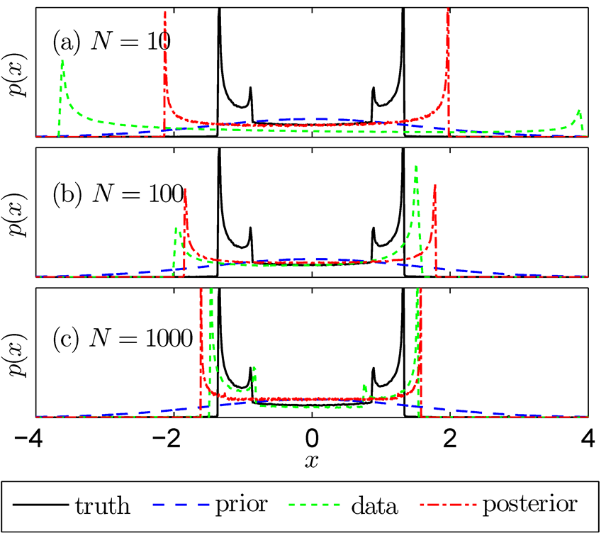
Figure 1: pdfs for linear Bayesian update, from [33]

As the traditional Kalman filter is highly geared towards Gaussian distributions [19], and also its Monte Carlo variant EnKF which was mentioned previously at the beginning of this section tilts towards Gaussianity, we start with a case — already described in [33] — where the the quantity to be identified has a strongly non-Gaussian distribution, shown in black — the ‘truth’ — in Fig. 1. The operator describing the system is the identity — we compute the quantity directly, but there is a Gaussian measurement error. The ‘truth’ was represented as a $12^{\text{th}}$ degree PCE.

We use the methods as described in Subsection 5.5, and here in particular the Eq. (65), the SPKF. The update is repeated several times (here ten times) with new measurements—see Fig. 1. The task is here to identify the distribution labelled as ‘truth’ with ten updates of $N$ samples (where $N=10,100,1000$ was used), and we start with a very broad Gaussian prior (in blue). Here we see the ability of the polynomial based LBU, the PCEKF, to identify highly non-Gaussian distributions, the posterior is shown in red and the pdf estimated from the samples in green; for further details see [33].

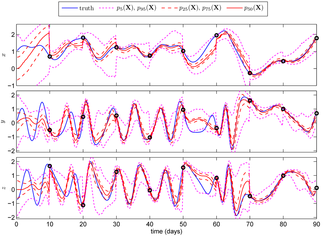
Figure 2: Time evolution of Lorenz-84 state and uncertainty with the LBU, from [33]

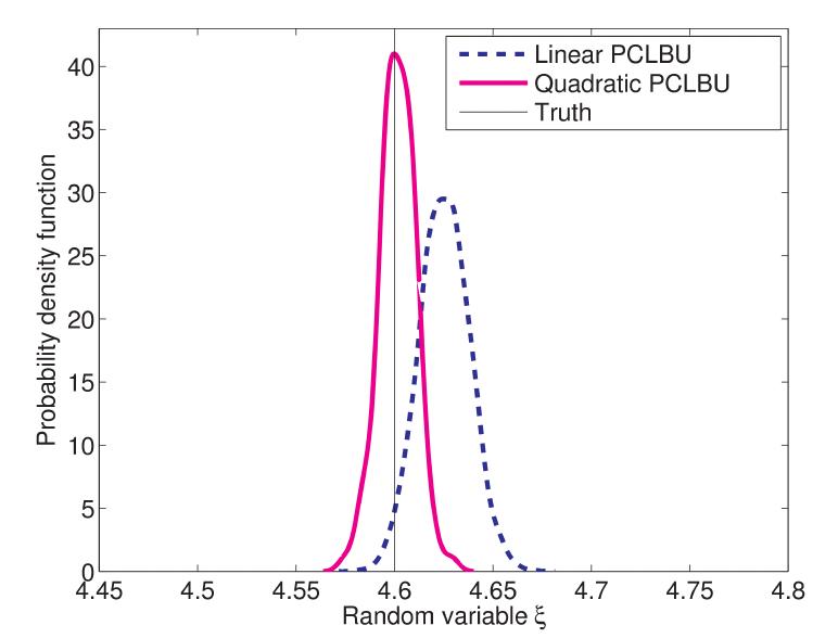
Figure 7: Perturbed observations of the cube of a RV, different updates — linear and quadratic update

The next example is also from [33], where the system is the well-known Lorenz-84 chaotic model, a system of three nonlinear ordinary differential equations operating in the chaotic regime. This is truly an example. Remember that this was originally a model to describe the evolution of some amplitudes of a spherical harmonic expansion of variables describing world climate. As the original scaling of the variables has been kept, the time axis in Fig. 7 is in days. Every ten days a noisy measurement is performed and the state description is updated. In between the state description evolves according to the chaotic dynamic of the system. One may observe from Fig. 7 how the uncertainty — the width of the distribution as given by the quantile lines—shrinks every time a measurement is performed, and then increases again due to the chaotic and hence noisy dynamics. Of course, we did not really measure world climate, but rather simulated the ‘truth’ as well, i.e. a virtual experiment, like the others to follow. More details may be found in [33] and the references therein.

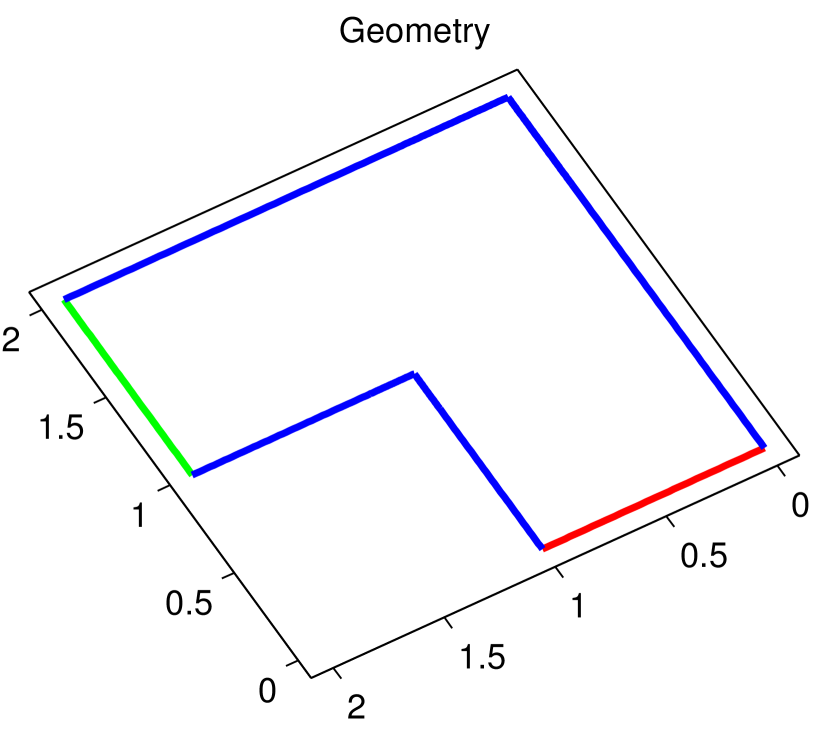
Figure 3: Diffusion domain, from [36]

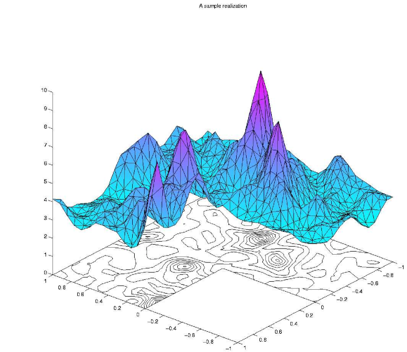
Figure 4: Conductivity field, from [36]

From [36] we take the example shown in Fig. 4, a linear stationary diffusion equation on an L-shaped plane domain. The diffusion coefficient $\kappa$ is to be identified. As argued in [35], it is better to work with $q=\log\kappa$ as the diffusion coefficient has to be positive, but the results are shown in terms of $\kappa$.

One possible realisation of the diffusion coefficient is shown in Fig. 4. More realistically, one should assume that $\kappa$ is a symmetric positive definite tensor field, unless one knows that the diffusion is isotropic. Also in this case one should do the updating on the logarithm. For the sake of simplicity we stay with the scalar case, as there is no principal novelty in the non-isotropic case. The virtual experiments use different right-hand-sides $f$ in Eq. (1), and the measurement is the observation of the solution $u$ averaged over little patches.

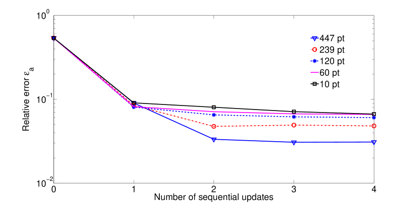
Figure 5: Convergence of identification, from [36]

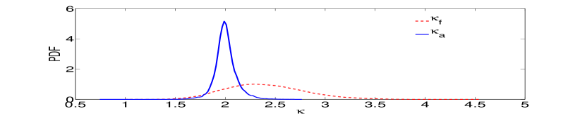
Figure 6: Prior and posterior, from [36]

In Fig. 6 one may observe the decrease of the error with successive updates, but due to measurement error and insufficient information from just a few patches, the curves level off, leaving some residual uncertainty. The pdfs of the diffusion coefficient at some point in the domain before and after the updating is shown in Fig. 6, the ‘true’ value at that point was $\kappa=2$. Further details can be found in [36].

6 More accurate filters

The filter in Eq. (34) resp. Eq. (65) is in some ways the simplest possible one. More accurate filters than the GMKF in Eq. (34) resp. Eq. (36) can be achieved in two ways: for one the subspace $\mathscr{X}_{1}\subset\mathscr{X}_{\sigma(z)}$ in Eq. (31) of affine maps of $\mathchoice{\displaystyle\boldsymbol{z}}{\textstyle\boldsymbol{z}}{\scriptstyle\boldsymbol{z}}{\scriptscriptstyle\boldsymbol{z}}$ may be replaced by increasingly larger subspaces $\mathscr{X}_{\ell}$, and hence more accurate optimal maps $\varpi_{\Psi,\ell}(\mathchoice{\displaystyle\boldsymbol{z}}{\textstyle\boldsymbol{z}}{\scriptstyle\boldsymbol{z}}{\scriptscriptstyle\boldsymbol{z}})$ approximating $\varpi_{\Psi}(\mathchoice{\displaystyle\boldsymbol{z}}{\textstyle\boldsymbol{z}}{\scriptstyle\boldsymbol{z}}{\scriptscriptstyle\boldsymbol{z}})$. This makes for a better approximation of the conditional mean $\mathchoice{\displaystyle\boldsymbol{\bar{x}}}{\textstyle\boldsymbol{\bar{x}}}{\scriptstyle\boldsymbol{\bar{x}}}{\scriptscriptstyle\boldsymbol{\bar{x}}}^{\mathchoice{\displaystyle\boldsymbol{\check{y}}}{\textstyle\boldsymbol{\check{y}}}{\scriptstyle\boldsymbol{\check{y}}}{\scriptscriptstyle\boldsymbol{\check{y}}}}_{a,\ell}:=\varpi_{x,\ell}(\mathchoice{\displaystyle\boldsymbol{\check{y}}}{\textstyle\boldsymbol{\check{y}}}{\scriptstyle\boldsymbol{\check{y}}}{\scriptscriptstyle\boldsymbol{\check{y}}})$ to $\mathchoice{\displaystyle\boldsymbol{\bar{x}}}{\textstyle\boldsymbol{\bar{x}}}{\scriptstyle\boldsymbol{\bar{x}}}{\scriptscriptstyle\boldsymbol{\bar{x}}}^{\mathchoice{\displaystyle\boldsymbol{\check{y}}}{\textstyle\boldsymbol{\check{y}}}{\scriptstyle\boldsymbol{\check{y}}}{\scriptscriptstyle\boldsymbol{\check{y}}}}_{a}$. On the other hand, if one wants $\mathchoice{\displaystyle\mathsfbfit{x}}{\textstyle\mathsfbfit{x}}{\scriptstyle\mathsfbfit{x}}{\scriptscriptstyle\mathsfbfit{x}}_{a}$ to give a better approximation to the Bayesian posterior, the zero-mean part $\mathchoice{\displaystyle\boldsymbol{\tilde{x}}}{\textstyle\boldsymbol{\tilde{x}}}{\scriptstyle\boldsymbol{\tilde{x}}}{\scriptscriptstyle\boldsymbol{\tilde{x}}}^{\mathchoice{\displaystyle\boldsymbol{\check{y}}}{\textstyle\boldsymbol{\check{y}}}{\scriptstyle\boldsymbol{\check{y}}}{\scriptscriptstyle\boldsymbol{\check{y}}}}_{a,\ell}$ has to be possibly transformed.

6.1 Better approximation to the conditional expectation

Let us start by choosing approximating subspaces $\mathscr{X}_{\ell}\subset\mathscr{X}_{\sigma(z)}$ with

$$\mathscr{X}_{1}\subset\mathscr{X}_{\ell}\subset\mathscr{X}_{\sigma(z)}\subset\mathscr{X}.$$

For a RV $\Psi(\mathchoice{\displaystyle\boldsymbol{(}}{\textstyle\boldsymbol{(}}{\scriptstyle\boldsymbol{(}}{\scriptscriptstyle\boldsymbol{(}}x))$, this should give a better approximation $\varpi_{\Psi,\ell}(\mathchoice{\displaystyle\boldsymbol{z}}{\textstyle\boldsymbol{z}}{\scriptstyle\boldsymbol{z}}{\scriptscriptstyle\boldsymbol{z}})$ to $\varpi_{\Psi}(\mathchoice{\displaystyle\boldsymbol{z}}{\textstyle\boldsymbol{z}}{\scriptstyle\boldsymbol{z}}{\scriptscriptstyle\boldsymbol{z}})$ in Eq. (26) than the linear map in Eq. (33). Assuming that the subspaces $\mathscr{X}_{\ell}$ are chosen such that their union is dense in $\mathscr{X}_{\sigma(z)}$,

$$\mathop{\mathrm{cl}}\nolimits\left(\bigcup_{\ell=1}^{\infty}\mathscr{X}_{\ell}\right)=\mathscr{X}_{\sigma(z)},$$ (71)

one may approximate with $\varpi_{\Psi,\ell}$ the optimal map $\varpi_{\Psi}$ to any desired accuracy by taking $\ell$ large enough. This is shown in [28, 29] in general, and in particular for the case when $\mathscr{X}_{\ell}$ is the subspace given by polynomials up to degree $\ell$ in $\mathchoice{\displaystyle\boldsymbol{z}}{\textstyle\boldsymbol{z}}{\scriptstyle\boldsymbol{z}}{\scriptscriptstyle\boldsymbol{z}}$.

Using this in the case $\Psi(\mathchoice{\displaystyle\boldsymbol{x}}{\textstyle\boldsymbol{x}}{\scriptstyle\boldsymbol{x}}{\scriptscriptstyle\boldsymbol{x}})=\mathchoice{\displaystyle\boldsymbol{x}}{\textstyle\boldsymbol{x}}{\scriptstyle\boldsymbol{x}}{\scriptscriptstyle\boldsymbol{x}}$, the linear filter Eq. (36) would then be replaced by

$$\mathchoice{\displaystyle\boldsymbol{x}}{\textstyle\boldsymbol{x}}{\scriptstyle\boldsymbol{x}}{\scriptscriptstyle\boldsymbol{x}}_{a,\ell}(\omega)=\mathchoice{\displaystyle\boldsymbol{x}}{\textstyle\boldsymbol{x}}{\scriptstyle\boldsymbol{x}}{\scriptscriptstyle\boldsymbol{x}}_{f}(\omega)+\varpi_{x,\ell}(\mathchoice{\displaystyle\boldsymbol{\check{y}}}{\textstyle\boldsymbol{\check{y}}}{\scriptstyle\boldsymbol{\check{y}}}{\scriptscriptstyle\boldsymbol{\check{y}}})-\varpi_{x,\ell}(\mathchoice{\displaystyle\boldsymbol{z}}{\textstyle\boldsymbol{z}}{\scriptstyle\boldsymbol{z}}{\scriptscriptstyle\boldsymbol{z}}(\omega))=\varpi_{x,\ell}(\mathchoice{\displaystyle\boldsymbol{\check{y}}}{\textstyle\boldsymbol{\check{y}}}{\scriptstyle\boldsymbol{\check{y}}}{\scriptscriptstyle\boldsymbol{\check{y}}})+(\mathchoice{\displaystyle\boldsymbol{x}}{\textstyle\boldsymbol{x}}{\scriptstyle\boldsymbol{x}}{\scriptscriptstyle\boldsymbol{x}}_{f}(\omega)-\varpi_{x,\ell}(\mathchoice{\displaystyle\boldsymbol{z}}{\textstyle\boldsymbol{z}}{\scriptstyle\boldsymbol{z}}{\scriptscriptstyle\boldsymbol{z}}(\omega))),$$ (72)

which is a non-linear filter as an approximation to the CEM-filter Eq. (29). Observe that in general this will only result in the RV $\mathchoice{\displaystyle\boldsymbol{x}}{\textstyle\boldsymbol{x}}{\scriptstyle\boldsymbol{x}}{\scriptscriptstyle\boldsymbol{x}}_{a,\ell}$ having a posterior mean $\varpi_{x,\ell}(\mathchoice{\displaystyle\boldsymbol{\check{y}}}{\textstyle\boldsymbol{\check{y}}}{\scriptstyle\boldsymbol{\check{y}}}{\scriptscriptstyle\boldsymbol{\check{y}}})=\mathchoice{\displaystyle\boldsymbol{\bar{x}}}{\textstyle\boldsymbol{\bar{x}}}{\scriptstyle\boldsymbol{\bar{x}}}{\scriptscriptstyle\boldsymbol{\bar{x}}}^{\mathchoice{\displaystyle\boldsymbol{\check{y}}}{\textstyle\boldsymbol{\check{y}}}{\scriptstyle\boldsymbol{\check{y}}}{\scriptscriptstyle\boldsymbol{\check{y}}}}_{a,\ell}$ closer to the posterior Bayesian mean $\mathchoice{\displaystyle\boldsymbol{\bar{x}}}{\textstyle\boldsymbol{\bar{x}}}{\scriptstyle\boldsymbol{\bar{x}}}{\scriptscriptstyle\boldsymbol{\bar{x}}}^{\mathchoice{\displaystyle\boldsymbol{\check{y}}}{\textstyle\boldsymbol{\check{y}}}{\scriptstyle\boldsymbol{\check{y}}}{\scriptscriptstyle\boldsymbol{\check{y}}}}_{a}$. In case the density condition Eq. (71) is satisfied, one obtains convergence $\mathchoice{\displaystyle\boldsymbol{\bar{x}}}{\textstyle\boldsymbol{\bar{x}}}{\scriptstyle\boldsymbol{\bar{x}}}{\scriptscriptstyle\boldsymbol{\bar{x}}}^{\mathchoice{\displaystyle\boldsymbol{\check{y}}}{\textstyle\boldsymbol{\check{y}}}{\scriptstyle\boldsymbol{\check{y}}}{\scriptscriptstyle\boldsymbol{\check{y}}}}_{a,\ell}\to\mathchoice{\displaystyle\boldsymbol{\bar{x}}}{\textstyle\boldsymbol{\bar{x}}}{\scriptstyle\boldsymbol{\bar{x}}}{\scriptscriptstyle\boldsymbol{\bar{x}}}^{\mathchoice{\displaystyle\boldsymbol{\check{y}}}{\textstyle\boldsymbol{\check{y}}}{\scriptstyle\boldsymbol{\check{y}}}{\scriptscriptstyle\boldsymbol{\check{y}}}}_{a}$ as $\ell\to\infty$.

To introduce the nonlinear filter as just sketched, one may look shortly at a very simplified example, identifying a value, where only the third power of the value plus a Gaussian error RV is observed. All updates follow Eq. (72), but the update map is computed with different accuracy.

Shown are the pdfs produced by the linear filter according to Eq. (65) — Linear polynomial chaos Bayesian update (Linear PCBU) — a special form of Eq. (72), and using polynomials up to order two, the quadratic polynomial chaos Bayesian update (QPCBU). One may observe that due to the nonlinear observation, the differences between the linear filters and the quadratic one are already significant, the QPCBU yielding a better update.

6.2 Transformation of the zero-mean part

Hence, if on the other hand one wants to construct a RV which matches the full posterior Bayesian distribution, one has to look at the zero mean part from Eq. (29)

$$\mathchoice{\displaystyle\boldsymbol{\tilde{x}}}{\textstyle\boldsymbol{\tilde{x}}}{\scriptstyle\boldsymbol{\tilde{x}}}{\scriptscriptstyle\boldsymbol{\tilde{x}}}^{\mathchoice{\displaystyle\boldsymbol{\check{y}}}{\textstyle\boldsymbol{\check{y}}}{\scriptstyle\boldsymbol{\check{y}}}{\scriptscriptstyle\boldsymbol{\check{y}}}}_{a}(\mathchoice{\displaystyle\boldsymbol{\xi}}{\textstyle\boldsymbol{\xi}}{\scriptstyle\boldsymbol{\xi}}{\scriptscriptstyle\boldsymbol{\xi}},\mathchoice{\displaystyle\boldsymbol{\eta}}{\textstyle\boldsymbol{\eta}}{\scriptstyle\boldsymbol{\eta}}{\scriptscriptstyle\boldsymbol{\eta}})=\mathchoice{\displaystyle\boldsymbol{x}}{\textstyle\boldsymbol{x}}{\scriptstyle\boldsymbol{x}}{\scriptscriptstyle\boldsymbol{x}}_{f}(\mathchoice{\displaystyle\boldsymbol{\xi}}{\textstyle\boldsymbol{\xi}}{\scriptstyle\boldsymbol{\xi}}{\scriptscriptstyle\boldsymbol{\xi}})-\varpi_{x}(\mathchoice{\displaystyle\boldsymbol{z}}{\textstyle\boldsymbol{z}}{\scriptstyle\boldsymbol{z}}{\scriptscriptstyle\boldsymbol{z}}(\mathchoice{\displaystyle\boldsymbol{\xi}}{\textstyle\boldsymbol{\xi}}{\scriptstyle\boldsymbol{\xi}}{\scriptscriptstyle\boldsymbol{\xi}},\mathchoice{\displaystyle\boldsymbol{\eta}}{\textstyle\boldsymbol{\eta}}{\scriptstyle\boldsymbol{\eta}}{\scriptscriptstyle\boldsymbol{\eta}})),$$ (73)

which is essentially what is left from the orthogonal projection. For an actual computation, one would choose a finite $\ell$ and use Eq. (72). This RV $\mathchoice{\displaystyle\boldsymbol{\tilde{x}}}{\textstyle\boldsymbol{\tilde{x}}}{\scriptstyle\boldsymbol{\tilde{x}}}{\scriptscriptstyle\boldsymbol{\tilde{x}}}^{\mathchoice{\displaystyle\boldsymbol{\check{y}}}{\textstyle\boldsymbol{\check{y}}}{\scriptstyle\boldsymbol{\check{y}}}{\scriptscriptstyle\boldsymbol{\check{y}}}}_{a}$ will have to be transformed further.

From Eq. (35) one has the covariance $\mathchoice{\displaystyle\boldsymbol{C}}{\textstyle\boldsymbol{C}}{\scriptstyle\boldsymbol{C}}{\scriptscriptstyle\boldsymbol{C}}_{x_{a}}$ of $\mathchoice{\displaystyle\boldsymbol{\tilde{x}}}{\textstyle\boldsymbol{\tilde{x}}}{\scriptstyle\boldsymbol{\tilde{x}}}{\scriptscriptstyle\boldsymbol{\tilde{x}}}^{\mathchoice{\displaystyle\boldsymbol{\check{y}}}{\textstyle\boldsymbol{\check{y}}}{\scriptstyle\boldsymbol{\check{y}}}{\scriptscriptstyle\boldsymbol{\check{y}}}}_{a,1}$. A similar computation can be performed, at least numerically, for $\mathchoice{\displaystyle\boldsymbol{\tilde{x}}}{\textstyle\boldsymbol{\tilde{x}}}{\scriptstyle\boldsymbol{\tilde{x}}}{\scriptscriptstyle\boldsymbol{\tilde{x}}}^{\mathchoice{\displaystyle\boldsymbol{\check{y}}}{\textstyle\boldsymbol{\check{y}}}{\scriptstyle\boldsymbol{\check{y}}}{\scriptscriptstyle\boldsymbol{\check{y}}}}_{a}$ in Eq. (73), giving $\mathchoice{\displaystyle\boldsymbol{\hat{C}}}{\textstyle\boldsymbol{\hat{C}}}{\scriptstyle\boldsymbol{\hat{C}}}{\scriptscriptstyle\boldsymbol{\hat{C}}}_{x_{a}}=\mathbb{E}\left(\mathchoice{\displaystyle\boldsymbol{\tilde{x}}}{\textstyle\boldsymbol{\tilde{x}}}{\scriptstyle\boldsymbol{\tilde{x}}}{\scriptscriptstyle\boldsymbol{\tilde{x}}}^{\mathchoice{\displaystyle\boldsymbol{\check{y}}}{\textstyle\boldsymbol{\check{y}}}{\scriptstyle\boldsymbol{\check{y}}}{\scriptscriptstyle\boldsymbol{\check{y}}}}_{a}\otimes\mathchoice{\displaystyle\boldsymbol{\tilde{x}}}{\textstyle\boldsymbol{\tilde{x}}}{\scriptstyle\boldsymbol{\tilde{x}}}{\scriptscriptstyle\boldsymbol{\tilde{x}}}^{\mathchoice{\displaystyle\boldsymbol{\check{y}}}{\textstyle\boldsymbol{\check{y}}}{\scriptstyle\boldsymbol{\check{y}}}{\scriptscriptstyle\boldsymbol{\check{y}}}}_{a}\right)$.

On the other hand, one may compute the correct value of the posterior covariance to any degree of accuracy with an optimal map. While in section 4.2.1 we have computed the optimal map $\varpi_{\Psi}$ for $\Psi(\mathchoice{\displaystyle\boldsymbol{x}}{\textstyle\boldsymbol{x}}{\scriptstyle\boldsymbol{x}}{\scriptscriptstyle\boldsymbol{x}})=\mathchoice{\displaystyle\boldsymbol{x}}{\textstyle\boldsymbol{x}}{\scriptstyle\boldsymbol{x}}{\scriptscriptstyle\boldsymbol{x}}$, now we may take $\Psi(x)=\mathchoice{\displaystyle\boldsymbol{x}}{\textstyle\boldsymbol{x}}{\scriptstyle\boldsymbol{x}}{\scriptscriptstyle\boldsymbol{x}}\otimes\mathchoice{\displaystyle\boldsymbol{x}}{\textstyle\boldsymbol{x}}{\scriptstyle\boldsymbol{x}}{\scriptscriptstyle\boldsymbol{x}}$ to obtain an optimal map $\varpi_{x\otimes x}$. This then gives

$$\mathchoice{\displaystyle\boldsymbol{C}}{\textstyle\boldsymbol{C}}{\scriptstyle\boldsymbol{C}}{\scriptscriptstyle\boldsymbol{C}}_{x_{a}}=\mathbb{E}\left(\mathchoice{\displaystyle\boldsymbol{x}}{\textstyle\boldsymbol{x}}{\scriptstyle\boldsymbol{x}}{\scriptscriptstyle\boldsymbol{x}}_{f}\otimes\mathchoice{\displaystyle\boldsymbol{x}}{\textstyle\boldsymbol{x}}{\scriptstyle\boldsymbol{x}}{\scriptscriptstyle\boldsymbol{x}}_{f}|\mathchoice{\displaystyle\boldsymbol{\check{y}}}{\textstyle\boldsymbol{\check{y}}}{\scriptstyle\boldsymbol{\check{y}}}{\scriptscriptstyle\boldsymbol{\check{y}}}\right)-\mathchoice{\displaystyle\boldsymbol{\bar{x}}}{\textstyle\boldsymbol{\bar{x}}}{\scriptstyle\boldsymbol{\bar{x}}}{\scriptscriptstyle\boldsymbol{\bar{x}}}^{\mathchoice{\displaystyle\boldsymbol{\check{y}}}{\textstyle\boldsymbol{\check{y}}}{\scriptstyle\boldsymbol{\check{y}}}{\scriptscriptstyle\boldsymbol{\check{y}}}}_{a}\otimes\mathchoice{\displaystyle\boldsymbol{\bar{x}}}{\textstyle\boldsymbol{\bar{x}}}{\scriptstyle\boldsymbol{\bar{x}}}{\scriptscriptstyle\boldsymbol{\bar{x}}}^{\mathchoice{\displaystyle\boldsymbol{\check{y}}}{\textstyle\boldsymbol{\check{y}}}{\scriptstyle\boldsymbol{\check{y}}}{\scriptscriptstyle\boldsymbol{\check{y}}}}_{a}=\varpi_{x\otimes x}(\mathchoice{\displaystyle\boldsymbol{\check{y}}}{\textstyle\boldsymbol{\check{y}}}{\scriptstyle\boldsymbol{\check{y}}}{\scriptscriptstyle\boldsymbol{\check{y}}})-\mathchoice{\displaystyle\boldsymbol{\bar{x}}}{\textstyle\boldsymbol{\bar{x}}}{\scriptstyle\boldsymbol{\bar{x}}}{\scriptscriptstyle\boldsymbol{\bar{x}}}^{\mathchoice{\displaystyle\boldsymbol{\check{y}}}{\textstyle\boldsymbol{\check{y}}}{\scriptstyle\boldsymbol{\check{y}}}{\scriptscriptstyle\boldsymbol{\check{y}}}}_{a}\otimes\mathchoice{\displaystyle\boldsymbol{\bar{x}}}{\textstyle\boldsymbol{\bar{x}}}{\scriptstyle\boldsymbol{\bar{x}}}{\scriptscriptstyle\boldsymbol{\bar{x}}}^{\mathchoice{\displaystyle\boldsymbol{\check{y}}}{\textstyle\boldsymbol{\check{y}}}{\scriptstyle\boldsymbol{\check{y}}}{\scriptscriptstyle\boldsymbol{\check{y}}}}_{a}.$$ (74)

For a numerical approximation over $\mathscr{X}_{\ell}$ this would similarly result in an approximation $\mathchoice{\displaystyle\boldsymbol{C}}{\textstyle\boldsymbol{C}}{\scriptstyle\boldsymbol{C}}{\scriptscriptstyle\boldsymbol{C}}_{x_{a},\ell}$. Both the former $\mathchoice{\displaystyle\boldsymbol{\hat{C}}}{\textstyle\boldsymbol{\hat{C}}}{\scriptstyle\boldsymbol{\hat{C}}}{\scriptscriptstyle\boldsymbol{\hat{C}}}_{x_{a}}$ as well as $\mathchoice{\displaystyle\boldsymbol{C}}{\textstyle\boldsymbol{C}}{\scriptstyle\boldsymbol{C}}{\scriptscriptstyle\boldsymbol{C}}_{x_{a}}$ in Eq. (83) are spd matrices, hence have a square root. Therefore, when considering the following RV

$$\mathchoice{\displaystyle\boldsymbol{x}}{\textstyle\boldsymbol{x}}{\scriptstyle\boldsymbol{x}}{\scriptscriptstyle\boldsymbol{x}}_{a,\text{cov}}(\mathchoice{\displaystyle\boldsymbol{\xi}}{\textstyle\boldsymbol{\xi}}{\scriptstyle\boldsymbol{\xi}}{\scriptscriptstyle\boldsymbol{\xi}},\mathchoice{\displaystyle\boldsymbol{\eta}}{\textstyle\boldsymbol{\eta}}{\scriptstyle\boldsymbol{\eta}}{\scriptscriptstyle\boldsymbol{\eta}})=\varpi_{x}(\mathchoice{\displaystyle\boldsymbol{\check{y}}}{\textstyle\boldsymbol{\check{y}}}{\scriptstyle\boldsymbol{\check{y}}}{\scriptscriptstyle\boldsymbol{\check{y}}})+\mathchoice{\displaystyle\boldsymbol{C}}{\textstyle\boldsymbol{C}}{\scriptstyle\boldsymbol{C}}{\scriptscriptstyle\boldsymbol{C}}_{x_{a}}^{1/2}\,\mathchoice{\displaystyle\boldsymbol{\hat{C}}}{\textstyle\boldsymbol{\hat{C}}}{\scriptstyle\boldsymbol{\hat{C}}}{\scriptscriptstyle\boldsymbol{\hat{C}}}_{x_{a}}^{-1/2}(\mathchoice{\displaystyle\boldsymbol{\tilde{x}}}{\textstyle\boldsymbol{\tilde{x}}}{\scriptstyle\boldsymbol{\tilde{x}}}{\scriptscriptstyle\boldsymbol{\tilde{x}}}^{\mathchoice{\displaystyle\boldsymbol{\check{y}}}{\textstyle\boldsymbol{\check{y}}}{\scriptstyle\boldsymbol{\check{y}}}{\scriptscriptstyle\boldsymbol{\check{y}}}}_{a}(\mathchoice{\displaystyle\boldsymbol{\xi}}{\textstyle\boldsymbol{\xi}}{\scriptstyle\boldsymbol{\xi}}{\scriptscriptstyle\boldsymbol{\xi}},\mathchoice{\displaystyle\boldsymbol{\eta}}{\textstyle\boldsymbol{\eta}}{\scriptstyle\boldsymbol{\eta}}{\scriptscriptstyle\boldsymbol{\eta}})),$$ (75)

with $\mathchoice{\displaystyle\boldsymbol{\tilde{x}}}{\textstyle\boldsymbol{\tilde{x}}}{\scriptstyle\boldsymbol{\tilde{x}}}{\scriptscriptstyle\boldsymbol{\tilde{x}}}^{\mathchoice{\displaystyle\boldsymbol{\check{y}}}{\textstyle\boldsymbol{\check{y}}}{\scriptstyle\boldsymbol{\check{y}}}{\scriptscriptstyle\boldsymbol{\check{y}}}}_{a}$ from Eq. (73), it is obvious that it has the required covariance $\mathchoice{\displaystyle\boldsymbol{C}}{\textstyle\boldsymbol{C}}{\scriptstyle\boldsymbol{C}}{\scriptscriptstyle\boldsymbol{C}}_{x_{a}}$ in Eq. (74).

While Eq. (29), Eq. (36), or Eq. (72) are transformations of $\mathchoice{\displaystyle\mathsfbfit{x}}{\textstyle\mathsfbfit{x}}{\scriptstyle\mathsfbfit{x}}{\scriptscriptstyle\mathsfbfit{x}}_{f}$ to $\mathchoice{\displaystyle\mathsfbfit{x}}{\textstyle\mathsfbfit{x}}{\scriptstyle\mathsfbfit{x}}{\scriptscriptstyle\mathsfbfit{x}}_{a}$ through a simple shift, in Eq. (75) there is an additional linear transformation of the zero mean part $\mathchoice{\displaystyle\boldsymbol{\tilde{x}}}{\textstyle\boldsymbol{\tilde{x}}}{\scriptstyle\boldsymbol{\tilde{x}}}{\scriptscriptstyle\boldsymbol{\tilde{x}}}^{\mathchoice{\displaystyle\boldsymbol{\check{y}}}{\textstyle\boldsymbol{\check{y}}}{\scriptstyle\boldsymbol{\check{y}}}{\scriptscriptstyle\boldsymbol{\check{y}}}}_{a}$. Although the first two moments of $\mathchoice{\displaystyle\boldsymbol{x}}{\textstyle\boldsymbol{x}}{\scriptstyle\boldsymbol{x}}{\scriptscriptstyle\boldsymbol{x}}_{a,\text{cov}}$ in Eq. (75) are correct, it does not seem so simple to proceed further.

In the following, we have two objectives. For one, we want an assimilated RV which matches the Bayesian posterior even better, beyond the first two moments, and on the other hand we do not need so many RVs $\mathchoice{\displaystyle\boldsymbol{\xi}}{\textstyle\boldsymbol{\xi}}{\scriptstyle\boldsymbol{\xi}}{\scriptscriptstyle\boldsymbol{\xi}}$ and $\mathchoice{\displaystyle\boldsymbol{\eta}}{\textstyle\boldsymbol{\eta}}{\scriptstyle\boldsymbol{\eta}}{\scriptscriptstyle\boldsymbol{\eta}}$ to describe the RV $\mathchoice{\displaystyle\boldsymbol{\tilde{x}}}{\textstyle\boldsymbol{\tilde{x}}}{\scriptstyle\boldsymbol{\tilde{x}}}{\scriptscriptstyle\boldsymbol{\tilde{x}}}^{\mathchoice{\displaystyle\boldsymbol{\check{y}}}{\textstyle\boldsymbol{\check{y}}}{\scriptstyle\boldsymbol{\check{y}}}{\scriptscriptstyle\boldsymbol{\check{y}}}}_{a}$. For the following assume that $\mathchoice{\displaystyle\boldsymbol{\xi}}{\textstyle\boldsymbol{\xi}}{\scriptstyle\boldsymbol{\xi}}{\scriptscriptstyle\boldsymbol{\xi}}$ and $\mathchoice{\displaystyle\boldsymbol{\eta}}{\textstyle\boldsymbol{\eta}}{\scriptstyle\boldsymbol{\eta}}{\scriptscriptstyle\boldsymbol{\eta}}$ are centred normalised jointly Gaussian and uncorrelated — hence independent — in the unconditional expectation $\mathbb{E}\left(\cdot\right)$. They are not necessarily uncorrelated in the conditional expectation $\mathbb{E}\left(\cdot|\mathchoice{\displaystyle\boldsymbol{\check{y}}}{\textstyle\boldsymbol{\check{y}}}{\scriptstyle\boldsymbol{\check{y}}}{\scriptscriptstyle\boldsymbol{\check{y}}}\right)$ though.

To start with this latter task, perform a singular value decomposition on the $M\times(L+K)$ matrix $\mathchoice{\displaystyle\boldsymbol{R}}{\textstyle\boldsymbol{R}}{\scriptstyle\boldsymbol{R}}{\scriptscriptstyle\boldsymbol{R}}$, where normally $L+K\geq M$:

$$\mathchoice{\displaystyle\boldsymbol{R}}{\textstyle\boldsymbol{R}}{\scriptstyle\boldsymbol{R}}{\scriptscriptstyle\boldsymbol{R}}=[\mathbb{E}\left(\mathchoice{\displaystyle\boldsymbol{\tilde{x}}}{\textstyle\boldsymbol{\tilde{x}}}{\scriptstyle\boldsymbol{\tilde{x}}}{\scriptscriptstyle\boldsymbol{\tilde{x}}}^{\mathchoice{\displaystyle\boldsymbol{\check{y}}}{\textstyle\boldsymbol{\check{y}}}{\scriptstyle\boldsymbol{\check{y}}}{\scriptscriptstyle\boldsymbol{\check{y}}}}_{a}\otimes\mathchoice{\displaystyle\boldsymbol{\xi}}{\textstyle\boldsymbol{\xi}}{\scriptstyle\boldsymbol{\xi}}{\scriptscriptstyle\boldsymbol{\xi}}|\mathchoice{\displaystyle\boldsymbol{\check{y}}}{\textstyle\boldsymbol{\check{y}}}{\scriptstyle\boldsymbol{\check{y}}}{\scriptscriptstyle\boldsymbol{\check{y}}}\right),\mathbb{E}\left(\mathchoice{\displaystyle\boldsymbol{\tilde{x}}}{\textstyle\boldsymbol{\tilde{x}}}{\scriptstyle\boldsymbol{\tilde{x}}}{\scriptscriptstyle\boldsymbol{\tilde{x}}}^{\mathchoice{\displaystyle\boldsymbol{\check{y}}}{\textstyle\boldsymbol{\check{y}}}{\scriptstyle\boldsymbol{\check{y}}}{\scriptscriptstyle\boldsymbol{\check{y}}}}_{a}\otimes\mathchoice{\displaystyle\boldsymbol{\eta}}{\textstyle\boldsymbol{\eta}}{\scriptstyle\boldsymbol{\eta}}{\scriptscriptstyle\boldsymbol{\eta}}|\mathchoice{\displaystyle\boldsymbol{\check{y}}}{\textstyle\boldsymbol{\check{y}}}{\scriptstyle\boldsymbol{\check{y}}}{\scriptscriptstyle\boldsymbol{\check{y}}}\right)]=\mathchoice{\displaystyle\boldsymbol{U}}{\textstyle\boldsymbol{U}}{\scriptstyle\boldsymbol{U}}{\scriptscriptstyle\boldsymbol{U}}\mathchoice{\displaystyle\boldsymbol{\Sigma}}{\textstyle\boldsymbol{\Sigma}}{\scriptstyle\boldsymbol{\Sigma}}{\scriptscriptstyle\boldsymbol{\Sigma}}\mathchoice{\displaystyle\boldsymbol{V}}{\textstyle\boldsymbol{V}}{\scriptstyle\boldsymbol{V}}{\scriptscriptstyle\boldsymbol{V}}^{\mathchoice{\displaystyle\mathsf{T}}{\textstyle\mathsf{T}}{\scriptstyle\mathsf{T}}{\scriptscriptstyle\mathsf{T}}};$$ (76)

here $\mathchoice{\displaystyle\boldsymbol{\Sigma}}{\textstyle\boldsymbol{\Sigma}}{\scriptstyle\boldsymbol{\Sigma}}{\scriptscriptstyle\boldsymbol{\Sigma}}$ is the non-singular diagonal $R\times R$-matrix of non-zero singular values, with $R\leq M$ the rank of $\mathchoice{\displaystyle\boldsymbol{R}}{\textstyle\boldsymbol{R}}{\scriptstyle\boldsymbol{R}}{\scriptscriptstyle\boldsymbol{R}}$, and $\mathchoice{\displaystyle\boldsymbol{U}}{\textstyle\boldsymbol{U}}{\scriptstyle\boldsymbol{U}}{\scriptscriptstyle\boldsymbol{U}}$ is a $M\times R$ orthogonal matrix ($\mathchoice{\displaystyle\boldsymbol{U}}{\textstyle\boldsymbol{U}}{\scriptstyle\boldsymbol{U}}{\scriptscriptstyle\boldsymbol{U}}^{\mathchoice{\displaystyle\mathsf{T}}{\textstyle\mathsf{T}}{\scriptstyle\mathsf{T}}{\scriptscriptstyle\mathsf{T}}}\mathchoice{\displaystyle\boldsymbol{U}}{\textstyle\boldsymbol{U}}{\scriptstyle\boldsymbol{U}}{\scriptscriptstyle\boldsymbol{U}}=\mathchoice{\displaystyle\boldsymbol{\mathrm{I}}}{\textstyle\boldsymbol{\mathrm{I}}}{\scriptstyle\boldsymbol{\mathrm{I}}}{\scriptscriptstyle\boldsymbol{\mathrm{I}}}_{R}$), and $\mathchoice{\displaystyle\boldsymbol{V}}{\textstyle\boldsymbol{V}}{\scriptstyle\boldsymbol{V}}{\scriptscriptstyle\boldsymbol{V}}$ a $(L+K)\times R$ orthogonal matrix ($\mathchoice{\displaystyle\boldsymbol{V}}{\textstyle\boldsymbol{V}}{\scriptstyle\boldsymbol{V}}{\scriptscriptstyle\boldsymbol{V}}^{\mathchoice{\displaystyle\mathsf{T}}{\textstyle\mathsf{T}}{\scriptstyle\mathsf{T}}{\scriptscriptstyle\mathsf{T}}}\mathchoice{\displaystyle\boldsymbol{V}}{\textstyle\boldsymbol{V}}{\scriptstyle\boldsymbol{V}}{\scriptscriptstyle\boldsymbol{V}}=\mathchoice{\displaystyle\boldsymbol{\mathrm{I}}}{\textstyle\boldsymbol{\mathrm{I}}}{\scriptstyle\boldsymbol{\mathrm{I}}}{\scriptscriptstyle\boldsymbol{\mathrm{I}}}_{R}$). The conditional expectation has to be performed w.r.t. $\mathchoice{\displaystyle\boldsymbol{\xi}}{\textstyle\boldsymbol{\xi}}{\scriptstyle\boldsymbol{\xi}}{\scriptscriptstyle\boldsymbol{\xi}}$ and $\mathchoice{\displaystyle\boldsymbol{\eta}}{\textstyle\boldsymbol{\eta}}{\scriptstyle\boldsymbol{\eta}}{\scriptscriptstyle\boldsymbol{\eta}}$ by computing the optimal maps $\varpi_{\Psi}$ corresponding to $\Psi(\mathchoice{\displaystyle\boldsymbol{\xi}}{\textstyle\boldsymbol{\xi}}{\scriptstyle\boldsymbol{\xi}}{\scriptscriptstyle\boldsymbol{\xi}},\mathchoice{\displaystyle\boldsymbol{\eta}}{\textstyle\boldsymbol{\eta}}{\scriptstyle\boldsymbol{\eta}}{\scriptscriptstyle\boldsymbol{\eta}})=\mathchoice{\displaystyle\boldsymbol{\tilde{x}}}{\textstyle\boldsymbol{\tilde{x}}}{\scriptstyle\boldsymbol{\tilde{x}}}{\scriptscriptstyle\boldsymbol{\tilde{x}}}^{\mathchoice{\displaystyle\boldsymbol{\check{y}}}{\textstyle\boldsymbol{\check{y}}}{\scriptstyle\boldsymbol{\check{y}}}{\scriptscriptstyle\boldsymbol{\check{y}}}}_{a}\otimes\mathchoice{\displaystyle\boldsymbol{\xi}}{\textstyle\boldsymbol{\xi}}{\scriptstyle\boldsymbol{\xi}}{\scriptscriptstyle\boldsymbol{\xi}}$ and $\Psi(\mathchoice{\displaystyle\boldsymbol{\xi}}{\textstyle\boldsymbol{\xi}}{\scriptstyle\boldsymbol{\xi}}{\scriptscriptstyle\boldsymbol{\xi}},\mathchoice{\displaystyle\boldsymbol{\eta}}{\textstyle\boldsymbol{\eta}}{\scriptstyle\boldsymbol{\eta}}{\scriptscriptstyle\boldsymbol{\eta}})=\mathchoice{\displaystyle\boldsymbol{\tilde{x}}}{\textstyle\boldsymbol{\tilde{x}}}{\scriptstyle\boldsymbol{\tilde{x}}}{\scriptscriptstyle\boldsymbol{\tilde{x}}}^{\mathchoice{\displaystyle\boldsymbol{\check{y}}}{\textstyle\boldsymbol{\check{y}}}{\scriptstyle\boldsymbol{\check{y}}}{\scriptscriptstyle\boldsymbol{\check{y}}}}_{a}\otimes\mathchoice{\displaystyle\boldsymbol{\eta}}{\textstyle\boldsymbol{\eta}}{\scriptstyle\boldsymbol{\eta}}{\scriptscriptstyle\boldsymbol{\eta}}$, denoted by $\varpi_{\mathchoice{\displaystyle\boldsymbol{\tilde{x}}}{\textstyle\boldsymbol{\tilde{x}}}{\scriptstyle\boldsymbol{\tilde{x}}}{\scriptscriptstyle\boldsymbol{\tilde{x}}}\xi}$ and $\varpi_{\mathchoice{\displaystyle\boldsymbol{\tilde{x}}}{\textstyle\boldsymbol{\tilde{x}}}{\scriptstyle\boldsymbol{\tilde{x}}}{\scriptscriptstyle\boldsymbol{\tilde{x}}}\eta}$ such that

$$\mathbb{E}\left(\mathchoice{\displaystyle\boldsymbol{\tilde{x}}}{\textstyle\boldsymbol{\tilde{x}}}{\scriptstyle\boldsymbol{\tilde{x}}}{\scriptscriptstyle\boldsymbol{\tilde{x}}}^{\mathchoice{\displaystyle\boldsymbol{\check{y}}}{\textstyle\boldsymbol{\check{y}}}{\scriptstyle\boldsymbol{\check{y}}}{\scriptscriptstyle\boldsymbol{\check{y}}}}_{a}\otimes\mathchoice{\displaystyle\boldsymbol{\xi}}{\textstyle\boldsymbol{\xi}}{\scriptstyle\boldsymbol{\xi}}{\scriptscriptstyle\boldsymbol{\xi}}|\mathchoice{\displaystyle\boldsymbol{\check{y}}}{\textstyle\boldsymbol{\check{y}}}{\scriptstyle\boldsymbol{\check{y}}}{\scriptscriptstyle\boldsymbol{\check{y}}}\right)=\varpi_{\mathchoice{\displaystyle\boldsymbol{\tilde{x}}}{\textstyle\boldsymbol{\tilde{x}}}{\scriptstyle\boldsymbol{\tilde{x}}}{\scriptscriptstyle\boldsymbol{\tilde{x}}}\xi}(\mathchoice{\displaystyle\boldsymbol{\check{y}}}{\textstyle\boldsymbol{\check{y}}}{\scriptstyle\boldsymbol{\check{y}}}{\scriptscriptstyle\boldsymbol{\check{y}}})\qquad\text{and}\qquad\mathbb{E}\left(\mathchoice{\displaystyle\boldsymbol{\tilde{x}}}{\textstyle\boldsymbol{\tilde{x}}}{\scriptstyle\boldsymbol{\tilde{x}}}{\scriptscriptstyle\boldsymbol{\tilde{x}}}^{\mathchoice{\displaystyle\boldsymbol{\check{y}}}{\textstyle\boldsymbol{\check{y}}}{\scriptstyle\boldsymbol{\check{y}}}{\scriptscriptstyle\boldsymbol{\check{y}}}}_{a}\otimes\mathchoice{\displaystyle\boldsymbol{\eta}}{\textstyle\boldsymbol{\eta}}{\scriptstyle\boldsymbol{\eta}}{\scriptscriptstyle\boldsymbol{\eta}}|\mathchoice{\displaystyle\boldsymbol{\check{y}}}{\textstyle\boldsymbol{\check{y}}}{\scriptstyle\boldsymbol{\check{y}}}{\scriptscriptstyle\boldsymbol{\check{y}}}\right)=\varpi_{\mathchoice{\displaystyle\boldsymbol{\tilde{x}}}{\textstyle\boldsymbol{\tilde{x}}}{\scriptstyle\boldsymbol{\tilde{x}}}{\scriptscriptstyle\boldsymbol{\tilde{x}}}\eta}(\mathchoice{\displaystyle\boldsymbol{\check{y}}}{\textstyle\boldsymbol{\check{y}}}{\scriptstyle\boldsymbol{\check{y}}}{\scriptscriptstyle\boldsymbol{\check{y}}}).$$ (77)

Similarly, perform an eigenvalue decomposition of the new $\mathchoice{\displaystyle\boldsymbol{\xi}}{\textstyle\boldsymbol{\xi}}{\scriptstyle\boldsymbol{\xi}}{\scriptscriptstyle\boldsymbol{\xi}},\mathchoice{\displaystyle\boldsymbol{\eta}}{\textstyle\boldsymbol{\eta}}{\scriptstyle\boldsymbol{\eta}}{\scriptscriptstyle\boldsymbol{\eta}}$ correlation matrix

$$\mathchoice{\displaystyle\boldsymbol{C}}{\textstyle\boldsymbol{C}}{\scriptstyle\boldsymbol{C}}{\scriptscriptstyle\boldsymbol{C}}^{\mathchoice{\displaystyle\boldsymbol{\check{y}}}{\textstyle\boldsymbol{\check{y}}}{\scriptstyle\boldsymbol{\check{y}}}{\scriptscriptstyle\boldsymbol{\check{y}}}}_{(\xi\eta)}:=\begin{bmatrix}\mathbb{E}\left(\mathchoice{\displaystyle\boldsymbol{\xi}}{\textstyle\boldsymbol{\xi}}{\scriptstyle\boldsymbol{\xi}}{\scriptscriptstyle\boldsymbol{\xi}}\otimes\mathchoice{\displaystyle\boldsymbol{\xi}}{\textstyle\boldsymbol{\xi}}{\scriptstyle\boldsymbol{\xi}}{\scriptscriptstyle\boldsymbol{\xi}}|\mathchoice{\displaystyle\boldsymbol{\check{y}}}{\textstyle\boldsymbol{\check{y}}}{\scriptstyle\boldsymbol{\check{y}}}{\scriptscriptstyle\boldsymbol{\check{y}}}\right)&\mathbb{E}\left(\mathchoice{\displaystyle\boldsymbol{\xi}}{\textstyle\boldsymbol{\xi}}{\scriptstyle\boldsymbol{\xi}}{\scriptscriptstyle\boldsymbol{\xi}}\otimes\mathchoice{\displaystyle\boldsymbol{\eta}}{\textstyle\boldsymbol{\eta}}{\scriptstyle\boldsymbol{\eta}}{\scriptscriptstyle\boldsymbol{\eta}}|\mathchoice{\displaystyle\boldsymbol{\check{y}}}{\textstyle\boldsymbol{\check{y}}}{\scriptstyle\boldsymbol{\check{y}}}{\scriptscriptstyle\boldsymbol{\check{y}}}\right)\\ \mathbb{E}\left(\mathchoice{\displaystyle\boldsymbol{\eta}}{\textstyle\boldsymbol{\eta}}{\scriptstyle\boldsymbol{\eta}}{\scriptscriptstyle\boldsymbol{\eta}}\otimes\mathchoice{\displaystyle\boldsymbol{\xi}}{\textstyle\boldsymbol{\xi}}{\scriptstyle\boldsymbol{\xi}}{\scriptscriptstyle\boldsymbol{\xi}}|\mathchoice{\displaystyle\boldsymbol{\check{y}}}{\textstyle\boldsymbol{\check{y}}}{\scriptstyle\boldsymbol{\check{y}}}{\scriptscriptstyle\boldsymbol{\check{y}}}\right)&\mathbb{E}\left(\mathchoice{\displaystyle\boldsymbol{\eta}}{\textstyle\boldsymbol{\eta}}{\scriptstyle\boldsymbol{\eta}}{\scriptscriptstyle\boldsymbol{\eta}}\otimes\mathchoice{\displaystyle\boldsymbol{\eta}}{\textstyle\boldsymbol{\eta}}{\scriptstyle\boldsymbol{\eta}}{\scriptscriptstyle\boldsymbol{\eta}}|\mathchoice{\displaystyle\boldsymbol{\check{y}}}{\textstyle\boldsymbol{\check{y}}}{\scriptstyle\boldsymbol{\check{y}}}{\scriptscriptstyle\boldsymbol{\check{y}}}\right)\end{bmatrix}=\begin{bmatrix}\varpi_{\xi\xi}(\mathchoice{\displaystyle\boldsymbol{\check{y}}}{\textstyle\boldsymbol{\check{y}}}{\scriptstyle\boldsymbol{\check{y}}}{\scriptscriptstyle\boldsymbol{\check{y}}})&\varpi_{\xi\eta}(\mathchoice{\displaystyle\boldsymbol{\check{y}}}{\textstyle\boldsymbol{\check{y}}}{\scriptstyle\boldsymbol{\check{y}}}{\scriptscriptstyle\boldsymbol{\check{y}}})\\ \varpi_{\xi\eta}(\mathchoice{\displaystyle\boldsymbol{\check{y}}}{\textstyle\boldsymbol{\check{y}}}{\scriptstyle\boldsymbol{\check{y}}}{\scriptscriptstyle\boldsymbol{\check{y}}})^{\mathchoice{\displaystyle\mathsf{T}}{\textstyle\mathsf{T}}{\scriptstyle\mathsf{T}}{\scriptscriptstyle\mathsf{T}}}&\varpi_{\eta\eta}(\mathchoice{\displaystyle\boldsymbol{\check{y}}}{\textstyle\boldsymbol{\check{y}}}{\scriptstyle\boldsymbol{\check{y}}}{\scriptscriptstyle\boldsymbol{\check{y}}})\end{bmatrix}=\mathchoice{\displaystyle\boldsymbol{Q}}{\textstyle\boldsymbol{Q}}{\scriptstyle\boldsymbol{Q}}{\scriptscriptstyle\boldsymbol{Q}}\mathchoice{\displaystyle\boldsymbol{\Lambda}}{\textstyle\boldsymbol{\Lambda}}{\scriptstyle\boldsymbol{\Lambda}}{\scriptscriptstyle\boldsymbol{\Lambda}}\mathchoice{\displaystyle\boldsymbol{Q}}{\textstyle\boldsymbol{Q}}{\scriptstyle\boldsymbol{Q}}{\scriptscriptstyle\boldsymbol{Q}}^{\mathchoice{\displaystyle\mathsf{T}}{\textstyle\mathsf{T}}{\scriptstyle\mathsf{T}}{\scriptscriptstyle\mathsf{T}}};$$ (78)

it has size $(L+K)\times(L+K)$, where similarly to Eq. (76) and Eq. (77) above the conditional expectation has to be performed w.r.t. $\mathchoice{\displaystyle\boldsymbol{\xi}}{\textstyle\boldsymbol{\xi}}{\scriptstyle\boldsymbol{\xi}}{\scriptscriptstyle\boldsymbol{\xi}}$ and $\mathchoice{\displaystyle\boldsymbol{\eta}}{\textstyle\boldsymbol{\eta}}{\scriptstyle\boldsymbol{\eta}}{\scriptscriptstyle\boldsymbol{\eta}}$ by computing the optimal maps $\varpi_{\Psi}$ corresponding to $\Psi(\mathchoice{\displaystyle\boldsymbol{\xi}}{\textstyle\boldsymbol{\xi}}{\scriptstyle\boldsymbol{\xi}}{\scriptscriptstyle\boldsymbol{\xi}},\mathchoice{\displaystyle\boldsymbol{\eta}}{\textstyle\boldsymbol{\eta}}{\scriptstyle\boldsymbol{\eta}}{\scriptscriptstyle\boldsymbol{\eta}})=\mathchoice{\displaystyle\boldsymbol{\xi}}{\textstyle\boldsymbol{\xi}}{\scriptstyle\boldsymbol{\xi}}{\scriptscriptstyle\boldsymbol{\xi}}\otimes\mathchoice{\displaystyle\boldsymbol{\eta}}{\textstyle\boldsymbol{\eta}}{\scriptstyle\boldsymbol{\eta}}{\scriptscriptstyle\boldsymbol{\eta}}$ and the other combinations of $\mathchoice{\displaystyle\boldsymbol{\xi}}{\textstyle\boldsymbol{\xi}}{\scriptstyle\boldsymbol{\xi}}{\scriptscriptstyle\boldsymbol{\xi}}$ and $\mathchoice{\displaystyle\boldsymbol{\eta}}{\textstyle\boldsymbol{\eta}}{\scriptstyle\boldsymbol{\eta}}{\scriptscriptstyle\boldsymbol{\eta}}$, denoted by $\varpi_{\xi\xi},\varpi_{\xi\eta}$ and $\varpi_{\eta\eta}$ in Eq. (78). The matrix $\mathchoice{\displaystyle\boldsymbol{Q}}{\textstyle\boldsymbol{Q}}{\scriptstyle\boldsymbol{Q}}{\scriptscriptstyle\boldsymbol{Q}}$ of eigenvector-columns is orthogonal ($\mathchoice{\displaystyle\boldsymbol{Q}}{\textstyle\boldsymbol{Q}}{\scriptstyle\boldsymbol{Q}}{\scriptscriptstyle\boldsymbol{Q}}^{\mathchoice{\displaystyle\mathsf{T}}{\textstyle\mathsf{T}}{\scriptstyle\mathsf{T}}{\scriptscriptstyle\mathsf{T}}}\mathchoice{\displaystyle\boldsymbol{Q}}{\textstyle\boldsymbol{Q}}{\scriptstyle\boldsymbol{Q}}{\scriptscriptstyle\boldsymbol{Q}}=\mathchoice{\displaystyle\boldsymbol{\mathrm{I}}}{\textstyle\boldsymbol{\mathrm{I}}}{\scriptstyle\boldsymbol{\mathrm{I}}}{\scriptscriptstyle\boldsymbol{\mathrm{I}}}_{(L+K)}$ and $\mathchoice{\displaystyle\boldsymbol{Q}}{\textstyle\boldsymbol{Q}}{\scriptstyle\boldsymbol{Q}}{\scriptscriptstyle\boldsymbol{Q}}\mathchoice{\displaystyle\boldsymbol{Q}}{\textstyle\boldsymbol{Q}}{\scriptstyle\boldsymbol{Q}}{\scriptscriptstyle\boldsymbol{Q}}^{\mathchoice{\displaystyle\mathsf{T}}{\textstyle\mathsf{T}}{\scriptstyle\mathsf{T}}{\scriptscriptstyle\mathsf{T}}}=\mathchoice{\displaystyle\boldsymbol{\mathrm{I}}}{\textstyle\boldsymbol{\mathrm{I}}}{\scriptstyle\boldsymbol{\mathrm{I}}}{\scriptscriptstyle\boldsymbol{\mathrm{I}}}_{(L+K)}$), and $\mathchoice{\displaystyle\boldsymbol{\Lambda}}{\textstyle\boldsymbol{\Lambda}}{\scriptstyle\boldsymbol{\Lambda}}{\scriptscriptstyle\boldsymbol{\Lambda}}$ is the diagonal matrix of positive eigenvalues.

Then define $R$ new RVs $\mathchoice{\displaystyle\boldsymbol{\zeta}}{\textstyle\boldsymbol{\zeta}}{\scriptstyle\boldsymbol{\zeta}}{\scriptscriptstyle\boldsymbol{\zeta}}=[\zeta_{1},\dots,\zeta_{R}]^{\mathchoice{\displaystyle\mathsf{T}}{\textstyle\mathsf{T}}{\scriptstyle\mathsf{T}}{\scriptscriptstyle\mathsf{T}}}$ as

$$\mathchoice{\displaystyle\boldsymbol{\zeta}}{\textstyle\boldsymbol{\zeta}}{\scriptstyle\boldsymbol{\zeta}}{\scriptscriptstyle\boldsymbol{\zeta}}=\mathchoice{\displaystyle\boldsymbol{V}}{\textstyle\boldsymbol{V}}{\scriptstyle\boldsymbol{V}}{\scriptscriptstyle\boldsymbol{V}}^{\mathchoice{\displaystyle\mathsf{T}}{\textstyle\mathsf{T}}{\scriptstyle\mathsf{T}}{\scriptscriptstyle\mathsf{T}}}\mathchoice{\displaystyle\boldsymbol{\Lambda}}{\textstyle\boldsymbol{\Lambda}}{\scriptstyle\boldsymbol{\Lambda}}{\scriptscriptstyle\boldsymbol{\Lambda}}^{-1/2}\mathchoice{\displaystyle\boldsymbol{Q}}{\textstyle\boldsymbol{Q}}{\scriptstyle\boldsymbol{Q}}{\scriptscriptstyle\boldsymbol{Q}}^{\mathchoice{\displaystyle\mathsf{T}}{\textstyle\mathsf{T}}{\scriptstyle\mathsf{T}}{\scriptscriptstyle\mathsf{T}}}\begin{bmatrix}\mathchoice{\displaystyle\boldsymbol{\xi}}{\textstyle\boldsymbol{\xi}}{\scriptstyle\boldsymbol{\xi}}{\scriptscriptstyle\boldsymbol{\xi}}\\ \mathchoice{\displaystyle\boldsymbol{\eta}}{\textstyle\boldsymbol{\eta}}{\scriptstyle\boldsymbol{\eta}}{\scriptscriptstyle\boldsymbol{\eta}}\end{bmatrix}=:\mathchoice{\displaystyle\boldsymbol{\zeta}}{\textstyle\boldsymbol{\zeta}}{\scriptstyle\boldsymbol{\zeta}}{\scriptscriptstyle\boldsymbol{\zeta}}(\mathchoice{\displaystyle\boldsymbol{\xi}}{\textstyle\boldsymbol{\xi}}{\scriptstyle\boldsymbol{\xi}}{\scriptscriptstyle\boldsymbol{\xi}},\mathchoice{\displaystyle\boldsymbol{\eta}}{\textstyle\boldsymbol{\eta}}{\scriptstyle\boldsymbol{\eta}}{\scriptscriptstyle\boldsymbol{\eta}}).$$ (79)

As a linear transformation of centred jointly Gaussian RVs, the RVs $\mathchoice{\displaystyle\boldsymbol{\zeta}}{\textstyle\boldsymbol{\zeta}}{\scriptstyle\boldsymbol{\zeta}}{\scriptscriptstyle\boldsymbol{\zeta}}$ are also centred and jointly Gaussian, and from Eq. (79) it is easy to show that they are also normalised and uncorrelated — hence independent — in the conditional expectation, $\mathbb{E}\left(\mathchoice{\displaystyle\boldsymbol{\zeta}}{\textstyle\boldsymbol{\zeta}}{\scriptstyle\boldsymbol{\zeta}}{\scriptscriptstyle\boldsymbol{\zeta}}\otimes\mathchoice{\displaystyle\boldsymbol{\zeta}}{\textstyle\boldsymbol{\zeta}}{\scriptstyle\boldsymbol{\zeta}}{\scriptscriptstyle\boldsymbol{\zeta}}|\mathchoice{\displaystyle\boldsymbol{\check{y}}}{\textstyle\boldsymbol{\check{y}}}{\scriptstyle\boldsymbol{\check{y}}}{\scriptscriptstyle\boldsymbol{\check{y}}}\right)=\mathchoice{\displaystyle\boldsymbol{\mathrm{I}}}{\textstyle\boldsymbol{\mathrm{I}}}{\scriptstyle\boldsymbol{\mathrm{I}}}{\scriptscriptstyle\boldsymbol{\mathrm{I}}}_{R}$. In case some eigenvalue vanishes, the matrix $\mathchoice{\displaystyle\boldsymbol{\Lambda}}{\textstyle\boldsymbol{\Lambda}}{\scriptstyle\boldsymbol{\Lambda}}{\scriptscriptstyle\boldsymbol{\Lambda}}^{-1/2}$ has to be understood as the square root of the Moore-Penrose inverse.

A more systematic build-up of the posterior RV beyond the conditional mean $\mathchoice{\displaystyle\boldsymbol{\bar{x}}}{\textstyle\boldsymbol{\bar{x}}}{\scriptstyle\boldsymbol{\bar{x}}}{\scriptscriptstyle\boldsymbol{\bar{x}}}^{\mathchoice{\displaystyle\boldsymbol{\check{y}}}{\textstyle\boldsymbol{\check{y}}}{\scriptstyle\boldsymbol{\check{y}}}{\scriptscriptstyle\boldsymbol{\check{y}}}}_{a}$ may be achieved with these $R$ new RVs $\mathchoice{\displaystyle\boldsymbol{\zeta}}{\textstyle\boldsymbol{\zeta}}{\scriptstyle\boldsymbol{\zeta}}{\scriptscriptstyle\boldsymbol{\zeta}}$ as follows. Choose a set of $J$ linearly independent functions of $\mathchoice{\displaystyle\boldsymbol{\zeta}}{\textstyle\boldsymbol{\zeta}}{\scriptstyle\boldsymbol{\zeta}}{\scriptscriptstyle\boldsymbol{\zeta}}$: $\{\phi_{\alpha}(\mathchoice{\displaystyle\boldsymbol{\zeta}}{\textstyle\boldsymbol{\zeta}}{\scriptstyle\boldsymbol{\zeta}}{\scriptscriptstyle\boldsymbol{\zeta}})\}_{\alpha\in\mathcal{J}_{J}}$. As the new RVs $\mathchoice{\displaystyle\boldsymbol{\zeta}}{\textstyle\boldsymbol{\zeta}}{\scriptstyle\boldsymbol{\zeta}}{\scriptscriptstyle\boldsymbol{\zeta}}$ contain the same information w.r.t. $\mathchoice{\displaystyle\boldsymbol{\tilde{x}}}{\textstyle\boldsymbol{\tilde{x}}}{\scriptstyle\boldsymbol{\tilde{x}}}{\scriptscriptstyle\boldsymbol{\tilde{x}}}^{\mathchoice{\displaystyle\boldsymbol{\check{y}}}{\textstyle\boldsymbol{\check{y}}}{\scriptstyle\boldsymbol{\check{y}}}{\scriptscriptstyle\boldsymbol{\check{y}}}}_{a}$ as the old set $[\mathchoice{\displaystyle\boldsymbol{\xi}}{\textstyle\boldsymbol{\xi}}{\scriptstyle\boldsymbol{\xi}}{\scriptscriptstyle\boldsymbol{\xi}},\mathchoice{\displaystyle\boldsymbol{\eta}}{\textstyle\boldsymbol{\eta}}{\scriptstyle\boldsymbol{\eta}}{\scriptscriptstyle\boldsymbol{\eta}}]$, we want to express $\mathchoice{\displaystyle\boldsymbol{\tilde{x}}}{\textstyle\boldsymbol{\tilde{x}}}{\scriptstyle\boldsymbol{\tilde{x}}}{\scriptscriptstyle\boldsymbol{\tilde{x}}}^{\mathchoice{\displaystyle\boldsymbol{\check{y}}}{\textstyle\boldsymbol{\check{y}}}{\scriptstyle\boldsymbol{\check{y}}}{\scriptscriptstyle\boldsymbol{\check{y}}}}_{a}$ in terms of these new RVs. To this end we form the Gram matrix $\mathchoice{\displaystyle\boldsymbol{\Phi}}{\textstyle\boldsymbol{\Phi}}{\scriptstyle\boldsymbol{\Phi}}{\scriptscriptstyle\boldsymbol{\Phi}}=(\mathchoice{\displaystyle\boldsymbol{\Phi}}{\textstyle\boldsymbol{\Phi}}{\scriptstyle\boldsymbol{\Phi}}{\scriptscriptstyle\boldsymbol{\Phi}}_{\alpha\beta})$ with

$$\mathchoice{\displaystyle\boldsymbol{\Phi}}{\textstyle\boldsymbol{\Phi}}{\scriptstyle\boldsymbol{\Phi}}{\scriptscriptstyle\boldsymbol{\Phi}}_{\alpha\beta}=\mathbb{E}\left(\phi_{\alpha}(\mathchoice{\displaystyle\boldsymbol{\zeta}}{\textstyle\boldsymbol{\zeta}}{\scriptstyle\boldsymbol{\zeta}}{\scriptscriptstyle\boldsymbol{\zeta}}(\mathchoice{\displaystyle\boldsymbol{\xi}}{\textstyle\boldsymbol{\xi}}{\scriptstyle\boldsymbol{\xi}}{\scriptscriptstyle\boldsymbol{\xi}},\mathchoice{\displaystyle\boldsymbol{\eta}}{\textstyle\boldsymbol{\eta}}{\scriptstyle\boldsymbol{\eta}}{\scriptscriptstyle\boldsymbol{\eta}}))\,\phi_{\beta}(\mathchoice{\displaystyle\boldsymbol{\zeta}}{\textstyle\boldsymbol{\zeta}}{\scriptstyle\boldsymbol{\zeta}}{\scriptscriptstyle\boldsymbol{\zeta}}(\mathchoice{\displaystyle\boldsymbol{\xi}}{\textstyle\boldsymbol{\xi}}{\scriptstyle\boldsymbol{\xi}}{\scriptscriptstyle\boldsymbol{\xi}},\mathchoice{\displaystyle\boldsymbol{\eta}}{\textstyle\boldsymbol{\eta}}{\scriptstyle\boldsymbol{\eta}}{\scriptscriptstyle\boldsymbol{\eta}}))|\mathchoice{\displaystyle\boldsymbol{\check{y}}}{\textstyle\boldsymbol{\check{y}}}{\scriptstyle\boldsymbol{\check{y}}}{\scriptscriptstyle\boldsymbol{\check{y}}}\right)=\varpi_{\phi_{\alpha}\phi_{\beta}}(\mathchoice{\displaystyle\boldsymbol{\check{y}}}{\textstyle\boldsymbol{\check{y}}}{\scriptstyle\boldsymbol{\check{y}}}{\scriptscriptstyle\boldsymbol{\check{y}}}),$$ (80)

where again, as above, the conditional expectation has to be performed w.r.t. $\mathchoice{\displaystyle\boldsymbol{\xi}}{\textstyle\boldsymbol{\xi}}{\scriptstyle\boldsymbol{\xi}}{\scriptscriptstyle\boldsymbol{\xi}}$ and $\mathchoice{\displaystyle\boldsymbol{\eta}}{\textstyle\boldsymbol{\eta}}{\scriptstyle\boldsymbol{\eta}}{\scriptscriptstyle\boldsymbol{\eta}}$ by computing the optimal map $\varpi_{\Psi}$ corresponding to $\Psi(\mathchoice{\displaystyle\boldsymbol{\xi}}{\textstyle\boldsymbol{\xi}}{\scriptstyle\boldsymbol{\xi}}{\scriptscriptstyle\boldsymbol{\xi}},\mathchoice{\displaystyle\boldsymbol{\eta}}{\textstyle\boldsymbol{\eta}}{\scriptstyle\boldsymbol{\eta}}{\scriptscriptstyle\boldsymbol{\eta}})=\phi_{\alpha}(\mathchoice{\displaystyle\boldsymbol{\zeta}}{\textstyle\boldsymbol{\zeta}}{\scriptstyle\boldsymbol{\zeta}}{\scriptscriptstyle\boldsymbol{\zeta}}(\mathchoice{\displaystyle\boldsymbol{\xi}}{\textstyle\boldsymbol{\xi}}{\scriptstyle\boldsymbol{\xi}}{\scriptscriptstyle\boldsymbol{\xi}},\mathchoice{\displaystyle\boldsymbol{\eta}}{\textstyle\boldsymbol{\eta}}{\scriptstyle\boldsymbol{\eta}}{\scriptscriptstyle\boldsymbol{\eta}}))\,\phi_{\beta}(\mathchoice{\displaystyle\boldsymbol{\zeta}}{\textstyle\boldsymbol{\zeta}}{\scriptstyle\boldsymbol{\zeta}}{\scriptscriptstyle\boldsymbol{\zeta}}(\mathchoice{\displaystyle\boldsymbol{\xi}}{\textstyle\boldsymbol{\xi}}{\scriptstyle\boldsymbol{\xi}}{\scriptscriptstyle\boldsymbol{\xi}},\mathchoice{\displaystyle\boldsymbol{\eta}}{\textstyle\boldsymbol{\eta}}{\scriptstyle\boldsymbol{\eta}}{\scriptscriptstyle\boldsymbol{\eta}}))$, denoted by $\varpi_{\phi_{\alpha}\phi_{\beta}}$.

The coefficients in the new expansion

$$\mathchoice{\displaystyle\boldsymbol{x}}{\textstyle\boldsymbol{x}}{\scriptstyle\boldsymbol{x}}{\scriptscriptstyle\boldsymbol{x}}^{\mathchoice{\displaystyle\boldsymbol{\check{y}}}{\textstyle\boldsymbol{\check{y}}}{\scriptstyle\boldsymbol{\check{y}}}{\scriptscriptstyle\boldsymbol{\check{y}}}}_{a,J}(\mathchoice{\displaystyle\boldsymbol{\zeta}}{\textstyle\boldsymbol{\zeta}}{\scriptstyle\boldsymbol{\zeta}}{\scriptscriptstyle\boldsymbol{\zeta}})=\varpi_{x}(\mathchoice{\displaystyle\boldsymbol{\check{y}}}{\textstyle\boldsymbol{\check{y}}}{\scriptstyle\boldsymbol{\check{y}}}{\scriptscriptstyle\boldsymbol{\check{y}}})+\sum_{\alpha\in\mathcal{J}_{J}}\mathchoice{\displaystyle\boldsymbol{x}}{\textstyle\boldsymbol{x}}{\scriptstyle\boldsymbol{x}}{\scriptscriptstyle\boldsymbol{x}}_{a}^{(\alpha)}\phi_{\alpha}(\mathchoice{\displaystyle\boldsymbol{\zeta}}{\textstyle\boldsymbol{\zeta}}{\scriptstyle\boldsymbol{\zeta}}{\scriptscriptstyle\boldsymbol{\zeta}})$$ (81)

are then obtained through a Galerkin condition of Eq. (81) from

$$\forall\alpha\in\mathcal{J}_{J}:\qquad\mathchoice{\displaystyle\boldsymbol{x}}{\textstyle\boldsymbol{x}}{\scriptstyle\boldsymbol{x}}{\scriptscriptstyle\boldsymbol{x}}_{a}^{(\alpha)}=\mathchoice{\displaystyle\boldsymbol{\Phi}}{\textstyle\boldsymbol{\Phi}}{\scriptstyle\boldsymbol{\Phi}}{\scriptscriptstyle\boldsymbol{\Phi}}^{-1}\,\varpi_{\mathchoice{\displaystyle\boldsymbol{\tilde{x}}}{\textstyle\boldsymbol{\tilde{x}}}{\scriptstyle\boldsymbol{\tilde{x}}}{\scriptscriptstyle\boldsymbol{\tilde{x}}}\phi_{\alpha}}(\mathchoice{\displaystyle\boldsymbol{\check{y}}}{\textstyle\boldsymbol{\check{y}}}{\scriptstyle\boldsymbol{\check{y}}}{\scriptscriptstyle\boldsymbol{\check{y}}}),$$ (82)

where again the optimal map $\varpi_{\mathchoice{\displaystyle\boldsymbol{\tilde{x}}}{\textstyle\boldsymbol{\tilde{x}}}{\scriptstyle\boldsymbol{\tilde{x}}}{\scriptscriptstyle\boldsymbol{\tilde{x}}}\phi_{\alpha}}$ corresponds to the conditional expectation

$$\varpi_{\mathchoice{\displaystyle\boldsymbol{\tilde{x}}}{\textstyle\boldsymbol{\tilde{x}}}{\scriptstyle\boldsymbol{\tilde{x}}}{\scriptscriptstyle\boldsymbol{\tilde{x}}}\phi_{\alpha}}(\mathchoice{\displaystyle\boldsymbol{\check{y}}}{\textstyle\boldsymbol{\check{y}}}{\scriptstyle\boldsymbol{\check{y}}}{\scriptscriptstyle\boldsymbol{\check{y}}})=\mathbb{E}\left(\phi_{\alpha}(\mathchoice{\displaystyle\boldsymbol{\zeta}}{\textstyle\boldsymbol{\zeta}}{\scriptstyle\boldsymbol{\zeta}}{\scriptscriptstyle\boldsymbol{\zeta}}(\mathchoice{\displaystyle\boldsymbol{\xi}}{\textstyle\boldsymbol{\xi}}{\scriptstyle\boldsymbol{\xi}}{\scriptscriptstyle\boldsymbol{\xi}},\mathchoice{\displaystyle\boldsymbol{\eta}}{\textstyle\boldsymbol{\eta}}{\scriptstyle\boldsymbol{\eta}}{\scriptscriptstyle\boldsymbol{\eta}}))\,\mathchoice{\displaystyle\boldsymbol{\tilde{x}}}{\textstyle\boldsymbol{\tilde{x}}}{\scriptstyle\boldsymbol{\tilde{x}}}{\scriptscriptstyle\boldsymbol{\tilde{x}}}^{\mathchoice{\displaystyle\boldsymbol{\check{y}}}{\textstyle\boldsymbol{\check{y}}}{\scriptstyle\boldsymbol{\check{y}}}{\scriptscriptstyle\boldsymbol{\check{y}}}}_{a}(\mathchoice{\displaystyle\boldsymbol{\xi}}{\textstyle\boldsymbol{\xi}}{\scriptstyle\boldsymbol{\xi}}{\scriptscriptstyle\boldsymbol{\xi}},\mathchoice{\displaystyle\boldsymbol{\eta}}{\textstyle\boldsymbol{\eta}}{\scriptstyle\boldsymbol{\eta}}{\scriptscriptstyle\boldsymbol{\eta}})|\mathchoice{\displaystyle\boldsymbol{\check{y}}}{\textstyle\boldsymbol{\check{y}}}{\scriptstyle\boldsymbol{\check{y}}}{\scriptscriptstyle\boldsymbol{\check{y}}}\right),$$

i.e. one computes $\varpi_{\Psi}$ with $\Psi(\mathchoice{\displaystyle\boldsymbol{\xi}}{\textstyle\boldsymbol{\xi}}{\scriptstyle\boldsymbol{\xi}}{\scriptscriptstyle\boldsymbol{\xi}},\mathchoice{\displaystyle\boldsymbol{\eta}}{\textstyle\boldsymbol{\eta}}{\scriptstyle\boldsymbol{\eta}}{\scriptscriptstyle\boldsymbol{\eta}})=\phi_{\alpha}(\mathchoice{\displaystyle\boldsymbol{\zeta}}{\textstyle\boldsymbol{\zeta}}{\scriptstyle\boldsymbol{\zeta}}{\scriptscriptstyle\boldsymbol{\zeta}}(\mathchoice{\displaystyle\boldsymbol{\xi}}{\textstyle\boldsymbol{\xi}}{\scriptstyle\boldsymbol{\xi}}{\scriptscriptstyle\boldsymbol{\xi}},\mathchoice{\displaystyle\boldsymbol{\eta}}{\textstyle\boldsymbol{\eta}}{\scriptstyle\boldsymbol{\eta}}{\scriptscriptstyle\boldsymbol{\eta}}))\,\mathchoice{\displaystyle\boldsymbol{\tilde{x}}}{\textstyle\boldsymbol{\tilde{x}}}{\scriptstyle\boldsymbol{\tilde{x}}}{\scriptscriptstyle\boldsymbol{\tilde{x}}}^{\mathchoice{\displaystyle\boldsymbol{\check{y}}}{\textstyle\boldsymbol{\check{y}}}{\scriptstyle\boldsymbol{\check{y}}}{\scriptscriptstyle\boldsymbol{\check{y}}}}_{a}(\mathchoice{\displaystyle\boldsymbol{\xi}}{\textstyle\boldsymbol{\xi}}{\scriptstyle\boldsymbol{\xi}}{\scriptscriptstyle\boldsymbol{\xi}},\mathchoice{\displaystyle\boldsymbol{\eta}}{\textstyle\boldsymbol{\eta}}{\scriptstyle\boldsymbol{\eta}}{\scriptscriptstyle\boldsymbol{\eta}})$.

As the expression Eq. (81) is typically a truncated expansion, the RV $\mathchoice{\displaystyle\boldsymbol{x}}{\textstyle\boldsymbol{x}}{\scriptstyle\boldsymbol{x}}{\scriptscriptstyle\boldsymbol{x}}^{\mathchoice{\displaystyle\boldsymbol{\check{y}}}{\textstyle\boldsymbol{\check{y}}}{\scriptstyle\boldsymbol{\check{y}}}{\scriptscriptstyle\boldsymbol{\check{y}}}}_{a,J}(\mathchoice{\displaystyle\boldsymbol{\zeta}}{\textstyle\boldsymbol{\zeta}}{\scriptstyle\boldsymbol{\zeta}}{\scriptscriptstyle\boldsymbol{\zeta}})$ will most probably not have the covariance $\mathchoice{\displaystyle\boldsymbol{C}}{\textstyle\boldsymbol{C}}{\scriptstyle\boldsymbol{C}}{\scriptscriptstyle\boldsymbol{C}}_{x_{a}}$ required by Eq. (83). In this case one may use the same procedure as in Eq. (75). The covariance of $\mathchoice{\displaystyle\boldsymbol{x}}{\textstyle\boldsymbol{x}}{\scriptstyle\boldsymbol{x}}{\scriptscriptstyle\boldsymbol{x}}^{\mathchoice{\displaystyle\boldsymbol{\check{y}}}{\textstyle\boldsymbol{\check{y}}}{\scriptstyle\boldsymbol{\check{y}}}{\scriptscriptstyle\boldsymbol{\check{y}}}}_{a,J}$ in Eq. (81) is

$$\mathchoice{\displaystyle\boldsymbol{C}}{\textstyle\boldsymbol{C}}{\scriptstyle\boldsymbol{C}}{\scriptscriptstyle\boldsymbol{C}}_{x_{a,J}}=\mathbb{E}\left(\mathchoice{\displaystyle\boldsymbol{\tilde{x}}}{\textstyle\boldsymbol{\tilde{x}}}{\scriptstyle\boldsymbol{\tilde{x}}}{\scriptscriptstyle\boldsymbol{\tilde{x}}}^{\mathchoice{\displaystyle\boldsymbol{\check{y}}}{\textstyle\boldsymbol{\check{y}}}{\scriptstyle\boldsymbol{\check{y}}}{\scriptscriptstyle\boldsymbol{\check{y}}}}_{a,J}\otimes\mathchoice{\displaystyle\boldsymbol{\tilde{x}}}{\textstyle\boldsymbol{\tilde{x}}}{\scriptstyle\boldsymbol{\tilde{x}}}{\scriptscriptstyle\boldsymbol{\tilde{x}}}^{\mathchoice{\displaystyle\boldsymbol{\check{y}}}{\textstyle\boldsymbol{\check{y}}}{\scriptstyle\boldsymbol{\check{y}}}{\scriptscriptstyle\boldsymbol{\check{y}}}}_{a,J}|\mathchoice{\displaystyle\boldsymbol{\check{y}}}{\textstyle\boldsymbol{\check{y}}}{\scriptstyle\boldsymbol{\check{y}}}{\scriptscriptstyle\boldsymbol{\check{y}}}\right)=\sum_{\alpha,\beta\in\mathcal{J}_{J}}\mathchoice{\displaystyle\boldsymbol{\Phi}}{\textstyle\boldsymbol{\Phi}}{\scriptstyle\boldsymbol{\Phi}}{\scriptscriptstyle\boldsymbol{\Phi}}_{\alpha\beta}\mathchoice{\displaystyle\boldsymbol{x}}{\textstyle\boldsymbol{x}}{\scriptstyle\boldsymbol{x}}{\scriptscriptstyle\boldsymbol{x}}_{a}^{(\alpha)}\otimes\mathchoice{\displaystyle\boldsymbol{x}}{\textstyle\boldsymbol{x}}{\scriptstyle\boldsymbol{x}}{\scriptscriptstyle\boldsymbol{x}}_{a}^{(\beta)},$$ (83)

so that the RV $\mathchoice{\displaystyle\boldsymbol{x}}{\textstyle\boldsymbol{x}}{\scriptstyle\boldsymbol{x}}{\scriptscriptstyle\boldsymbol{x}}^{\mathchoice{\displaystyle\boldsymbol{\check{y}}}{\textstyle\boldsymbol{\check{y}}}{\scriptstyle\boldsymbol{\check{y}}}{\scriptscriptstyle\boldsymbol{\check{y}}}}_{a,J}(\mathchoice{\displaystyle\boldsymbol{\zeta}}{\textstyle\boldsymbol{\zeta}}{\scriptstyle\boldsymbol{\zeta}}{\scriptscriptstyle\boldsymbol{\zeta}})$ in Eq. (81) may be corrected — hopefully only slightly — to

$$\mathchoice{\displaystyle\boldsymbol{x}}{\textstyle\boldsymbol{x}}{\scriptstyle\boldsymbol{x}}{\scriptscriptstyle\boldsymbol{x}}^{\mathchoice{\displaystyle\boldsymbol{\check{y}}}{\textstyle\boldsymbol{\check{y}}}{\scriptstyle\boldsymbol{\check{y}}}{\scriptscriptstyle\boldsymbol{\check{y}}}}_{a,J}(\mathchoice{\displaystyle\boldsymbol{\zeta}}{\textstyle\boldsymbol{\zeta}}{\scriptstyle\boldsymbol{\zeta}}{\scriptscriptstyle\boldsymbol{\zeta}})=\varpi_{x}(\mathchoice{\displaystyle\boldsymbol{\check{y}}}{\textstyle\boldsymbol{\check{y}}}{\scriptstyle\boldsymbol{\check{y}}}{\scriptscriptstyle\boldsymbol{\check{y}}})+\mathchoice{\displaystyle\boldsymbol{C}}{\textstyle\boldsymbol{C}}{\scriptstyle\boldsymbol{C}}{\scriptscriptstyle\boldsymbol{C}}_{x_{a}}^{1/2}\mathchoice{\displaystyle\boldsymbol{C}}{\textstyle\boldsymbol{C}}{\scriptstyle\boldsymbol{C}}{\scriptscriptstyle\boldsymbol{C}}_{x_{a,J}}^{-1/2}\left(\sum_{\alpha\in\mathcal{J}_{J}}\mathchoice{\displaystyle\boldsymbol{x}}{\textstyle\boldsymbol{x}}{\scriptstyle\boldsymbol{x}}{\scriptscriptstyle\boldsymbol{x}}_{a}^{(\alpha)}\phi_{\alpha}(\mathchoice{\displaystyle\boldsymbol{\zeta}}{\textstyle\boldsymbol{\zeta}}{\scriptstyle\boldsymbol{\zeta}}{\scriptscriptstyle\boldsymbol{\zeta}})\right).$$ (84)

7 Conclusion

A general approach for state and parameter estimation has been presented in a Bayesian framework. The Bayesian approach is based here on the conditional expectation (CE) operator, and different approximations were discussed, where the linear approximation leads to a generalisation of the well-known Kalman filter (KF), and is here termed the Gauss-Markov-Kalman filter (GMKF), as it is based on the classical Gauss-Markov theorem. Based on the CE operator, various approximations to construct a RV with the proper posterior distribution were shown, where just correcting for the mean is certainly the simplest type of filter, and also the basis of the GMKF.

Actual numerical computations typically require a discretisation of both the spatial variables — something which is practically independent of the considerations here — and the stochastic variables. Classical are sampling methods, but here the use of spectral resp. functional approximations is alluded to, and all computations in the examples shown are carried out with functional approximations.

References

• [1] I. Babuška, F. Nobile, and R. Tempone, A stochastic collocation method for elliptic partial differential equations with random input data, SIAM Journal on Numerical Analysis 45 (2007), 1005–1034, \pathdoi:10.1137/050645142.
• [2] A. Berlinet and C. Thomas-Agnan, Reproducing kernel Hilbert spaces in probability and statistics, Kluwer, Dordrecht, 2004.
• [3] A. Bobrowski, Functional analysis for probability and stochastic processes, Cambridge University Press, Cambridge, 2005.
• [4] D. Bosq, Linear processes in function spaces. theory and applications., Lecture Notes in Statistics, vol. 149, Springer, Berlin, 2000, contains definition of strong or $L$-orthogonality for vector valued random variables.
• [5] M. D. Buhmann, Radial basis functions, Acta Numerica 9 (2000), 1–38.
• [6] M. D. Buhmann, Radial basis functions: Theory and implementations, Cambridge Monographs on Applied and Computational Mathematics, vol. 12, Cambridge University Press, Cambridge, 2003, \pathdoi:10.1017/ CBO9780511543241.
• [7] R. E. Caflisch, Monte Carlo and quasi-Monte Carlo methods, Acta Numerica 7 (1998), 1–49.
• [8] G. Evensen, Data assimilation — the ensemble Kalman filter, Springer, Berlin, 2009.
• [9] R. Ghanem and P. D. Spanos, Stochastic finite elements—a spectral approach, Springer, Berlin, 1991.
• [10] L. Giraldi, A. Litvinenko, D. Liu, H. G. Matthies, and A. Nouy, To be or not to be intrusive? the solution of parametric and stochastic equations—the “plain vanilla” Galerkin case, SIAM Journal on Numerical Analysis 36 (2014), A2720–A2744, \pathdoi:10.1137/130942802.
• [11] L. Giraldi, D. Liu, H. G. Matthies, and A. Nouy, To be or not to be intrusive? the solution of parametric and stochastic equations—proper generalized decomposition, SIAM Journal on Numerical Analysis 37 (2015), A347–A368, \pathdoi:10.1137/140969063.
• [12] M. Goldstein and D. Wooff, Bayes linear statistics—theory and methods, Wiley Series in Probability and Statistics, John Wiley & Sons, Chichester, 2007.
• [13] G. H. Golub and C. F. van Loan, Matrix computations, 3 ed., Johns Hopkins University Press, Baltimore, 1996.
• [14] M. S. Grewal and A. P. Andrews, Kalman filtering: theory and practice using MATLAB, John Wiley & Sons, Chichester, 2008.
• [15] W. K. Hastings, Monte Carlo sampling methods using Markov chains and their applications, Biometrika 57 (1970), no. 1, 97–109, \pathdoi:10.1093/biomet/57.1.97.
• [16] S. Janson, Gaussian Hilbert spaces, Cambridge University Press, Cambridge, 1997.
• [17] E. T. Jaynes, Probability theory, the logic of science, Cambridge University Press, Cambridge, 2003.
• [18] G. Kallianpur, Stochastic filtering theory, Springer, Berlin, 1980.
• [19] R. E. Kálmán, A new approach to linear filtering and prediction problems, Transactions of the ASME—J. of Basic Engineering (Series D) 82 (1960), 35–45.
• [20] A. Keese and H. G. Matthies, Numerical methods and Smolyak quadrature for nonlinear stochastic partial differential equations, Informatikbericht 2003-5, Technische Universität Braunschweig, Brunswick, 2003, Available from: \urlhttp://digibib.tu-bs.de/?docid=00001471.
• [21] M. C. Kennedy and A. O’Hagan, Bayesian calibration of computer models, J. Royal Statist., Series B (2001), no. 63(3), 425–464.
• [22] O. P. Le Maître and O. M. Knio, Spectral methods for uncertainty quantification, Scientific Computation, Springer, Berlin, 2010.
• [23] D. G. Luenberger, Optimization by vector space methods, John Wiley & Sons, Chichester, 1969.
• [24] Y. M. Marzouk, H. N. Najm, and L. A. Rahn, Stochastic spectral methods for efficient Bayesian solution of inverse problems, Journal of Computational Physics 224 (2007), no. 2, 560–586, \pathdoi:10.1016/j.jcp.2006.10.010.
• [25] H. G. Matthies, Uncertainty quantification with stochastic finite elements, Encyclopaedia of Computational Mechanics (E. Stein, R. de Borst, and T. J. R. Hughes, eds.), John Wiley & Sons, Chichester, 2007, \pathdoi:10.1002/0470091355.ecm071.
• [26] H. G. Matthies, R. Niekamp, and J. Steindorf, Algorithms for strong coupling procedures, Computer Methods in Applied Mechanics and Engineering 195 (2006), no. 17-18, 2028–2049, \pathdoi:10.1016/j.cma.2004.11.032. MR 2202913 (2006h:74023)
• [27] H. Matthies and G. Strang, The solution of nonlinear finite element equations, International Journal for Numerical Methods in Engineering 14 (1979), 1613–1626, \pathdoi:10.1002/nme.1620141104.
• [28] H. G. Matthies, E. Zander, B. V. Rosić, A. Litvinenko, and O. Pajonk, Inverse problems in a Bayesian setting, arXiv: 1511.00524 [math.PR], 2015, Available from: \urlhttp://arxiv.org/abs/1511.00524.
• [29] H. G. Matthies, E. Zander, B. V. Rosić, A. Litvinenko, and O. Pajonk, Computational methods for solids and fluids — multiscale analysis, probability aspects, and model reduction, Computational Methods in Applied Sciences, vol. 41, ch. Inverse Problems in a Bayesian Setting, pp. 245–286, Springer, Berlin, 2016, \pathdoi:10.1007/978-3-319-27996-1.
• [30] S. B. McGrayne, The theory that would not die, Yale University Press, New Haven, 2011.
• [31] K. P. Murphy, Machine learning: A probabilistic perspective, The MIT Press, Cambridge, MA, 2012.
• [32] F. Nobile, R. Tempone, and C. G. Webster, A sparse grid stochastic collocation method for partial differential equations with random input data, SIAM Journal on Numerical Analysis 46 (2008), 2309–2345, \pathdoi:10.1137/060663660.
• [33] O. Pajonk, B. V. Rosić, A. Litvinenko, and H. G. Matthies, A deterministic filter for non-Gaussian Bayesian estimation — applications to dynamical system estimation with noisy measurements, Physica D 241 (2012), 775–788, \pathdoi:10.1016/j.physd.2012.01.001.
• [34] A. Papoulis, Probability, random variables, and stochastic processes, third ed., McGraw-Hill Series in Electrical Engineering, McGraw-Hill, New York, 1991.
• [35] B. V. Rosić, A. Kučerová, J. Sýkora, O. Pajonk, A. Litvinenko, and H. G. Matthies, Parameter identification in a probabilistic setting, Engineering Structures 50 (2013), 179–196, \pathdoi:10.1016/j.engstruct.2012.12.029.
• [36] B. V. Rosić, A. Litvinenko, O. Pajonk, and H. G. Matthies, Sampling-free linear Bayesian update of polynomial chaos representations, Journal of Computational Physics 231 (2012), 5761–5787, \pathdoi:10.1016/j.jcp.2012.04.044.
• [37] G. Schuëller and P. Spanos, Monte Carlo simulation, Balkema, Rotterdam, 2001.
• [38] G. Strang and G. J. Fix, An analysis of the finite element method, Wellesley-Cambridge Press, Wellesley, MA, 1988.
• [39] A. M. Stuart, Inverse problems: A Bayesian perspective, Acta Numerica 19 (2010), 451–559, \pathdoi:10.1017/S0962492910000061.
• [40] T. J. Sullivan, Introduction to uncertainty quantification, Texts in Applied Mathematics, vol. 63, Springer, Berlin, 2015, \pathdoi:10.1007/978-3-319-23395-6.
• [41] A. Tarantola, Inverse problem theory and methods for model parameter estimation, SIAM, Philadelphia, PA, 2004.
• [42] N. Wiener, The homogeneous chaos, American Journal of Mathematics 60 (1938), 897–936.
• [43] D. Xiu and J. S. Hesthaven, High-order collocation methods for differential equations with random inputs, SIAM Journal of Scientific Computing 27 (2005), 1118–1139, \pathdoi:10.1137/040615201.
• [44] D. Xiu and G. E. Karniadakis, The Wiener-Askey polynomial chaos for stochastic differential equations, SIAM Journal of Scientific Computing 24 (2002), 619–644.
• [45] D. Xiu, Numerical methods for stochastic computations: a spectral method approach, Princeton University Press, Princeton, NJ, 2010.
\RCSId