Light propagation through black-hole lattices

Abstract

The apparent properties of distant objects encode information about the way the light they emit propagates to an observer, and therefore about the curvature of the underlying spacetime. Measuring the relationship between the redshift $z$ and the luminosity distance $D_{\rm L}$ of a standard candle, for example, yields information on the Universe’s matter content. In practice, however, in order to decode this information the observer needs to make an assumption about the functional form of the $D_{\rm L}(z)$ relation; in other words, a cosmological model needs to be assumed. In this work, we use numerical-relativity simulations, equipped with a new ray-tracing module, to numerically obtain this relation for a few black-hole–lattice cosmologies and compare it to the well-known Friedmann-Lemaître-Robertson-Walker case, as well as to other relevant cosmologies and to the Empty-Beam Approximation. We find that the latter provides the best estimate of the luminosity distance and formulate a simple argument to account for this agreement. We also find that a Friedmann-Lemaître-Robertson-Walker model can reproduce this observable exactly, as long as a time-dependent cosmological constant is included in the fit. Finally, the dependence of these results on the lattice mass-to-spacing ratio $\mu$ is discussed: we discover that, unlike the expansion rate, the $D_{\rm L}(z)$ relation in a black-hole lattice does not tend to that measured in the corresponding continuum spacetime as $\mu\to 0$.

1 Introduction

General relativistic spaces filled with black holes have recently been under scrutiny as exact cosmological models with a discrete mass distribution which is, in some sense, uniform on large scales. The construction of these spaces in numerical relativity has enabled the investigation of several questions without approximations, such as how such configurations evolve in time and what their global physical properties are [1, 2, 3, 4, 5]. At the same time, the numerical simulations have been complemented by insight coming from analytical studies, which have illustrated some general features of these spacetimes such as the behaviour of special submanifolds [6, 7, 8], the conditions under which they behave like the Friedmann-Lemaître-Robertson-Walker (FLRW) models [9], and the link between their behaviour and the validity of Gauss’s law in a generic theory of gravity [10].

In this work, we use numerical spacetimes representing black-hole lattices (BHLs) to probe a different aspect of inhomogeneous cosmologies, namely their optical behaviour. As is well known, null geodesics are the bedrock of cosmological observations: light from distant sources is the primary tool for measuring the Universe’s density parameters, equation of state, and perturbations. Increasing the accuracy of models of light propagation and identifying the biases introduced by various approximation frameworks is thus critical.

Modelling light propagation in inhomogeneous cosmologies is a long-standing effort, which has followed two complementary courses: approximation schemes on one hand, and toy models on the other. The best-known approach in the former class is the Empty-Beam Approximation (EBA) of Zeldovich [11], later generalized by Dyer and Roeder [12, 13]. This approach is based on the idea that different effects are at play when light propagates in a perturbed fluid or through discretely-distributed point masses, as different components of the curvature become dominant in either regime (this is sometimes referred to as the Ricci-Weyl problem [14]). This approach provides an excellent estimate of light propagation in Swiss-Cheese models, and can be used to constrain the fraction of voids in a cosmological model [14, 15, 16]. The notion that discreteness may affect light propagation more than inhomogeneity itself has also appeared in other studies, such as those on light propagation through Schwarzschild-cell universes [17, 18, 19].

The existing literature points in a number of common directions: first, examining individual geodesics, one concludes that the effective value of the cosmological constant (the one obtained fitting the spacetime to an FLRW model with the same matter density) is higher than its microscopic value (the one appearing in the gravitational action). Second, a statistical average of photon trajectories usually leads to a partial suppression of this difference. A suppression is also obtained by considering the perturbative solution corresponding to a regular arrangements of objects of equal mass, at least until the perturbative condition is respected [20].

Though consistent on many aspects, these studies are limited by the conditions imposed on the underlying model: most of the discrete-mass studies are either based on spherically-symmetric building blocks or on the requirements that the objects be not too compact. It is presently not clear what the optical properties of a more generic space would be.

To investigate this issue and test the generality of the existing results, in this paper we compute the photon redshift and luminosity distance along null geodesics running through a BHL spacetime, constructed exactly through the integration of Einstein’s equation, non-perturbatively and in three dimensions. First we compare the result to some reference models from the FLRW class, to the Milne cosmology, and to a generic universe in the Empty Beam Approximation (EBA) [11, 12, 13]. We find that the latter provides the closest approximation to light propagation on the BHL, and derive a simple argument to explain this result, which in some sense extends the reasoning of [16] to completely vacuum spacetimes. We then turn to the question of whether it is possible to tune the cosmological parameters in the FLRW class to improve the fit. We find, in particular, that one can reproduce the luminosity-distance–to–redshift relationship of a BHL with that of an FLRW model with the same average matter density and a fictitious, time-dependent cosmological constant $\Lambda$, and provide the first measurement of this running in our base configuration. Finally, we study how this behaviour depends on the BHL inhomogeneity parameter $\mu$ [4], which roughly corresponds to the ratio between the central mass and the lattice spacing, and in particular we analyse the continuum limit of $\mu\to 0$.

An important factor in this discussion is the choice of light sources and observers, as the photon frequencies and number counts will depend on the reference frame in which they are measured. In FLRW models there is an obvious option: the comoving sources and observers. In inhomogeneous spaces, on the other hand, identifying a “cosmic flow” is more tricky (when at all possible) and relies on the somewhat arbitrary split between global cosmological evolution and “local effects” sourced by nearby gravitational structures. For the purpose of this work, we sidestep this question by noticing that, for a given geodesic, the angular and luminosity distances can be obtained by applying a certain linear operator to the four-velocity of the observer, with no dependence whatsoever on the motion of the light source. It is therefore straightforward to quantify the effect of different observer prescriptions on these observables.

Section 2 introduces the formalism of light propagation and justifies the approach we take in our analysis, providing some examples in simple spacetimes. Section 3 provides an approximate description of light propagation in a BHL via a perturbative analysis. We present the numerical results in section 4 and in section 5 we comment on them. We provide tests of the geodesic integrator, used for the first time in this study, in the appendix. We use geometric units $G=c=1$ everywhere.

2 Fundamentals of light propagation

Let us start by considering a null ray emanating from a light source $\cal{S}$ and reaching an observer $\cal{O}$: this curve can be described as an affinely-parametrized null geodesic $\gamma(\lambda)$, with $\cal{S}$ and $\cal{O}$ as end points corresponding to the affine parameter values $\lambda_{\cal{S}}$ and $\lambda_{\cal{O}}$:

$$\gamma(\lambda_{\cal{S}})=\cal{S}$$ (2.1)

$$\gamma(\lambda_{\cal{O}})=\cal{O}$$ (2.2)

The curve is described by the geodesic equation:

$${\nabla_{p}}p^{a}=0$$ (2.3)

where:

$$p^{a}=\frac{\textrm{d}x^{a}}{\textrm{d}\lambda}$$ (2.4)

is the tangent vector to $\gamma$. In order to measure distances with null rays, however, we need more than a single geodesic: we need to consider a whole beam of rays [21], centred on $\gamma$, and study the evolution of its cross-sectional area as it makes its way from $\cal{S}$ to $\cal{O}$.

The time evolution of a beam’s cross section is described by the geodesic deviation equation (GDE). Let $\xi^{a}$ be the separation vector between the fiducial geodesic $\gamma$ and a neighbouring one, called $\tilde{\gamma}$. It satisfies

$$\nabla_{p}\nabla_{p}\xi^{a}=R^{a}_{\phantom{a}bcd}\,p^{b}\,p^{c}\,\xi^{d}.$$ (2.5)

The GDE is a second order ODE for the 4–vector $\xi^{a}$, or equivalently a first order ODE for $\xi^{a}$ and $\nabla_{p}\xi^{a}$. It is valid for any neighbouring geodesic, but since in the geometrical optics we are only interested in null geodesics, we impose a restriction on the solution $\xi^{a}(\lambda)$ of the form:

$$p_{a}\nabla_{p}\xi^{a}=0,$$ (2.6)

which ensures that $\tilde{\gamma}$ is null. Note that if the equation above is satisfied at one point, then it is automatically satisfied along the whole of $\gamma$ because of equation (2.5).

Let us now restrict the geodesics under consideration to those which lie on the same wavefront as $\gamma$, i.e. for which the separation vector satisfies

$$\xi^{a}\,p_{a}=0.$$ (2.7)

The condition above means that, for a given observer at a given time, the photon corresponding to the geodesic $\gamma$ and the one corresponding to $\tilde{\gamma}$ lie on the same 2-plane perpendicular to the direction of propagation (see Figure 1). This condition is Lorentz-invariant, meaning that if it is satisfied in one reference frame then it is valid in all frames. Moreover, for null geodesics it propagates along $\gamma$, i.e. if it is satisfied at one time it is satisfied along the whole of $\gamma$. This follows easily from (2.6) and (2.5).

Figure 1: The null geodesics lying on the same wavefront consist of geodesics for which the photons at any instant of time and for any observer lie on the same plane perpendicular to the direction of propagation given by $p_{a}$.

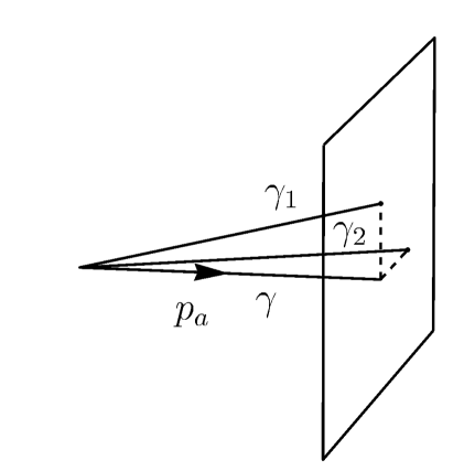
The reason why we are interested only in geodesics which lie on the same wavefront is that we want to study geodesics which cross at one point, either the emission point ${\cal S}$ or the observation point ${\cal O}$. If this is the case, then $\xi^{a}=0$ at either $\lambda_{\cal O}$ or $\lambda_{\cal S}$, so that (2.7) is trivially satisfied there and thus also everywhere on $\gamma$.

By imposing (2.6) and (2.7) we have effectively reduced the number of degrees of freedom from four to three. It turns out that a further reduction is possible. Note that at every point we are free to add a vector proportional to $p^{a}$ to both $\xi^{a}$ and $\nabla_{p}\xi^{a}$. The former corresponds to using a different point of the same geodesic $\gamma$ in the definition of the separation vector $\xi^{a}$, while the latter is just a rescaling of the affine parametrization of $\gamma$. Neither transformation affects the physical content of the equations, as long as we are in the regime of geometrical optics. As a matter of fact, it is easy to see that equations (2.5)–(2.7) are insensitive to these transformations as well:

$$\nabla_{p}\nabla_{p}\left(\xi^{a}+C(\lambda)\,p^{a}\right)=R^{a}_{\phantom{a}bcd}\,p^{b}\,p^{c}\,\xi^{d}+\ddot{C}\,p^{a}$$ (2.8)

$$\nabla_{p}\left(\xi^{a}+C(\lambda)\,p^{a}\right)\,p_{a}=\dot{C}\,p^{a}\,p_{a}=0$$ (2.9)

$$\left(\xi^{a}+C(\lambda)\,p^{a}\right)\,p_{a}=C\,p^{a}\,p_{a}=0.$$ (2.10)

It follows that (2.5)–(2.7) can be reinterpreted as equations on the space $p^{\perp}/p$, consisting of vectors orthogonal to $p_{a}$ and divided by the relation $\xi^{a}\sim\eta^{a}\iff\xi^{a}=\eta^{a}+A\,p^{a}$. We shall denote the equivalence class corresponding to a vector $\xi^{a}$ in $p^{\perp}$ as $\left[\xi\right]^{A}$. The space $p^{\perp}/p$ is two–dimensional and inherits the positive-definite metric from $g_{ab}$ via the relation $\left[X\right]^{A}\,\left[Y\right]^{B}\,g_{AB}=X^{a}\,Y^{b}\,g_{ab}$, where $X^{a}$ and $Y^{b}$ are any vectors in the tangent space corresponding to the equivalence classes $[X]^{A}$ and $[Y]^{B}$, respectively. It can be thought of as the space of null geodesics lying in the neighbourhood of $\gamma$ on the same wavefront, without any specification of which point on $\gamma$ we assign to which point of $\tilde{\gamma}$. It is straightforward to verify that the covariant derivative $\nabla_{p}$ can also be defined as an operator on $p^{\perp}/p$.

In the standard formalism due to Sachs [22, 23], we then introduce a frame with two spatial, orthonormal screen vectors $\xi_{1}^{a}$ and $\xi_{2}^{a}$, both orthogonal to $p^{a}$ and to a timelike observer $u^{a}_{\cal O}$. Notice that this is not strictly necessary: all that matters in geometrical optics are the equivalence classes $\left[\xi_{1}\right]^{A}$ and $\left[\xi_{2}\right]^{B}$, which turn out to be entirely $u^{a}_{\cal O}$-independent. More precisely, for any other choice of the observer $\tilde{u}^{a}_{\cal O}$ and the corresponding $\tilde{\xi}_{1}^{a}$ and $\tilde{\xi}_{2}^{a}$ perpendicular to $p_{a}$, the classes $\left[\tilde{\xi}_{1}\right]^{A}$ and $\left[\tilde{\xi}_{2}\right]^{B}$ are related to $\left[\xi_{1}\right]^{A}$ and $\left[\xi_{2}\right]^{B}$ via a simple spatial rotation.

The image distortion of a distant object and its angular distance can now be calculated by finding the Jacobi matrix ${\cal D}^{A}_{\phantom{A}B}$ of the GDE in the space $p^{\perp}/p$

$$\nabla_{p}\nabla_{p}{\cal D}^{A}_{\phantom{A}B}=R^{A}_{\phantom{A}\mu\nu C}\,p^{\mu}\,p^{\nu}\,{\cal D}^{C}_{\phantom{C}B}$$ (2.11)

with the initial data of the form

$${\cal D}^{A}_{\phantom{A}B}(\lambda_{\cal O})=0$$ (2.12)

$$\nabla_{p}{\cal D}^{A}_{\phantom{A}B}(\lambda_{\cal O})=\delta^{A}_{\phantom{A}B}$$

(see [23] for its geometric definition and the discussion of its properties). Note that the initial data depends on the choice of parametrization of the null geodesic $\gamma$, because if we rescale $\lambda\mapsto C\,\lambda$, the tangent vector rescales accordingly via $p^{a}\to C^{-1}p^{a}$. Thus ${\cal D}^{A}_{\phantom{A}B}$ is parametrization-dependent. Nevertheless, the tensor product $p_{\mu}\,{\cal D}^{A}_{\phantom{A}B}$ is parametrization-independent and is therefore an intrinsic property of the light cone centred at the observation point $\cal O$. In practice the equations (2.11)–(2.12) are solved by first introducing a Sachs frame and then using the corresponding screen vectors $\left[\xi_{1}\right]^{A}$ and $\left[\xi_{2}\right]^{B}$ as a basis in $p^{\perp}/p$.

The image distortion seen by the observer with 4-velocity $u_{\cal O}^{a}$ at the observation point is finally:

$$I^{A}_{\phantom{A}B}=\left|u_{\cal O}^{a}\,p_{a}\right|\,{\cal D}^{A}_{\phantom{A}B}(\lambda_{\cal S})$$ (2.13)

while the angular distance is

$$D_{\rm A}=\left|u_{\cal O}^{a}\,p_{a}\right|\,\sqrt{\left|\det{\cal D}^{A}_{\phantom{A}B}(\lambda_{\cal S})\right|}$$ (2.14)

(see also [23] and references therein). Note that the result does not depend on the 4-velocity of the source, while the dependence on the 4-velocity of the observer is quite simple. For instance, it is easy to prove that, on an FLRW spacetime, observers boosted with respect to the comoving frame measure smaller angular distances, because the quantity $\left|u_{\cal O}^{a}\,p_{a}\right|$ decreases as the boost parameter is increased. One can therefore use equation (2.14) to work out which observers (if any) would measure a specified angular distance for an object in a given spacetime.

The luminosity distance is defined using the total energy flux from the source through a fixed area at the observation point. In the formalism above it can be expressed as

$$D_{\rm L}=\left|u_{\cal S}^{a}\,p_{a}\right|\,\sqrt{\left|\det\tilde{\cal D}^{A}_{\phantom{A}B}(\lambda_{\cal O})\right|}(1+z)$$ (2.15)

where $\tilde{\cal D}^{A}_{\phantom{A}B}$ satisfies (2.11), but with the initial conditions (2.12) imposed at the source rather than at the observer, and $z$ is the relative change in the photon frequency as it moves along the geodesic, also known as its redshift:

$$z=\frac{\nu_{\cal S}-\nu_{\cal O}}{\nu_{\cal O}}=\frac{u_{\cal S}^{a}\,p_{a}}{u_{\cal O}^{a}\,p_{a}}-1.$$ (2.16)

The fundamental result by Etherington [24] relates these quantities: the reciprocity relation reads

$$\left|\det\tilde{\cal D}^{A}_{\phantom{A}B}(\lambda_{\cal O})\right|=\left|\det{\cal D}^{A}_{\phantom{A}B}(\lambda_{\cal S})\right|.$$ (2.17)

It follows easily that

$$D_{\rm L}=(1+z)^{2}D_{\rm A}.$$ (2.18)

Relation (2.17) allows one to calculate both distances by solving the GDE with the initial conditions (2.12) imposed either at the source or at the observation point.

In this paper we have found it much simpler to impose the initial conditions at the location of the source, and to integrate the equations forward in time. Moreover, instead of solving the GDE directly, we simply use the geodesic tracker and follow directly two additional null geodesics $\gamma_{1}(\lambda)$ and $\gamma_{2}(\lambda)$, slightly perturbed with respect to the principal one, which we denote with $\gamma_{0}(\lambda)$. We specify the initial conditions for them at the source:

$$x^{a}_{1}(\lambda_{\cal S}) = x^{a}_{2}(\lambda_{\cal S})=x^{a}_{0}(\lambda_{\cal S})$$ (2.19)

$$p_{1}^{a}(\lambda_{\cal S}) = p_{0}^{a}(\lambda_{\cal S})+\epsilon\xi_{1}^{a}(\lambda_{\cal S})$$ (2.20)

$$p_{2}^{a}(\lambda_{\cal S}) = p_{0}^{a}(\lambda_{\cal S})+\epsilon\xi_{2}^{a}(\lambda_{\cal S})$$ (2.21)

where $x^{a}_{I}$ are the coordinates of geodesic $\gamma_{I}$ and $p^{a}_{I}$ is its 4-momentum. We can then compute ${\cal D}^{A}_{\phantom{A}B}$ by using the fact that:

$${\cal D}^{A}_{\phantom{A}B}(\lambda) = \lim_{\epsilon\to 0}\frac{\sqrt{g(\lambda_{\cal S})}}{\epsilon}\left[\begin{array}[]{ll}g_{ab}(x^{a}_{1}-x^{a}_{0})\,\xi_{1}^{b}&g_{ab}(x^{a}_{2}-x^{a}_{0})\,\xi_{1}^{b}\\[14.22636pt] g_{ab}(x^{a}_{1}-x^{a}_{0})\,\xi_{2}^{b}&g_{ab}(x^{a}_{2}-x^{a}_{0})\,\xi_{2}^{b}\end{array}\right]$$ (2.24)

where $g(\lambda_{\cal S})$ is the determinant of $g_{ab}$ at the geodesic initial location. This is the approach we take in the computations described in Section 4.

2.1 Homogeneous cosmologies

This formalism takes on a particularly simple form in the exactly homogeneous and isotropic cosmological models (the FLRW class), defined by the line element:

$$ds^{2}=-dt^{2}+a(t)^{2}dl^{2}$$ (2.25)

where $dl^{2}$ is the line element of one of the three three-dimensional constant-curvature spaces of Euclidean signature. In this case, geodesics can move along coordinate lines and be parametrized by the coordinate time. In the flat case, for instance, we can choose $x$ as the geodesic direction (so that $\xi_{1}^{a}=a(t)\delta_{y}^{a}$ and $\xi_{2}^{a}=a(t)\delta_{z}^{a}$, where $a(t)$ is the scale factor). The matrix ${\cal D}^{A}_{\phantom{A}B}$ is then given by:

$${\cal D}^{A}_{\phantom{A}B}(t) = a_{\cal S}\left[\begin{array}[]{cc}a(t)x(t)&0\\ 0&a(t)x(t)\end{array}\right]$$ (2.28)

where $x(t)$ is the coordinate distance travelled along the geodesic at time $t$:

$$x(t)=\int_{t_{\cal S}}^{t}\frac{dt}{a(t)}$$ (2.29)

Given the initial normalization $u_{\cal S}^{a}\,p_{a}=-a_{\cal S}^{-1}$, equation (2.15) becomes:

$$D_{\rm L}=a_{\cal O}(1+z)\int_{t_{\cal S}}^{t_{\cal O}}\frac{dt}{a(t)}$$ (2.30)

Noticing that, in an FLRW model, the redshift $z$ only depends on the ratio between the scale factor at the time of detection and the scale factor at the time of emission:

$$z=\frac{a(t_{\cal O})}{a(t_{\cal S})}-1,$$ (2.31)

it is easy to show that equation (2.30) coincides with the usual textbook expression for $D_{\rm L}$, which we quickly recall. We first need to calculate the comoving distance covered by a photon between ${\cal S}$ and ${\cal O}$:

$$D_{\rm M}(z)=a_{\cal O}\int_{t_{\cal S}}^{t_{\cal O}}\frac{dt}{a(t)}=(1+z)S\left(\Omega_{k},\int_{0}^{z}\frac{d\zeta}{H(\zeta)(1+\zeta)^{2}}\right),$$ (2.32)

with

$$H(\zeta)=H_{\cal S}\sqrt{\Omega^{\cal S}_{\rm M}(1+\zeta)^{-3}+\Omega^{\cal S}_{\Lambda}+\Omega^{\cal S}_{k}(1+\zeta)^{-2}},$$ (2.33)

and

$$S(k,x) = \left\{\begin{array}[]{ll}k^{-1/2}\sin k^{1/2}x&\textrm{for }k>0\\ x&\textrm{for }k=0\\ |k|^{-1/2}\sinh|k|^{1/2}x&\textrm{for }k<0\end{array}\right.$$ (2.37)

Notice that the reference values for all quantities are those at the source: $a_{\cal S}$, $H_{\cal S}$, and $\Omega^{\cal S}_{\rm X}$ are the model’s scale factor, Hubble rate, and density parameters at the time the photon is emitted, respectively. As is customary, we also define the curvature $\Omega$ parameter by:

$$\Omega^{\cal S}_{k}=1-\Omega^{\cal S}_{\rm M}-\Omega^{\cal S}_{\Lambda}.$$ (2.38)

Notice that referring to the initial values of these parameters rather than the final ones changes our expressions from the standard textbook treatment. It is straightforward to show that the usual formulae are recovered if one expresses all quantities at the source in terms of the corresponding ones at the observer.

Having found an expression for $D_{\rm M}(z)$, we can use it to derive the apparent luminosity $\ell$ of an object of intrinsic luminosity ${\cal L}$ (for details, see e.g. [25]):

$$\ell=\frac{\cal L}{4\pi D_{\rm M}(z)^{2}(1+z)^{2}}.$$ (2.39)

Since the apparent luminosity is defined as:

$$D_{\rm L}(z)=\sqrt{\frac{\cal L}{4\pi\ell}},$$ (2.40)

we finally obtain:

$$D_{\rm L}(z)=D_{\rm M}(z)(1+z)=(1+z)^{2}S\left(\Omega_{k},\int_{0}^{z}\frac{d\zeta}{H(\zeta)(1+\zeta)^{2}}\right)$$ (2.41)

This can be easily identified, on a flat background, with (2.30). In homogeneous and isotropic cosmologies, therefore, the luminosity distance only depends on the redshift, and is parametrized by global quantities such as the matter density and the curvature of spatial slices. In the Einstein-de Sitter (EdS) model, $D_{\rm L}$ simply reduces to

$$D_{\rm L}(z)=\frac{2(1+z)^{2}}{H_{\cal S}}\left((1+z)^{1/2}-1\right)$$ (2.42)

2.2 Inhomogeneous cosmologies

The propagation of light in lumpy spacetimes has been studied since the 1960’s with various approaches, starting with the EBA proposed in [11] and later generalized in [12, 13]. The key idea inspiring these studies is that, in cosmological models where the matter is distributed in lumps, a large fraction of the light beams would not contain matter, and would therefore not be affected by the Ricci focusing characteristic of their FLRW counterparts.

Other limitations of the FLRW approximation and the related physical effects were subsequently analysed, both in approximate scenarios and in exact cosmological models (typically belonging to the Swiss-Cheese family) [16, 21, 26, 27, 28, 29, 30, 31, 32, 33, 34, 35, 36, 37, 38, 39]. A few robust features of these studies, that do not depend on the details of the models used, include that:

• Light sources appear reduced in size and dimmer in a lumpy spacetime than in a homogeneous one with the same mean density;

• The angular distance does not have a maximum, but keeps growing all the way to the cosmic horizon;

• The actual deceleration parameter $q_{0}$ is larger than in the case where the same data is analysed with an FLRW model with the same mean density.

Later, when we measure the $D_{\rm L}(z)$ relationship in BHL spacetimes, we will use these features as guidelines for what to expect. Many of them do indeed hold for such highly nonlinear spacetimes too.

In fact, as discussed at length in Section 4, the luminosity distance in a BHL follows rather closely the EBA [11], which we report for completeness:

$$D_{\rm L}(z)=\frac{2(1+z)^{2}}{5H_{\cal S}}\left(1-\frac{1}{(1+z)^{5/2}}\right).$$ (2.43)

In Section 3 we will explain why the EBA is a good approximation of the redshift–luminosity distance in a BHL, and point out that it is equivalent to neglecting the Ricci term in the standard geodesic deviation equation.

2.3 Geodesics and observer classes

As with many other quantities of interest that can be calculated in inhomogeneous cosmologies, the calculation of $D_{\rm L}(z)$ requires the choice of a time coordinate. In general, representing the spacetime in the geodesic gauge will lead to coordinate observers which are diversely affected by neighbouring gravitational structures, and may experience, e.g., light redshifting which has nothing to do with a global, suitably defined expansion rate (an observational cosmologist would call these local effects).

A study of light propagation in inhomogeneous spaces, especially one that is targeted at the comparison with the FLRW class, is then left with two possibilities: a statistical approach in which observers and sources are distributed stochastically throughout the spacetime, and a single $D_{\rm L}(z)$ relationship is obtained by averaging over their locations and four-momenta; or the construction of one or more classes of cosmological observers, based on geometry-inspired considerations such as following the geodesics of the average gravitational field, or geodesics with minimal deviation. We find the latter approach more likely to yield insight on the different gauge choices and related effects, and therefore use it in the remaining of this paper. Statistical reasoning is, however, also an important ingredient, as the observational data is arguably to be modelled through a mix of different observer and source states of motion. As statistical analyses are a tricky endeavour in cosmology, we leave this task for future work.

Notice that the second strategy is particularly difficult to deploy on vacuum spacetimes, as the sources of the gravitational field are only perceived through their effect on the metric tensor, and not through the presence of matter, so singling out a “local” component of the gravitational field will in some cases not even be well defined (for a discussion of this point, see e.g. [40] or [23] and references therein). We will however exploit the existence of global (albeit discrete) symmetries in our BHLs and only turn our attention to geodesics which are by construction least affected by local effects: these include, for instance, the geodesics running along the edges of the fundamental periodic cell constituting the lattice.

3 Light propagation in BHLs

In this section, we build an approximate model for the propagation of light in a BHL, based on a perturbative expansion in the BHL compactness parameter. This will serve as a qualitative analysis of the physics of the propagation of light and as a support in the interpretation of the numerical results presented in section 4. Note that an expansion in a similar parameter has already appeared in the context of BHLs [20], although the details are different.

3.1 A perturbative expansion in the compactness parameter

Let $L$ denote the characteristic size of a lattice cell, such as its initial geodesic length, and let $M$ be a characteristic mass, i.e. the total mass contained in a cell. As in [4], we can introduce the dimensionless parameter

$$\mu=\frac{M}{L}$$ (3.1)

measuring the lattice compactness. If we additionally introduce the characteristic mass density $\rho=ML^{-3}$, we can see that

$$\mu=\rho L^{2},$$ (3.2)

i.e. it goes down to zero as we decrease the size of a cell keeping the mass density of the corresponding FLRW model fixed. Note that $\rho$ is related to the curvature scale of the Friedmann model via $R=\rho^{-1/2}$, so $\mu$ can be reinterpreted as the separation of scales between the size of an individual lattice cell and the radius of curvature of the FLRW model:

$$\mu=\frac{L^{2}}{R^{2}}.$$ (3.3)

Note that the definition of $\mu$ involves a certain vagueness: we may take for the mass scale $M$ the ADM mass of the black hole measured at the other end of the Einstein-Rosen bridge, but also some other related parameter. Also the choice of the length scale involves a certain arbitrariness. At the leading order we expect this ambiguity to be irrelevant.

We will now show how $\mu$ can be used to find a perturbative approximation for the metric tensor of the lattice model. The approximation is different from the standard perturbative approximation on an FLRW background, in the sense that it does not require the density contrast $\delta$ of the matter perturbation to be small. Obviously the problem of BHLs lies beyond the validity regime of the cosmological perturbation theory, because in a BHL we are dealing with $\delta=-1$ everywhere.

We begin by introducing a coordinate system on a single cell. Let $g^{(0)}$ denote the background FLRW metric and $x^{\mu}$ be the Riemannian normal coordinate system around any point $P$. The metric takes the form of

$$g^{(0)}_{\mu\nu}=\eta_{\mu\nu}-\frac{1}{3}R_{\mu\alpha\nu\beta}\Big{|}_{P}\,x^{\alpha}\,x^{\beta}+O(x^{3}).$$ (3.4)

Since $R$ is the curvature scale of the metric, the coefficients in the expansion above are of order $R^{0}$ (the flat metric), $R^{-2}$ (the Riemann tensor), $R^{-3}$ (the next term involving $\nabla_{\sigma}R_{\mu\alpha\nu\beta}$), and so on. The Taylor expansion in the Riemannian normal coordinates becomes thus the expansion in negative powers of $R$. We now introduce the rescaled coordinates $\tilde{x}^{\mu}=L^{-1}\,x^{\mu}$ and the rescaled Riemann tensor at point $P$ in coordinates $x^{\mu}$.

$$r_{\mu\alpha\nu\beta}=R^{2}\,R_{\mu\alpha\nu\beta}\Big{|}_{P}.$$ (3.5)

Both $\tilde{x}$ and $r_{\mu\alpha\nu\beta}$ are $O(1)$ in the expansion in $R$, at least within a single lattice cell around $P$. The metric $g^{(0)}$ can be expressed in the new coordinates. The metric tensor components in those coordinates will be denoted by ${\tilde{g}}^{(0)}_{\mu\nu}$, i.e.

$$g^{(0)}=g^{(0)}_{\mu\nu}\,\textrm{d}x^{\mu}\otimes\textrm{d}x^{\nu}={\tilde{g}}^{(0)}_{\mu\nu}\,\textrm{d}\tilde{x}^{\mu}\otimes\textrm{d}\tilde{x}^{\nu}.$$ (3.6)

Its expansion in $\tilde{x}^{\mu}$ takes the form of

$${\tilde{g}}^{(0)}_{\mu\nu}=L^{2}\left(\eta_{\mu\nu}-\frac{\mu}{3}r_{\mu\alpha\nu\beta}\,\tilde{x}^{\alpha}\,\tilde{x}^{\beta}+O(\tilde{x}^{3}L^{3})\right).$$ (3.7)

The first of the remaining higher-order terms $\nabla_{\sigma}R_{\mu\alpha\nu\beta}\,L^{3}\,\tilde{x}^{\sigma}\,\tilde{x}^{\alpha}\,\tilde{x}^{\beta}$ contains the covariant derivative $\nabla_{\sigma}R_{\mu\alpha\nu\beta}\Big{|}_{P}$, which is $O(R^{-3})$ as we noted before. Therefore the whole term in question can be re-expressed as $r_{\sigma\mu\alpha\nu\beta}\,\tilde{x}^{\sigma}\,\tilde{x}^{\alpha}\,\tilde{x}^{\beta}\,\frac{L^{3}}{R^{3}}$, where we have defined by analogy the rescaled derivative of the curvature $r_{\sigma\mu\alpha\nu\beta}=R^{3}\,\nabla_{\sigma}R_{\mu\alpha\nu\beta}$, which again is $O(1)$ in $R$. We see that the whole term turns out to be $O(\mu^{3/2})$. Similar reasoning can be applied to all higher terms, yielding higher powers of the dimensionless parameter $\mu$. We thus see that

$${\tilde{g}}^{(0)}_{\mu\nu}=L^{2}\left(\eta_{\mu\nu}-\frac{\mu}{3}r_{\mu\alpha\nu\beta}\,\tilde{x}^{\alpha}\,\tilde{x}^{\beta}+O(\mu^{3/2})\right),$$ (3.8)

i.e. in the rescaled coordinates the expansion in the negative powers of $R$ turns in a natural way into an expansion in powers of $\mu$, valid in a region of size $L$ around $P$.

We can explain the physical meaning of the expansion above in the following way: if the background metric $g^{(0)}$ has the curvature scale of $R$, then in an appropriately picked, quasi-Cartesian coordinate system $x^{\mu}$ it has the Taylor expansion in which the terms are of increasing order in $R^{-1}$. If we then pick a domain of size $L$, then the metric in this domain, again in appropriate coordinates, has the form of the flat metric plus perturbations from the curvature and its derivatives. A simple way to obtain a perturbation of this kind is to use the Taylor expansion we mentioned before and rescale the coordinates by $L$, which yields an expansion in powers of $\mu^{1/2}$.

Now we can add the perturbation due to the discrete matter content. We assume the full metric to be

$$\tilde{g}_{\mu\nu}=L^{2}\left(\eta_{\mu\nu}-\frac{\mu}{3}r_{\mu\alpha\nu\beta}\,\tilde{x}^{\alpha}\,\tilde{x}^{\beta}+\mu\,h_{\mu\nu}\left(\tilde{x}^{\alpha}\right)+O(\mu^{3/2})\right)$$ (3.9)

with the perturbation $h_{\mu\nu}\left(\tilde{x}^{\alpha}\right)$ of order $O(1)$ in $\mu$. Note that the dependence on $\tilde{x}^{\mu}$ means that the characteristic physical size of the perturbation is the size of a cell, i.e. $L$. The Einstein tensor of the metric above is

$$G_{\mu\nu}\left[\tilde{g}_{\alpha\beta}\right]=G_{\mu\nu}\left[{\tilde{g}}^{(0)}_{\alpha\beta}\right]+\mu\,G^{\prime}_{\mu\nu}\left[h_{\alpha\beta}\right]\left(\tilde{x}^{\alpha}\right)+O(\mu^{3/2}),$$ (3.10)

where $G^{\prime}_{\mu\nu}[\cdot]$ is the linearisation of the Einstein tensor around a flat metric $\eta_{\mu\nu}$. In particular, in the harmonic gauge it is simply $-\frac{1}{2}\Box h_{\alpha\beta}$. We now return to the original, unrescaled coordinate system, where this equation takes the form of

$$G_{\mu\nu}\left[g_{\alpha\beta}\right]=G_{\mu\nu}\left[g^{(0)}_{\alpha\beta}\right]+\rho\,G^{\prime}_{\mu\nu}\left[h_{\alpha\beta}\right]\left(x^{\alpha}/L\right)+O(\mu^{3/2}),$$ (3.11)

i.e. the perturbation of the Einstein tensor is $O(\rho)$, just like the Einstein tensor of the FLRW metric. It means that this approximation works even if the density perturbation is of the order of the background energy density. We may therefore use $h_{\mu\nu}$ to cancel the stress-energy tensor of the underlying FLRW metric everywhere except on a single worldline.

Recall that $G_{\mu\nu}\left[g^{(0)}_{\alpha\beta}\right]=8\pi G\rho\,u_{\mu}u_{\nu}$, where $u^{\mu}=(1,0,0,0)$ is the cosmic fluid 4-velocity. We impose the linear PDE on the metric perturbation:

$$G^{\prime}_{\mu\nu}\left[h_{\alpha\beta}\right]=8\pi G\left(-1+C\delta^{(3)}(x^{\alpha})\right)u_{\mu}\,u_{\nu}$$ (3.12)

with periodic boundary conditions and with the constant $C$ chosen so that the RHS integrates out to zero over one cell. The solution can be obtained using Appell’s $\zeta$ function [41]. It diverges at the centre, where the approximation fails, but near the cell’s boundary it is likely to work well. The resulting approximate metric is vacuum everywhere and periodic.

3.2 The continuum limit

Let us now consider the metric (3.9) along with its Christoffel symbols and Riemann tensor. It is straightforward to see that

$$\tilde{g}_{\mu\nu} = {\tilde{g}}^{(0)}_{\mu\nu}+L^{2}\,\mu\,h_{\mu\nu}(\tilde{x}^{\rho})$$ (3.13)

$$\Gamma^{\alpha}_{\phantom{\alpha}\beta\gamma}\left[\tilde{g}_{\kappa\lambda}\right] = \Gamma^{\alpha}_{\phantom{\alpha}\beta\gamma}\left[{\tilde{g}}^{(0)}_{\kappa\lambda}\right]+\mu\,{\Gamma^{\prime}}^{\alpha}_{\phantom{\alpha}\beta\gamma}\left[h_{\kappa\lambda}\right](\tilde{x}^{\rho})$$ (3.14)

$$R^{\alpha}_{\phantom{\alpha}\beta\gamma\delta}\left[\tilde{g}_{\kappa\lambda}\right] = R^{\alpha}_{\phantom{\alpha}\beta\gamma\delta}\left[{\tilde{g}}^{(0)}_{\kappa\lambda}\right]+\mu\,{R^{\prime}}^{\alpha}_{\phantom{\alpha}\beta\gamma\delta}\left[h_{\kappa\lambda}\right](\tilde{x}^{\rho}).$$ (3.15)

We can now go back to the original, unrescaled coordinates and obtain

$$g_{\mu\nu} = g^{(0)}_{\mu\nu}+\mu\,h_{\mu\nu}\left(x^{\rho}/L\right)$$ (3.16)

$$\Gamma^{\alpha}_{\phantom{\alpha}\beta\gamma}\left[g_{\kappa\lambda}\right] = \Gamma^{\alpha}_{\phantom{\alpha}\beta\gamma}\left[g^{(0)}_{\kappa\lambda}\right]+\mu^{1/2}\,\rho^{1/2}\,{\Gamma^{\prime}}^{\alpha}_{\phantom{\alpha}\beta\gamma}\left[h_{\kappa\lambda}\right]\left(x^{\rho}/L\right)$$ (3.17)

$$R^{\alpha}_{\phantom{\alpha}\beta\gamma\delta}\left[g_{\kappa\lambda}\right] = R^{\alpha}_{\phantom{\alpha}\beta\gamma\delta}\left[g^{(0)}_{\kappa\lambda}\right]+\rho\,{R^{\prime}}^{\alpha}_{\phantom{\alpha}\beta\gamma\delta}\left[h_{\kappa\lambda}\right]\left(x^{\rho}/L\right)$$ (3.18)

plus higher order terms in $\mu$. Consider now the limit $\mu\to 0$, i.e. where the size of the perturbations decreases in comparison to the curvature scale of the background FLRW model, or the limit where the compactness $M/L$ vanishes. Obviously we see that the metric tensor and the Christoffel symbols converge to the FLRW values in this case, while the curvature does not. This is due to the fact that the metric $g_{\mu\nu}$ is that of a vacuum spacetime for all positive $\mu$, while the FLRW one is not. This is a key observation in the study of the optical properties of a BHL, which are determined by the GDE and are therefore sensitive to the form of the Riemann tensor.

To illustrate this point, consider first a null geodesic. It follows from equations (3.16)–(3.18) above that its equation has the form of a perturbed FLRW geodesic

$$x^{\mu}(\lambda)=\tilde{x}^{\mu}(\lambda)+\mu^{1/2}\,\delta x^{\mu}(\lambda).$$ (3.19)

where the tilde denotes the FLRW solution without the inhomogeneities. The parallel transport of a frame along the geodesic has a similar expansion in $\mu$:

$$e_{a}^{\phantom{a}\mu}(\lambda)=\tilde{e}_{a}^{\phantom{a}\mu}(\lambda)+\mu^{1/2}\,\delta e_{a}^{\phantom{a}\mu}(\lambda).$$ (3.20)

We can now rewrite the GDE in the parallel-propagated frame along the geodesic

$$\frac{\textrm{d}^{2}X^{a}}{\textrm{d}\lambda^{2}} = \left(R^{a}_{\phantom{a}bcd}\left[g^{(0)}_{\kappa\lambda}\right]+\rho\,{R^{\prime}}^{a}_{\phantom{a}bcd}\left[h_{\kappa\lambda}\right]\right)p^{b}\,p^{c}+O(\mu^{1/2}).$$ (3.21)

We see that, already at the leading order $O(1)$ in $\mu$, we must take into account the full physical Riemann tensor instead of the simple FLRW one. In particular, since the BHLs are vacuum spacetimes, we need to solve the Ricci-free GDE and possibly take into account the non-vanishing Weyl tensor along the way in order to calculate the angular and luminosity distance. Neglecting the Ricci tensor in the GDE is equivalent to the EBA (for a discussion of this point, see e.g. [16]). We may thus expect the redshift–luminosity relations for BHLs in the continuum limit to be close to the EBA.

At the $O(\mu^{1/2})$ order we may expect additional corrections to $D_{\rm L}$ and $D_{\rm A}$ due to higher-order contributions to the geodesic equation as well as to the GDE equation. Additionally, at this order we need to take into account the impact of the inhomogeneities on the observers in their free fall. In this work, we will not concern ourselves with a quantitative analysis of these effects, but we will signal their appearance to the reader when appropriate.

4 Results

In order to compute the relationship between redshift and luminosity distance on the spacetime of an expanding BHL, we carry out the numerical integration of the geodesic equation (with null tangent), along with the integration of Einstein’s equation required to obtain the metric tensor. The latter operation is performed by a code generated with the Einstein Toolkit, based on the Cactus [42] software framework along with modules such as Carpet [43, 44], McLachlan [45, 46], and CT_MultiLevel [47], as already presented in [2, 4, 8]. The geodesic integrator, on the other hand, is a new Cactus module that we have written. It implements a 3+1 decomposition of the geodesic equation in the form given in [48] and we have verified it against several exact solutions, as reported in Appendix B.

4.1 Initial data and evolution

As in [1, 4] we first construct an initial-data configuration by solving the Hamiltonian and momentum constraints on the cube $[-L/2,L/2]^{3}$ with periodic boundary conditions. In particular, we choose free data corresponding to conformal flatness:

$$\gamma_{ij}=\psi^{4}\delta_{ij}$$ (4.1)

and set the trace of the extrinsic curvature to zero around the origin and to a negative constant $K_{c}$ near the boundaries, with a transition region starting at a distance $l$ from the origin:

$$K_{ij} = \frac{1}{3}K_{\rm c}T(r)\gamma_{ij}+\psi^{-2}\tilde{A}_{ij}$$ (4.2)

$$T(r) = \left\{\begin{array}[]{ll}0&\textrm{for }0\leq r\leq l\\ \left(\frac{(r-l-\sigma)^{6}}{\sigma^{6}}-1\right)^{6}&\textrm{for }l\leq r\leq l+\sigma\\ 1&\textrm{for }l+\sigma\leq r\end{array}\right.$$ (4.6)

where we choose $l=0.05L$ and $\sigma=0.4L$. We represent the traceless part of the extrinsic curvature as:

$$\tilde{A}_{ij}=\tilde{D}_{i}X_{j}+\tilde{D}_{j}X_{i}-\frac{2}{3}\tilde{\gamma}_{ij}\tilde{D}_{k}X^{k}$$ (4.7)

and the conformal factor as:

$$\psi=\psi_{\rm r}+\frac{M}{2r}(1-T(r)),$$ (4.8)

where $M$ is the bare mass of the central black hole, and solve the constraints for $\psi_{\rm r}$ and $X^{i}$. For our basic configuration, we use $L=10$ and $M=1$ as in [4].

We then proceed to the time evolution of $\gamma_{ij}$ and $K_{ij}$ using a variant of the BSSN formulation, implemented in the McLachlan module, and to the concurrent integration of the geodesic equation (2.3).

4.2 Computation of geodesics

In order to compute geodesics in a 3+1 numerical spacetime, we first perform a 3+1 decomposition of the geodesic equation (2.3),

$${\nabla_{p}}p^{a}=0.$$ (4.9)

We decompose the geodesic tangent vector $p^{a}$ into its components along and orthogonal to the unit hypersurface normal $n^{a}$, which we call $\sigma$ and $q^{a}$, respectively: $p^{a}=\sigma n^{a}+q^{a}$. The vector $q^{a}$ is spatial, i.e. $q^{a}n_{a}=0$, and $\sigma=-n_{a}p^{a}$. We use an affine parametrisation, and $p^{a}$ is normalized as

$$p^{a}p_{a}=\kappa,$$ (4.10)

with $\kappa=0$ for null geodesics. The spatial coordinates, covariant components of the tangent vector and affine parameter of the geodesic, ($x^{i}$, $q_{i}$, $\lambda$) satisfy

$$\frac{dx^{i}}{dt} = -\beta^{i}+(p^{0})^{-1}\gamma^{ik}q_{k},$$ (4.11)

$$\frac{dq_{i}}{dt} = -p^{0}\alpha\alpha_{,i}+q^{j}\beta^{k}_{,i}\gamma_{kj}-\frac{1}{2}(p^{0})^{-1}q_{l}q_{m}\gamma^{lm}_{,i},$$ (4.12)

$$\frac{d\lambda}{dt} = (p^{0})^{-1}$$ (4.13)

where

$$p^{0} = \frac{(q_{k}q_{j}\gamma^{kj}-\kappa)^{1/2}}{\alpha}$$ (4.14)

is the time component of $p$ in the foliation-adapted coordinate basis. Note that the derivative is with respect to coordinate time $t$, not the affine parameter $\lambda$. These equations are the same as those given in [48], and a derivation is outlined in Appendix A.

Given $(x^{i},q_{i},\lambda)$ at a time $t$, equations (4.11)–(4.13) determine their evolution along a single geodesic. The right hand sides of eqs. (4.11)–(4.13) are computed by interpolating the metric quantities $\beta^{i}$, $\gamma_{ij}$, $\alpha$ from the evolution grid to the point $x^{i}(t)$ using fourth-order Lagrange interpolation, and $(x^{i}(t),q_{i}(t),\lambda(t))$ is integrated using a fourth-order Runge-Kutta method using the Cactus MoL component. Additionally, the metric and various other quantities of interest are interpolated to $x^{i}$, and all quantities are output as curves parametrised by $t$ for use in any subsequent analysis once the simulation is complete.

We implement the above prescription in two new Cactus components Geodesic and ParticleUtils. The former contains the equations themselves, and the latter provides library-type functionality for integrating systems of equations along curves. A few validation tests are provided in Appendix B.

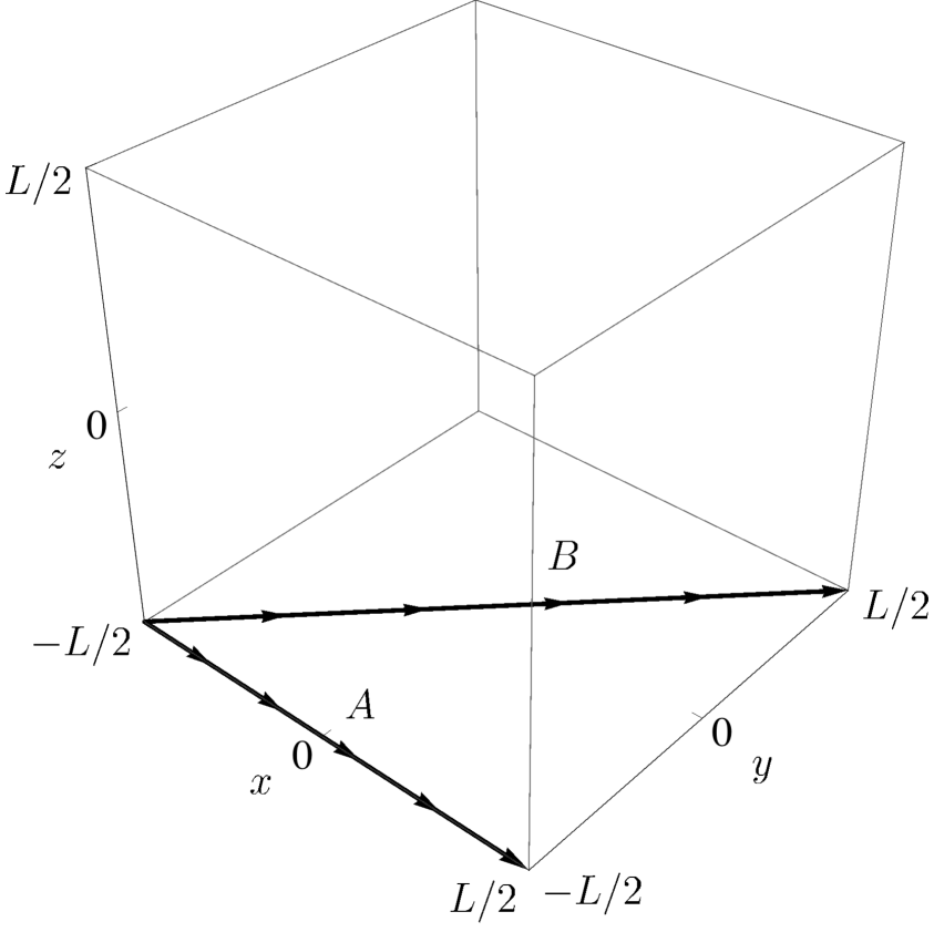
We now face the crucial task of selecting which geodesics to track. Let us notice that, on a space filled with periodic cells, symmetry reasons imply that an obvious class of cosmological observers is that formed by observers sitting at the cell vertices. Due to the symmetry, these observers do not exhibit any proper motions on top of the cosmic expansion, and the ratio of the proper distances between arbitrary pairs of observers is constant at all times. For this study, we construct and analyse two geodesics from this class (which we will denote $A$ and $B$), starting at the vertex $(-L/2,-L/2,-L/2)$, with initial tangents equal to $p_{a}^{A}=(p_{0}^{A},1,0,0)$ and $p_{a}^{B}=(p_{0}^{B},1/\sqrt{2},1/\sqrt{2},0)$ respectively. $p_{0}^{A}=-\alpha\sqrt{\gamma^{xx}}|_{A}$ and $p^{0}_{B}=-\alpha\sqrt{(\gamma^{xx}+\gamma^{yy}+2\gamma^{xy})/2}|_{B}$ are chosen by the geodesic integrator to ensure that the geodesics are null. The two geodesics are plotted in Figure 2.

In order to measure the luminosity distance along geodesics $A$ and $B$, we evolve two further pairs of geodesics, with spatial directions given by:

$$(1,\epsilon,0)$$ (4.15)

$$(1,0,\epsilon)$$ (4.16)

and

$$\left(\frac{1-\epsilon}{\sqrt{2}},\frac{1+\epsilon}{\sqrt{2}},0\right)$$ (4.17)

$$\left(\frac{1}{\sqrt{2}},\frac{1}{\sqrt{2}},\epsilon\right)$$ (4.18)

with $\epsilon=10^{-3}$, representative of two narrow beams close to each original geodesic. We can then construct the redshift and luminosity distance along the two beams. Again, we emphasize that, since we keep the source parameters fixed and observe the time evolution of each geodesic, this setup is different (but essentially equivalent) to the one usually adopted in cosmology, where the observer is fixed and sources with different parameters are considered.

As in [4], we run this configuration on a uniform grid with three different resolutions (corresponding to $160$, $256$, and $320$ points per side) in order to estimate the numerical error. All results presented below are convergent to first order, consistently with the convergence order reported for the geometric variables in [4]. All curves represent the Richardson extrapolation, at this order, of the numerical data. The corresponding truncation error (when visible) is indicated by a shaded region around each curve.

4.3 Small-redshift behaviour

For small distances $d$ from the source, we expect the photon redshift and luminosity distance to behave respectively like

$$z(d) \sim H_{\cal S}d$$ (4.19)

$$D_{\rm L}(d) \sim d$$ (4.20)

where $H_{\cal S}$ is related to the first time derivative of the local volume element at the source location:

$$H_{\cal S}=\left.\frac{{\rm tr}(K_{ij})}{3}\right|_{\cal S}$$ (4.21)

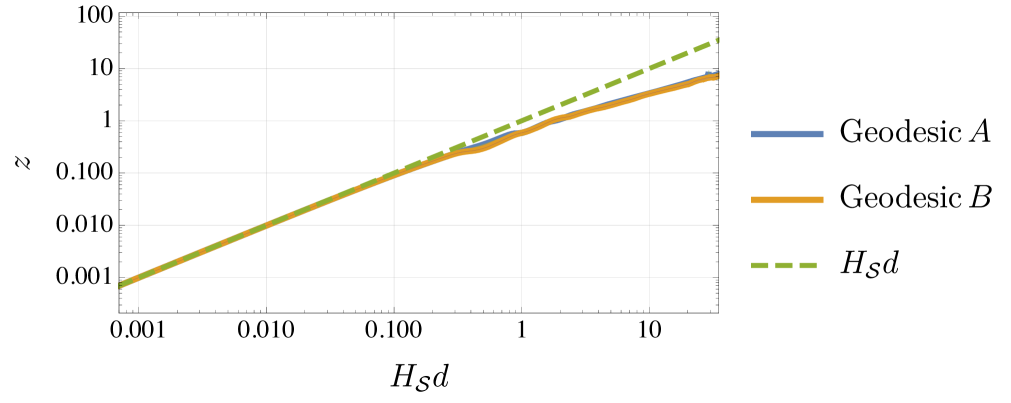
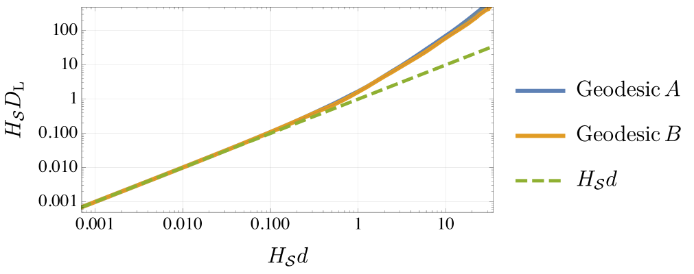
(see [26]). Figure 2 shows that this expectation is confirmed by our computation. For large $d$, however, both quantities grow larger than the linear order. Furthermore, the redshift clearly exhibits a non-monotonic behaviour engendered by the inhomogeneous gravitational field. This is easy to explain as a small, periodic redshift due to the photons climbing a potential hill near the vertices (away from the nearest black holes) and falling into wells near the edge or diagonal midpoints (closer to the black holes). Naturally, the two geodesics are affected in different ways as they trace different paths through the gravitational field.

Figure 2: Top: the paths of geodesics $A$ and $B$ in one of the BHL cells. The geodesics run close to the cell edge and diagonal, respectively, at all times. Middle: photon redshift as a function of the coordinate distance from the source. Bottom: luminosity distance as a function of the coordinate distance from the source. The error bars are indicated by shaded regions (when not visible, they are included in the width of the curves).

4.4 Luminosity distance

Due to numerical error, the geodesics deviate from the cell edge and face diagonal during the evolution, but remain quite close to them (the coordinate separation is less than $0.01\%$ after three cell crossings, in both cases). We can compare the $D_{\rm L}(z)$ relationship for geodesics $A$ and $B$ to the same quantity calculated according to four reference models:

1. The EdS model (equation (2.42));

2. An FLRW model (equation (2.41)) with $\Omega_{M}=0.3$ and $\Omega_{\Lambda}=0.7$ (henceforth denoted $\Lambda$CDM);

3. The Milne model [49], where redshift and luminosity distance are related by:

   $$D_{\rm L}(z)=\frac{1}{H_{\cal S}}\frac{z}{(1+z)^{2}}\left(1+\frac{z}{2}\right);$$ (4.22)

4. The estimate of $D(z)$ via the EBA, equation (2.43).

All models are fitted according to two prescriptions: the initial scale factor $a_{\cal S}$ is always set according to

$$a_{\cal S}={\rm det}(\gamma_{ij})^{1/6}|_{\cal S},$$ (4.23)

while the initial expansion rate $H_{\cal S}$ is set to either (i) the initial time derivative of the proper length of the domain edge (say, the one between $(-L/2,0,0)$ and $(L/2,0,0$)), which we call a global fit, and is the same procedure as [4]; or (ii) equation (4.21) (which we call a local fit).

Figure 3: Luminosity distance as a function of redshift for geodesics $A$ and $B$ (top plot). The same relationships in the EdS model, in the $\Lambda$CDM (i.e., FLRW with $\Omega_{\Lambda}=0.7$ and $\Omega_{M}=0.3$) model, in the Milne model and in the EBA are also plotted. The four models are fitted according to the procedure described in [4], using the global expansion rate computed from the first time derivative of the edge proper length. The relative difference between the four models and the BHL $D_{\rm L}$ is plotted in the second and third panel. The fourth and fifth panel illustrate the result of the same procedure, where the four models have been fitted using the local expansion rate (4.21) instead. On all plots, the dashed vertical lines mark the points where the geodesics cross over the periodic boundary. The error bars are indicated by shaded regions (when not visible, they are included in the width of the curves or of the data points).

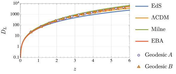
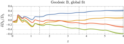
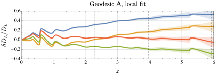
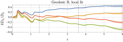
Figure 3 shows all the resulting curves. We first recall that the expansion of the BHL, measured by the proper distance of one of its cell edges, could be fitted quite well by an EdS model with the same initial expasion, as shown in [4]. The two models, however, exhibits markedly different optical properties. For geodesic $A$, the relative difference reaches $60\%$ by redshift $z=6$. This is not surprising: the conditions under which these light rays propagate in a BHL and in an EdS model are substantially different. In the former case, for instance, null geodesics infinitesimally close to $A$ or $B$ accelerate away from, rather than towards, them.

We notice that the EBA provides the best estimate for $D_{\rm L}(z)$ in a BHL. We conjecture that this result is due to the fact that this approximation can capture both the large-scale geometrical properties of a non-empty universe and the small-scale behaviour of light rays in vacuum. None of the other models satisfies both these conditions. Note also that, for longer times, the EBA works better for the geodesic $A$ (along the edge) than for geodesic $B$ (along the face diagonal). This is easy to explain if we notice that, because of the 4-fold discrete rotational symmetry around the edge, there are no Weyl focusing effects on $A$ and therefore the GDE with the Ricci tensor neglected and no Weyl contribution is likely to be a good approximation for the propagation of the neighbouring light rays. On the other hand along the face diagonal we may expect a non-vanishing Weyl lensing around the midpoint area due to the tidal distortion of the rays. Such an effect is not taken into account in the EBA.

4.5 Fitting the FLRW class

It is tempting to consider an FLRW cosmology with the same matter content and initial expansion as the reference EdS, plus an additional stress-energy contribution coming from a cosmological constant, and attempt to tune its value to reproduce the luminosity distance in the BHL.

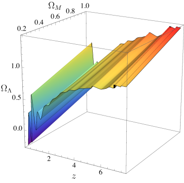
The left panel of Figure 4 shows a plot of the required $\Omega_{\Lambda}$ at each $z$, for values of $\Omega_{M}$ in $[0.2,1]$. The right panel shows a cross section of this surface with the planes $\Omega_{M}=1$ and $\Omega_{M}^{\rm eff}=8\pi/(3H_{\cal S}^{2}L_{\rm prop}^{3})$, where $L_{\rm prop}$ is the initial proper length of a cell edge. Notice, however, that none of these models would reproduce the expansion history of the BHL spacetime, which follows closely that of a region of an EdS model ($\Omega_{M}=1$ and $\Omega_{\Lambda}=0$) with the same $L_{\rm prop}$ and $H_{\cal S}$, as discussed in [4]. This is the core of the fitting problem: the mapping between different properties of an inhomogeneous spacetime to the FLRW class will be different, and in general it will not be possible to identify a single FLRW counterpart capable of reproducing all of the dynamical and optical aspects of an inhomogeneous cosmology.

Figure 4: Value of $\Omega_{\Lambda}$ in the best-fit FLRW cosmology, based on the luminosity distance measured on geodesic $A$ (left), and its cross sections with the planes $\Omega_{M}=1$ and $\Omega_{M}=\Omega_{M}^{\rm eff}=8\pi/(3H_{\cal S}^{2}L_{\rm prop}^{3})$ (curve yellow and blue, respectively, on the right plot). The error bars are indicated by shaded regions (when not visible, they are included in the width of the curves).

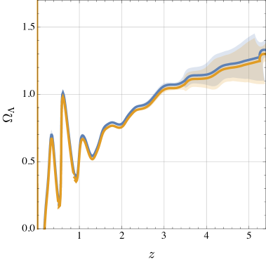
In Figure 5, we show the constant-$\Omega_{\Lambda}$ models which best fit the $D_{\rm L}(z)$ curves for geodesics $A$ and $B$. They are obtained for $\Omega_{\Lambda}^{A}=1.225$ and $\Omega_{\Lambda}^{B}=1.103$, respectively. The relative difference between these models and the exact solution is largest around $z=1$, where it reaches $30\%$.

Figure 5: $D_{\rm L}(z)$ for an FLRW model with $\Omega_{\rm M}=1$, and $\Omega_{\Lambda}$ equal to the best-fit values $\Omega_{\Lambda}^{A}=1.225$ and $\Omega_{\Lambda}^{B}=1.103$, as well as to a few other representative values. The best-fit models differ from the BHL $D_{\rm L}(z)$ at the $20\%$ level. The error bars are indicated by shaded regions (when not visible, they are included in the width of the curves or of the data points).

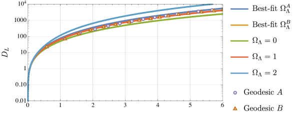
Notice that essentially all quantities discussed so far are affected by oscillations with a substantial initial amplitude, which is subsequently damped. Similarly to the oscillations in the redshift, we conjecture that these features are due to the inhomogeneous gravitational field, and in particular to radiative modes which likely originate in the oversimplified initial-data setup we employed. In a space without an asymptotically-flat region, it is of course difficult to test (or even formulate) this conjecture rigorously. The compactness of the spatial hypersurfaces, furthermore, means that one cannot simply ignore this initial transient as is customary in, e.g., binary-black-hole simulations, as the waves cannot escape from the domain (although their amplitude is significantly attenuated by the expansion). The presence of this unphysical component of the gravitational field, which we could barely notice in the length scaling we measured [4], affects very prominently, on the other hand, the BHL optical properties, and in particular the photon redshift. Better initial-data constructions which are free from these modes are an interesting field of investigation which goes beyond the purpose of this work.

Finally, it is worth observing that, as mentioned in Section 2, different observers would measure a different luminosity distance on the same spacetime, thereby potentially bringing the BHL result closer to the EdS curve. A boost with respect to the lattice would, for instance, lower the value of the distance, according to equation (2.14). So would a stronger gravitational field, as would be the case if an observer was located closer to the centre of a lattice cell.

4.6 Continuum limit $\mu\to 0$

Finally, it is instructive to study how this behaviour depends on how tightly packed the BHL is, as represented by the quantity $\mu=M/L$ introduced in Section 3. For simplicity, here we use the bare mass of the central black hole as an estimate of $M$, and the coordinate size of a cell edge as $L$. In order to keep $M/L^{3}$ constant at the value of our base configuration (which had $M=1$ and $L=10$), we need to have $\mu=M^{2/3}/10$. As representative masses we choose $M=\{1/100,1/8,1/2,1,5\}$; various properties of this BH family are illustrated in Table 1.

Table 1: The bare mass $M$, coordinate size of a cell edge $L=10M^{1/3}$, its proper size $L_{\rm prop}$, and the compactness parameter $\mu=M^{2/3}/10$ for a constant-density family of BHLs.

$M$	$L$	$L_{\rm prop}$	$\mu$
0.010	02.15	02.73	0.0046
0.125	05.00	06.28	0.0250
0.500	07.94	09.84	0.0630
1.000	10.00	12.26	0.1000
5.000	17.10	21.77	0.2924

We plot the luminosity distance as a function of $\mu$ in Figures 6 and 7. We observe, in particular, that the difference between the luminosity distance in a BHL and in an appropriately fitted EdS does not tend to zero as $\mu\to 0$. The EdS model, therefore, can reproduce the large-scale expansion history of a BHL (as illustrated numerically in [3, 4], and deduced analytically in [9]), but is unable to fit its optical properties, even in the limit $\mu\to 0$.

The numerical result is in agreement with the result of the perturbative analysis of Section 3, where we identified $O(1)$ differences in the GDE of a BHL with respect to that of an FLRW model. This indicates that cosmological-distance estimates of a lumpy spacetime based on a fit with the FLRW class will exhibit a systematic error, regardless of how lumpy the spacetime is. These effects are substantially, but not exhaustively, captured by the EBA, as already observed in the case of other inhomogeneous spacetimes [34, 35, 16].

Figure 6: Left: luminosity distance for a family of BHLs with the same density but varying $\mu$. Right: residual with respect to the EdS model (fitted via the local expansion rate) of the four lowest-mass models along with their extrapolation for $\mu\to 0$.

Figure 7: Behaviour of the luminosity distance at fixed redshift, for various values of $\mu$. The green triangle represents the polynomial extrapolation of the data series for $\mu\to 0$, while the yellow dashed curve represents the expected luminosity distance in EdS for each specific value of $z$.

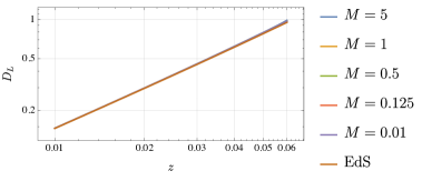
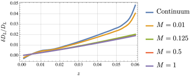
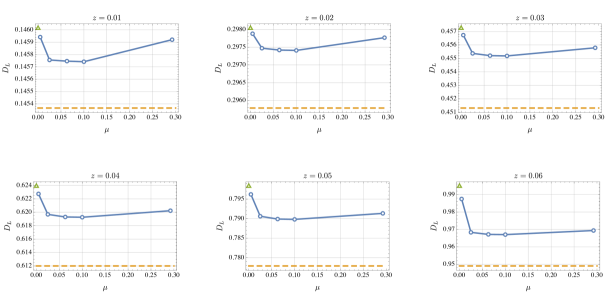
An important remark is that we observe that the tensor modes discussed in Section 4 intensify as $\mu\to 0$, affecting the smaller-$\mu$ BHLs to the point that it becomes impossible to identify a monotonic trend in the luminosity distance for large $z$. For this reason, we are forced to limit our study to very small $z$.

5 Discussion and conclusions

We have investigated the propagation of light along two special curves in the spacetime of a BHL, constructed by numerically integrating Einstein’s equation in 3+1 dimensions. In particular, we have measured the redshift and luminosity distance along these curves, and compared them to the estimates of these observables obtained in suitably fitted homogeneous models and in the EBA. The comparison shows that the latter approximation is the one most capable of reproducing the exact behaviour; we have built a heuristic argument to explain this finding, based on the analysis of the different curvature terms in the GDE. Our finding is congruous with the conclusions of similar studies in other inhomogeneous spacetimes [16]; in our case, however, the models are not backreaction-free by construction, so that we can measure all the relevant contributions to the GDE.

We have also fitted the $D_{\rm L}(z)$ relationship from the FLRW models with both a constant and a $z$-dependent $\Lambda$ to the data, finding that a value of $\Omega_{\Lambda}$ approximately equal to $\Omega_{M}$ reproduces the optical properties of the BHL better than the corresponding models with $\Omega_{\Lambda}=0$. In other words, in the BHL spacetime the luminosity distance for a redshift $z$ is larger than in the corresponding EdS model (the correspondence being based on the same initial proper size and expansion rate). This is also in line with the conclusions of previous studies [18], and arguably equivalent to the finding that fitting $\Omega_{M}$ alternatively leads to a smaller value for this parameter [15].

Finally, we have examined a family of BHLs with varying BH masses and separations, in order to estimate how our result changes as $\mu=M/L\to 0$. In this limit, it was proven in [9] that the expansion history of a BHL tends to that of a flat FLRW model with the same average density. Here, however, we find that the optical properties of a BHL exhibit a finite deviation from the corresponding FLRW model, which reaches $5\%$ by $z=0.06$. Given a considerable pollution by tensor modes, which we conjecture originate in our initial-data construction, the luminosity distance is oscillatory, and we are unable to evaluate the continuum limit for larger $z$.

Building a picture of the mechanisms involved in these results, as well as generalizing it to inhomogeneous spacetimes with different matter content and density profiles, is a particularly intriguing but hard-to-approach task. We can start to tackle it by comparing our results to a recent study [50], which also measured the effects of light propagation in an inhomogeneous model which, unlike the ones considered in this work, was filled with dust. In that investigation, percent-level deviations were detected from the homogeneous Hubble law, which are about an order of magnitude smaller than the deviations reported here. From the arguments presented in this paper, we infer that the discrepancy is largely due to the different representation of the matter filling the two models. The quantitative formulation of this statement is a problem which we reserve for further study.

Appendix A Geodesic equation 3+1 decomposition

The tangent $p^{a}$ to a geodesic satisfies

$$p^{a}\nabla_{a}p^{b}=0\\$$ (A.1)

or, to simplify the following derivation,

$$p^{a}\nabla_{a}p_{b}=0.\\$$ (A.2)

The covariant derivative is expanded in terms of the partial derivative and the Christoffel symbol of the spacetime metric,

$$p^{a}\partial_{a}p_{b}=p^{a}p^{c}\Gamma_{cab}\\$$ (A.3)

and the LHS is recognised as the derivative along the curve of the component $p_{b}$ with respect to the curve parameter,

$$\frac{dp_{b}}{d\lambda}=p^{a}\partial_{a}p_{b}$$ (A.4)

The Christoffel symbol is expressed in terms of derivatives of the metric,

$$p^{a}p^{c}\Gamma_{cab}=\frac{1}{2}p^{a}p^{c}(g_{cb,a}+g_{ac,b}-g_{ab,c})$$ (A.5)

and we note that the first and third terms in parentheses are antisymmetric in $a$ and $c$, whereas $p^{a}p^{c}$ is symmetric, so these terms sum to zero, giving

$$\frac{dp_{b}}{d\lambda}=\frac{1}{2}p^{a}p^{c}g_{ac,b},$$ (A.6)

as the geodesic equation for the covariant component of the tangent vector.

We now wish to express the RHS in terms of the 3+1 quantities available in a numerical relativity simulation. We summarise briefly the standard 3+1 decomposition of a spacetime (see, e.g. [51]). A foliation of constant-time hypersurfaces is represented by a one-form $\Omega_{a}$, which locally can be written as the differential of the coordinate time, $\Omega_{a}=\nabla_{a}t$. The lapse function is defined as $\alpha\equiv(-\Omega_{a}\Omega^{a})^{-1/2}$, and the timelike unit hypersurface normal as $n_{a}\equiv-\alpha\Omega_{a}$, so that $n_{a}n^{a}=-1$. The spatial metric on the hypersurface is

$$\gamma_{ab}=g_{ab}+n_{a}n_{b}$$ (A.7)

with $\gamma_{ab}n^{a}=0$. A vector $S^{a}$ is described as spatial if $S^{a}n_{a}=0$. Since the direction of time evolution, $t^{a}=(\partial/\partial t)^{a}$, is not necessarily aligned with the normal to the hypersurface, we express it in terms of a normal component, and the spatial shift vector $\beta^{a}$,

$$t^{a}=\alpha n^{a}+\beta^{a}.$$ (A.8)

To simplify the expressions, we will work in the standard coordinate basis in which the timelike basis vector is $t^{a}\equiv(\partial/\partial t)^{a}$, and hence has components $[1,0,0,0]$. In such a basis, we have $n_{0}=-\alpha$, $n_{i}=0$, $n^{0}=\alpha^{-1}$, $S^{0}=0$, where $S^{a}$ is any spatial vector, and lower case Latin indices from the middle of the alphabet ($i,j,\ldots$) indicate spatial components (i.e. $i=1,2,3$). These relations will simplify the derivation.

We now need to express equation (A.6) in terms of partial derivatives of the spatial quantities available in an NR simulation. We first decompose $p_{a}$ into a timelike and spatial part,

$$p_{a}=\sigma n_{a}+q_{a}$$ (A.9)

where $q_{a}n^{a}=0$, and aim to find an equation for the evolution of $q_{i}$. Note that $p_{i}=q_{i}$ since $n_{i}$ = 0. Substituting equations (A.7) and (A.9) into equation (A.6), we eventually obtain

$$\frac{dq_{i}}{d\lambda}=\sigma^{2}n^{a}n_{a,i}-\sigma n^{a}_{,i}q^{c}\gamma_{ac}+\frac{1}{2}q^{a}q^{c}\gamma_{ac,i}.$$ (A.10)

In deriving this, we have made use of the fact that all contractions of $(n_{a}n_{c}),_{i}$ with $q^{a}$ vanish, $n_{i}=0$, $n^{a}n^{c}\gamma_{ac,i}=-n^{a}_{,i}n^{c}\gamma_{ac}=0$, since $n^{c}\gamma_{ac}=0$, and that $n^{a}\gamma_{ac,i}=-n^{a}_{,i}\gamma_{ac}$.

We now express $n$ in terms of $\alpha$ and $\beta$ using equation (A.8) to obtain

$$\frac{dq_{i}}{d\lambda}=-\sigma^{a}\alpha^{-1}\alpha_{,i}+\sigma\alpha^{-1}\beta^{a}_{,i}q_{a}-\frac{1}{2}q_{a}q_{c}\gamma^{ac}_{,i}$$ (A.11)

where we have used the fact that $t^{\mu}=\delta^{\mu}_{0}$, hence $t^{\mu}_{,\nu}=0$.

The tangent vector components are related to the coordinates of the curve via $dx^{\mu}/d\lambda=p^{\mu}$. The time component gives $dt/d\lambda=p^{0}=\sigma\alpha^{-1}$ and the spatial components give $dx^{i}/d\lambda=p^{i}$. Using the chain rule, we obtain $d/dt=(p^{0})^{-1}d/d\lambda$, and eliminating $\sigma$ in favour of $p^{0}$, we obtain finally equations (4.11)–(4.13):

$$\frac{dx^{i}}{dt} = -\beta^{i}+(p^{0})^{-1}\gamma^{ik}q_{k}$$ (A.12)

$$\frac{dq_{i}}{dt} = -p^{0}\alpha\alpha_{,i}+q_{j}\beta^{k}_{,i}\gamma_{kj}-\frac{1}{2}(p^{0})^{-1}q_{l}q_{m}\gamma^{lm}_{,i}$$ (A.13)

$$\frac{d\lambda}{dt} = (p^{0})^{-1}$$ (A.14)

in agreement with [48].

Appendix B Geodesic integrator tests

We now present three different tests of the 3+1 Geodesic code against existing known solutions: (i) the redshift-luminosity relationship in an EdS universe, (ii) the geodesics in the Schwarzschild spacetime, and (iii) the geodesics in a model from the Szekeres class.

B.1 Redshift and luminosity distance in the EdS spacetime

In the first test, we check both the redshift and the luminosity distance by letting geodesics propagate in an EdS universe.

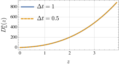
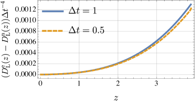
Using our infrastructure, we can propagate null rays on an EdS universe and compare the answer to the analytical solution (2.42). Specifically, we use the code presented in [52] to evolve a periodic cubic domain of this spacetime, with boundaries $-L/2\leq x,y,z\leq L/2$, with $L=20$, starting with the same initial scale factor $a_{\cal S}$ and expansion rate $H_{\cal S}$ as the $M=1$ BHL discussed in section 4. We perform three separate runs with $5^{3}$, $10^{3}$ and $20^{3}$ points, tracking a geodesic that moves from the origin along the $x$ axis (notice that as this type of space is completely homogeneous and isotropic, the curve does not depend on the location of the null rays, but merely on the value of the scale factor at its end points).

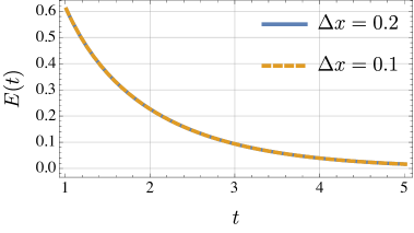
Figure 8 illustrates our result: as expected, the numerical solution converges to the exact equation (2.42) at fourth order.

Figure 8: Luminosity distance as a function of redshift for the Einstein-de Sitter model. Left: the numerical solution $D^{\rm n}_{L}(z)$ for two different resolutions. Right: the difference between the numerical and the exact solution $D^{\rm e}_{L}(z)$ (given by (2.42)) multiplied by $\Delta t^{-4}$ to show fourth-order convergence.

B.2 Geodesics in the Schwarzschild spacetime

We then compare the computation of a geodesic in a numerical Schwarzschild spacetime using the generic 3+1 Geodesic code against a direct numerical integration of the well-known Schwarzschild geodesic equations.

In Schwarzschild, the geodesic equation in the $\theta=\pi/2$ plane reduces to

$$\frac{dt}{d\lambda} = \frac{E}{1-2M/r}$$ (B.1)

$$\frac{d\phi}{d\lambda} = \frac{L}{r^{2}}$$ (B.2)

$$\frac{d^{2}r}{d\lambda^{2}} = -\frac{M}{r^{3}}\left(r-2M\right)\left(\frac{E}{1-2M/r}\right)^{2}+\frac{M}{r(r-2M)}\left(\frac{dr}{d\lambda}\right)^{2}$$ (B.3)

$$+(r-2M)\left(\frac{L}{r^{2}}\right)^{2}$$

where $E$ and $L$ are the conserved energy and angular momentum (see, for example, [53]). Since there is no closed-form solution, we integrate (B.1)–(B.3) numerically using Mathematica.

We then use the 3+1 Geodesic code to integrate the geodesic using the same initial conditions on a uniform Cartesian grid of spacing $\Delta x$ with timestep $\Delta t=2\Delta x$. The metric is expressed in isotropic coordinates, where the relation between isotropic ($R$) and Schwarzschild ($r$) radial coordinates is

$$r=R(1+M/(2R))^{2}.$$ (B.4)

The test null geodesic has initial conditions

$$[R,\theta,\phi] = [8M,0,0]$$ (B.5)

$${[q_{R},q_{\theta},q_{\phi}]} = [\sqrt{2},0,3\pi/4]$$ (B.6)

$$\frac{d\lambda}{dt} = 1.$$ (B.7)

We compute the 3+1 solution using two different grid spacings, $\Delta x=M/4$ and $M/8$, to assess convergence of the solution.

Figure 9: Test of the 3+1 Geodesic code against direct numerical integration of the Schwarzschild geodesic equations. Top: null geodesic trajectory in the $xy$ plane. Bottom: convergence of the affine parameter $\lambda$ and polar coordinates $r,\phi$ to the Schwarzschild geodesic solution. The errors have been rescaled by ${\Delta x}^{-4}$ and the agreement shows fourth order convergence.

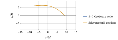
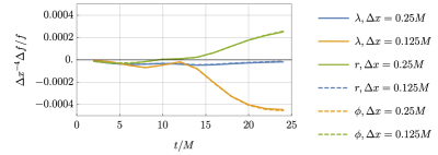
In Figure 9 we plot the trajectories of the Schwarzschild and 3+1 geodesics in the $xy$ plane and see that they agree very well. The numerical integration of the Schwarzschild geodesic equations is much more accurate than the 3+1 solution, so we take the difference between the 3+1 and Schwarzschild solutions to be the error in the 3+1 solution. In Figure 9, we also plot the error for the three components of the solution, $\lambda(t)$, $r(t)$ and $\phi(t)$ multiplied by ${\Delta x}^{-4}$ for the two different values of $\Delta x$. The curves agree well, indicating that the 3+1 Geodesic code produces a result which converges at fourth order to the Schwarzschild geodesic solution,

$$f_{\mathrm{3+1}}-f_{\mathrm{Sch}}=O({\Delta x}^{4}).$$ (B.8)

The observed fourth order convergence is consistent with the expected dominant error from the fourth-order Runge-Kutta time integrator.

B.3 Geodesics in a spacetime from the Szekeres class

A less trivial testbed is provided by the Szekeres class of inhomogeneous cosmological models. We use, in particular, the axisymmetric solution described by Meures and Bruni [54, 55], given by the line element:

$$ds^{2}=-dt^{2}+S(t)^{2}\left[dx^{2}+dy^{2}+Z(t,z)^{2}dz^{2}\right]$$ (B.9)

with

$$S(t)=\left(\frac{1-\Omega_{\Lambda}}{\Omega_{\Lambda}}\right)^{1/3}\sinh^{2/3}\left[\frac{3}{2}H_{0}\sqrt{\Omega_{\Lambda}}(t+t_{\star})\right]$$ (B.10)

$$Z(t,z)=1+(1-\sin kz)[f_{+}(t+t_{\star})+B(x^{2}+y^{2})]$$ (B.11)

and $\Lambda$, $\Omega_{\Lambda}$, $k$ and $B$ are the cosmological constant and its associated density parameter, an arbitrary wave number, and a constant given by:

$$B=\frac{3}{4}H_{0}^{2}\left[\Omega_{\Lambda}(1-\Omega_{\Lambda})^{2}\right]^{1/3},$$ (B.12)

respectively. Finally, $f_{+}(t)$ is a solution of:

$$f^{\prime\prime}+\frac{4}{3}\coth\left(\sqrt{\frac{3\Lambda}{4}}t\right)f^{\prime}-\frac{2}{3}\frac{1}{\sinh^{2}\left(\sqrt{\frac{3\Lambda}{4}}t\right)}f=0.$$ (B.13)

In [55], an ODE system for the geodesics propagating on this spacetime is provided. For geodesics propagating along the symmetry axis $x=y=0$, this system has the simplified form [55]:

$$-\frac{E^{\prime}}{E}-\frac{S^{\prime}}{S}-\frac{\dot{F}}{1+F}=0$$ (B.15)

$$z^{\prime}-\frac{2}{3}\frac{1}{H_{0}\sqrt{\Omega_{\Lambda}}SZ}=0$$

where $E$ is the photon energy along the geodesic and $z$ is its coordinate. Primes indicate derivatives with respect to the rescaled time $\tau=\sqrt{3\Lambda/4}t$. As in the Schwarzschild test, we solve this system with Mathematica.

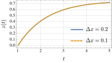
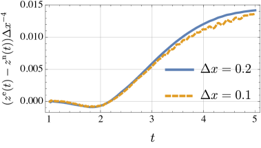
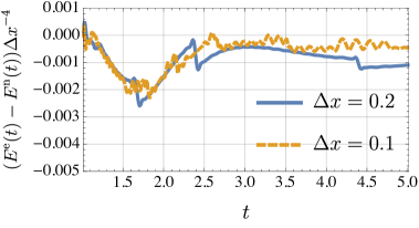
As in [52], we compute the metric of this spacetime on a cubic domain $[-L/2,L/2]^{3}$, with $L=2$, and at two different resolutions $\Delta x={0.1,0.2}$. Figure 10 shows the comparison between the numerical computations and the solution of (B.15)-(B.15). The agreement is compatible with fourth-order convergence, as expected.

Figure 10: Geodesic location and associated photon redshift for a geodesic starting at the origin and parallel to the $z$ axis in the Szekeres model.

References

- [1] C.-M. Yoo, H. Abe, K.-i. Nakao, and Y. Takamori, Black Hole Universe: Construction and Analysis of Initial Data, Phys.Rev. D86 (2012) 044027, [arXiv:1204.2411].
- [2] E. Bentivegna and M. Korzyński, Evolution of a periodic eight-black-hole lattice in numerical relativity, Class.Quant.Grav. 29 (2012) 165007, [arXiv:1204.3568].
- [3] C.-M. Yoo, H. Okawa, and K.-i. Nakao, Black Hole Universe: Time Evolution, Phys.Rev.Lett. 111 (2013) 161102, [arXiv:1306.1389].
- [4] E. Bentivegna and M. Korzyński, Evolution of a family of expanding cubic black-hole lattices in numerical relativity, Class.Quant.Grav. 30 (2013) 235008, [arXiv:1306.4055].
- [5] C.-M. Yoo and H. Okawa, Black Hole Universe with , Phys.Rev. D89 (2014) 123502, [arXiv:1404.1435].
- [6] T. Clifton, D. Gregoris, K. Rosquist, and R. Tavakol, Exact Evolution of Discrete Relativistic Cosmological Models, JCAP 1311 (2013) 010, [arXiv:1309.2876].
- [7] T. Clifton, D. Gregoris, and K. Rosquist, Piecewise Silence in Discrete Cosmological Models, Class.Quant.Grav. 31 (2014) 105012, [arXiv:1402.3201].
- [8] M. Korzyński, I. Hinder, and E. Bentivegna, On the vacuum Einstein equations along curves with a discrete local rotation and reflection symmetry, JCAP 1508 (2015), no. 08 025, [arXiv:1505.05760].
- [9] M. Korzyński, Backreaction and continuum limit in a closed universe filled with black holes, Class.Quant.Grav. 31 (2014) 085002, [arXiv:1312.0494].
- [10] P. Fleury, Cosmic backreaction and Gauss’s law, arXiv:1609.03724.
- [11] Y. B. Zeldovich, Observations in a Universe Homogeneous in the Mean, Soviet Astronomy 8 (Aug., 1964) 13.
- [12] C. C. Dyer and R. C. Roeder, The Distance-Redshift Relation for Universes with no Intergalactic Medium, Astrophys. J. 174 (June, 1972) L115.
- [13] C. Dyer and R. Roeder, Distance-Redshift Relations for Universes with Some Intergalactic Medium, Astrophys.J. 180 (1973) L31.
- [14] P. Fleury, H. Dupuy, and J.-P. Uzan, Interpretation of the Hubble diagram in a nonhomogeneous universe, Phys. Rev. D87 (2013), no. 12 123526, [arXiv:1302.5308].
- [15] P. Fleury, H. Dupuy, and J.-P. Uzan, Can all cosmological observations be accurately interpreted with a unique geometry?, Phys. Rev. Lett. 111 (2013) 091302, [arXiv:1304.7791].
- [16] P. Fleury, Swiss-cheese models and the Dyer-Roeder approximation, JCAP 1406 (2014) 054, [arXiv:1402.3123].
- [17] T. Clifton and P. G. Ferreira, Archipelagian Cosmology: Dynamics and Observables in a Universe with Discretized Matter Content, Phys. Rev. D80 (2009) 103503, [arXiv:0907.4109]. [Erratum: Phys. Rev.D84,109902(2011)].
- [18] T. Clifton and P. G. Ferreira, Errors in Estimating due to the Fluid Approximation, JCAP 0910 (2009) 026, [arXiv:0908.4488].
- [19] T. Clifton, P. G. Ferreira, and K. O’Donnell, An Improved Treatment of Optics in the Lindquist-Wheeler Models, Phys. Rev. D85 (2012) 023502, [arXiv:1110.3191].
- [20] J.-P. Bruneton and J. Larena, Observables in a lattice Universe, Class. Quant. Grav. 30 (2013) 025002, [arXiv:1208.1411].
- [21] S. Seitz, P. Schneider, and J. Ehlers, Light propagation in arbitrary space-times and the gravitational lens approximation, Class.Quant.Grav. 11 (1994) 2345–2374, [astro-ph/9403056].
- [22] R. Sachs, Gravitational waves in general relativity. vi. the outgoing radiation condition, Proceedings of the Royal Society of London A: Mathematical, Physical and Engineering Sciences 264 (1961), no. 1318 309–338.
- [23] V. Perlick, Gravitational lensing from a spacetime perspective, Living Reviews in Relativity 7 (2004), no. 9 [arXiv:1010.3416].
- [24] I. Etherington, Republication of: Lx. on the definition of distance in general relativity, General Relativity and Gravitation 39 (2007) 1055–1067.
- [25] D. W. Hogg, Distance measures in cosmology, astro-ph/9905116.
- [26] J. Kristian and R. K. Sachs, Observations in Cosmology, Astrophysical Journal 143 (Feb., 1966) 379.
- [27] J. E. Gunn, On the Propagation of Light in Inhomogeneous Cosmologies. I. Mean Effects, Astrophys. J. 150 (Dec., 1967) 737.
- [28] R. Kantowski, Corrections in the Luminosity-Redshift Relations of the Homogeneous Fried-Mann Models, Astrophys. J. 155 (Jan., 1969) 89.
- [29] S. Refsdal, On the Propagation of Light in Universes with Inhomogeneous Mass Distribution, Astrophys. J. 159 (Jan., 1970) 357.
- [30] V. Lamburt, D. Sokoloff, and V. Tutubalin, Light propagation in a universe with spatial inhomogeneities, Astrophysics and Space Science 298 (2005), no. 3 409–418.
- [31] K. Bolejko and M.-N. Célérier, Szekeres Swiss-cheese model and supernova observations, Phys. Rev. D 82 (Nov., 2010) 103510, [arXiv:1005.2584].
- [32] S. J. Szybka, Light propagation in Swiss-cheese cosmologies, Phys. Rev. D 84 (Aug., 2011) 044011, [arXiv:1012.5239].
- [33] A. Nwankwo, M. Ishak, and J. Thompson, Luminosity distance and redshift in the Szekeres inhomogeneous cosmological models, JCAP 1105 (2011) 028, [arXiv:1005.2989].
- [34] C. Clarkson, G. F. R. Ellis, A. Faltenbacher, R. Maartens, O. Umeh, and J.-P. Uzan, (Mis)interpreting supernovae observations in a lumpy universe, Month. Not. Roy. Astr. Soc. 426 (Oct., 2012) 1121–1136, [arXiv:1109.2484].
- [35] K. Bolejko and P. G. Ferreira, Ricci focusing, shearing, and the expansion rate in an almost homogeneous Universe, JCAP 5 (May, 2012) 3, [arXiv:1204.0909].
- [36] M. Lavinto, S. Räsänen, and S. J. Szybka, Average expansion rate and light propagation in a cosmological Tardis spacetime, JCAP 1312 (2013) 051, [arXiv:1308.6731].
- [37] M. Troxel, M. Ishak, and A. Peel, The effects of structure anisotropy on lensing observables in an exact general relativistic setting for precision cosmology, JCAP 1403 (2014) 040, [arXiv:1311.5936].
- [38] S. Bagheri and D. J. Schwarz, Light propagation in the averaged universe, JCAP 1410 (2014), no. 10 073, [arXiv:1404.2185].
- [39] A. Peel, M. A. Troxel, and M. Ishak, Effect of inhomogeneities on high precision measurements of cosmological distances, Phys. Rev. D90 (2014), no. 12 123536, [arXiv:1408.4390]. [Erratum: Phys. Rev.D92,no.2,029901(2015)].
- [40] V. Marra, M. Paakkonen, and W. Valkenburg, Uncertainty on w from large-scale structure, Mon. Not. Roy. Astron. Soc. 431 (2013) 1891–1902, [arXiv:1203.2180].
- [41] F. Steiner, Do Black Holes Exist in a Finite Universe Having the Topology of a Flat 3-Torus?, arXiv:1608.03133.
- [42] Cactus code: http://www.cactuscode.org.
- [43] E. Schnetter, S. H. Hawley, and I. Hawke, Evolutions in 3-D numerical relativity using fixed mesh refinement, Class. Quant. Grav. 21 (2004) 1465–1488, [gr-qc/0310042].
- [44] Carpet code: https://www.carpetcode.org.
- [45] McLachlan code: https://www.cct.lsu.edu/~eschnett/McLachlan.
- [46] Kranc code: http://kranccode.org.
- [47] E. Bentivegna, Solving the Einstein constraints in periodic spaces with a multigrid approach, Class.Quant.Grav. 31 (2014) 035004, [arXiv:1305.5576].
- [48] S. A. Hughes, C. R. Keeton, P. Walker, K. T. Walsh, S. L. Shapiro, and S. A. Teukolsky, Finding black holes in numerical space-times, Phys. Rev. D49 (1994) 4004–4015.
- [49] E. A. Milne, A newtonian expanding universe, The Quarterly Journal of Mathematics os-5 (1934), no. 1 64–72.
- [50] J. T. Giblin, J. B. Mertens, and G. D. Starkman, Observable Deviations from Homogeneity in an Inhomogeneous Universe, Astrophys. J. 833 (2016), no. 2 247, [arXiv:1608.04403].
- [51] M. Alcubierre, Introduction to 3+1 Numerical Relativity. International Series of Monographs on Physics. OUP Oxford, 2008.
- [52] E. Bentivegna, An automatically generated code for relativistic inhomogeneous cosmologies, arXiv:1610.05198.
- [53] S. M. Carroll, Spacetime and geometry: An introduction to general relativity. 2004.
- [54] N. Meures and M. Bruni, Redshift and distances in a CDM cosmology with non-linear inhomogeneities, Mon.Not.Roy.Astron.Soc. 419 (2012) 1937, [arXiv:1107.4433].
- [55] N. Meures and M. Bruni, Exact non-linear inhomogeneities in CDM cosmology, Phys. Rev. D83 (2011) 123519, [arXiv:1103.0501].