Performance enhancement of non-minimum phase feedback systems by fractional-order cancellation of non-minimum phase zero on the Riemann surface: New theoretical and experimental results

Abstract

The non-minimum phase (NMP) zero of a linear process located in the feedback connection cannot be cancelled by the same pole of controller according to the internal instability problem. However, such a zero can partly be cancelled by the same fractional-order pole of a pre-compensator located in series with process without facing internal instability. This paper first presents new theoretical results on the properties of this method of cancellation, and provides design techniques for the pre-compensator. It is especially shown that by appropriate design of pre-compensator this method can simultaneously increase the gain and phase margin of the system under control without a considerable reduction of open-loop bandwidth, and consequently, it can make the control problem easier to solve. Then, a method for realization of such a pre-compensator is proposed and performance of the resulted closed-loop system is studied through an experimental setup. non-minimum phase zero, performance limitation, partial zero-pole cancellation, experimental result, Riemann surface.

1 Introduction

In the field of linear time-invariant systems, a process is identified as a non-minimum phase (NMP) system if its transfer function has at least one right half-plane (RHP) zero, or a RHP pole, or a time delay. Among others, systems with RHP zero(s) constitute a very important category of NMP systems, both from theoretical and practical point of view. Such zeros appear in many real-world systems such as flexible link robots [1, 2], step-up DC-DC converters [3, 4], floating-wind turbines [5], aircrafts [6], bicycles [7], driving a car backwards [8], continuous stirred tank reactors [9], nano positioning devices [10], and many others.

One classical fact in relation to NMP zeros is that they cannot be cancelled by the same poles of controller according to the internal instability problem [11]. The other well-known fact is that NMP zeros of the process put some limitations on the performance of the corresponding feedback system [12]. One main reason for this limitation is that in order to achieve a good command following and disturbance rejection behavior, any feedback system needs large open-loop gains at lower frequencies, which is often provided by the controller [11]. On the other hand, according to the classical root-locus method, any closed-loop system has the property that its poles move towards open-loop zeros as the gain in the loop is increased. Hence, there is a tradeoff between performance and stability when the process has a NMP zero since the open-loop gain cannot be increased arbitrarily in this case. It should be noted that many other controller design techniques also strictly depend on the possibility of applying large gains in the loop. For example, successful application of the loop transfer recovery (LTR) method needs using large gains in the loop [11]. That is why application of LTR is mainly limited to minimum phase processes.

The difficulty of controlling NMP processes can also be explained through frequency domain analysis. More precisely, a process with a NMP zero is more phase-lag compared to the one which has a zero with the same amplitude but at the left half-plane. This extra phase-lag puts a limitation on the gain of controller since increasing the loop gain increases the gain crossover frequency which often leads to decreasing the PM. Again, considering the fact that large open-loop gains at low frequencies are essential for command following and disturbance rejection, it is obvious that NMP zero puts a serious restriction on the performance of the closed-loop system.

Very recently the idea of partial cancellation of the NMP zero of process on the Riemann surface is proposed in [13]. It is especially shown in that paper that partial cancellation of the NMP zero of process leads to a transfer function with fractional-order zero which can be controlled more easily compared to the original NMP process. However, no routine design technique is presented in that paper. This paper completes the basic idea proposed in [13] both from theoretical and experimental aspects. The main idea behind the methods proposed in this paper for partial cancellation of NMP zero is that in dealing with many real-world processes, smaller the value of $\kappa\triangleq|P(j\omega_{u})/P(0)|$ more easier its control [14], where $P(s)$ is the transfer function of process and $\omega_{u}$ is the ultimate frequency, i.e. $\angle P(j\omega_{u})=-180^{\circ}$ (as a rule of thumb, processes with $\kappa<0.4$ are considered as easier control problems [14]). Hence, the aim of this paper is to design a pre-compensator for partial cancellation of NMP zero such that the resulted system has a larger gain and phase margin, and consequently, be easier to control.

The rest of this paper is organized as the following. Some preliminaries, which will be instrumental in the discussions of next sections, are presented in Section 2. The method of partial cancellation of NMP zero of process on the Riemann surface is also briefly reviewed in this section. Some new theoretical results on this subject are presented in Section 3. Specially, two methods for designing the partial canceller of NMP zero are proposed in this section. A novel NMP benchmark circuit is presented in Section 4 and the proposed design techniques for canceller are successfully tested on this benchmark. Finally, Section 5 concludes the paper.

2 Preliminaries and review of previous findings

Some basic definitions, which will be instrumental in the discussions of the next sections, are presented in this section. Some of the material presented in this section can also be found with more details in [13]. Consider the unity feedback system shown in Fig. 1 where $P(s)$ is the NMP transfer function of process, $C_{canc}(s)$ is the pre-compensator used to partially cancel the NMP zero of $P(s)$ on Riemann surface, and $C(s)$ is the controller designed to control the augmented process $C_{canc}(s)P(s)$. (In the rest of this paper the terms “canceller” and “pre-compensator” are used to refer to $C_{canc}(s)$ interchangeably. Moreover, in this paper the series connection of $C_{canc}(s)$ and $P(s)$ is called the “augmented process” since the controller $C(s)$ has to be designed for a process with transfer function $C_{canc}(s)P(s)$ which is easier to control compared to $P(s)$ provided that $C_{canc}(s)$ is suitably designed.) For a better and more clear understanding the effect of proposed canceller on the function of closed-loop system, the discussions of this paper are presented assuming proportional controller in the loop, i.e., without a considerable loss of generality it is assumed that the controller $C(s)$ in Fig. 1 is in the form of a simple constant gain. However, the main results can easily be extended to more complicated controllers.

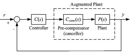
Figure 1: Feedback system with pre-compensator for partial cancellation of the NMP zero of process. $P(s)$ and $C_{canc}(s)$ are defined in (2.1) and (2.2), respectively.

In the rest of this paper it is assumed that the transfer function of NMP process in Fig. 1 can be decomposed as the following

$$P(s)=\left(1-\frac{s}{z_{nmp}}\right)\widetilde{P}(s),$$ (2.1)

where $(1-s/z_{nmp})$ is the NMP zero term of $P(s)$ and $z_{nmp}>0$ is the NMP zero. As a very well-known classical fact [11], neither $C(s)$ nor $C_{canc}(s)$ can have a pole at $s=z_{nmp}$ according to the internal instability problem, i.e., any zero-pole cancellation in the RHP is impractical since the resulted system is internally unstable. Considering the fact that in the feedback connection of Fig. 1 the closed-loop zeros are the same as open-loop zeros, it is concluded that one has to tolerate the limitations caused by NMP zeros since they appear unavoidably in the closed-loop transfer function. However, it is shown in [13] that it is possible to partly cancel the NMP zero of $P(s)$ by $C_{canc}(s)$ on the Riemann surface and arrive at a higher performance feedback system. More precisely, similar to [13], here the transfer function of canceller is considered as

$$C_{canc}(s)=\frac{1}{\sum_{k=1}^{n}\left(\frac{s}{z_{nmp}}\right)^{(k-1)/n}},$$ (2.2)

where $n$ is the design parameter which determines the order of cancellation of NMP zero [13]. (To follow the discussions in this paper one does not need to have a deep knowledge about fractional calculus and the time-domain interpretation of fractional powers of $s$ in (2.2). See [15] for more details on this subject). It is shown in [13] that the series connection of $P(s)$ and $C_{canc}(s)$, as defined in (2.1) and (2.2), respectively, is as the following

$$C_{canc}(s)P(s)=\left[1-\left(\frac{s}{z_{nmp}}\right)^{1/n}\right]\widetilde{P}(s),$$ (2.3)

which, unlike $P(s)$, has a fractional-order NMP zero at $s=z_{nmp}$ (note that both the $P(s)$ and $C_{canc}(s)P(s)$ have exactly the same poles and zeros, and the only difference between these two transfer functions is that $C_{canc}(s)P(s)$ has a fractional-order NMP zero at $s=z_{nmp}$). Assuming

$$F(s)=1-\left(\frac{s}{z_{nmp}}\right)^{\alpha},$$ (2.4)

one can further write (2.3) as $C_{canc}(s)P(s)=F(s)\widetilde{P}(s)$ for $\alpha=1/n$. In brief, the effect of canceller is that it changes the NMP term $1-s/z_{nmp}$ at the numerator of $P(s)$ to $1-(s/z_{nmp})^{\alpha}$ for some rational $\alpha$ smaller than unity.

As another definition, in the rest of this paper $L_{canc}(s)$ and $L(s)$ denote the open-loop transfer functions with and without applying the canceller, respectively. That is

$$L(s)=C(s)P(s),$$ (2.5)

and

$$L_{canc}(s)=C(s)C_{canc}(s)P(s).$$ (2.6)

The gain crossover frequency of the open-loop transfer function with canceller is denoted as $\omega_{gc}$, that is $|L_{canc}(j\omega_{gc})|=0$ dB.

3 Theoretical Findings and the Proposed Design Methods for Pre-compensator

3.1 Effect of canceller on the open-loop frequency response

One intrinsic characteristic of any zero (either NMP or MP) is that it leads to increment in the amplitude of the frequency response of the corresponding transfer function as the frequency is increased. For example, in the numerator of (2.1) amplitude of the term $\left(1-s/z_{nmp}\right)_{s=j\omega}$ is monotonically increased by increasing $\omega$. This increase in the amplitude of open-loop transfer function increases the gain crossover frequency of system and simultaneously makes it more phase lag if the zero is NMP. Hence, it is expected that a feedback system with a NMP zero in the loop exhibits a very poor stability if the bandwidth is sufficiently large. But, surprisingly, the partly-cancelled NMP term $\left[1-(s/z_{nmp})^{\alpha}\right]_{s=j\omega}$ ($0<\alpha<1$) has the property that its amplitude is monotonically decreased by increasing $\omega$ in the frequency range $[0,\omega_{min}]$ where $\omega_{min}=\left[\cos(\pi\alpha/2)\right]^{1/\alpha}z_{nmp}$ [13] (see Fig. 2 for more details). It concludes that, as it can be observed in Fig. 2, this partly-cancelled NMP term in the numerator of open-loop transfer function somehow acts as a stable pole in this frequency range. Considering the fact that in practice the gain crossover frequency of any NMP system is often approximately limited to the frequency of its NMP zero [16, 17], this pole-like behavior of the partly-cancelled NMP zero can improve the gain-bandwidth of system since it considerably decreases the amplitude of open-loop frequency response at frequencies around $\omega=z_{nmp}$, while it has a negligible effect at lower frequencies. In the following, we study the frequency response of the partly cancelled zero term (2.4) mathematically assuming $\omega_{gc}=z_{nmp}$; however, the main results can be extended to values of $\omega_{gc}\neq z_{nmp}$ as well.

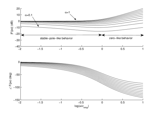
Figure 2: Bode plots of the partly-cancelled zero term $F(s)=\left[1-(s/z_{nmp})^{\alpha}\right]_{s=j\omega}$ ($z_{nmp}>0$) versus the normalized frequency for $\alpha=0.1,0.2,\ldots,1$. In a certain frequency range the magnitude and phase plots are decreased simultaneously as the frequency is increased, which is similar to the behavior of a stable pole.

For the partly cancelled NMP term given in (2.4) trivial calculations yield

$$|F(j\omega)|_{\omega=z_{nmp}}=\left|1-\left(j\frac{\omega}{z_{nmp}}\right)^{\alpha}\right|_{\omega=z_{nmp}}=\sqrt{2-2\cos\frac{\pi\alpha}{2}}.$$ (3.1)

It is concluded from (3.1) that $|F(jz_{nmp})|<1$ for $\alpha<2/3$. It means that in the feedback system shown in Fig. 1 application of canceller changes the NMP term of process from $1-s/z_{nmp}$ to $1-(1/z_{nmp})^{\alpha}$ which, assuming $0<\alpha<2/3$, reduces the open-loop gain at the frequency of NMP zero (which is often close to the gain crossover frequency of system in practice) as the following

$$|L_{canc}(jz_{nmp})|-|L(jz_{nmp})| =\left|1-\frac{s}{z_{nmp}}\right|_{s=jz_{nmp}}-\left|1-\left(\frac{s}{z_{nmp}}\right)^{\alpha}\right|_{s=jz_{nmp}}$$ (3.2)

$$=\sqrt{2}-\sqrt{2-2\cos\frac{\pi\alpha}{2}}$$ (3.3)

$$=\sqrt{2}\left(1-\sqrt{1-\cos\frac{\pi\alpha}{2}}\right).$$ (3.4)

(Recall that, except the NMP term, $L_{canc}(s)$ is exactly the same as $L(s)$. That is why the difference between the amplitude of open-loop transfer functions in (3.2) is expressed only in terms of the NMP zero terms.) Reduction of open-loop gain as given in (3.4) leads to reduction of gain crossover frequency.

Two points should be noted here. First, although the amplitude of open-loop transfer function at the frequency of NMP zero is reduced after cancellation as given in (3.4), one cannot conclude that assuming $\omega_{gc}=z_{nmp}$ the GM is also increased in the same way. The reason is that the cancellation also makes the system more phase lag as described below (i.e., if $\angle L(j\omega_{0})=-180^{\circ}$ for some $\omega_{0}$ then $\angle L_{canc}(j\omega_{1})=-180^{\circ}$ for some $\omega_{1}<\omega_{0}$). Second, although the above discussion studies the behavior of $|F(j\omega)|$ at $\omega=z_{nmp}$, it is generally true that the proposed cancellation strategy reduces the amplitude of open-loop transfer function at the gain crossover frequency even if $\omega_{gc}\neq z_{nmp}$; however, the amount of this reduction cannot be calculated from (3.4). The proof of this statement is obvious from Fig. 2.

Now we can study the phase behavior of the partly cancelled NMP zero term. For the $F$ defined in (2.4) we have

$$\angle F(j\omega)\big{|}_{\omega=z_{nmp}}=\angle\left[1-\left(j\frac{\omega}{z_{nmp}}\right)^{\alpha}\right]_{\omega=z_{nmp}}=-\frac{\pi}{2}+\frac{\pi\alpha}{4}.$$ (3.5)

Considering the fact that $\angle\left[1-s/z_{nmp}\right]_{s=jz_{nmp}}=-\pi/4$, it is concluded from (3.5) that application of the fractional-order canceller makes the open-loop system $(\alpha-1)\pi/4$ rad more phase-lag at the frequency of NMP zero. More precisely,

$$\angle L_{canc}(jz_{nmp})=\angle L(jz_{nmp})-\frac{(1-\alpha)\pi}{4}.$$ (3.6)

It is concluded from (3.4) and (3.6) that fractional-order cancellation of NMP zero firstly decreases the amplitude of the open-loop transfer function at the gain crossover frequency (as well as other frequencies), which makes the system more stable by increasing its GM, and secondly, makes the open-loop system more phase lag at this frequency, which decreases the PM. Hence, the proposed canceller provides us with a tradeoff between increasing the GM and decreasing the PM. The discussions of the next section provide us with a method to design the canceller such that even both of the GM and PM are increased simultaneously at the cost of slight decrement in the open-loop gain crossover frequency (or equivalently, open-loop and closed-loop bandwidths).

3.2 Designing a suitable pre-compensator for partial cancellation of NMP

Consider again the unity feedback system shown in Fig. 1 where $P(s)$ and $C_{canc}(s)$ are defined as given in (2.1) and (2.2), respectively. In the following, two methods for designing a canceller for partial cancellation of the NMP zero of $P(s)$ on the Riemann surface are proposed. Before presenting these two methods it should be noted that the main reason for using canceller is to arrive at the augmented plant $C_{canc}(s)P(s)$ which has better properties compared to $P(s)$ (e.g., smaller undershoot, higher PM, etc.) and can be controlled more effectively. For this purpose, in the following discussions only the feedback control of augmented plant by means of a proportional controller is studied. Simplicity of proportional controller lets us clearly understand the function of proposed canceller. Of course, after designing the canceller and adjusting the gain of proportional controller to the suitable value one can use any desired method to design a new controller for the resulted augmented plant $K_{p}C_{canc}(s)P(s)$, where $K_{p}$ is equal to the gain of proportional controller. Hence, the results obtained in the following can be extended to more complicated controllers as well.

3.2.1 Designing a canceller to increase the DC gain and keep PM unchanged

The first method proposed here for partial cancellation of NMP zero on the Riemann surface is based on designing a canceller and proportional controller such that the open-loop systems with and without using canceller have the same PM while the former has a larger DC gain. It means that application of canceller makes it possible to use controllers with larger gains in the loop without affecting the stability properties of system. For this purpose consider Fig. 3 which shows the general relation between the Bode plots of $K_{p1}P(s)$, $K_{p1}C_{canc}(s)P(s)$, and $K_{p2}C_{canc}(s)P(s)$ for some $K_{p2}>K_{p1}$ ($K_{p1}$ and $K_{p2}$ denote two different values for the gain of proportional controller in Fig. 1). Note that according to Fig. 2 amplitude of $1-(s/z_{nmp})^{\alpha}$ (which appears in the numerator of $K_{p1}C_{canc}(s)P(s)$) is smaller than the amplitude of $1-s/z_{nmp}$ (which appears at the numerator of $K_{p1}P(s)$) at all frequencies. It concludes that we have $|K_{p1}C_{canc}(j\omega)P(j\omega)|<|K_{p1}P(j\omega)|$ for all $\omega$ as it can be observed in Fig. 3. It also results in the fact that the gain crossover frequency of $K_{p1}C_{canc}(s)P(s)$ is necessarily smaller than $K_{p1}P(s)$. Recall that all terms in the numerator and denominator of $K_{p1}C_{canc}(s)P(s)$ and $K_{p1}P(s)$, except the term cancelled by canceller, are exactly the same.

In order to explain the proposed design method, first assume that in the feedback system shown in Fig. 1 we have $C_{canc}(s)=1$ and the gain of proportional controller is chosen such that the resulted closed-loop system has a certain PM. The solid curve in Fig. 3 shows the Bode plot of $K_{p1}P(s)$ where $K_{p1}$ is the gain of proportional controller to achieve the desired PM, and points $A$ and $B$ denote the gain crossover frequency of the resulted open-loop system and the corresponding phase lag at this frequency, respectively. If in this feedback system we add the canceller block in series with plant (assuming the same value for the gain of proportional controller and a certain value for $\alpha$) we arrive at a feedback system whose Bode plot is shown by the dotted curve in Fig. 3. As mentioned earlier, the canceller has the property that necessarily decreases the gain crossover frequency and makes the system more phase lag at all frequencies as it can be observed in Fig. 3. According to this figure if we want the feedback system with canceller has the same PM as it had before using it, we must increase the gain of proportional controller from $K_{p1}$ to the suitably chosen value $K_{p2}$. More precisely, the value of $K_{p2}$ must be chosen such that the phase lag of $K_{p2}C_{canc}(s)P(s)$ (point $C$) at its gain crossover frequency (point $E$) be equal to the phase lag of $K_{p1}P(s)$ (point $B$) at its gain crossover frequency (point $A$). For this purpose, the required increment in $K_{p1}$ to arrive at $K_{p2}$ is equal to the vertical distance between points $D$ and $E$. In other words, after applying the canceller, the Bode magnitude plot of the open-loop system drops and we need to increase the gain of proportional controller to move it upward such that the phase of open-loop system with canceller at the new gain crossover frequency becomes equal to the one it was before applying the canceller. Note that as it can be observed in Fig. 3 the phase plots of $K_{p2}C_{canc}(s)P(s)$ and $K_{p1}P(s)$ are exactly the same.

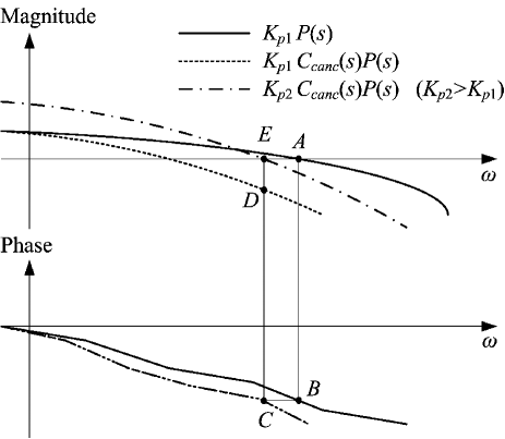
Figure 3: The design procedure for canceller and proportional controller to arrive at a feedback system with increased DC gain (the PM remains the same as before applying the canceller).

To sum up the design procedure, consider a feedback system with the open-loop transfer function $K_{p1}P(s)$ (solid curve in Fig. 3) where the value of $K_{p1}$ is chosen such that the phase lag of $K_{p1}P(s)$ (point $B$) at its gain crossover frequency (point $A$) be equal to the desired value. Apply the canceller in series with $K_{p1}P(s)$ assuming a certain value for $\alpha$ to arrive at a feedback system with the open-loop transfer function shown by dotted curve in Fig. 3. Then increase the gain of proportional controller from $K_{p1}$ to $K_{p2}$ to adjust the gain crossover frequency such that the PM becomes equal to the one it was before applying the canceller (i.e., move point $D$ to $E$ in Fig. 3 by increasing the gain of proportional controller from $K_{p1}$ to $K_{p2}$). The resulted feedback system with canceller has the same PM as it had before applying the canceller while the DC gain and the corresponding tracking and disturbance rejection errors are smaller. Note that using smaller values for $\alpha$ increases the maximum of achievable DC gain at the cost of decreasing the gain crossover frequency. Note also that one can design a controller for the resulted augmented plant $K_{p2}C_{canc}(s)P(s)$ using any desired method by facing less limitations caused by the NMP zero.

In general, it is also possible to design the proportional controller and canceller such that both the PM and open-loop DC gain (or equivalently, gain of proportional controller) are increased simultaneously. The design procedure is very similar to the previous routine and the details are shown in Fig. 4. To sum up, first determine the value of $K_{p1}$ such that $K_{p1}P(s)$ has the desired phase lag (or equivalently, the desired PM) at the gain crossover frequency, as identified by point $B$ in Fig. 4. Next, determine point $C$ on the Bode phase plot of $K_{p1}C_{canc}(s)P(s)$ (assuming a certain value for $\alpha$), which is less phase lag compared to point $B$ to a desired value. More precisely, the vertical difference between points $B$ and $C$ determines the required increment in the PM. Then, increase the gain of proportional controller from $K_{p1}$ to $K_{p2}$ such that point $D$ on the Bode magnitude plot of $K_{p1}C_{canc}P(s)$ moves to point $E$ on the Bode magnitude plot of $K_{p2}C_{canc}P(s)$. In this manner the phase lag of $K_{p2}C_{canc}P(s)$ at its gain cross over frequency (identified as point $E$) becomes equal to point $C$ (note that point $C$ is less phase lag than the original system $K_{p1}P(s)$ at its gain crossover frequency). Clearly, one can also design a controller for the resulted augmented plant $K_{p2}C_{canc}P(s)$ to arrive at a higher performance feedback system.

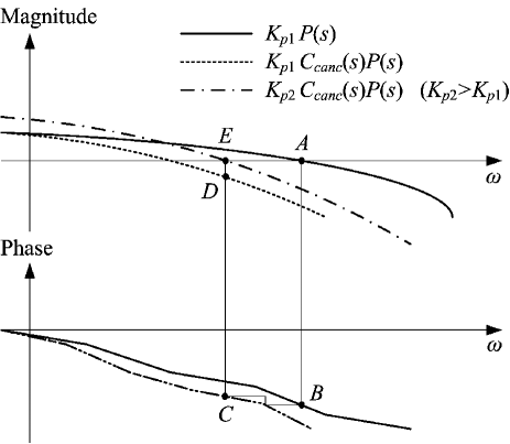
Figure 4: The design procedure for canceller and proportional controller to arrive at a feedback system with increased PM and DC gain.

3.2.2 Designing a canceller to increase PM and keep the DC gain unchanged

The second possible approach is to design the canceller such that the feedback systems with and without using canceller have the same DC gain while the system with canceller has a larger PM. For this purpose consider again the feedback system shown in Fig. 1 where assuming $C_{canc}(s)=1$ and $C(s)=K_{p1}$ the corresponding open-loop transfer function $K_{p1}P(s)$ has a certain phase lag (point $B$ in Fig. 5) at its gain crossover frequency (point $A$ in Fig. 5). According to the previous discussions, application of canceller decreases the gain crossover frequency and simultaneously makes the open-loop system more phase lag as shown by the dash-dotted curve in Fig. 5. Now, consider the canceller in series with plant (assuming the same value for the gain of proportional controller) and determine the value of $\alpha$ by trial and error such that the phase of $K_{p1}C_{canc}(s)P(s)$ (point $C$ in Fig. 5) at its gain crossover frequency (point $D$) be larger than the phase of $K_{p1}P(s)$ (point $B$) at its gain crossover frequency (point $A$). Clearly, the increment in PM is equal to the vertical difference between points $B$ and $C$, which is obtained at the cost of decreasing the closed-loop bandwidth. Note that according to Fig. 5 the maximum possible increment in PM is limited and strictly depends on the frequency response of the open-loop system before applying the canceller. Note also that after designing the canceller one can design a suitable controller for the resulted augmented plant $K_{p1}C_{canc}(s)P(s)$ to arrive at a desired closed-loop system.

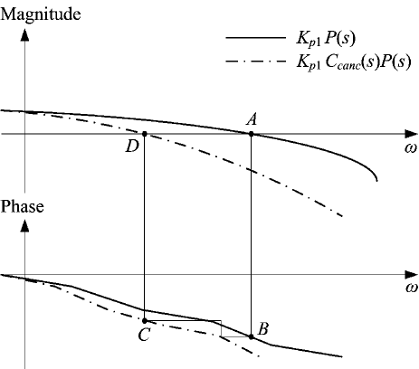
Figure 5: The design procedure for canceller to increase PM and keep the DC gain unchanged.

4 Experimental Results

A very linear NMP benchmark is needed for experimental verification of the results presented in previous section. Since most of the practical NMP systems are nonlinear to some extent, the circuit shown in Fig. 6 is proposed in this paper to be used as the NMP benchmark (the details of the buffers used in this figure are shown in Fig. 7). In this circuit assuming $R_{1}=R_{2}$, $C_{1}=C_{2}$, and $R_{4}=R_{5}=R_{6}=R_{7}$ the transfer function of system is calculated as the following

$$P(s)=\frac{V_{o}(s)}{V_{i}(s)}=\frac{1-R_{2}C_{2}s}{(1+R_{2}C_{2}s)(1+R_{3}C_{3}s)},$$ (4.1)

which has a NMP zero at $s=1/R_{2}C_{2}$ and two stable poles at $s=-1/R_{2}C_{2}$ and $s=-1/R_{3}C_{3}$. Note also that the DC gain of this system is equal to unity. One advantage of this benchmark system is that the location of its NMP zero, as well as its DC gain and band-width, can easily be adjusted to the desired value by assigning suitable values to resistors and capacitors. The values of $R_{1}=R_{2}=R_{4}=R_{5}=R_{6}=R_{7}=1.5\mathrm{k}\Omega$, $C_{1}=C_{2}=330\mu$F, $R_{3}=820\Omega$, $C_{3}=200\mu$F, and the well-known op-amp LM741 are used in all simulations and the experimental setup of this paper (the op-amps are supplied with $\pm 10$ V DC voltage). The values assigned to resistors and capacitors are chosen such that, firstly, the time-constant of circuit be considerably larger than the time consumed by processor for digital emulation of canceller, and secondly, the circuit exhibits a considerable NMP behavior (which is identified by a large initial undershoot in the time domain step response). More precisely, since the canceller is realized through a very high order FIR filter (see the discussion below) the processor should be provided with enough time to complete the required calculations at each sampling period. Figure 8 shows the experimental pulse response of the circuit shown in Fig. 6 assuming the above mentioned values for resistors and capacitors. As it can be observed in this figure, step response of the open-loop system has about $46\%$ initial undershoot which is fairly close to the one predicted by Matlab simulation.

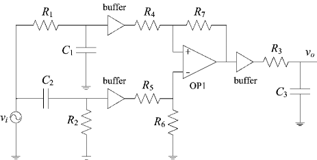
Figure 6: The proposed NMP benchmark circuit with transfer function $P(s)=V_{o}(s)/V_{i}(s)=\frac{1-R_{2}C_{2}s}{(1+R_{2}C_{2}s)(1+R_{3}C_{3}s)}$ (assuming $R_{1}=R_{2}$, $C_{1}=C_{2}$, and $R_{4}=R_{5}=R_{6}=R_{7}$).

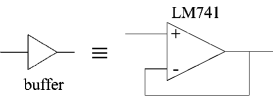
Figure 7: Details of the buffers used in Fig. 6.

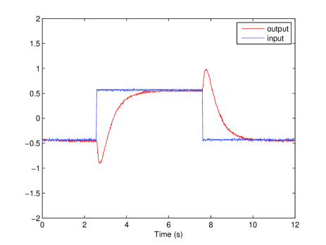
Figure 8: Experimental pulse response of the proposed NMP benchmark shown in Fig. 6.

At this time various methods are available for realization of simple fractional-order transfer functions like $PI^{\lambda}D^{\mu}$ or fractional-order lead-lag [19] (see also [20]-[24] for more information about the simulation and tuning of fractional-order PID controllers). But, according to the complexity of the proposed canceller these methods cannot be used for its realization. Hence, in order to realize the canceller first we calculate its impulse response $h_{canc}(t)$ by taking the inverse Laplace transform from $C_{canc}(s)$, that is

$$h_{canc}(t)=L^{-1}\left\{C_{canc}(s)\right\},$$ (4.2)

where according to (4.1) here we have

$$C_{canc}(s)=\frac{1}{1+(R_{2}C_{2}s)^{0.5}}.$$ (4.3)

The inverse Laplace transform in (4.2) can be calculated numerically using the Matlab function invlap.m which can be downloaded from Matworks website. After calculation of $h_{canc}(t)$, the equivalent discrete-time impulse response, $h_{canc}[n]$, can be calculated using the impulse-invariance method [18] as the following

$$h_{canc}[n]=Th_{canc}(nT),$$ (4.4)

where $T$ is the sampling period ($T$ is considered equal to 50 ms in this paper). Considering the fact that the power of $s$ in (4.3) is non-integer, it is expected that $h_{canc}(t)$ decays very slowly with time [15]. Hence, in order to realize $h_{canc}(t)$ with a high precision it is often needed to approximate it with a high-order FIR filter with impulse response $h_{canc}[n]$ as defined in (4.4). Figure 9 shows $h_{canc}(t)$ and $h_{canc}[n]$ for the system under consideration where $h_{canc}[n]$ is of length 100. Note that the DC gain of the canceller given in (4.3) is equal to unity, which implies that the impulse response of its discrete-time equivalent must satisfy the equality $\sum_{n=0}^{\infty}h_{canc}[n]=1$. But, this condition is violated in practice since both $h_{canc}(t)$ and $h_{canc}[n]$ are necessarily truncated for realization purposes, and moreover, the discontinuity of $h_{canc}(t)$ at $t=0$ is the source of some errors. Hence, in order to minimize the mismatch between theoretical and experimental results it is better to scale all samples of the truncated discrete-time impulse response $h_{canc}[n]$ such that their finite sum becomes equal to unity. For this purpose all samples of the $h_{canc}[n]$ calculated from (4.4) and shown in Fig. 9 are multiplied in 1.2 in the discussions of this paper. Then the difference equation of the FIR filter with truncated impulse response $h_{canc}[n]$ as described above is implemented using the ATmega16 AVR microcontroller. Finally, the digital output of this microcontroller is converted to analog using DAC08 A/D converter and the resulted analog output is connected to the input of benchmark circuit to form a closed-loop system. Note that in this experiment the command signal is directly entered to the input of microcontroller, and the subtractor and proportional controller of the feedback system are also realized using this microcontroller.

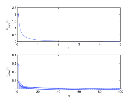
Figure 9: Impulse response of canceller, $h_{canc}(t)=L^{-1}\left\{C_{canc}(s)\right\}$, and its discrete-time impulse-invariance equivalent, $h_{canc}[n]=Th_{canc}(nT)$ ($T=50$ ms).

In the following discussion whenever we talk about $P(s)$ and $C_{canc}(s)$ equations (4.1) and (4.3) are under consideration, respectively.

Scenario 1: Design for the same DC gain. In this experiment we design a proportional controller and canceller such that both of the closed-loop systems (with and without using canceller) have the same DC gain while the PM in case of using canceller is much larger. For this purpose, without any loss of generality, first we choose $C(s)=K_{p}=1.07$ and $C_{canc}(s)=1$ in Fig. 1 to arrive at a feedback system whose PM is approximately equal to $60^{\circ}$ (see Fig. 10 for more details). Note that since in this case the DC gain of benchmark system is equal to unity, the DC gain of the resulted closed-loop system is equal to $1.07/(1+1.07)\approx 0.52$. Similarly, by choosing $C(s)=K_{p}=1.07$ in Fig. 1 and considering the canceller in the loop, the DC gain of the resulted closed-loop system with canceller is also equal to 0.52. Figure 10 shows the Nyquist plot of $K_{p}P(s)$ and $K_{p}C_{canc}(s)P(s)$ for $K_{p}=1.07$. As it can be observed in this figure, application of canceller changes the frequency response of open-loop system at higher frequencies without affecting its DC gain. Figure 11 shows the unit step response of the closed-loop systems with and without using canceller. This figure clearly shows that application of canceller considerably reduces the undershoot, overshoots, and settling time of the closed-loop step response. An explanation for the reduction of undershoot in the step response after applying the canceller can be found in [13]. The reason for considerable reduction of overshoot in the step response after applying the canceller is that partial cancellation highly increases the PM as it can be observed in Fig. 10. More precisely, according to Fig. 10 the PM before and after applying the canceller is approximately equal to $60^{\circ}$ and $175^{\circ}$, respectively. Decreasing the settling time in Fig. 11 after applying the canceller is a direct consequent of increasing the PM after cancellation. Note that all of the benefits observed in Fig. 11 are obtained only at the cost of slight increment in rise time, which is a direct consequent of decreasing the gain crossover frequency (as well as closed-loop bandwidth) after applying the canceller.

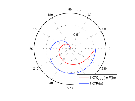
Figure 10: The Nyquist plot of open-loop system with and without using the canceller (proportional controller is applied). Both of the open-loop systems have the same DC gain.

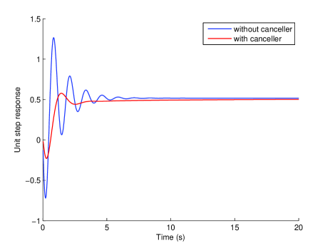
Figure 11: Simulation unit step responses of the closed-loop system with and without using canceller (a proportional controller with the gain 1.07 is applied in both cases).

The corresponding practical closed-loop step responses are shown in Fig. 12. The results shown in this figure are in a fair agreement with those obtained by numerical simulations and shown in Fig. 11. Note that there is some mismatch between the simulation and experimental results when the canceller is applied. This mismatch is caused because of truncation of the impulse response of canceller as well as its discrete-time realization.

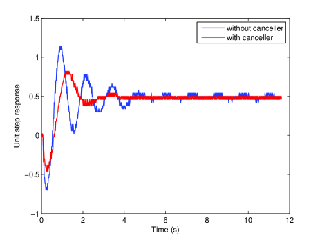
Figure 12: Experimental closed-loop unit step responses with and without using canceller (a proportional controller with the gain 1.07 is applied in both cases).

Scenario 2: Design for the same PM. Consider again the feedback system shown in Fig. 1 and suppose that once without using canceller and the other time at its presence we want to design the proportional controller such that the PM of the resulted closed-loop systems becomes equal to $60^{\circ}$, and then compare the performance of two systems. Similar to the discussions presented in Scenario 1, when the canceller is not applied this task can be done by choosing $K_{p}=1.07$. The Bode plot of the resulted open-loop system, $1.07P(s)$, is shown by the solid curve in Fig. 13. If in this case (i.e., assuming a proportional controller with the gain $K_{p}=1.07$ in the loop) we put the canceller given in (4.3) in series with $P(s)$ we arrive at a feedback system whose open-loop Bode plot is shown by the dash-dotted curve in Fig. 13. As it can be observed in this figure, application of canceller without increasing the gain of proportional controller highly increases the PM at the cost of decreasing the bandwidth of the closed-loop system. More precisely, application of canceller assuming $K_{p}=1.07$ leads to a feedback system with $PM\approx 175^{\circ}$. By a simple trial and error it can be easily verified that in case of using canceller by choosing $K_{p}=1.85$ the PM of the resulted feedback system becomes approximately equal to $60^{\circ}$ (see the dotted curve in Fig. 13). In other words, application of canceller makes it possible to use larger gains in the loop without any reduction of PM (note that possibility of using larger gains in the loop somehow compensates the reduction of closed-loop bandwidth after applying canceller). Figure 14 shows the Nyquist plots of $L_{1}(s)=1.07P(s)$ and $L_{2}(s)=1.85C_{canc}(s)P(s)$. As it can be observed in this figure, in both cases the PM is approximately equal to $60^{\circ}$ while the system with canceller has a considerably larger DC gain. The unit step response of the closed-loop system with and without using canceller obtained via numerical simulation is shown in Fig. 15. Note that the closed-loop system with canceller exhibits a smaller overshoot, undershoot, and steady-state error. The corresponding experimental closed-loop unit step responses are shown in Fig. 16. Although the experimental response with canceller has some differences with the one obtained from simulation, it still exhibits advantages compared to the one obtained without using it. More precisely, it can be observed in Fig. 16 that the closed-loop response with canceller has a considerably smaller undershoot, smaller settling time, and a smaller steady-state error compared to the one obtained without using it. The difference between practical and theoretical results at the presence of canceller is firstly because of truncation of the impulse response of canceller and secondly because of discretization which decreases the PM.

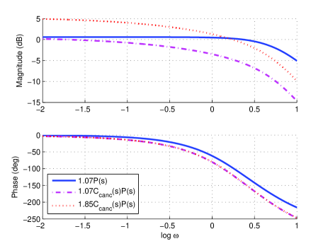
Figure 13: Bode plot of $1.07P(s)$ (PM=$60^{\circ}$, DC gain=1.07), $1.07C_{canc}(s)P(s)$ (PM=$175^{\circ}$, DC gain=1.07), and $1.85C_{canc}(s)P(s)$ (PM=$60^{\circ}$, DC gain=1.85).

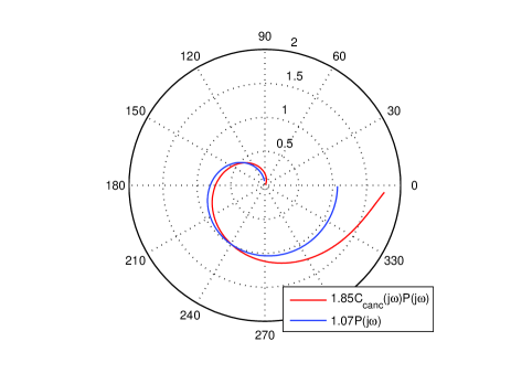
Figure 14: The Nyquist plot of open-loop system with and without using canceller (proportional controller is applied). Both of the open-loop systems have the same PM.

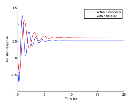
Figure 15: Simulation unit step responses of the closed-loop system with and without using canceller (the gain of proportional controller with and without using canceller is considered equal to 1.85 and 1.07, respectively.

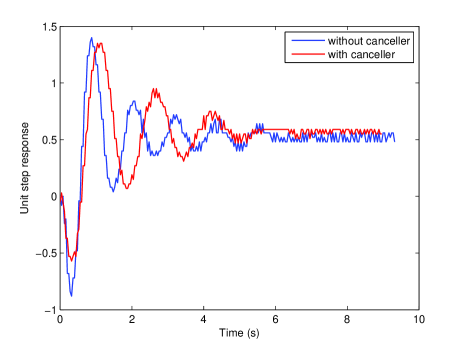
Figure 16: Experimental closed-loop unit step responses with and without using canceller (a proportional controller with the gain 1.07 is applied in both cases).

5 Conclusion

A method for partial cancellation of the NMP zero of a process located in feedback connection is presented in this paper. This partial cancellation is performed by means of a pre-compensator (canceller) located in series with the NMP process. Two methods for designing this pre-compensator are also proposed. In one of these methods the pre-compensator is designed such that the PM is increased while the open-loop DC gain remains unchanged. The other proposed method for designing pre-compensator can simultaneously increase the DC gain, PM, and GM of the open-loop system. Clearly, such a change in the open-loop system by means of pre-compensator can effectively facilitate the controller design procedure for NMP process and makes it possible to arrive at more effective closed-loop system.

The proposed methods for designing pre-compensator for partial cancellation of the NMP zero of process on the Riemann surface are also examined experimentally. For this purpose a very linear NMP benchmark circuit is proposed and the closed-loop system (including a proportional controller, pre-compensator, and the NMP process) is realized using a digital micro-controller. Experimental results show the high efficiency of the proposed cancellation strategies.

References

References

- Vakil et al. [2010] Vakil, M., Fotouhi, R. & Nikiforuk, P.N. (2010) On the zeros of the transfer function of flexible link manipulators and their non-minimum phase behaviour, P. I. Mech. Eng. C-J. Mec., 224 (10), 2083–2096.
- Benosman & Le Vey [2004] Benosman, M. & Le Vey, G. (2004) Control of flexible manipulators: A survey, Robotica, 22 (5), 533–545.
- Zhang et al. [2013] Zhang, Y., Liu, J. & Ma, X. (2013) Using RC type damping to eliminate right-half-plane zeros in high step-up DC-DC converter with diode-capacitor network, Proceedings of ECCE Asia, 3-6 June 2013, Melbourne, pp. 59-65.
- Chen et al. [2011] Chen, Z., Gao, W., Hu, J. & Ye, X. (2011) Closed-loop analysis and cascade control of a nonminimum phase boost converter, IEEE T. Power Electr., 26 (4), 1237–1252.
- Fischer [2013] Fischer, B. (2013) Reducing rotor speed variations of floating wind turbines by compensation of non-minimum phase zeros, IET Renew. Power Gen., 7 (4), 413–419.
- Chemori & Marchand [2008] Chemori, A. & Marchand, N. (2008) A prediction-based nonlinear controller for stabilization of a non-minimum phase PVTOL aircraft, Int. J. Robust Nonlin., 18 , 876–889.
- Åström et al. [2005] Åström, K.J., Klein, R.E. & Lennartsson, A. (2005) Bicycle dynamics and control: adapted bicycles for education and research, IEEE Contr. Syst. Mag., 25 (4), 26–47.
- Hoagg & Bernstein [2007] Hoagg, J.B. & Bernstein, D.S. (2007) Nonminimum-phase zeros-much to do about nothing, IEEE Contr. Syst. Mag., 27 (3), 45–57.
- Tofighi et al. [2015] Tofighi, S., Bayat, F. & Merrikh-Bayat, F. (2015) Robust feedback linearization of an isothermal continuous stirred tank reactor: mixed-sensitivity synthesis and DK-iteration approaches, T. I. Meas. Control, doi: 10.1177/0142331215603446.
- Aggarwal et al. [2013] Aggarwal, S., Garg, M. & Swarup, A. (2013) Design of feedback controller for non-minimum phase nano positioning system, Advanced Materials Letters, 4 (1), 31–34.
- Skogestad & Postlethwaite [2005] Skogestad, S. & Postlethwaite, I. (2005) Multivariable Feedback Control: Analysis and Design. 2nd Ed., New York: Wiley.
- Sidi [1997] Sidi, M. (1997) Gain-bandwidth limitations of feedback systems with non-minimum-phase plants, Int. J. Control, 67 (5), 731–743.
- Merrikh-Bayat [2013] Merrikh-Bayat, F. (2013) Fractional-order unstable pole-zero cancellation in linear feedback systems, J. Process Contr., 23 (6), 817–825.
- Åström & Hägglund [1995] Åström, K.J. & Hägglund, T. (1995) PID Controllers: Theory, Design, and Tuning. 2nd Ed., ISA.
- Podlubny [1999] Podlubny, I. (1999) Fractional Differential Equations. CA: Academic Press.
- Horwitz & Liao [1984] Horwitz, I. & Liao, Y.K. (1984) Limitations of non-minimum-phase feedback systems, Int. J. Control, 40 (5), 1003–1013.
- Seron et al. [1997] Seron, M.M., Braslavsky, J.H. & Goodwin, G.C. (1997) Fundamental Limitations in Filtering and Control. London: Springer-Verlag.
- Oppenheim & Schafer [2009] Oppenheim, A.V. & Schafer, R.W. (2009) Discrete-Time Signal Processing. 3rd Ed., Prentice-Hall.
- Podlubny et al. [2002] Podlubny, I., Petras, I., Vinagre, B.M., O’Leary, P. & Dorcak, L. (2002) Analogue realizations of fractional-order controllers, Nonlinear Dynam., 29 (4), 281–296.
- Merrikh-Bayat, F. & Karimi-Ghartemani, M. [2008] Merrikh-Bayat, F. & Karimi-Ghartemani, M. (2008) Method for designing stabilisers for minimum-phase fractional-order systems, IET Control Theory and Applications, 4 (1), 61–70.
- Merrikh-Bayat, F. [2011] Merrikh-Bayat, F. (2011) Efficient method for time-domain simulation of the linear feedback systems containing fractional order controllers, ISA Transactions, 50, 170–176.
- Merrikh-Bayat, F. [2012] Merrikh-Bayat, F. (2012) Rules for selecting the parameters of Oustaloup recursive approximation for the simulation of linear feedback systems containing controller, Commun. Nonlinear. Sci. Numer. Simulat., 17, 1852–1861.
- Merrikh-Bayat, F. [2012] Merrikh-Bayat, F. (2012) General rules for optimal tuning the controllers with application to first-order plus time delay processes, The Canadian Journal of Chemical Engineering, 90, 1400–1410.
- Merrikh-Bayat, F. et al. [2015] Merrikh-Bayat, F., Mirebrahimi, N., & Khalili, M.R. (2015) Discrete-time fractional-order PID controller: Definition, tuning, digital realization and some applications, International Journal of Control, Automation, and Systems, 13(1), 81–90.