Spaces of curves with constrained curvature
on hyperbolic surfaces

Abstract.

Let $S$ be a hyperbolic surface. We investigate the topology of the space of all curves on $S$ which start and end at given points in given directions, and whose curvatures are constrained to lie in a given interval $(\kappa_{1},\kappa_{2})$. Such a space falls into one of four qualitatively distinct classes, according to whether $(\kappa_{1},\kappa_{2})$ contains, overlaps, is disjoint from, or contained in the interval $[-1,1]$. Its homotopy type is computed in the latter two cases. We also study the behavior of these spaces under covering maps when $S$ is arbitrary (not necessarily hyperbolic nor orientable) and show that if $S$ is compact, then they are always nonempty.

0. Introduction

A curve on a surface $S$ is said to be regular if it has a continuous and nonvanishing derivative. Consider two such curves whose curvatures take values in some given interval, starting in the same direction (prescribed by a unit vector tangent to $S$) and ending in another prescribed direction. It is a natural problem to determine whether one curve can be deformed into the other while keeping end-directions fixed and respecting the curvature bounds. From another viewpoint, one is asking for a characterization of the connected components of the space of all such curves. More ambitiously, what is its homotopy or homeomorphism type? The answer can be unexpectedly interesting, and it is closely linked to the geometry of $S$. See the discussion below on some related results.

In this article this question is investigated when $S$ is hyperbolic, that is, a (possibly nonorientable) smooth surface endowed with a complete Riemannian metric of constant negative curvature, say, $-1$. It is well known that any such surface can be expressed as the quotient of the hyperbolic plane $\mathbb{H}^{2}$ by a discrete group of isometries. Thus any curve on $S$ can be lifted to a curve in $\mathbb{H}^{2}$ having the same curvature (at least in absolute value, if $S$ is nonorientable). As will be more carefully explained later, this implies that one can obtain a solution of the problem about spaces of curves on $S$ if one knows how to solve the corresponding problem in the hyperbolic plane for all pairs of directions.

Let $u,\,v\in UT\mathbb{H}^{2}$ (the unit tangent bundle of $\mathbb{H}^{2}$) be two such directions. Let $\mathscr{C}_{\kappa_{1}}^{\kappa_{2}}(u,v)$ be the set of all smooth regular curves on $\mathbb{H}^{2}$ whose initial (resp. terminal) unit tangent vectors equal $u$ (resp. $v$) and whose curvatures take values inside $(\kappa_{1},\kappa_{2})$, furnished with the $C^{\infty}$-topology. There are canonical candidates for the position of connected component of this space, defined as follows. Let

$$\operatorname{pr}\colon\widetilde{UT\mathbb{H}^{2}}\to UT\mathbb{H}^{2}$$

denote the universal cover. Fixing a lift $\tilde{u}$ of $u$, one obtains a map $\mathscr{C}_{\kappa_{1}}^{\kappa_{2}}(u,v)\to\operatorname{pr}^{-1}(v)$ by looking at the endpoint of the lift to the universal cover, starting at $\tilde{u}$, of curves in $\mathscr{C}_{\kappa_{1}}^{\kappa_{2}}(u,v)$. Since $\operatorname{pr}^{-1}(v)$ is discrete, this yields a decomposition of $\mathscr{C}_{\kappa_{1}}^{\kappa_{2}}(u,v)$ into closed-open subspaces.

More concretely, let $\gamma\colon[0,1]\to\mathbb{C}$ be a regular plane curve. An argument $\theta\colon[0,1]\to\mathbb{R}$ for $\gamma$ is a continuous function such that $\dot{}\gamma$ always points in the direction of $e^{i\theta}$; note that there are countably many such functions, which differ by multiples of $2\pi$. The total turning of $\gamma$ is defined as $\theta(1)-\theta(0)$. Because $\mathbb{H}^{2}$ is diffeomorphic to (an open subset of) $\mathbb{C}$, any regular curve in the former also admits arguments and a total turning. However, these have no geometric meaning since they depend on the choice of diffeomorphism (and subset). In any case, once such a choice has been made, it gives rise to the decomposition

(1) $$\mathscr{C}_{\kappa_{1}}^{\kappa_{2}}(u,v)=\bigsqcup_{\tau}\mathscr{C}_{\kappa_{1}}^{\kappa_{2}}(u,v;\tau),$$

where $\mathscr{C}_{\kappa_{1}}^{\kappa_{2}}(u,v;\tau)$ consists of those curves in $\mathscr{C}_{\kappa_{1}}^{\kappa_{2}}(u,v)$ which have total turning $\tau$, and $\tau$ runs over all valid total turnings, viz., those for which $v$ is parallel to $e^{i\tau}u$ (regarded as vectors in $\mathbb{C}$). The closed-open subspaces appearing on the right side of (1), which will be referred to as the canonical subspaces of $\mathscr{C}_{\kappa_{1}}^{\kappa_{2}}(u,v)$, are independent of the diffeomorphism: they are in bijective correspondence with the fiber $\operatorname{pr}^{-1}(v)$. If $\kappa_{1}=-\infty$ and $\kappa_{2}=+\infty$, so that no restriction is imposed on the curvature, then they are in fact precisely the components of $\mathscr{C}_{\kappa_{1}}^{\kappa_{2}}(u,v)$, and each of them is contractible. However, for general curvature bounds they may fail to be connected, contractible, or even nonempty. The possibilities depend above all upon the relation of $(\kappa_{1},\kappa_{2})$ to the interval $[-1,1]$.

The main results of the paper are (4.2), (5.1) and (6.5). The former two together assert the following.

Theorem.

Let $u,\,v\in UT\mathbb{H}^{2}$ and $\kappa_{1}<\kappa_{2}$.

1. If $(\kappa_{1},\kappa_{2})\subset[-1,1]$, then at most one of the canonical subspaces of $\mathscr{C}_{\kappa_{1}}^{\kappa_{2}}(u,v)$ is nonempty. This subspace is always contractible. Thus $\mathscr{C}_{\kappa_{1}}^{\kappa_{2}}(u,v)$ itself is either empty or contractible.

2. If $(\kappa_{1},\kappa_{2})$ is disjoint from $[-1,1]$, then infinitely many of the canonical subspaces are empty, and infinitely many are nonempty. The latter are all contractible.

If $(\kappa_{1},\kappa_{2})$ contains $[-1,1]$, then none of the canonical subspaces is empty. We conjecture that most are contractible, but finitely many of them may have the homotopy type of an $n$-sphere, for some $n\in\mathbb{N}$ depending upon the subspace. This conjecture is partly motivated by our knowledge of the homotopy type of the corresponding spaces of curves in the Euclidean plane, as determined in [36] and [37].

Finally, if $(\kappa_{1},\kappa_{2})$ overlaps $[-1,1]$, then infinitely many of the canonical subspaces are empty, and infinitely many are nonempty. Nevertheless, as in the previous case, simple examples (not discussed in this article) show that these subspaces may not be connected. We hope to determine the homotopy type in these two last cases in a future paper.

To state the third main result (6.5) referred to above, let $\mathscr{C}S_{\kappa_{1}}^{\kappa_{2}}(u,v)$ denote the space of curves on $S$ starting (resp. ending) in the direction of $u$ (resp. $v$) $\in UTS$ whose curvatures take values in $(\kappa_{1},\kappa_{2})$.

Theorem.

Let $S$ be any compact connected surface (not necessarily hyperbolic nor orientable). Then $\mathscr{C}S_{\kappa_{1}}^{\kappa_{2}}(u,v)\neq\emptyset$ for any choice of $\kappa_{1}<\kappa_{2}$ and $u,\,v\in UTS$.

Related results

A map $f\colon M^{m}\to N^{n}$ is said to be $k$-th order free if the $k$-th order osculating space of $f$ at any $p\in M$, which is generated by all (covariant) partial derivatives of $f$ at $p$ of order $\leq k$, has the maximum dimension, $d(k,m):={m+k\choose k}-1$, for all $p\in M$. Notice that a map is first-order free if and only if it is an immersion.

Although this definition of “freeness” uses covariant derivatives for simplicity, it is easy to avoid Riemannian metrics by using the language of jets. On the other hand, this formulation suggests the study of spaces of maps $f\colon M\to N$ satisfying more general differential inequalities, or partial differential relations. Various versions of Gromov’s h-principle (see [17] and [12]) are known which permit one to reduce the questions of existence, density and approximation of holonomic (i.e., true) solutions to a partial differential relation to the corresponding questions about formal (i.e., virtual) solutions; the latter are usually settled by invoking simple facts from homotopy theory.

It is known that if $n\geq d(k,m)+1$, or if $n=d(k,m)$ but $M$ is an open manifold, then the h-principle holds for $k$-th order free maps $M^{m}\to N^{n}$ (see [17], p. 9). In contrast, if $n$ equals the critical dimension $d(k,m)$ but $M$ is not open, then practically nothing is known regarding such maps. As an example, it is an open problem to decide whether a second-order free map $\mathbb{S}^{1}\times\mathbb{S}^{1}\to\mathbb{R}^{5}$ exists, cf. [12]. Indeed, it can be quite hard to disprove the validity of the h-principle even for the simplest differential relations.

In [35, 36, 37] and the current article we study spaces of curves whose curvature is constrained to a given interval $(\kappa_{1},\kappa_{2})$ on an elliptic, flat or hyperbolic surface. Such curves are holonomic solutions of a second-order differential relation on maps from a one-dimensional manifold (an interval, or a circle) to a two-dimensional manifold (the surface), so that we are in the critical dimension. In all of these cases we obtain some results on the homeomorphism type of the space of such curves, and in particular show that they do not abide to the h-principle. Other articles on the same topic, for curves in the Euclidean plane, include [5, 6, 11].

If $(\kappa_{1},\kappa_{2})=(-\infty,+\infty)$, then no condition is imposed on the curve except that it should be an immersion (i.e., regular). This problem was solved by H. Whitney [43] for closed curves in the plane and by S. Smale for closed curves on any manifold [39]. The case of immersions of higher-dimensional manifolds has also been elucidated, among others by S. Smale, R. Lashof and M. Hirsch in [19, 20, 23, 40, 41]. For results concerning the topology of spaces of immersions into space forms of nonpositive curvature having constrained principal curvatures (second fundamental form), see [46].

If $(\kappa_{1},\kappa_{2})=(0,+\infty)$, then we are asking that the curvature of the curve never vanish. This is equivalent to the requirement that it be second-order free. Such curves are also called nondegenerate or locally convex in the literature. Works on this problem include [21, 22, 24, 33]; see also [3]. More generally, $n$-th order free curves on $n$-dimensional manifolds have been studied by several authors over the years; we mention [1, 2, 13, 14, 15, 16, 25, 29, 34, 38, 44].

Finally, in another direction, there is a very extensive literature on applications of paths of constrained curvature in engineering and control theory. Perhaps the main problem in this regard is the determination of length-minimizing or other sort of optimal paths within this and related classes. We refer the reader to [4, 10, 26, 27, 28, 32] for further information and references.

Outline of the sections

After briefly introducing some notation and definitions, §1 begins with a discussion of curves of constant curvature $\kappa$ in the hyperbolic plane: circles ($\left|\kappa\right|>1$), horocycles ($\left|\kappa\right|=1$) and hypercircles ($\left|\kappa\right|<1$). Then a transformation is defined which takes a curve and shifts it by a fixed distance along the direction prescribed by its normal unit vectors. Its effect on the regularity and curvature of the original curve is investigated, and applied to reduce the dependence of the topology of $\mathscr{C}_{\kappa_{1}}^{\kappa_{2}}(u,v)$ to four real parameters, instead of the eight needed to specify $\kappa_{1},\,\kappa_{2},\,u$ and $v$.

In §2 the voidness of the canonical subspaces is discussed. It is proven that if $(\kappa_{1},\kappa_{2})$ is contained in $[-1,1]$, then the image of any curve in $\mathscr{C}_{\kappa_{1}}^{\kappa_{2}}(u,v)$ is the graph of a function when seen in an appropriate conformal model of the hyperbolic plane, which we call the Mercator model. In particular, at most one of its canonical subspaces is nonempty. If $(\kappa_{1},\kappa_{2})$ contains $[-1,1]$, then none of the canonical subspaces is empty. In the two remaining cases, there is a critical value $\tau_{0}$ for the total turning such that $\mathscr{C}_{\kappa_{1}}^{\kappa_{2}}(u,v;\tau)$ is nonempty for all $\tau\geq\tau_{0}$ and empty for all $\tau<\tau_{0}$ (or reversely, depending on whether $(\kappa_{1},\kappa_{2})$ contains points to the right or to the left of $[-1,1]$).

Section 3 explains how a curve of constrained curvature may also be regarded as a curve in the group of orientation-preserving isometries of $\mathbb{H}^{2}$ satisfying certain conditions. This perspective is sometimes useful.

In §4 it is shown that the nonempty canonical subspaces of $\mathscr{C}_{\kappa_{1}}^{\kappa_{2}}(u,v)$ are all contractible when $(\kappa_{1},\kappa_{2})$ is disjoint from $[-1,1]$. The idea is to parametrize all curves in such a subspace by the argument of its unit tangent vector when viewed as a curve in the half-plane model, and to take (Euclidean) convex combinations. The proof intertwines various Euclidean and hyperbolic concepts, and seems to be highly dependent on this particular model.

In the Mercator model $M$, any curve in $\mathscr{C}_{\kappa_{1}}^{\kappa_{2}}(u,v)$ may be parametrized as $x\mapsto(x,y(x))$ when $(\kappa_{1},\kappa_{2})$ is contained in $[-1,1]$, so the bounds on its curvature can be translated into two differential inequalities involving $\dot{y}$ and $\ddot{y}$, but not $y$ itself, because vertical translations are isometries of $M$. This allows one to produce a contraction of the space by working with the associated family of functions $\dot{y}$, as carried out in §5.

In §6 we define spaces of curves with constrained curvature on a general surface $S$, not necessarily hyperbolic, complete nor orientable, and explain how a Riemannian covering of $S$ induces homeomorphisms between spaces of curves on $S$ and on the covering space. We also show that if $S$ is compact then any such space is nonempty; this is also true in the Euclidean plane, but not in the hyperbolic plane, as mentioned previously. The section ends with a brief discussion of spaces of closed curves without basepoint conditions.

Several useful constructions, notably one which is essential to the proof of the main result of §5, may create discontinuities of the curvature, and thus lead out of the class of spaces $\mathscr{C}S_{\kappa_{1}}^{\kappa_{2}}(u,v)$ defined in §6. To circumvent this, the paraphernalia of $L^{2}$ functions is used in §7 to define another family of spaces, denoted $\mathscr{L}S_{\kappa_{1}}^{\kappa_{2}}(u,v)$, which are Hilbert manifolds. The curves in these spaces are regular but their curvatures are only defined almost everywhere. The main result of §7 states that the natural inclusion $\mathscr{C}S_{\kappa_{1}}^{\kappa_{2}}(u,v)\hookrightarrow\mathscr{L}S_{\kappa_{1}}^{\kappa_{2}}(u,v)$ is a homotopy equivalence with dense image. Sections 6 and 7 are independent of the other ones.

A few exercises are included in the article. These are never used in the main text, and their solutions consist either of straightforward computations or routine extensions of arguments presented elsewhere.

It is assumed that the reader is familiar with the geometry of the hyperbolic plane as discussed, for instance, in chapter 2 of [42], the expository article [9], chapter 7 of [7] or chapters 3–5 of [31].

1. Basic definitions and results

When speaking of the hyperbolic plane with no particular model in mind, we denote it by $\mathbb{H}^{2}$. The underlying sets of the (Poincaré) disk, half-plane and hyperboloid models are denoted by:

$$D =\big{\{}\,z\in\mathbb{C}\,\text{\ \large$:$\ }\,\left|z\right|<1\big{\}}\,;$$

$$H =\big{\{}\,z\in\mathbb{C}\,\text{\ \large$:$\ }\,\operatorname{Im}(z)>0\big{\}}\,;$$

$$L =\big{\{}\,(x_{0},x_{1},x_{2})\in\mathbb{E}^{2,1}\,\text{\ \large$:$\ }\,-x_{0}^{2}+x_{1}^{2}+x_{2}^{2}=-1\text{\ and\ }x_{0}>0\big{\}}\,.$$

The circle at infinity is denoted by $\mathbb{S}^{1}_{\infty}$ or $\partial\mathbb{H}^{2}$, the norm of a vector $v$ tangent to $\mathbb{H}^{2}$ by $\left|v\right|$, and the Riemannian metric by $\left\langle\ ,\ \right\rangle$. When working with $D$ or $H$, both $\mathbb{H}^{2}$ and its tangent planes are regarded as subsets of $\mathbb{C}$

In the disk and half-plane models, we will select the orientation which is induced on the respective underlying sets by the standard orientation of $\mathbb{C}$. In the hyperboloid model, a basis $(u,v)$ of a tangent plane is declared positive if $(u,v,e_{0})$ is positively oriented in $\mathbb{R}^{3}$; equivalently, the Lorentzian vector product $u\otimes v$ points to the exterior region bounded by $L$ (i.e., the one containing the light-cone).

Given a regular curve $\gamma\colon[0,1]\to\mathbb{H}^{2}$, its unit tangent is the map

$$\mathbf{t}=\mathbf{t}_{\gamma}\colon[0,1]\to UT\mathbb{H}^{2},\quad\mathbf{t}:=\frac{\dot{}\gamma}{\left|\dot{}\gamma\right|}.$$

Let $J\colon T\mathbb{H}^{2}\to T\mathbb{H}^{2}$ denote the bundle map (“multiplication by $i$”) which associates to $v\neq 0$ the unique vector $Jv$ of the same norm as $v$ such that $(v,Jv)$ is orthogonal and positively oriented. Then the unit normal to $\gamma$ is given by

$$\mathbf{n}=\mathbf{n}_{\gamma}\colon[0,1]\to UT\mathbb{H}^{2},\quad\mathbf{n}:=J\circ\mathbf{t}.$$

Assuming that $\gamma$ has a second derivative, its curvature is the function

(2) $$\kappa=\kappa_{\gamma}\colon[0,1]\to\mathbb{R},\quad\kappa:=\frac{1}{\left|\dot{}\gamma\right|}\Big{\langle}\frac{D\mathbf{t}}{dt},\mathbf{n}\Big{\rangle}=\frac{1}{\left|\dot{}\gamma\right|^{2}}\Big{\langle}\frac{D\dot{}\gamma}{dt},\mathbf{n}\Big{\rangle};$$

here $D$ denotes covariant differentiation (along $\gamma$). The hyperboloid model is usually the most convenient one for carrying out computations, since it realizes $\mathbb{H}^{2}$ as a submanifold of the vector space $\mathbb{E}^{2,1}$. For instance, the curvature of a curve $\gamma$ on $L$ is given by:

$$\kappa=\frac{\dot{\mathbf{t}}\cdot\mathbf{n}}{\left\|\dot{}\gamma\right\|}=\frac{\ddot{}\gamma\cdot\mathbf{n}}{\left\|\dot{}\gamma\right\|^{2}},$$

where $\cdot$ denotes the bilinear form on $\mathbb{E}^{2,1}$ and $\left\|\ \right\|^{2}$ is the associated quadratic form.

1.1 Definition (spaces of curves in $\mathbb{H}^{2}$).

Let $u,\,v\in UT\mathbb{H}^{2}$ and $\kappa_{1}<\kappa_{2}\in\mathbb{R}\cup\,\left\{\pm\infty\right\}\,$. Then $\mathscr{C}_{\kappa_{1}}^{\kappa_{2}}(u,v)$ (resp. $\bar{\mathscr{C}}_{\kappa_{1}}^{\kappa_{2}}(u,v)$) denotes the set of $C^{r}$ regular curves $\gamma\colon[0,1]\to\mathbb{H}^{2}$ satisfying:

1. $\mathbf{t}_{\gamma}(0)=u$ and $\mathbf{t}_{\gamma}(1)=v$;

2. $\kappa_{1}<\kappa_{\gamma}<\kappa_{2}$ (resp. $\kappa_{1}\leq\kappa_{\gamma}\leq\kappa_{2}$) throughout $[0,1]$.

This set is furnished with the $C^{r}$ topology, for some $r\geq 2$.

1.2 Definition (osculation).

Two curves $\gamma,\,\eta\colon[0,1]\overset{C^{2}}{\longrightarrow}S$ on a smooth surface $S$ will be said to osculate each other at $t=t_{0},\,t_{1}\in[0,1]$ if one may reparametrize $\gamma$, keeping $t_{0}$ fixed, so that

$$\gamma(t_{0})=\eta(t_{1})\in S,\quad\dot{}\gamma(t_{0})=\dot{\eta}(t_{1})\in TS\quad\text{and}\quad\ddot{}\gamma(t_{0})=\ddot{\eta}(t_{1})\in T(TS).$$

Remark.

Suppose that $S$ is oriented and furnished with a Riemannian metric. Then $\gamma$ and $\eta$ osculate each other at $t=t_{0},\,t_{1}$ if and only if

$$\gamma(t_{0})=\eta(t_{1}),\quad\mathbf{t}_{\gamma}(t_{0})=\mathbf{t}_{\eta}(t_{1})\quad\text{and}\quad\kappa_{\gamma}(t_{0})=\kappa_{\eta}(t_{1}).$$

1.3 Definition (circle, hypercircle, horocycle, ray).

A circle is the locus of all points a fixed distance away from a certain point in $\mathbb{H}^{2}$ (called its center). A hypercircle is one component of the locus of all points a fixed distance away from a certain geodesic in $\mathbb{H}^{2}$. A horocycle is a curve which meets all geodesics through a certain point of $\partial\mathbb{H}^{2}$ orthogonally. A ray is a distance-preserving map $\alpha\colon[0,+\infty)\to\mathbb{H}^{2}$; such a ray is said to emanate from $\alpha^{\prime}(0)\in UT\mathbb{H}^{2}$.

In order to understand the effect of a geometric transformation on a given curve, it is often sufficient to replace the latter by its family of osculating constant-curvature curves. Because the hyperbolic plane is homogeneous and isotropic, one can represent these in a convenient position in one of the models as a means of avoiding calculations.

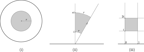
Figure 1. Computing the curvature of circles, hypercircles and horocycles through Gauss-Bonnet. The circle in (i) is represented in the disk model, while the hypercircle in (ii) and horocycles in (iii) are represented in the half-plane model.

1.4 Remark (constant-curvature curves).

Define an Euclidean circle to be either a line or a circle in $\mathbb{C}$; its center is taken to be $\infty$ if it is a line.

1. Circles, hypercircles and horocycles are the orbits of elliptic, hyperbolic and parabolic one-parameter subgroups of isometries, respectively. In particular, they have constant curvature.

2. In the models $D$ and $H$, a circle, horocycle or hypercircle appears as the intersection with $\mathbb{H}^{2}$ of an Euclidean circle which is disjoint, secant or (internally) tangent to $\partial\mathbb{H}^{2}$, respectively.

3. In the hyperboloid model, a circle, hypercircle or horocycle appears as a (planar) ellipse, hyperbola or parabola, respectively.

4. If all points of a circle lie at a distance $r>0$ from a certain point, then its curvature is given by $\pm\coth r$. Thus, all circles have curvature greater than $1$ in absolute value.

5. If all points of a hypercircle lie at a distance $r>0$ from a certain geodesic, then its curvature is given by $\pm\tanh r$. Thus, all hypercircles have curvature less than $1$ in absolute value.

6. The curvature of a horocycle equals $\pm 1$.

7. Circles, hypercircles, horocycles and their arcs account for all constant-curvature curves.

Assertions (d), (e) and (f) may be proved by mapping the curve through an isometry to the corresponding curve in Figure 1 and applying Gauss-Bonnet to the shaded region. The remaining assertions are also straightforward consequences of the transitivity of the group of isometries on $UT\mathbb{H}^{2}$.

In view of the sign ambiguity in the preceding formulas, it is desirable to redefine circles, hypercircles and horocycles not as subsets of $\mathbb{H}^{2}$, but as oriented curves therein. The radius $r\in\mathbb{R}$ of a circle or hypercircle is now defined so that its curvature $\kappa$ is given by

$$\kappa=\coth r\text{\quad or \quad}\kappa=\tanh r,$$

respectively. Then $\left|r\right|$ is the distance from the circle (resp. hypercircle) to the point (resp. geodesic) to which it is equidistant. Both expressions for the curvature apply to horocycles if these are regarded as circles/hypercircles of radius $\pm\infty$, a convention which we shall adopt. Observe that in all cases the sign of $r$ is the same as that of the curvature.

1.5 Remark (curvature and orientation).

Let the circle at infinity be oriented from left to right in $H$ and counter-clockwise in $D$. In either of these models (compare Figure 2):

1. If a hypercircle meets the circle at infinity at an angle $\alpha\in(0,\pi)$, then its curvature equals $\cos\alpha$. This follows from a reduction to the hypercircle depicted in Figure 1 (ii), with the indicated orientation, by expressing $r$ in terms of $\alpha$. More explicitly,

   $$r=\int_{\alpha}^{\frac{\pi}{2}}\frac{1}{\sin t}\,dt=-\log\tan\big{(}\tfrac{\alpha}{2}\big{)}\qquad(\alpha\in(0,\pi)),$$

   so that $\tanh r=\cos\alpha$.

2. If a circle is oriented (counter-)clockwise, then its curvature is less than $-1$ (greater than 1). This follows immediately from a reduction to Figure 1 (i).

3. Both preceding assertions can be extended to include horocycles. This follows by representing horocycles as circles tangent to the circle at infinity in the disk model.

Figure 2. Examples of curves of constant curvature in the disk model. Note that the sign of the curvature of a hypercircle need not agree with that of its Euclidean curvature.

1.6 Exercise (families of parallel hypercircles).

Let $p\neq q\in\mathbb{S}^{1}_{\infty}$ and $\kappa\in(-1,1)$. Then there exist exactly two hypercircles of curvature $\kappa$ through $p$ and $q$. Furthermore, in the models $D$ or $H$:

1. This pair of hypercircles is related by inversion in $\mathbb{S}^{1}_{\infty}$, and their Euclidean centers lie along the Euclidean perpendicular bisector $l$ of $\overline{pq}$.

Let $o$ and $o^{\prime}$ denote the Euclidean centers of $\mathbb{S}^{1}_{\infty}$ and the geodesic through the pair $p,\,q$, respectively.

1. Any point of $l$ except for $o$ and $o^{\prime}$ is the Euclidean center of a unique hypercircle of curvature in $(0,1)$ through $p$ and $q$. Describe its orientation in terms of the position of its center.

2. Using (1.5) (a), describe how its curvature changes as its center moves along $l$.

1.7 Definition (normal translation).

Let $\gamma\colon[0,1]\to\mathbb{H}^{2}$ be a regular curve and $\rho\in\mathbb{R}$. The normal translation $\gamma_{\rho}\colon[0,1]\to\mathbb{H}^{2}$ of $\gamma$ by $\rho$ is the curve given by

$$\gamma_{\rho}(t)=\exp_{\gamma(t)}(\rho\mathbf{n}(t))\qquad(t\in[0,1]),$$

where $\mathbf{n}$ is the unit normal to $\gamma$ and $\exp$ the (Riemannian) exponential map. In the hyperboloid model,

(3) $$\gamma_{\rho}(t)=\cosh\rho\,\gamma(t)+\sinh\rho\,\mathbf{n}(t)\qquad(t\in[0,1]).$$

Remark.

The unit tangent bundle of any smooth surface has a canonical contact structure (cf. [42], §3.7). A curve $\tilde{\gamma}$ on $UTS$ is Legendrian (with respect to this structure) if its projection to $S$ always points in the direction prescribed by $\tilde{\gamma}$. When $S$ is oriented, a (local) flow of contact automorphisms $\phi_{\rho}$ on $UTS$ can be defined by letting $\phi_{\rho}(u)$ be the parallel translation of $u$ along the geodesic perpendicular to $u$ by a signed distance of $\rho$ toward the left ($u\in UTS$, $\rho\in\mathbb{R}$). If $S$ is complete, $\phi_{\rho}$ is defined on all of $UTS$ for each $\rho\in\mathbb{R}$. The normal translation of $\gamma$ as defined in (1.7) is nothing but the projection to $S$ of $\phi_{\rho}(\mathbf{t}_{\gamma})$, in the special case where $S=\mathbb{H}^{2}$. As will be seen below, this operation may create or remove cusps.

1.8 Remark (normal translation of constant-curvature curves in $\mathbb{H}^{2}$).

Let $r,\,\rho\in\mathbb{R}$.

1. The normal translation by $\rho$ of a circle of radius $r$ is a circle of radius $r-\rho$, equidistant to the same point as the original circle.

2. The normal translation by $\rho$ of a hypercircle of radius $r$ is a hypercircle of radius $r-\rho$, equidistant to the same geodesic as the original hypercircle.

3. A normal translation of a horocycle is another horocycle, meeting orthogonally the same family of geodesics as the original horocycle.

More concisely, the normal translation of a constant-curvature curve of radius $r\in\mathbb{R}\cup\,\left\{\pm\infty\right\}\,$ by $\rho\in\mathbb{R}$ is a curve of the same type of radius $r-\rho$.

1. A normal translation of a hypercircle (resp. horocycle) meets $\partial\mathbb{H}^{2}$ in the same points (resp. point) as the original hypercircle (resp. horocycle), when represented in one of the models $D$ or $H$.

Once again, to prove these assertions one can use an isometry to represent the circle (hypercircle, horocycle) as in Figure 1, where they become trivial.

Notice also that $\rho$ goes from 0 to $2r$, the circle shrinks to a singularity ($\rho=r$) and then expands back to the original circle, but with reversed orientation ($\rho=2r$). When $\rho=r$ the hypercircle becomes the geodesic, and when $\rho=2r$ it becomes the other component of the locus of points at distance $\left|r\right|$ from the geodesic. This behavior is subsumed in the following result.

1.9 Lemma (normal translation of general curves).

Let $\gamma\colon[0,1]\to\mathbb{H}^{2}$ be smooth and regular,

$$\kappa_{-}=\min_{t\in[0,1]}\kappa(t)\quad\text{and}\quad\kappa_{+}=\max_{t\in[0,1]}\kappa(t).$$

Assume that $\coth\rho\notin[\kappa_{-},\kappa_{+}]$. Then:

1. The normal translation $\gamma_{\rho}$ is regular. In particular, $\gamma_{\rho}$ is regular for all $\rho$ in some open interval containing 0, and for all $\rho\in\mathbb{R}$ in case $[\kappa_{-},\kappa_{+}]\subset[-1,1]$.

2. $\mathbf{t}_{\gamma_{\rho}}\equiv\mathbf{t}_{\gamma}$ if these are regarded as taking values in $\mathbb{E}^{2,1}\supset L$.

Given $t\in[0,1]$, there exists a unique constant-curvature curve which osculates $\gamma$ at $\gamma(t)$. The radius of curvature $r_{\gamma}(t)$ of $\gamma$ at $\gamma(t)$ is defined as the radius of this osculating curve.

1. The radii of curvature of $\gamma_{\rho}$ and $\gamma$ are related by $r_{\gamma_{\rho}}=r_{\gamma}-\rho$.

2. The curvature of $\gamma_{\rho}$ is given by:

   $$\kappa_{\gamma_{\rho}}(t)=\begin{cases}\frac{1-\kappa_{\gamma}(t)\coth\rho}{\kappa_{\gamma}(t)-\coth\rho}&\text{if\quad$|{\kappa_{\gamma}(t)}|>1$;}\\ \frac{\kappa_{\gamma}(t)-\tanh\rho}{1-\kappa_{\gamma}(t)\tanh\rho}&\text{if\quad$|{\kappa_{\gamma}(t)}|<1$;}\\ \kappa_{\gamma}(t)&\text{if\quad$|{\kappa_{\gamma}(t)}|=1$. }\end{cases}$$

3. $(\gamma_{\rho})_{-\rho}=\gamma$.

Proof.

For (a) and (b), use (3). It is clear from the definition of “osculation” that if $\eta$ osculates $\gamma$ at $\gamma(t)$, then $\eta_{\rho}$ osculates $\gamma_{\rho}$ at $\gamma_{\rho}(t)$. Thus part (c) is a consequence of (1.8). Part (d) follows from the addition formulas for $\coth$ and $\tanh$, and part (e) is obvious. ∎

The topology of $\mathscr{C}_{\kappa_{1}}^{\kappa_{2}}(u,v)$ depends in principle upon eight real parameters: three for each of $u,\,v\in UT\mathbb{H}^{2}$, and two for the curvature bounds. This number can be halved by a suitable use of normal translations and isometries. In the sequel, two intervals are said to overlap if they intersect but neither is contained in the other one.

1.10 Proposition (parameter reduction).

Let $(\kappa_{1},\kappa_{2})\neq(-1,1)$ and $u,\,v,\,\bar{u}\in UT\mathbb{H}^{2}$ be given. Then there exist $\bar{v}\in UT\mathbb{H}^{2}$ and $\kappa_{0}$ such that $\mathscr{C}_{\kappa_{1}}^{\kappa_{2}}(u,v)$ is canonically homeomorphic to a space of the type listed in Table 1.

Case	$\mathscr{C}_{\kappa_{1}}^{\kappa_{2}}(u,v)$ homeomorphic to	Range of $\kappa_{0}$
$(\kappa_{1},\kappa_{2})$ contained in $[-1,1]$	$\mathscr{C}_{0}^{\kappa_{0}}(\bar{u},\bar{v})$	$(0,1]$
$(\kappa_{1},\kappa_{2})$ disjoint from $[-1,1]$	$\mathscr{C}_{\kappa_{0}}^{+\infty}(\bar{u},\bar{v})$	$[1,+\infty)$
$(\kappa_{1},\kappa_{2})$ overlaps $[-1,1]$	$\mathscr{C}_{\kappa_{0}}^{+\infty}(\bar{u},\bar{v})$	$[-1,1)$
$(\kappa_{1},\kappa_{2})$ contains $[-1,1]$	$\mathscr{C}_{-\kappa_{0}}^{+\kappa_{0}}(\bar{u},\bar{v})$	$(1,+\infty]$

Table 1. Reduction of the number of parameters controlling the topology of $\mathscr{C}_{\kappa_{1}}^{\kappa_{2}}(u,v)$, for $(\kappa_{1},\kappa_{2})\neq(-1,1)$.

The special role played by the interval $[-1,1]$ stems from the fact that any normal translation of a horocycle is a horocycle. The four classes listed in Table 1 are genuinely different in terms of their topological properties, as discussed in the introduction. In the only case not covered by (1.10), namely $(\kappa_{1},\kappa_{2})=(-1,1)$, given $u,\,v,\,\bar{u}$, one can find $\bar{v}$ such that $\mathscr{C}_{-1}^{+1}(u,v)$ is homeomorphic to $\mathscr{C}_{-1}^{+1}(\bar{u},\bar{v})$; for this it is sufficient to compose all curves in the former with an isometry taking $u$ to $\bar{u}$.

Proof.

The argument is similar for all four classes, so we consider in detail only the case where $(\kappa_{1},\kappa_{2})$ overlaps $[-1,1]$. Firstly, notice that composition with an orientation-reversing isometry switches the sign of the curvature of a curve. Therefore, by applying a reflection in some geodesic if necessary, it can be assumed that $-1\leq\kappa_{1}<1<\kappa_{2}$ (instead of $\kappa_{1}<-1<\kappa_{2}\leq 1$). Write $\kappa_{2}=\coth\rho_{2}$, $\kappa_{1}=\tanh\rho_{1}$ and $\kappa_{0}=\tanh(\rho_{1}-\rho_{2})$. Then normal translation by $\rho_{2}$ (i.e., the map $\gamma\mapsto\gamma_{\rho_{2}}$) provides a homeomorphism

$$\mathscr{C}_{\kappa_{1}}^{\kappa_{2}}(u,v)\to\mathscr{C}_{\kappa_{0}}^{+\infty}(u^{\prime},v^{\prime}),$$

where $u^{\prime}$ is obtained by parallel translating $u$ by a distance $\rho_{2}$ along the ray emanating from $Ju$, and similarly for $v^{\prime}$. The inverse of this map is simply normal translation by $-\rho_{2}$. All details requiring verification here were already dealt with in (1.9). Finally, post-composition of curves with the unique orientation-preserving hyperbolic isometry taking $u^{\prime}$ to $\bar{u}$ yields a homeomorphism

$$\mathscr{C}_{\kappa_{0}}^{+\infty}(u^{\prime},v^{\prime})\to\mathscr{C}_{\kappa_{0}}^{+\infty}(\bar{u},\bar{v}).$$

In the remaining cases, let $\rho_{i}$ denote the radius of a curve of constant curvature $\kappa_{i}$ ($i=1,2$). For the first class in the table, apply a reflection if necessary to ensure that $\kappa_{1}>-1$, then use normal translation by $\rho_{1}$. For the second class, reduce to the case where $\kappa_{1}\geq 1$ and apply normal translation by $\rho_{2}$. For the fourth class, apply a normal translation by $\frac{1}{2}(\rho_{1}+\rho_{2})$. In all cases, use an orientation-preserving isometry to adjust the initial unit tangent vector to $\bar{u}$. ∎

Remark.

The homeomorphism constructed in the proof of (1.10) operates on the curves in a given space by a composition of a normal translation and an isometry. It is “canonical” in the sense that these two transformations, as well as the values of $\kappa_{0}$ and $\bar{v}$, are uniquely determined by $\kappa_{1},\,\kappa_{2},\,u,\,v$ and $\bar{u}$. However, this does not preclude the existence of some more complicated homeomorphism between spaces in the second column of Table 1.

1.11 Exercise (extension of (1.10)).

Let $(\kappa_{1},\kappa_{2})\neq(-1,1)$ and $u,\,v,\,\bar{u}\in UT\mathbb{H}^{2}$ be given. Use the argument above to prove:

1. If $(\kappa_{1},\kappa_{2})$ contains $[-1,1]$, then there exist $\kappa_{0}\in[-\infty,-1)$ and $\bar{v}\in UT\mathbb{H}^{2}$ such that

   $$\mathscr{C}_{\kappa_{1}}^{\kappa_{2}}(u,v)\approx\mathscr{C}_{\kappa_{0}}^{+\infty}(\bar{u},\bar{v}).$$

2. If $-1<\kappa_{1}<\kappa_{2}<1$, then there exist $\kappa_{0}\in(0,1)$ and $\bar{v}\in UT\mathbb{H}^{2}$ such that

   $$\mathscr{C}_{\kappa_{1}}^{\kappa_{2}}(u,v)\approx\mathscr{C}_{-\kappa_{0}}^{+\kappa_{0}}(\bar{u},\bar{v}).$$

   Note that the hypothesis here is more restrictive than in the first case of the table.

2. Voidness of the canonical subspaces

The purpose of this section is to discuss which of the canonical subspaces of $\mathscr{C}_{\kappa_{1}}^{\kappa_{2}}(u,v)$ are empty. In the sequel $\mathscr{C}_{\kappa_{1}}^{\kappa_{2}}(u,\cdot)$ (resp. $\bar{\mathscr{C}}_{\kappa_{1}}^{\kappa_{2}}(u,\cdot)$) denotes the space obtained from (1.1) by omitting the restriction that $\mathbf{t}_{\gamma}(1)=v$.

2.1 Lemma (attainable endpoints).

If at least one $\left|\kappa_{i}\right|>1$, then $\mathscr{C}_{\kappa_{1}}^{\kappa_{2}}(u,v)\neq\emptyset$ for all $u,v\in UT\mathbb{H}^{2}$.

Proof.

By symmetry, we may assume that $\kappa_{2}>1$. Further, using normal translation by $\rho_{2}=\operatorname{arccoth}\kappa_{2}$, we reduce to the case where $\kappa_{2}=+\infty$. Let $q\in\mathbb{H}^{2}$ and $x\in UT\mathbb{H}^{2}_{q}$ be arbitrary. Consider the map

$$F_{x}\colon\mathscr{C}_{\kappa_{1}}^{+\infty}(x,\cdot)\to UT\mathbb{H}^{2},\quad F_{x}(\gamma)=\mathbf{t}_{\gamma}(1).$$

It is not hard to see that this map is open; cf.  (7.4). We begin by proving that $\operatorname{Im}(F_{x})\supset UT\mathbb{H}^{2}_{q}$. Since sufficiently tight circles are allowed, $x\in\operatorname{Im}(F_{x})$. Let $I\subset UT\mathbb{H}^{2}_{q}\cap\operatorname{Im}(F_{x})$ be an open interval about $x$. For each $y\in I$, let $R_{y}$ denote the elliptic isometry fixing $q$ and taking $x$ to $y$. Let

$$\phantom{\quad(y,\,z\in UT\mathbb{H}^{2}_{q})}\gamma_{y}\in\mathscr{C}_{\kappa_{1}}^{\kappa_{2}}(x,y)\quad\text{and}\quad\gamma_{z}\in\mathscr{C}_{\kappa_{1}}^{\kappa_{2}}(x,z)\quad(y,\,z\in UT\mathbb{H}^{2}_{q}).$$

Then the concatenation

$$\gamma_{y}\ast\big{(}R_{y}\circ\gamma_{z}\big{)}$$

starts at $x$ and ends at $dR_{y}(z)$. This curve may not have a second derivative at the point of concatenation, but it may be approximated by a smooth curve in $\mathscr{C}_{\kappa_{1}}^{\kappa_{2}}(x,R_{y}z)$. This shows that $\operatorname{Im}(F_{x})$ contains the interval $\big{\{}\,R_{y}z\,\text{\ \large$:$\ }\,y\in I\big{\}}\,$ about $z$ whenever it contains $z$. In turn, this implies that $\operatorname{Im}(F_{x})$ includes $UT\mathbb{H}^{2}_{q}$. Therefore, if $\operatorname{Im}(F_{u})$ contains any tangent vector $x$ based at $q$, it must also contain $UT\mathbb{H}^{2}_{q}\subset\operatorname{Im}(F_{x})$, by transitivity.

Now let $r:=\operatorname{arccoth}\kappa_{1}$ in case $\kappa_{1}>1$ and $r:=+\infty$ otherwise. If $\operatorname{Im}(F_{u})$ contains tangent vectors at $q$, then it also contains tangent vectors at $q^{\prime}$ for any $q^{\prime}\in B(q;2r)$, since $q^{\prime}$ can be reached from $q$ by the half-circle centered at the midpoint of the geodesic segment $qq^{\prime}$ of radius $\frac{1}{2}d(q,q^{\prime})<r$. We conclude that $\operatorname{Im}(F_{u})=UT\mathbb{H}^{2}$, that is, $\mathscr{C}_{\kappa_{1}}^{\kappa_{2}}(u,v)\neq\emptyset$ for all $v\in UT\mathbb{H}^{2}$. ∎

The converse of (2.1) is an immediate consequence of the following result; cf. also (2.3).

2.2 Lemma (unattainable endpoints).

Let $(\kappa_{1},\kappa_{2})\subset[-1,1]$ and $u\in UT\mathbb{H}^{2}$. The hypercircles (or horocycles) of curvature $\kappa_{1}$ and $\kappa_{2}$ tangent to $u$ divide $\mathbb{H}^{2}$ into four open regions. Any curve in $\mathscr{C}_{\kappa_{1}}^{\kappa_{2}}(u,\cdot)$ is confined to one of these regions $R$. Conversely, a point in $R$ can be reached by a curve of constant curvature in $\mathscr{C}_{\kappa_{1}}^{\kappa_{2}}(u,\cdot)$.

Proof.

The hypercircle of curvature $\frac{1}{2}(\kappa_{1}+\kappa_{2})$ tangent to $u$ meets $\partial\mathbb{H}^{2}$ at two points; let $R$ denote the open region whose closure contains the one point in $\partial\mathbb{H}^{2}$ towards which $u$ is pointing. Let $\gamma\in\mathscr{C}_{\kappa_{1}}^{\kappa_{2}}(u,\cdot)$. Comparison of the curvatures of $\gamma$ and those of the hypercircles bounding $R$ shows that $\gamma(t)\in R$ for sufficiently small $t>0$. Suppose for a contradiction that $\gamma$ reaches $\partial R$ for the first time at $t=T\in(0,1]$ at some point of the hypercircle $E$ of curvature $\kappa_{2}=\tanh r$. (In case $\kappa_{2}=1$, $E$ is a horocycle and $r=+\infty$.) The function

$$\delta\colon[0,T]\to\mathbb{R},\quad\delta(t)=d(\gamma(t),E)$$

vanishes at $0$ and $T$, hence it must attain its global maximum in $[0,T]$ at some $\tau\in(0,T)$, say $\delta(\tau)=\rho$. By (1.8), the normal translation of $E$ by $-\rho$ is a hypercircle (resp. horocycle) of curvature $\tanh(r+\rho)$, which must be tangent to $\gamma$ at $\gamma(\tau)$ because $\dot{}\delta(\tau)=0$. Since $\delta$ has a local maximum at $\tau$, comparison of curvatures yields that $\kappa_{\gamma}(\tau)\geq\tanh(r+\rho)>\kappa_{2}$, which is impossible.

The last assertion of the lemma holds because constant-curvature curves in $\mathscr{C}_{\kappa_{1}}^{\kappa_{2}}(u,\cdot)$ foliate $R$. ∎

Remark.

With the notation of (2.2), the image of any curve in $\bar{\mathscr{C}}_{\kappa_{1}}^{\kappa_{2}}(u,\cdot)$ is contained in $\bar{R}$ (see (1.1) for the definition of $\bar{\mathscr{C}}$). To prove this, let $\gamma$ be a curve in this space. If $\kappa_{\gamma}\equiv\kappa_{1}$ or $\kappa_{\gamma}\equiv\kappa_{2}$, then the image of $\gamma$ is entirely contained in $\partial R$. Otherwise, let $t_{0}<1$ be the infimum of all $t\in[0,1]$ such that $\kappa_{\gamma}(t)\in(\kappa_{1},\kappa_{2})$, and apply the argument of (2.2) to $\gamma|_{[t_{0},1]}$.

2.3 Corollary.

The spaces $\mathscr{C}_{\kappa_{1}}^{\kappa_{2}}(\cdot,\cdot)$ and $\bar{\mathscr{C}}_{\kappa_{1}}^{\kappa_{2}}(\cdot,\cdot)$ contain closed curves if and only if at least one $\left|\kappa_{i}\right|>1$.∎

2.4 Corollary.

Let $S$ be a hyperbolic surface. Then any closed curve whose curvature is bounded by 1 in absolute value is homotopically non-trivial (that is, it cannot represent the unit element of $\pi_{1}S$).

Proof.

Indeed, the previous corollary shows that the lift of such a curve to $\mathbb{H}^{2}$ cannot be closed. ∎

It will be convenient to introduce another model for $\mathbb{H}^{2}$, which bears some similarity to Mercator world maps.

2.5 Definition (Mercator model).

The underlying set of the Mercator model $M$ is $(0,\pi)\times\mathbb{R}$. Its metric is defined by declaring the correspondence

$$M\to H,\quad(x,y)\mapsto e^{y+ix}\qquad\big{(}x\in(0,\pi),~{}y\in\mathbb{R})$$

to be an isometry. Because this map is the composition of the complex exponential with a reflection in the line $y=x$, $M$ is conformal.

2.6 Remark (geometry of $M$).

It is straightforward to verify that in the Mercator model $M$:

1. Vertical lines $y\mapsto(x,y)$, or parallels, represent hypercircles of curvature $\cos x$, corresponding in $H$ to rays having $0\in H$ for their initial point (see (1.5) (a)). Horizontal segments, or meridians, are geodesics corresponding in $H$ to Euclidean half-circles centered at 0.

2. Vertical translations are hyperbolic isometries. The Riemannian metric $g$ is given by

   $$g_{(x,y)}=\frac{dx^{2}+dy^{2}}{\sin^{2}x}\qquad((x,y)\in M).$$

3. The Christoffel symbols are given by

   $$\Gamma_{ij}^{k}(x,y)=\begin{cases}0&\text{ if $i+j+k$ is odd;}\\ (-1)^{1+ij}\cot x&\text{ if $i+j+k$ is even.}\end{cases}$$

2.7 Lemma.

Let $(\kappa_{1},\kappa_{2})\subset[-1,1]$ and $u$ be the vector $1\in\mathbb{S}^{1}$ based at $\big{(}\frac{\pi}{2},0\big{)}\in M$. Then the image of any curve in $\mathscr{C}_{\kappa_{1}}^{\kappa_{2}}(u,\cdot)$ or $\bar{\mathscr{C}}_{\kappa_{1}}^{\kappa_{2}}(u,\cdot)$ is the graph of a function of $x$ when represented in $M$. Conversely, if $(\kappa_{1},\kappa_{2})\not\subset[-1,1]$, then there exist curves in these spaces which are not graphs.

Proof.

Suppose that $\gamma\in\bar{\mathscr{C}}_{\kappa_{1}}^{\kappa_{2}}(u,\cdot)$ is not the graph of function of $x$ when represented in $M$, i.e., it is tangent to a parallel $P_{1}$ at some time, say, $t=1$. Let $P_{0}$ be the parallel $x=\frac{\pi}{2}$, which is orthogonal to $\gamma$ at $t=0$ by hypothesis; note that $P_{0}$ is a geodesic. Let $L$ be the meridian through $\gamma(1)$, which is a geodesic orthogonal to both $P_{0}$ and $P_{1}$. Let $\gamma_{1}$ be the concatenation of $\gamma$ and its reflection in $L$ (with reversed orientation). Let $\gamma_{2}$ be the concatenation of $\gamma_{1}$ and its reflection in $P_{0}$ (again with reversed orientation). Then $\gamma_{2}$ is a closed curve, hence $(\kappa_{1},\kappa_{2})\not\subset[-1,1]$ by (2.3).

Conversely, if $(\kappa_{1},\kappa_{2})\not\subset[-1,1]$, then $\mathscr{C}_{\kappa_{1}}^{\kappa_{2}}(u,\cdot)$ contains circles, which are closed and hence not graphs. ∎

2.8 Proposition (attainable turnings).

Consider the decomposition (1) of $\mathscr{C}_{\kappa_{1}}^{\kappa_{2}}(u,v)$ into canonical subspaces.

1. If $(\kappa_{1},\kappa_{2})$ contains $[-1,1]$, then all of its canonical subspaces are nonempty.

2. If $(\kappa_{1},\kappa_{2})$ is contained in $[-1,1]$, then at most one canonical subspace is nonempty.

3. If $(\kappa_{1},\kappa_{2})$ overlaps or is disjoint from $[-1,1]$, then infinitely many of the canonical subspaces are nonempty, and infinitely many are empty.

Proof.

We split the proof into parts.

1. By (2.1), $\mathscr{C}_{\kappa_{1}}^{\kappa_{2}}(u,v)\neq\emptyset$. Since $(\kappa_{1},\kappa_{2})\supset[-1,1]$, we may concatenate a curve in this space with circles of positive or negative curvature, traversed multiple times, to attain any desired total turning.

2. By (1.10), we may assume that $u$ is the vector in the statement of (2.7). Then the assertion becomes an immediate consequence of the latter.

3. By (2.1), $\mathscr{C}_{\kappa_{1}}^{\kappa_{2}}(u,v)\neq\emptyset$. Because we may concatenate any curve in $\mathscr{C}_{\kappa_{1}}^{\kappa_{2}}(u,v)$ with a circle (of positive curvature if $\kappa_{1}>-1$ and of negative curvature if $\kappa_{2}<1$) traversed multiple times, $\mathscr{C}_{\kappa_{1}}^{\kappa_{2}}(u,v;\tau)\neq\emptyset$ for infinitely many values of $\tau$. The remaining assertion, that $\mathscr{C}_{\kappa_{1}}^{\kappa_{2}}(u,v;\tau)=\emptyset$ for infinitely many values of $\tau$, is a consequence of (2.10) (c) below.∎

2.9 Definition ($\alpha_{\pm}$).

Given a regular curve $\gamma\colon[0,1]\to\mathbb{H}^{2}$, define maps

$$\alpha_{\pm}\colon[0,1]\to\mathbb{S}^{1}_{\infty}$$

by letting $\alpha_{\pm}(t)$ be the point where the geodesic ray emanating from $\pm\mathbf{n}(t)$ meets $\mathbb{S}^{1}_{\infty}$.

2.10 Lemma.

Let $u,\,v\in UT\mathbb{H}^{2}$ be fixed.

1. Two curves $\gamma,\,\bar{}\gamma\in\mathscr{C}_{-\infty}^{+\infty}(u,v)$ lie in the same component of this space if and only if the associated maps $\alpha_{+},\,\bar{}\alpha_{+}\colon[0,1]\to\mathbb{S}^{1}_{\infty}$ defined in (2.9) have the same total turning.

2. If $\kappa_{\gamma}>-1$ everywhere, then $\alpha_{-}$ is monotone. Similarly, if $\kappa_{\gamma}<+1$, then $\alpha_{+}$ is monotone.

3. If $\kappa_{1}\geq-1$, then then there exists $\tau_{0}$ such that $\mathscr{C}_{\kappa_{1}}^{\kappa_{2}}(u,v;\tau)$ is empty for all $\tau<\tau_{0}$.

Proof.

It is clear that if $\gamma,\,\bar{}\gamma$ lie in the same component, then $\alpha_{+}\simeq\bar{}\alpha_{+}$ and $\alpha_{-}\simeq\bar{}\alpha_{-}$. Conversely, if $\gamma,\,\bar{}\gamma$ do not lie in the same component, then $\bar{}\gamma$ must be homotopic (through regular curves) to the concatenation of $\gamma$ with a circle traversed $n$ times, for some $n\neq 0$. This yields a homotopy between $\bar{}\alpha_{+}$ and $\alpha_{+}$ concatenated with a map of degree $n$.

For part (b), it suffices to approximate $\gamma$ by its osculating constant-curvature curve at each point. If such a curve is a circle, place its center at the origin in the disk model. If it is a hypercircle, regard it as an Euclidean ray in $H$.

Finally, (c) is a corollary of (a) and (b). ∎

2.11 Exercise.

Let $\gamma\colon[0,1]\to\mathbb{H}^{2}$ be a regular curve and $A_{\pm}(\gamma)\subset\mathbb{S}^{1}_{\infty}$ denote the images of $\alpha_{\pm}\colon[0,1]\to\mathbb{S}^{1}_{\infty}$.

1. Each of $A_{\pm}(\gamma)$ is a closed arc, which may be a singleton or all of $\mathbb{S}^{1}_{\infty}$.

2. Regard $\gamma$ as a curve in $H$, and let $\infty$ be the unique point of $\mathbb{S}^{1}_{\infty}$ not on the real line in this model. Then $\infty$ lies in the complement of $A_{+}(\gamma)\cup A_{-}(\gamma)$ if and only if $\mathbf{t}_{\gamma}$ is never horizontal.

3. Let $\eta$ be a horocycle of curvature $1$, tangent to $\mathbb{S}^{1}_{\infty}$ at $z$. Then $A_{+}(\eta)=\,\left\{z\right\}\,$ while $A_{-}(\eta)=\mathbb{S}^{1}_{\infty}\smallsetminus\,\left\{z\right\}\,$. What happens if the curvature of $\eta$ is $-1$? (Hint: reduce to the case where $z=\infty$.)

3. Frame and logarithmic derivative

The group $\operatorname{Iso}_{+}(\mathbb{H}^{2})$ of all orientation-preserving isometries of the hyperbolic plane acts simply transitively on $UT\mathbb{H}^{2}$. Therefore, an element $g$ of this group is uniquely determined by where it maps a fixed unit tangent vector $u_{0}$. This yields a correspondence between the two sets, viz., $g\leftrightarrow gu_{0}$. The frame

(4) $$\Phi=\Phi_{\gamma}\colon[0,1]\to\operatorname{Iso}_{+}(\mathbb{H}^{2})$$

of a regular curve $\gamma\colon[0,1]\to\mathbb{H}^{2}$ is the image of $\mathbf{t}_{\gamma}$ under this correspondence, and the logarithmic derivative $\Lambda=\Lambda_{\gamma}\colon[0,1]\to\textrm{L}(\operatorname{Iso}(\mathbb{H}^{2}))$ is its infinitesimal version. More precisely, $\Lambda$ is the translation of $\dot{\Phi}$ to the Lie algebra $\textrm{L}(\operatorname{Iso}(\mathbb{H}^{2}))$, defined by

(5) $$\dot{\Phi}(t)=TL^{\Phi(t)}(\Lambda(t))\quad(t\in[0,1]).$$

Here $TL^{\Phi(t)}$ denotes the derivative (at the identity) of left multiplication by $\Phi(t)$. Although $\Phi$ depends on the choice of $u_{0}$, $\Lambda$ does not.

To be explicit, let $S=\operatorname{diag}(-1,1,1)$,

$$\mathrm{O}_{2,1}=\big{\{}\,Q\in\mathrm{GL}_{3}(\mathbb{R})\,\text{\ \large$:$\ }\,Q^{t}SQ=S\big{\}}\,$$

be the group of isometries of $\mathbb{E}^{2,1}$ and

$$\mathrm{SO}^{+}_{2,1}=\big{\{}\,Q\in\mathrm{O}_{2,1}\,\text{\ \large$:$\ }\,\det(Q)=1\text{ and }Q(L)=L\big{\}}\,$$

be the connected component of the identity, which is isomorphic to $\operatorname{Iso}_{+}(\mathbb{H}^{2})$. The corresponding Lie algebra is

$$\mathfrak{so}_{2,1}=\big{\{}\,X\in\mathfrak{gl}_{3}(\mathbb{R})\,\text{\ \large$:$\ }\,X^{t}S+SX=0\big{\}}\,.$$

In the hyperboloid model $L$, the identification between $UT\mathbb{H}^{2}$ and $\operatorname{Iso}_{+}(\mathbb{H}^{2})$ takes the canonical form

(6) $$UTL_{p}\ni u\leftrightarrow\begin{pmatrix}|&|&|\\ p&u&p\otimes u\\ |&|&|\end{pmatrix}\in\mathrm{SO}^{+}_{2,1},$$

where $\otimes$ denotes the Lorentzian vector product in $\mathbb{E}^{2,1}$. (Recall that $u\otimes v=S(u\times v)$, where $\times$ denotes the usual vector product of vectors in $\mathbb{R}^{3}$.) Note that this correspondence is also of the form $gu_{0}\leftrightarrow g$ described above ($g\in\mathrm{SO}^{+}_{2,1}$), for $u_{0}=e_{1}=(0,1,0)\in UTL$.

3.1 Exercise (computations in $L$).

Let $\gamma\colon[0,1]\to L$ be smooth and regular.

1. Denoting differentiation with respect to the given parameter (resp. arc-length) by $\dot{}$ (resp. ^′):

   $$\mathbf{t}^{\prime}=\kappa\mathbf{n}+\gamma,\quad\mathbf{n}^{\prime}=-\kappa\mathbf{t}\quad\text{and}\quad\kappa=\mathbf{t}^{\prime}\cdot\mathbf{n}=\frac{1}{\left\|\dot{}\gamma\right\|}\dot{\mathbf{t}}\cdot\mathbf{n}=\frac{1}{\left\|\dot{}\gamma\right\|^{2}}\ddot{}\gamma\cdot\mathbf{n}=\frac{1}{\left\|\dot{}\gamma\right\|^{3}}\det(\gamma,\dot{}\gamma,\ddot{}\gamma).$$

   In these formulas $\gamma,\,\mathbf{t},\,\mathbf{n}$ are viewed as taking values in $\mathbb{E}^{2,1}$, $\cdot$ is the Lorentzian inner product and $\left\|\ \right\|^{2}$ the corresponding quadratic form.

2. The frame $\Phi\colon[0,1]\to\mathrm{SO}^{+}_{2,1}$ and logarithmic derivative $\Lambda\colon[0,1]\to\mathfrak{so}_{2,1}$ of $\gamma$ are given by

   $$\Phi=\begin{pmatrix}|&|&|\\ \gamma&\mathbf{t}&\mathbf{n}\\ |&|&|\end{pmatrix}\text{\quad and\quad}\Lambda=\left\|\dot{}\gamma\right\|\begin{pmatrix}0&1&0\\ 1&0&-\kappa\\ 0&\kappa&0\end{pmatrix}.$$

Similar formulas for the curvature in the disk and half-plane models are much more cumbersome. However, the frame and logarithmic derivative do admit comparatively simple expressions.

For concreteness, we choose the correspondence between $\mathrm{PSL}_{2}(\mathbb{R})=\operatorname{Iso}_{+}(H)$ and $UTH$ to be $M\leftrightarrow dM_{i}(1)$, where the latter denotes the image under the complex derivative $dM$ of the tangent vector $1\in\mathbb{C}$ based at $i\in H$. Similarly, we choose the correspondence between $\operatorname{Iso}_{+}(D)$ and $UTD$ to be $M\leftrightarrow dM_{0}(\frac{1}{2})$. Recall that $\operatorname{Iso}_{+}(D)$ consists of those Möbius transformations of the form

$$\qquad z\mapsto\frac{az+b}{\bar{b}z+\bar{a}},\quad\left|a\right|^{2}-\left|b\right|^{2}>0\quad(a,\,b\in\mathbb{C}).$$

3.2 Remark ($\Phi$ and $\Lambda$ in the models $D$ and $H$).

Denote elements of projective groups as matrices in square brackets, the absolute value of a complex number by $\left|\ \right|$ and, exceptionally, the norm of a vector tangent to $\mathbb{H}^{2}$ by $\left\|\ \right\|$.

1. Let $\gamma\colon[0,1]\to H$ be a smooth regular curve. Then $\Lambda\colon[0,1]\to\mathfrak{sl}_{2}({\mathbb{R}})$ is given by

   $$\Lambda=\frac{1}{2}\left\|\dot{}\gamma\right\|\begin{pmatrix}0&1+\kappa\\ 1-\kappa&0\end{pmatrix}$$

   and $\Phi\colon[0,1]\to\mathrm{PSL}_{2}(\mathbb{R})$ is given by

   $$\Phi=\begin{bmatrix}\operatorname{Im}(\gamma\bar{z})&\operatorname{Re}(\gamma\bar{z})\\ \operatorname{Im}(\bar{z})&\operatorname{Re}(\bar{z})\end{bmatrix},\quad\text{where $\frac{\mathbf{t}}{\left|\mathbf{t}\right|}=z^{2}\in\mathbb{S}^{1}$.}$$

2. Let $\gamma\colon[0,1]\to D$ be a smooth regular curve. Then $\Lambda\colon[0,1]\to\mathfrak{sl}_{2}(\mathbb{C})$ is given by

   $$\Lambda=\frac{1}{2}\left\|\dot{}\gamma\right\|\begin{pmatrix}i\kappa&1\\ 1&-i\kappa\end{pmatrix}$$

   and $\Phi\colon[0,1]\to\operatorname{Iso}_{+}(D)\subset\mathrm{PSL}_{2}(\mathbb{C})$ is given by

   $$\Phi=\begin{bmatrix}\phantom{\gamma}z&\gamma\bar{z}\\ \bar{}\gamma z&\phantom{\gamma}\bar{z}\end{bmatrix},\quad\text{where $\frac{\mathbf{t}}{\left|\mathbf{t}\right|}=z^{2}\in\mathbb{S}^{1}$.}$$

To establish the first formula, it suffices by (5) to consider the case the parameter is arc-length and $\Phi(s_{0})=I\in\mathrm{PSL}_{2}(\mathbb{R})$. Without trying to find an expression for $\Phi(s)$ itself, write

$$M^{s}:=\Phi(s)\in\mathrm{PSL}_{2}(\mathbb{R}),\quad M^{s}(z)=\frac{a(s)z+b(s)}{c(s)z+d(s)},\quad M^{s}(i)=\gamma(s)\in H,\quad dM^{s}_{i}=\mathbf{t}(s)\in\mathbb{C}.$$

(Here $dM^{s}$ denotes the complex derivative of $M^{s}$ as a map $\mathbb{C}\to\mathbb{C}$.) Differentiate with respect to $s$ at $s_{0}$ and express $\mathbf{t}^{\prime}(s_{0})$ in terms of $\frac{D\mathbf{t}}{ds}(s_{0})$ to determine $a^{\prime},b^{\prime},c^{\prime},d^{\prime}$ at $s_{0}$. The derivation of the formula for $\Lambda$ in (b) is analogous, and the expressions for $\Phi$ are obtained by straightforward computations.

A one-parameter group of hyperbolic isometries provides a foliation of $\mathbb{H}^{2}$ by its orbits, which are hypercircles by (1.4) (a). A regular curve $\gamma\colon[0,1]\to\mathbb{H}^{2}$ admits hyperbolic grafting if there exist some such group $G$ and $t_{0},t_{1}\in[0,1]$ such that $\mathbf{t}(t_{0})$ and $-\mathbf{t}(t_{1})$ are tangent to orbits of $G$.

3.3 Remark (hyperbolic grafting).

A regular curve $\gamma\colon[0,1]\to H$ admits hyperbolic grafting if and only if there exist $t_{0},t_{1}\in[0,1]$ such that $\Phi(t_{1})\Phi(t_{0})^{-1}$ has the form

$$\begin{bmatrix}r(1-\sin 2\theta)&-r\cos 2\theta\\ \cos 2\theta&-(1-\sin 2\theta)\end{bmatrix}=\begin{bmatrix}r(\cos\theta-\sin\theta)&-r(\cos\theta+\sin\theta)\\ \cos\theta+\sin\theta&\sin\theta-\cos\theta\end{bmatrix}\in\mathrm{PSL}_{2}(\mathbb{R})$$

for some $r>0$ and $\theta\in(0,\frac{\pi}{2})$.

For the proof, note that any two one-parameter groups of hyperbolic isometries are conjugate, hence $\Gamma$ may be taken as the group of positive homotheties centered at $0$. By homogeneity, it may also be assumed that $\mathbf{t}(t_{0})=i\in\mathbb{C}$ based at $i\in H$. Then $-\mathbf{t}(t_{1})=\operatorname{Im}(z)z$ if it is based at $z\in H$ and tangent to an orbit of $\Gamma$. The Möbius transformations $M\in\mathrm{PSL}_{2}(\mathbb{R})$ satisfying $dM_{i}(i)=-\operatorname{Im}(z)z$ ($z=re^{2i\theta}\in H$) admit the stated description.

4. The case where $(\kappa_{1},\kappa_{2})$ is disjoint from $[-1,1]$

4.1 Lemma.

In the disk and half-plane models, a curve whose (hyperbolic) curvature is everywhere greater than $1$ is locally convex from the Euclidean viewpoint, i.e., its total turning is strictly increasing.

Proof.

It suffices to prove this for curves of constant curvature greater than 1, because a general curve satisfying the hypothesis is osculated by curves of this type. In $D$ or $H$, such curves are represented as Euclidean circles traversed in the counterclockwise direction, hence they are locally convex. ∎

4.2 Theorem.

If $(\kappa_{1},\kappa_{2})$ is disjoint from $[-1,1]$, then each canonical subspace of $\mathscr{C}_{\kappa_{1}}^{\kappa_{2}}(u,v)$ is either empty or contractible.

Proof.

We will work in the half-plane model $H$ throughout the proof. Points and tangent vectors will thus be regarded as elements of $\mathbb{C}$. By (1.10), it may be assumed that $\kappa_{1}\geq 1$ and that $u$ is parallel to $1\in\mathbb{S}^{1}$. Let $\tau\in\mathbb{R}$ be a fixed valid total turning for curves in $\mathscr{C}_{\kappa_{1}}^{\kappa_{2}}(u,v)$, meaning that $e^{i\tau}$ is parallel to $v\in\mathbb{C}$.

Given $\gamma\in\mathscr{C}_{\kappa_{1}}^{\kappa_{2}}(u,v;\tau)$, let $\theta_{\gamma}\colon[0,1]\to[0,\tau]$ be the unique continuous function such that $\theta_{\gamma}(0)=0$ and

$$\frac{\mathbf{t}_{\gamma}(t)}{|\mathbf{t}_{\gamma}(t)|}=e^{i\theta_{\gamma}(t)}\text{ for all $t\in[0,1]$,}$$

where $\left|\ \right|$ denotes the usual absolute value of complex numbers. By (4.1), $\theta_{\gamma}$ is a diffeomorphism of $[0,1]$ onto $[0,\tau]$. Thus it may be used as a parameter for $\gamma$.

Now fix $\gamma_{0}\in\mathscr{C}_{\kappa_{1}}^{\kappa_{2}}(u,v;\tau)$ and set $\gamma_{1}:=\gamma$, both viewed as curves in $H$ and parametrized by the argument $\theta\in[0,\tau]$, as above. Define

$$\gamma_{s}(\theta)=(1-s)\gamma_{0}(\theta)+s\gamma_{1}(\theta)\in\mathbb{C}\quad(s\in[0,1],~{}\theta\in[0,\tau]).$$

Then each $\gamma_{s}\colon[0,\tau]\to H$ is a smooth curve satisfying $\mathbf{t}_{\gamma_{s}}(0)=u$ and $\mathbf{t}_{\gamma_{s}}(1)=v$. Moreover, it has the correct total turning $\tau$, since $\mathbf{t}_{\gamma_{s}}(\theta)$ is always parallel to $e^{i\theta}$. By (1.4) (g) and the definition of “osculation”, the constant-curvature curves osculating $\gamma$ from the Euclidean and hyperbolic viewpoints at any $\theta$ agree. Since $\kappa_{1}\geq 1$, they are both equal to a certain circle completely contained in $H$, traversed counterclockwise; compare (1.5) (b). Therefore the osculating constant-curvature curve to $\gamma_{s}$ at $\theta$ is another circle $C_{s}$, the corresponding convex combination of the osculating circles $C_{0}$ to $\gamma_{0}$ and $C_{1}$ to $\gamma_{1}$ at $\theta$ (see Figure 3). Let $y_{s}$ denote the $y$-coordinate of the Euclidean center of $C_{s}$ and $r_{s}$ its Euclidean radius ($s\in[0,1]$). More explicitly,

$$y_{s}=(1-s)y_{0}+sy_{1}\quad\text{and}\quad r_{s}=(1-s)r_{0}+sr_{1}.$$

The hyperbolic diameter $d_{s}$ of $C_{s}$ is given by

$$d_{s}=\log\bigg{(}\frac{y_{s}+r_{s}}{y_{s}-r_{s}}\bigg{)}.$$

Note that $y_{s}>r_{s}$, as this is true for $s=0,\,1$. Because

$$\phantom{\quad(i=0,1)}2\operatorname{arccoth}(\kappa_{2})<d_{i}<2\operatorname{arccoth}(\kappa_{1})\quad(i=0,1)$$

by hypothesis, a trivial computation shows that $d_{s}$ satisfies the same inequalities for all $s\in[0,1]$. Hence the curvature of $\gamma_{s}$ does indeed take values inside $(\kappa_{1},\kappa_{2})$, and $(\gamma,s)\mapsto\gamma_{s}$ defines a contraction of $\mathscr{C}_{\kappa_{1}}^{\kappa_{2}}(u,v;\tau)$. ∎

Figure 3. Proof of (4.2)

4.3 Corollary.

If $(\kappa_{1},\kappa_{2})$ is disjoint from $[-1,1]$, then $\mathscr{C}_{\kappa_{1}}^{\kappa_{2}}(u,v)$ is homeomorphic to the disjoint union of countably many copies of the separable Hilbert space.

Proof.

This is an immediate consequence of (2.8) (c), (4.2) and (7.8) (b). ∎

Remark.

It is interesting to note that the proof of (4.2) does not work in the disk model. To understand what could go wrong, consider the situation where $C_{0}$ and $C_{1}$ have the same radius and the midpoint of the segment joining their centers is the origin of $D$ (all concepts here being Euclidean). Then the hyperbolic radius of $C_{\frac{1}{2}}$ can be arbitrarily small compared to that of $C_{0}$ and $C_{1}$.

Remark.

The argument in the proof of (4.2) goes through without modifications to show that each component of $\bar{\mathscr{C}}_{\kappa_{1}}^{\kappa_{2}}(u,v)$ is contractible if $[\kappa_{1},\kappa_{2}]$ is disjoint from $[-1,1]$.

5. The case where $(\kappa_{1},\kappa_{2})\subset[-1,1]$

In this section we will work with the spaces $\mathscr{L}_{\kappa_{1}}^{\kappa_{2}}(u,v)$ which are introduced in §7. These are larger than $\mathscr{C}_{\kappa_{1}}^{\kappa_{2}}(u,v)$ in that they include regular piecewise $C^{2}$ curves. Our proof of (5.1) uses such curves and is therefore more natural in the former class. We recommend that the reader ignore the technical details for the moment and postpone a careful reading of §7. There is also a way to carry out the proof below in the setting of $\mathscr{C}_{\kappa_{1}}^{\kappa_{2}}(u,v)$: Whenever a discontinuity of the curvature arises, take an approximation by a smooth curve (which needs to be constructed); this path is more elementary but also cumbersome. The reader will notice that similar discussions appear in [33], [35] and [37].

Recall the Mercator model $M$ defined in (2.5). Suppose that $\gamma$ is a smooth regular curve in $M$ which can be written in the form

(7) $$\gamma\colon[a,b]\to M,\quad\gamma(x)=(x,y(x))$$

for some $[a,b]\subset(0,\pi)$; in other words, the image of $\gamma$ is the graph of a function $y(x)$. A straightforward computation using (2.6) shows that the curvature of $\gamma$ is then given by

(8) $$\kappa_{\gamma}=\frac{1}{\sqrt{1+\dot{y}^{2}}}\bigg{(}\frac{\ddot{y}\sin x}{1+\dot{y}^{2}}-\dot{y}\cos x\bigg{)}.$$

More important than this expression itself is the observation that it does not involve $y$, only its derivatives (because vertical translations are isometries of $M$). This can be exploited to express geometric properties of $\gamma$ solely in terms of the function $f=\dot{y}$, and in particular to prove the following.

5.1 Theorem.

If $(\kappa_{1},\kappa_{2})$ is contained in $[-1,1]$, then $\mathscr{C}_{\kappa_{1}}^{\kappa_{2}}(u,v)$ is either empty or contractible, hence homeomorphic to the separable Hilbert space.

Proof.

By (1.10), we can assume that $u$ is represented in $M$ as the vector $1\in\mathbb{S}^{1}$ based at $(\frac{\pi}{2},0)$. By (7.12), it suffices to prove that the Banach manifold $\mathscr{L}_{\kappa_{1}}^{\kappa_{2}}(u,v)$ is either empty or weakly contractible. Let

$$\mathbb{S}^{k}\to\mathscr{L}_{\kappa_{1}}^{\kappa_{2}}(u,v),\quad p\mapsto\gamma_{p}$$

be a continuous map. By (7.11), it can be assumed that each $\gamma_{p}$ is smooth. In particular, it is possible to choose $\bar{}\kappa_{2}<\kappa_{2}$ and $\bar{}\kappa_{1}>\kappa_{1}$ such that the curvatures of all the $\gamma_{p}$ take values inside $(\bar{}\kappa_{1},\bar{}\kappa_{2})$. By (2.7), any such curve $\gamma$ may be parametrized as in (7). The function $f=\dot{y}$ satisfies the following conditions, whose meaning will be explained below:

1. $f(a)=\alpha$ and $f(b)=\beta$.

2. $\int_{a}^{b}f(t)\,dt=A_{0}$.

3. $\psi_{\bar{}\kappa_{1}}(x,f(x))\leq\dot{f}(x)\leq\psi_{\bar{}\kappa_{2}}(x,f(x))$ for a.e. $x\in[a,b]$, where $\psi_{\kappa}\colon[a,b]\times\mathbb{R}\to\mathbb{R}$ is given by:

   $$\psi_{\kappa}(x,z)=\frac{1+z^{2}}{\sin x}\big{(}z\cos x+\kappa\sqrt{1+z^{2}}\big{)}\qquad(\kappa\in[\bar{}\kappa_{1},\bar{}\kappa_{2}],~{}x\in[a,b],~{}z\in\mathbb{R}).$$

In the present case, $a=\frac{\pi}{2}$ is the $x$-coordinate of $\gamma(a)=\big{(}\frac{\pi}{2},0\big{)}$ and $b$ is the $x$-coordinate of $\gamma(b)\in M\subset\mathbb{C}$. The real numbers $\alpha=0$ and $\beta$ in (i) are the slopes of $u$ and $v$ regarded as vectors in $\mathbb{C}$. Condition (ii) prescribes the $y$-coordinate of $\gamma(b)$. Finally, the inequalities in (iii) express the fact that the curvature of $\gamma$ takes values in $[\bar{}\kappa_{1},\bar{}\kappa_{2}]$; compare (8). Conversely, suppose that an absolutely continuous function $f\colon[a,b]\to\mathbb{R}$ satisfies (i)–(iii). If we set

$$y(x):=\int_{a}^{x}f(t)\,dt$$

and define $\gamma$ through (7), then $\gamma\in\mathscr{L}_{\kappa_{1}}^{\kappa_{2}}(u,v)$. Thus one can produce a contraction of the original family of curves by constructing a homotopy $(s,f)\mapsto f_{s}$ of the corresponding family of functions $f=f_{1}$, subject to the stated conditions throughout, with $f_{0}$ independent of $f$. This is what we shall now do.

For each $\kappa\in[\bar{}\kappa_{1},\bar{}\kappa_{2}]$, let $g_{\kappa}$ be the solution of the initial value problem

(9) $$\dot{g}(x)=\psi_{\kappa}(x,g(x)),\quad g(a)=\alpha,$$

where $\alpha$ and $\psi_{\kappa}$ are as in conditions (i) and (iii). Geometrically, the graph of $g$ is an arc of the hypercircle of curvature $\kappa$ with initial unit tangent vector $u$, represented in $M$. In particular, $g_{\kappa}$ is defined over all of $[a,b]$ by (2.7). Similarly, for each $\kappa\in[\bar{}\kappa_{1},\bar{}\kappa_{2}]$, let $h_{\kappa}$ be the solution of the initial value problem

$$\dot{h}(x)=\psi_{\kappa}(x,h(x)),\quad h(b)=\beta.$$

Geometrically, the graph of $h_{\kappa}$ is an arc of the hypercircle of curvature $\kappa$ whose final unit tangent vector is $v$. Although $h_{\kappa}$ is smooth, it is possible that it is not defined over all of $[a,b]$; if its maximal domain of definition is $(a^{\prime},b]$ for some $a^{\prime}>a$, then we extend $h_{\kappa}$ to a function $[a,b]\to\mathbb{R}\cup\,\left\{\pm\infty\right\}\,$ by setting it equal to $\lim_{x\to a^{\prime}{+}}h_{\kappa}(x)$ over $[a,a^{\prime}]$.

Using this geometric interpretation, it follows from (2.2) that

$$g_{\bar{}\kappa_{1}},\,h_{\bar{}\kappa_{1}}\leq f\leq g_{\bar{}\kappa_{2}},\,h_{\bar{}\kappa_{2}}.$$

Moreover, from the same result one deduces that

(10) $$g_{\kappa}(x)<g_{\kappa^{\prime}}(x)\ \ \text{for all\ \ $x>a$\ \ if\ \ $\kappa<\kappa^{\prime}$}.$$

For each $\lambda,\,\mu\in[\bar{}\kappa_{1},\bar{}\kappa_{2}]$, define $f_{(\lambda,\mu)}\colon[a,b]\to\mathbb{R}$ by

(11) $$f_{(\lambda,\mu)}(x)=\operatorname{median}\big{(}h_{\bar{}\kappa_{1}}(x)\,,\,g_{\lambda}(x)\,,\,f(x)\,,\,g_{\mu}(x)\,,\,h_{\bar{}\kappa_{2}}(x)\big{)}.$$

Notice first that this function does not take on infinite values, since $f,\,g_{\lambda},\,g_{\mu}$ are real functions. Similarly, since three of the functions above (namely, $f,\,g_{\lambda},\,g_{\mu}$) take the value $\alpha$ at $a$, and three of them (namely, $f,\,h_{\bar{}\kappa_{1}},\,h_{\bar{}\kappa_{2}}$) take the value $\beta$ at $b$, $f_{(\lambda,\mu)}$ automatically satisfies condition (i). It is easy to verify that it is Lipschitz and satisfies (iii) as well (see (5.2) below).

It remains to choose $(\lambda,\mu)$ appropriately to ensure that it satisfies condition (ii). Let

$$\kappa_{+}=\min \big{\{}\,\kappa\in[\bar{}\kappa_{1},\bar{}\kappa_{2}]\,\text{\ \large$:$\ }\,f(x)\leq g_{\kappa}(x)\text{ for all $x\in[a,b]$}\big{\}}\,,$$

$$\kappa_{-}=\max \big{\{}\,\kappa\in[\bar{}\kappa_{1},\bar{}\kappa_{2}]\,\text{\ \large$:$\ }\,g_{\kappa}(x)\leq f(x)\text{ for all $x\in[a,b]$}\big{\}}\,,$$

$$\Delta= \big{\{}\,(\lambda,\mu)\in[\kappa_{-},\kappa_{+}]\,\text{\ \large$:$\ }\,\lambda\leq\mu\big{\}}\,\text{\quad(cf.~{}Figure \ref{F:delta})}.$$

Figure 4. A diagram illustrating the triangle $\Delta$ in the $(\lambda,\mu)$-plane. The dashed segments are the intersections of $\Delta$ with the lines $\big{\{}\,(\lambda,\mu)\in\mathbb{R}^{2}\,\text{\ \large$:$\ }\,\mu-\lambda=s(\kappa_{+}-\kappa_{-})\big{\}}\,$ $(s\in[0,1])$.

Define $A\colon\Delta\to\mathbb{R}$ to be the area under the graph of $f_{(\lambda,\mu)}$:

$$A(\lambda,\mu)=\int_{a}^{b}f_{(\lambda,\mu)}(x)\mspace{2.0mu}dx.$$

Continuous dependence of the solutions of (9) on $\kappa$ implies that $A$ is a continuous function of $(\lambda,\mu)$. Moreover, from

$$h_{\bar{}\kappa_{1}},\,g_{\kappa_{-}}\leq f\leq g_{\kappa_{+}},\,h_{\bar{}\kappa_{2}},$$

one deduces that

$$f_{(\kappa_{-},\mu)}\leq f\leq f_{(\lambda,\kappa_{+})}$$

for all $\lambda,\,\mu\in[\kappa_{-},\kappa_{+}]$. Consequently, because the integral of $f$ equals $A_{0}$, for each $s\in[0,1]$ the set

$$\big{\{}\,(\lambda,\mu)\in\Delta\,\text{\ \large$:$\ }\,\mu-\lambda=s(\kappa_{+}-\kappa_{-})\text{\ and\ }A(\lambda,\mu)=A_{0}\big{\}}\,$$

is nonempty (see Figure 4). In fact, it consists of a unique point $(\lambda(s),\mu(s))$. To establish this, it suffices to show that $A(\lambda,\mu)$ is a strictly increasing function of both $\lambda$ and $\mu$. Now if

$$\kappa_{-}\leq\lambda<\lambda^{\prime}\leq\mu\leq\kappa_{+},$$

then the set of all $x\in[a,b]$ for which $g_{\lambda}(x)<f(x)<g_{\lambda^{\prime}}(x)$ is nonempty, by (10) and the choice of $\kappa_{\pm}$. Therefore $f_{(\lambda,\mu)}<f_{(\lambda^{\prime},\mu)}$ holds over a set of positive measure, while the nonstrict inequality holds everywhere by (10). This proves strict monotonicity with respect to $\lambda$; the argument for $\mu$ is analogous. Continuity of $A$ implies continuity of the curve $s\mapsto(\lambda(s),\mu(s))\in\Delta$ (which is depicted in bold in Figure 4). The functions

$$f_{s}\colon[a,b]\to\mathbb{R},\quad f_{s}=f_{(\lambda(s),\mu(s))}$$

satisfy all of conditions (i)–(iii) by construction, and they depend continuously on $f$ and $s$. Let $\kappa_{0}=\lambda(0)=\mu(0)$; then

$$f_{0}=\operatorname{median}\big{(}h_{\bar{}\kappa_{1}}\,,\,g_{\kappa_{0}}\,,\,h_{\bar{}\kappa_{2}}\big{)}.$$

By (10), there is at most one value of $\kappa\in[\bar{}\kappa_{1},\bar{}\kappa_{2}]$ for which the integral of $\operatorname{median}(h_{\bar{}\kappa_{1}}\,,\,g_{\kappa}\,,\,h_{\bar{}\kappa_{2}})$ equals $A_{0}$. This implies that $\kappa_{0}$, and hence $f_{0}$, is independent of $f$. Therefore $(f,s)\mapsto f_{s}$ is indeed a contraction. ∎

The following fact was used without proof above.

5.2 Lemma.

The function $f_{(\lambda,\mu)}$ of (11) is Lipschitz and satisfies (iii).

Proof.

More generally, let $\phi$ be the median of $\phi_{1},\dots,\phi_{2n+1}\colon[a,b]\to\mathbb{R}$. If each $\phi_{k}$ is $c$-Lipschitz, then $\phi$ is $c$-Lipschitz. Hence $\phi$ is absolutely continuous and its derivative exists a.e.. Furthermore, if $\phi$ and each $\phi_{k}$ are differentiable at $x$, then $\phi^{\prime}(x)=\phi_{k}^{\prime}(x)$ for some $k$ such that $\phi(x)=\phi_{k}(x)$. In particular, if each $\phi_{k}$ satisfies the inequalities in (iii) (with $\phi_{k}$ in place of $f$), then so does $\phi$.

The function $f_{(\lambda,\mu)}$ does not immediately conform to this situation because $h_{\bar{}\kappa_{i}}$ $(i=1,2)$ may take on infinite values. This can be circumvented by subdividing $[a,b]$ into at most three subintervals (where none, one or both of $h_{\bar{}\kappa_{i}}$ are infinite) and applying the preceding remarks. ∎

6. Spaces of curves with constrained curvature of class $C^{r}$

In this section we consider spaces of curves with constrained curvature on an arbitrary surface, not necessarily hyperbolic nor orientable. We study their behavior under covering maps and show that they are always nonempty if $S$ is compact; this should be contrasted with (2.1).

A surface is a smooth Riemannian 2-manifold. Given a regular curve $\gamma\colon[0,1]\to S$, its unit tangent $\mathbf{t}=\mathbf{t}_{\gamma}$ is the lift of $\gamma$ to the unit tangent bundle $UTS$ of $S$:

$$\mathbf{t}\colon[0,1]\to UTS,\quad\mathbf{t}(t)=\frac{\dot{}\gamma(t)}{\left|\dot{}\gamma(t)\right|}.$$

Now let an orientation of $TS_{\gamma(0)}$ be fixed. The unit normal to $\gamma$ is the map $\mathbf{n}=\mathbf{n}_{\gamma}\colon[0,1]\to UTS$ determined by the requirement that $(\mathbf{t}(t),\mathbf{n}(t))$ is an orthonormal basis of $TS_{\gamma(t)}$ whose parallel translation to $\gamma(0)$ (along the inverse of $\gamma$) is positively oriented, for each $t\in[0,1]$. Assuming $\gamma$ is twice differentiable, its curvature $\kappa=\kappa_{\gamma}$ is given by

(12) $$\kappa:=\frac{1}{\left|\dot{}\gamma\right|}\Big{\langle}\frac{D\mathbf{t}}{dt},\mathbf{n}\Big{\rangle}=\frac{1}{\left|\dot{}\gamma\right|^{2}}\Big{\langle}\frac{D\dot{}\gamma}{dt},\mathbf{n}\Big{\rangle}.$$

Here $D$ denotes covariant differentiation (along $\gamma$).

Remark.

If $S$ is nonorientable, it is more common to define the (unsigned) curvature of $\gamma\colon[0,1]\to S$ by

$$\kappa=\frac{1}{\left|\dot{}\gamma\right|}\left|\frac{D\mathbf{t}}{dt}\right|.$$

If $S$ is orientable, the usual definition coincides with (12), but $\mathbf{n}$ is defined by the condition that $(\mathbf{t}(t),\mathbf{n}(t))$ be positively oriented with respect to a specified orientation of $S$, rather than the parallel translation of an orientation of $TS_{\gamma(0)}$. These two definitions are equivalent, since an orientation of $TS_{\gamma(0)}$ determines an orientation of $S$ if the latter is orientable. The definition that we have chosen has the advantage of allowing arbitrary bounds for the curvature of a curve on a nonorientable surface, and in particular the concise formulation of (6.3) below.

A geometric interpretation for the curvature is the following: Let $v\colon[0,1]\to UTS$ be any smooth parallel vector field along $\gamma$, and let $\theta\colon[0,1]\to\mathbb{R}$ be a function measuring the oriented angle from $v(t)$ to $\mathbf{t}(t)$. Then a trivial computation shows that $\dot{\theta}=\kappa\left|\dot{}\gamma\right|$. In particular, the total curvature

$$\int_{0}^{1}\kappa(t)\left|\dot{}\gamma(t)\right|\,dt$$

of $\gamma$ equals $\theta(1)-\theta(0)$.

In all that follows, the curvature bounds $\kappa_{1}<\kappa_{2}$ are allowed to take values in $\mathbb{R}\cup\,\left\{\pm\infty\right\}\,$, $S$ denotes a surface and $u,\,v\in UTS$. Moreover, it is assumed that an orientation of $TS_{p}$, where $p$ is the basepoint of $u$, has been fixed.

6.1 Definition (spaces of $C^{r}$ curves).

Define $\mathscr{C}S_{\kappa_{1}}^{\kappa_{2}}(u,v)^{r}$ to be the set, endowed with the $C^{r}$ topology (for some $r\geq 2$), of all $C^{r}$ regular curves $\gamma\colon[0,1]\to S$ such that:

1. $\mathbf{t}_{\gamma}(0)=u$ and $\mathbf{t}_{\gamma}(1)=v$;

2. $\kappa_{1}<\kappa_{\gamma}(t)<\kappa_{2}$ for each $t\in[0,1]$.

Remark.

Of course, whether $S$ is orientable or not, the topological properties (or even the voidness) of $\mathscr{C}S_{\kappa_{1}}^{\kappa_{2}}(u,v)$ may be sensitive to the choice of orientation for $TS_{p}$. More precisely, if $\bar{S}$ denotes the same surface $S$ with the opposite orientation of $TS_{p}$, then $\mathscr{C}\bar{S}_{\kappa_{1}}^{\kappa_{2}}(u,v)=\mathscr{C}S_{-\kappa_{2}}^{-\kappa_{1}}(u,v)$.

It will follow from (7.12) that $r$ is irrelevant in the sense that different values yield spaces which are homeomorphic. Because of this, $\mathscr{C}S_{\kappa_{1}}^{\kappa_{2}}(u,v)^{r}$ is denoted simply by $\mathscr{C}S_{\kappa_{1}}^{\kappa_{2}}(u,v)$ in this section.

6.2 Lemma.

Define $\mathscr{C}S_{\kappa_{1}}^{\kappa_{2}}(u,\cdot)$ as in (6.1), except that no condition is imposed on $\mathbf{t}_{\gamma}(1)$, and similarly for $\mathscr{C}S_{\kappa_{1}}^{\kappa_{2}}(\cdot,v)$ and $\mathscr{C}S_{\kappa_{1}}^{\kappa_{2}}(\cdot,\cdot)$. Then:

1. $\mathscr{C}S_{\kappa_{1}}^{\kappa_{2}}(u,\cdot)$ and $\mathscr{C}S_{\kappa_{1}}^{\kappa_{2}}(\cdot,v)$ are contractible.

2. $\mathscr{C}S_{\kappa_{1}}^{\kappa_{2}}(\cdot,\cdot)$ is homotopy equivalent to $UTS$.

Proof.

By (7.8) (b), to prove that $\mathscr{C}S_{\kappa_{1}}^{\kappa_{2}}(u,\cdot)$ is contractible, it is actually sufficient to show that it is weakly contractible. Let

$$K\to\mathscr{C}S_{\kappa_{1}}^{\kappa_{2}}(u,\cdot),\quad p\mapsto\gamma^{p},$$

be a continuous map, where $K$ is a compact space. By a preliminary homotopy, each $\gamma^{p}$ may be reparametrized with constant speed. Let $\lambda(p)=\text{length}(\gamma^{p})$ and $0<\lambda<\inf_{p\in K}\lambda(p)$. The curves can be shrunk through the homotopy

$$(s,p)\mapsto\gamma_{s}^{p},\quad\gamma^{p}_{s}(t):=\gamma^{p}\Big{(}\lambda(p)^{-1}\big{[}(1-s)\lambda+s\lambda(p)\big{]}\mspace{2.0mu}t\Big{)}\quad(s,\,t\in[0,1],~{}p\in K)$$

so that all $\gamma_{0}^{p}$ have length $\lambda$, which can be chosen smaller than the injectivity radius of $S$ at the basepoint of $u$. Then each $\gamma_{0}^{p}$ is determined solely by its curvature, and conversely any function $\kappa\colon[0,1]\to(\kappa_{1},\kappa_{2})$ of class $C^{r-2}$ determines a unique curve of constant speed $\lambda$ in $S$ having $u$ for its initial unit tangent vector. But the set of all such functions is convex.

Reversal of orientation of curves yields a homeomorphism between and $\mathscr{C}S_{-\kappa_{2}}^{-\kappa_{1}}(-v,\cdot)$ and $\mathscr{C}S_{\kappa_{1}}^{\kappa_{2}}(\cdot,v)$, hence a space of the latter type is also contractible.

For (b), consider the map $f\colon UTS\to\mathscr{C}_{\kappa_{1}}^{\kappa_{2}}(\cdot,\cdot)$ which associates to $u$ the unique curve of constant curvature $\frac{1}{2}(\kappa_{1}+\kappa_{2})$ having $u$ for its initial unit tangent and length equal to half the injectivity radius of $S$ at the basepoint of $u$, parametrized with constant speed. Using the argument of the first paragraph, one deduces that $f$ is a weak homotopy inverse of

$$g\colon\mathscr{C}S_{\kappa_{1}}^{\kappa_{2}}(\cdot,\cdot)\to UTS,\quad g(\gamma)=\mathbf{t}_{\gamma}(0).$$

Therefore $\mathscr{C}_{\kappa_{1}}^{\kappa_{2}}(\cdot,\cdot)$ is homotopy equivalent to $UTS$, by (7.8) (b). ∎

6.3 Lemma.

Let $q\colon\tilde{S}\to S$ be a Riemannian covering (a covering map which is also a local isometry) and $u,\,v\in UTS$. Suppose that $dq\colon\big{(}T\tilde{S}_{\tilde{p}},\tilde{u}\big{)}\to\big{(}TS_{p},u\big{)}$ preserves the chosen orientation of these tangent planes. Then $\tilde{\gamma}\mapsto q\circ\tilde{\gamma}$ yields a homeomorphism

$$\bigsqcup_{\tilde{v}\in dq^{-1}(v)}\mathscr{C}\tilde{S}_{\kappa_{1}}^{\kappa_{2}}(\tilde{u},\tilde{v})\approx\mathscr{C}S_{\kappa_{1}}^{\kappa_{2}}(u,v).$$

Proof.

Let $\gamma\in\mathscr{C}S_{\kappa_{1}}^{\kappa_{2}}(u,v)$ and $\tilde{\gamma}\colon[0,1]\to\tilde{S}$ be its lift to $\tilde{S}$ starting at $\tilde{p}$. Since $dq$ is an isometry,

$$dq(\mathbf{t}_{\tilde{\gamma}})=\mathbf{t}_{\gamma}\quad\text{and}\quad dq(\mathbf{n}_{\tilde{\gamma}})=\pm\mathbf{n}_{\gamma}.$$

Moreover, $dq(\mathbf{n}_{\tilde{\gamma}}(0))=\mathbf{n}_{\gamma}(0)$ by the hypothesis regarding orientations, hence $dq(\mathbf{n}_{\tilde{\gamma}})=\mathbf{n}_{\gamma}$ by continuity. Now by (12), $\kappa_{\tilde{\gamma}}=\kappa_{\gamma}$. Therefore $\tilde{\gamma}\in\mathscr{C}\tilde{S}_{\kappa_{1}}^{\kappa_{2}}(\tilde{u},\tilde{v})$ for some lift $\tilde{v}$ of $v$. Conversely, if $\tilde{\gamma}\in\mathscr{C}\tilde{S}_{\kappa_{1}}^{\kappa_{2}}(\tilde{u},\tilde{v})$, then $\gamma=q\circ\tilde{\gamma}\in\mathscr{C}S_{\kappa_{1}}^{\kappa_{2}}(u,v)$ by the same reasons. Since projection and lift (starting at $\tilde{p}$) are inverse operations, the asserted homeomorphism holds. ∎

This result is especially useful when $S$ is a space form (e.g., a hyperbolic surface); for then $S$ is the quotient by a discrete group of isometries of the model simply-connected space of the same curvature, which is much more familiar. The lemma also furnishes a reduction to the orientable case by taking $\tilde{S}$ to be the two-sheeted orientation covering of $S$.

6.4 Exercise.

Suppose that $(\kappa_{1},\kappa_{2})$ is symmetric about 0. Then the conclusion of (6.3) holds regardless of whether $dq$ preserves orientation at $\tilde{p}$. (Hint: See the remark following (6.1).)

Remark.

If closed or half-open intervals were used instead in (6.1), then substantial differences would only arise in marginal cases. For instance, in the situation of (2.2), if $v$ is tangent to $\partial R$, then $\mathscr{C}_{\kappa_{1}}^{\kappa_{2}}(u,v)$ is empty, while $\bar{\mathscr{C}}_{\kappa_{1}}^{\kappa_{2}}(u,v)$ may not be. The original definition is more convenient to work with since the resulting spaces are Banach manifolds; compare Example 1.1 in [37].

6.5 Theorem.

Let $S$ be a compact connected surface. Then $\mathscr{C}S_{\kappa_{1}}^{\kappa_{2}}(u,v)\neq\emptyset$ for any choice of $\kappa_{1}<\kappa_{2}$ and $u,\,v\in UTS$.

Proof.

By passing to the orientation covering if necessary, it may be assumed that $S$ is oriented. Let $\kappa_{1}<\kappa_{2}$ be fixed. For $u,\,v\in UTS$, write $u\prec v$ if $\mathscr{C}S_{\kappa_{1}}^{\kappa_{2}}(u,v)\neq\emptyset$. Notice that $\prec$ is transitive: Given curves in $\mathscr{C}S_{\kappa_{1}}^{\kappa_{2}}(u,v)$ and $\mathscr{C}S_{\kappa_{1}}^{\kappa_{2}}(v,w)$, their concatenation starts at $u$ and ends at $w$; its curvature may fail to exist at the point of concatenation, but this can be fixed by taking a smooth approximation. Let

$$F_{u}=\big{\{}\,v\in UTS\,\text{\ \large$:$\ }\,u\prec v\big{\}}\,,\quad E_{u}=\big{\{}\,v\in UTS\,\text{\ \large$:$\ }\,u\prec v\textrm{ and }v\prec u\big{\}}\,.$$

It is clear from the definition that $F_{u}\neq\emptyset$ for all $u$, and that $F_{u}$ and $E_{u}$ are open subsets of $UTS$ (cf. (7.4)). Moreover, the family $(F_{u})_{u\in UTS}$ covers $UTS$. Indeed, given $v$, we can find $u$ such that $\mathscr{C}S_{-\kappa_{2}}^{-\kappa_{1}}(-v,-u)\neq\emptyset$. Reversing the orientation of a curve in the latter set, we establish that $\mathscr{C}S_{\kappa_{1}}^{\kappa_{2}}(u,v)\neq\emptyset$, that is, $v\in F_{u}$.

Since $UTS$ is compact, it can be covered by finitely many of the $F_{u}$. Let $UTS=F_{u_{1}}\cup\dots\cup F_{u_{m}}$ be a minimal cover. We claim that $m=1$.

Assume that $m>1$. If $u_{i}\prec u_{j}$ then $F_{u_{i}}\supset F_{u_{j}}$, and therefore by minimality $i=j$. Since $u_{i}\in UTS$ and $u_{i}\notin F_{u_{j}}$ for $j\neq i$, we deduce that $u_{i}\in F_{u_{i}}$ for each $i$. The open sets $E_{u_{i}}$ are thus nonempty and disjoint. On the other hand, every $F_{u_{i}}$ must intersect some $F_{u_{j}}$ with $j\neq i$, as $UTS$ is connected. Choose $i\neq j$ such that $F_{u_{i}}\cap F_{u_{j}}\neq\emptyset$. It is easy to see that $F_{u_{i}}\cap F_{u_{j}}$ must be disjoint from $E_{u_{i}}$. Thus, if $V$ is the interior of $F_{u_{i}}\smallsetminus E_{u_{i}}$, then $V\neq\emptyset$. We will obtain a contradiction from this. By definition, there exist $u_{\ast}\in E_{u_{i}}$, $v_{\ast}\in V$ and $\gamma_{\ast}\in\mathscr{C}S_{\kappa_{1}}^{\kappa_{2}}(u_{\ast},v_{\ast})$. Let $\gamma_{\ast}\colon[0,L]\to S$ be parametrized by arc-length and $\kappa_{\ast}\colon[0,L]\to(\kappa_{1},\kappa_{2})$ denote its curvature.

The tangent bundle $TS$ has a natural volume form coming from the Riemannian structure of $S$. A theorem of Liouville states that the geodesic flow preserves volume in $TS$. Since $S$ is oriented, given $\theta\in\mathbb{R}$ we may define a volume-preserving bundle automorphism on $UTS$ by $w\mapsto\cos\theta w+\sin\theta J(w)$ (where $J$ is “multiplication by $i$”). Let $Y_{0}$ and $Z$ be the vector fields on $UTS$ corresponding to the geodesic flow and to counterclockwise rotation, respectively. Then for any $\kappa\in\mathbb{R}$, the vector field $Y_{\kappa}=Y_{0}+\kappa Z$ defines a volume-preserving flow on $UTS$; the projections of its orbits on $S$ are curves parametrized by arc-length of constant curvature $\kappa$.

By definition, the open set $V$ is forward-invariant under each of these flows for $\kappa\in(\kappa_{1},\kappa_{2})$. Define a map $G\colon UTS\to UTS$ as follows: Given $u\in UTS$, $G(u)=\mathbf{t}_{\eta}(L)$, where $\eta\colon[0,L]\to S$ is the unique curve in $\mathscr{C}S_{\kappa_{1}}^{\kappa_{2}}(u,\cdot)$, parametrized by arc-length, whose curvature is $\kappa_{\ast}$. Then $G$ must be volume-preserving, $G(V)\subset V$, but there exists a neighborhood of $u_{\ast}$ contained in $E_{u_{i}}$ which is taken by $G$ to a neighborhood of $v_{\ast}$ contained in $V$, a contradiction.

We conclude that $m=1$, so that $UTS=F_{u_{1}}$. Furthermore, $F_{u_{1}}\smallsetminus E_{u_{1}}$ must have empty interior by the preceding argument. Hence $E_{u_{1}}$ is a dense open set in $UTS$. Let $u,\,v\in UTS$ be given. Since $F_{u}$ is open, there exists $v_{1}\in F_{u}\cap E_{u_{1}}$. Then $u\prec v_{1}$. Since $v_{1}\prec u_{1}$ and $u_{1}\prec v$, we deduce that $u\prec v$; in other words, $\mathscr{C}S_{\kappa_{1}}^{\kappa_{2}}(u,v)\neq\emptyset$. ∎

Spaces of closed curves without basepoints

Just as in algebraic topology one considers homotopies with and without basepoint conditions, one can also study the space of all smooth closed curves on $S$ with curvature in an interval $(\kappa_{1},\kappa_{2})$ but no restrictions on the initial and final unit tangents. Let this space be denoted by $\mathscr{C}S_{\kappa_{1}}^{\kappa_{2}}$. In some regards this class may seem more fundamental than its basepointed version, the class of spaces $\mathscr{C}S_{\kappa_{1}}^{\kappa_{2}}(u,v)$ considered thus far. However, in the Hirsch-Smale theory of immersions, such basepoint conditions arise naturally. For instance, thm. C of [39] states that $\mathscr{C}S_{-\infty}^{+\infty}(u,u)$ is (weakly) homotopy equivalent to the loop space $\Omega(UTS)(u)$ consisting of all loops in $UTS$ based at $u$. Moreover, even if one is interested only in closed curves, it is often helpful to study $\mathscr{C}S_{\kappa_{1}}^{\kappa_{2}}$ by lifting its elements to the universal cover of $S$, and these lifts need not be closed. A further point is provided by the following result. Recall that $UTS$ is diffeomorphic to $\mathbb{R}^{2}\times\mathbb{S}^{1}$ if $S=\mathbb{R}^{2}$ or $S=\mathbb{H}^{2}$, and to $\mathrm{SO}_{3}\approx\mathbb{R}\mathrm{P}^{3}$ if $S=\mathbb{S}^{2}$.

6.6 Lemma.

Let $S$ be a simply-connected complete surface of constant curvature and $u\in UTS$ be arbitrary. Then $\mathscr{C}S_{\kappa_{1}}^{\kappa_{2}}$ is homeomorphic to $UTS\times\mathscr{C}S_{\kappa_{1}}^{\kappa_{2}}(u,u)$.

Proof.

The group of orientation-preserving isometries of such a surface acts simply transitively on $UTS$. Given $v\in UTS$, let $g_{v}$ denote its unique element mapping $v$ to $u$. Define

$$f\colon\mathscr{C}S_{\kappa_{1}}^{\kappa_{2}}\to UTS\times\mathscr{C}_{\kappa_{1}}^{\kappa_{2}}(u,u),\quad f(\gamma)=(\mathbf{t}(0),g_{\mathbf{t}(0)}\circ\gamma).$$

This is clearly continuous, and so is its inverse, which is given by $(v,\eta)\mapsto g_{v}^{-1}\circ\eta$. ∎

Regard the elements of $\mathscr{C}S_{\kappa_{1}}^{\kappa_{2}}$ as maps $\mathbb{S}^{1}\to S$. There is a natural projection $\mathscr{C}S_{\kappa_{1}}^{\kappa_{2}}\to UTS$ taking a curve $\gamma\colon\mathbb{S}^{1}\to S$ to its unit tangent at $1\in\mathbb{S}^{1}$. This is a fiber bundle if $\kappa_{1}=-\infty$ and $\kappa_{2}=+\infty$ since $S$ is locally diffeomorphic to $\mathbb{R}^{2}$ and the group of diffeomorphisms of the latter acts transitively on $UT\mathbb{R}^{2}$. It may be a fibration in certain other special cases, as in the situation of (6.6), but in general this cannot be guaranteed. For instance, if $S=T^{2}$ is a flat torus, then the homotopy type of the fibers $\mathscr{C}S_{-1}^{+1}(u,u)$ of the map $\mathscr{C}S_{-1}^{+1}\to UTS$ is not locally constant; this follows from an example in the introduction of [36]. We believe that little is known about the topology of $\mathscr{C}S_{\kappa_{1}}^{\kappa_{2}}$ beyond what is implied by (6.6).

7. Spaces of curves with discontinuous curvature

Suppose that $\gamma\colon[0,1]\to S$ is a smooth regular curve and, as always, $TS_{\gamma(0)}$ has been oriented. Let $\sigma\colon[0,1]\to\mathbb{R}^{+}$ denote its speed $\left|\dot{}\gamma\right|$ and $\kappa$ its curvature. Then $\gamma$ and $\mathbf{t}=\mathbf{t}_{\gamma}\colon[0,1]\to UTS$ satisfy:

(13) $$\begin{cases}\dot{}\gamma=\sigma\mathbf{t}\\ \frac{D\mathbf{t}}{dt}=\sigma\kappa\mspace{2.0mu}\mathbf{n}\end{cases}\quad\text{and}\quad\mathbf{t}(0)=u\in UTS.$$

Thus, $\gamma$ is uniquely determined by $u$ and the functions $\sigma,\,\kappa$. One can define a new class of spaces by relaxing the conditions that $\sigma$ and $\kappa$ be smooth.

Let $h\colon(0,+\infty)\to\mathbb{R}$ be the diffeomorphism

$$h(t)=t-t^{-1}.$$

For each pair $\kappa_{1}<\kappa_{2}\in\mathbb{R}$, let $h_{\kappa_{1},\,\kappa_{2}}\colon(\kappa_{1},\kappa_{2})\to\mathbb{R}$ be the diffeomorphism

$$h_{\kappa_{1},\,\kappa_{2}}(t)=(\kappa_{1}-t)^{-1}+(\kappa_{2}-t)^{-1}$$

and, similarly, set

$$h_{-\infty,+\infty}\colon\mathbb{R}\to\mathbb{R},\qquad t\mapsto t$$

$$h_{-\infty,\kappa_{2}}\colon(-\infty,\kappa_{2})\to\mathbb{R},\qquad t\mapsto t+(\kappa_{2}-t)^{-1}$$

$$h_{\kappa_{1},+\infty}\colon(\kappa_{1},+\infty)\to\mathbb{R},\qquad t\mapsto t+(\kappa_{1}-t)^{-1}.$$

Notice that all of these functions are monotone increasing, hence so are their inverses. Moreover, if $\hat{\kappa}\in L^{2}[0,1]$, then $\kappa=h_{\kappa_{1},\kappa_{2}}^{-1}\circ\hat{}\kappa\in L^{2}[0,1]$ as well. This is obvious if $(\kappa_{1},\kappa_{2})$ is bounded, and if one of $\kappa_{1},\kappa_{2}$ is infinite, then it is a consequence of the fact that $h_{\kappa_{1},\kappa_{2}}^{-1}(t)$ diverges linearly to $\pm\infty$ with respect to $t$. In what follows, $\mathbb{L}$ denotes the separable Hilbert space $L^{2}[0,1]\times L^{2}[0,1]$.

7.1 Definition (admissible curve).

A curve $\gamma\colon[0,1]\to S$ is $(\kappa_{1},\kappa_{2})$-admissible if there exists $(\hat{}\sigma,\hat{}\kappa)\in\mathbb{L}$ such that $\gamma$ satisfies (13) with

(14) $$\sigma=h^{-1}\circ\hat{\sigma}\text{\quad and\quad}\kappa=\mspace{2.0mu}h^{-1}_{\kappa_{1},\,\kappa_{2}}\circ\hat{\kappa}.$$

When it is not important to keep track of the bounds $\kappa_{1},\kappa_{2}$, we will simply say that $\gamma$ is admissible.

The system (13) has a unique solution for any $(\hat{}\sigma,\hat{}\kappa)\in\mathbb{L}$ and $u\in UTS$. To see this, we use coordinate charts for $TS$ derived from charts for $S$ and apply thm. C.3 on p. 386 of [45] to the resulting differential equation, noticing that $S$ is smooth and $\sigma,\,\kappa\in L^{2}[0,1]\subset L^{1}[0,1]$. Furthermore, if we assume that $S$ is complete, then the solution is defined over all of $[0,1]$. The resulting maps $\gamma\colon[0,1]\to S$ and $\mathbf{t}\colon[0,1]\to TS$ are absolutely continuous (see p. 385 of [45]), and so is $\mathbf{n}$. Using that $\left\langle\mathbf{t},\mathbf{n}\right\rangle\equiv 0$ and differentiating, we obtain, in addition to (13), that

$$\frac{D\mathbf{n}}{dt}=-\sigma\kappa\mspace{2.0mu}\mathbf{t}\text{\quad and \quad}\left|\mathbf{t}(t)\right|=\left|\mathbf{n}(t)\right|=\left|u\right|=1\ \ \text{for all $t\in[0,1]$.}$$

Therefore, $\sigma=\left|\dot{}\gamma\right|$, $\mathbf{t}_{\gamma}=\mathbf{t}$ and $\mathbf{n}_{\gamma}=\mathbf{n}$. It is thus natural to call $\sigma$ and $\kappa$ the speed and curvature of $\gamma$, even though $\sigma,\,\kappa\in L^{2}[0,1]$.

Remark.

Although $\dot{}\gamma=\sigma\mathbf{t}$ is, in general, defined only almost everywhere on $[0,1]$, if we reparametrize $\gamma$ by arc-length then it becomes a regular curve, because $\gamma^{\prime}=\mathbf{t}$ is continuous. It is helpful to regard admissible curves simply as regular curves whose curvatures are defined a.e..

7.2 Definition.

For $u\in UTS$, let $\mathscr{L}S_{\kappa_{1}}^{\kappa_{2}}(u,\cdot)$ be the set of all $(\kappa_{1},\kappa_{2})$-admissible curves $\gamma\colon[0,1]\to S$ with $\mathbf{t}_{\gamma}(0)=u$.

If $S$ is complete, then this set is identified with $\mathbb{L}$ via the correspondence $\gamma\leftrightarrow(\hat{}\sigma,\hat{}\kappa)$, thus furnishing $\mathscr{L}S_{\kappa_{1}}^{\kappa_{2}}(u,\cdot)$ with a trivial Hilbert manifold structure. If $S$ is not complete, then $\mathscr{L}S_{\kappa_{1}}^{\kappa_{2}}(u,\cdot)$ is some mysterious open subset of $\mathbb{L}$. However, we still have the following.

7.3 Lemma.

For all $u\in UTS$, $\mathscr{L}S_{\kappa_{1}}^{\kappa_{2}}(u,\cdot)$ is homeomorphic to $\mathbb{L}$.

Proof.

The proof is almost identical to that of (6.2) (a). Given a family of curves indexed by a compact space, first reparametrize all curves by constant speed and shrink them to a common length $\lambda$ smaller than the injectivity radius of $S$ at the basepoint of $u$. Now each curve is completely determined by its curvature, and conversely any $L^{2}$-function $\hat{}\kappa\colon[0,1]\to\mathbb{R}$ determines a unique curve of constant speed $\lambda$ having $u$ for its initial unit tangent vector, via (14). But the set of all such functions is convex. Thus $\mathscr{L}S_{\kappa_{1}}^{\kappa_{2}}(u,\cdot)$ is weakly contractible, hence homeomorphic to $\mathbb{L}$ by (7.8) (a). ∎

7.4 Lemma.

Let $S$ be a surface and define $F\colon\mathscr{L}S_{\kappa_{1}}^{\kappa_{2}}(u,\cdot)\to UTS$ by $\gamma\mapsto\mathbf{t}_{\gamma}(1)$. Then $F$ is a submersion, and consequently an open map.

Proof.

The proof when $S=\mathbb{R}^{2}$ is given in [37], Lemma 1.5. The proof in the general case follows by considering Riemannian normal coordinates, which are flat at least to second order, in a neighborhood of the basepoint of $\mathbf{t}_{\gamma}(1)$. ∎

7.5 Definition (spaces of admissible curves).

Define $\mathscr{L}S_{\kappa_{1}}^{\kappa_{2}}(u,v)$ to be the subspace of $\mathscr{L}S_{\kappa_{1}}^{\kappa_{2}}(u,\cdot)$ consisting of all $\gamma$ such that $\mathbf{t}_{\gamma}(1)=v$.

It follows from (7.4) that $\mathscr{L}S_{\kappa_{1}}^{\kappa_{2}}(u,v)$ is a closed submanifold of codimension 3 in $\mathscr{L}S_{\kappa_{1}}^{\kappa_{2}}(u,\cdot)\approx\mathbb{L}$, provided it is not empty. We have already seen in (2.3) that such spaces may indeed be empty, but this cannot occur when $S$ is compact; cf. (6.5) and (7.10).

Relations between spaces of curves

If $(\kappa_{1},\kappa_{2})\subset(\bar{}\kappa_{1},\bar{}\kappa_{2})$ and $\gamma\in\mathscr{L}S_{\kappa_{1}}^{\kappa_{2}}(u,v)$, then we can also consider $\gamma$ as a curve in $\mathscr{L}S_{\bar{}\kappa_{1}}^{\bar{}\kappa_{2}}(u,v)$. However, the topology of the former space is strictly finer (i.e., has more open sets) than the topology induced by the resulting inclusion.

7.6 Lemma.

Let $(\kappa_{1},\kappa_{2})\subset(\bar{}\kappa_{1},\bar{}\kappa_{2})$, $S$ be a surface and $u\in UTS$. Then

(15) $$(\hat{}\sigma,\hat{}\kappa)\mapsto\big{(}\hat{}\sigma,h_{\bar{}\kappa_{1},\bar{}\kappa_{2}}\circ h_{\kappa_{1},\kappa_{2}}^{-1}\circ\hat{}\kappa\big{)}$$

defines a continuous injection $j\colon\mathscr{L}S_{\kappa_{1}}^{\kappa_{2}}(u,\cdot)\to\mathscr{L}S_{\bar{}\kappa_{1}}^{\bar{}\kappa_{2}}(u,\cdot)$. The actual curves on $S$ corresponding to these pairs are the same, but $j$ is not a topological embedding unless $\bar{}\kappa_{1}=\kappa_{1}$ and $\bar{}\kappa_{2}=\kappa_{2}$.

Proof.

It may be assumed that $S$ is oriented. The curve $\gamma$ corresponding to $(\hat{}\sigma,\hat{}\kappa)\in\mathscr{L}S_{\kappa_{1}}^{\kappa_{2}}(u,v)$ is obtained as the solution of (13) with

$$\sigma=h^{-1}\circ\hat{}\sigma\text{\quad and\quad}\kappa=h^{-1}_{\kappa_{1},\,\kappa_{2}}\circ\hat{}\kappa.$$

The curve $\eta$ corresponding to the right side of (15) in $\mathscr{L}S_{\bar{}\kappa_{1}}^{\bar{}\kappa_{2}}(u,\cdot)$ is the solution of (13) with

$$\sigma=h^{-1}\circ\hat{}\sigma\text{\quad and\quad}\kappa=h^{-1}_{\bar{}\kappa_{1},\,\bar{}\kappa_{2}}\circ\big{(}h_{\bar{}\kappa_{1},\bar{}\kappa_{2}}\circ h_{\kappa_{1},\kappa_{2}}^{-1}\circ\hat{}\kappa\big{)}=h^{-1}_{\kappa_{1},\,\kappa_{2}}\circ\hat{}\kappa.$$

By uniqueness of solutions, $\gamma=\eta$. In particular, $j$ is injective.

Set $g=h_{\bar{}\kappa_{1},\bar{}\kappa_{2}}\circ h_{\kappa_{1},\kappa_{2}}^{-1}$. Observe that

$$\lim_{t\to+\infty}g^{\prime}(t)=\begin{cases}1&\text{ if $\bar{}\kappa_{2}=\kappa_{2}$;}\\ 0&\text{ otherwise;}\end{cases}\qquad\lim_{t\to-\infty}g^{\prime}(t)=\begin{cases}1&\text{ if $\bar{}\kappa_{1}=\kappa_{1}$;}\\ 0&\text{ otherwise.}\end{cases}$$

Hence, $\left|g^{\prime}\right|$ is bounded over $\mathbb{R}$. Consequently, there exists $C>0$ such that

$$\left\|g\circ f_{1}-g\circ f_{2}\right\|_{2}\leq C\left\|f_{1}-f_{2}\right\|_{2}\ \ \text{for any $f_{1},\,f_{2}\in L^{2}[0,1]$.}$$

We conclude that $j\colon(\hat{}\sigma,\hat{}\kappa)\mapsto(\hat{}\sigma,g\circ\hat{}\kappa)$ is continuous.

Suppose now that $(\kappa_{1},\kappa_{2})\subsetneq(\bar{}\kappa_{1},\bar{}\kappa_{2})$. No generality is lost in assuming that $\kappa_{2}<\bar{}\kappa_{2}$. Let

$$m=g(0)\text{\ \ and \ \ }M=g(+\infty)=h_{\bar{}\kappa_{1},\bar{}\kappa_{2}}(\kappa_{2}).$$

Define a sequence of $L^{2}$ functions $\hat{}\kappa_{n}\colon[0,1]\to\mathbb{R}$ by:

$$\quad\hat{}\kappa_{n}(t)=\begin{cases}n&\text{ if $t\in\big{[}\frac{1}{2}-\frac{1}{2n}\,,\,\frac{1}{2}+\frac{1}{2n}\big{]}$;}\\ 0&\text{ otherwise. }\end{cases}\qquad(n\in\mathbb{N}^{+},~{}t\in[0,1]).$$

Since $g$ is the composite of increasing functions, $g(t)<g(+\infty)=M$ for any $t\in\mathbb{R}$. Therefore,

$$\left|g\circ\hat{}\kappa_{n}(t)-m\right|\begin{cases}\leq M-m&\text{ if\, $t\in\big{[}\frac{1}{2}-\frac{1}{2n}\,,\,\frac{1}{2}+\frac{1}{2n}\big{]}$;}\\ =0&\text{ otherwise}.\end{cases}$$

Hence, $\left\|\hat{\kappa}_{n}\right\|_{2}=\sqrt{n}\to+\infty$ as $n$ increases, while $\left\|g\circ\hat{}\kappa_{n}-m\right\|_{2}\leq n^{-\frac{1}{2}}(M-m)\to 0$. We conclude that $j$ is not a topological embedding. This argument may be modified to prove that $\mathscr{L}S_{\kappa_{1}}^{\kappa_{2}}(u,v)\hookrightarrow\mathscr{L}S_{\bar{}\kappa_{1}}^{\bar{}\kappa_{2}}(u,v)$ is likewise not an embedding for any $v$. ∎

7.7 Lemma.

Let $(\kappa_{1},\kappa_{2})\subset(\bar{}\kappa_{1},\bar{}\kappa_{2})$ and $u,\,v\in UTS$. Then

(16) $$j\colon\mathscr{C}S_{\kappa_{1}}^{\kappa_{2}}(u,v)^{r}\to\mathscr{L}S_{\bar{\kappa}_{1}}^{\bar{\kappa}_{2}}(u,v),\quad\gamma\mapsto(h\circ\left|\dot{}\gamma\right|\,,\,h_{\bar{}\kappa_{1}}^{\bar{}\kappa_{2}}\circ\kappa_{\gamma})$$

is a continuous injection, but not an embedding, for all $r\geq 2$. Moreover, the actual curve on $S$ corresponding to $j(\gamma)$ is $\gamma$ itself.

Proof.

The proof is very similar to that of (7.6). ∎

The following lemmas contain all the results on infinite-dimensional manifolds that we shall need.

7.8 Lemma.

Let $\mathscr{M},\,\mathscr{N}$ be (infinite-dimensional) Banach manifolds. Then:

1. If $\mathscr{M},\,\mathscr{N}$ are weakly homotopy equivalent, then they are in fact homeomorphic (diffeomorphic if $\mathscr{M},\,\mathscr{N}$ are Hilbert manifolds).

2. If the Banach manifold $\mathscr{M}$ and the finite-dimensional manifold $M$ are weakly homotopy equivalent, then $\mathscr{M}$ is homeomorphic to $M\times\mathbb{L}$; in particular, $\mathscr{M}$ and $M$ are homotopy equivalent.

3. Let $E$ and $F$ be separable Banach spaces. Suppose $i\colon F\to E$ is a bounded, injective linear map with dense image and $\mathscr{M}\subset E$ is a smooth closed submanifold of finite codimension. Then $\mathscr{N}=i^{-1}(\mathscr{M})$ is a smooth closed submanifold of  $F$ and $i\colon\mathscr{N}\to\mathscr{M}$ is a homotopy equivalence.

Proof.

Part (a) follows from thm. 15 in [30] and cor. 3 in [18]. For part (b), apply (a) to $\mathscr{M}$ and $\mathscr{N}=M\times\mathbb{L}$. Part (c) is thm. 2 in [8]. ∎

7.9 Lemma.

Let $\mathbb{L}$ be a separable Hilbert space, $D\subset\mathbb{L}$ a dense vector subspace, $L\subset\mathbb{L}$ a submanifold of finite codimension and $U$ an open subset of $L$. Then the set inclusion $D\cap U\to U$ is a weak homotopy equivalence.

Proof.

We shall prove the lemma when $L=h^{-1}(0)$ for some submersion $h\colon V\to\mathbb{R}^{n}$, where $V$ is an open subset of $\mathbb{L}$. This is sufficient for our purposes and the general assertion can be deduced from this by using a partition of unity subordinate to a suitable cover of $L$.

Let $T$ be a tubular neighborhood of $U$ in $V$ such that $T\cap L=U$. Let $K$ be a compact simplicial complex and $f\colon K\to U$ a continuous map. We shall obtain a continuous $H\colon[0,2]\times K\to U$ such that $H(0,a)=f(a)$ for every $a\in K$ and $H(\,\left\{2\right\}\,\times K)\subset D\cap U$. Let $e_{j}$ denote the $j$-th vector in the canonical basis for $\mathbb{R}^{n}$, $e_{0}=-\sum_{j=1}^{n}e_{j}$ and let $\Delta\subset\mathbb{R}^{n}$ denote the $n$-simplex $[e_{0},\dots,e_{n}]$. Let $[x_{0},x_{1},\dots,x_{n}]\subset T$ be an $n$-simplex and $\varphi\colon\Delta\to[x_{0},x_{1},\dots,x_{n}]$ be given by

$$\varphi\bigg{(}\sum_{j=0}^{n}s_{j}e_{j}\bigg{)}=\sum_{j=0}^{n}s_{j}x_{j},\text{\ \ where\ \ $\sum_{j=0}^{n}s_{j}=1$\ \ and\ \ $s_{j}\geq 0$\ \ for all\ \ $j=0,\dots,n$}.$$

We shall say that $[x_{0},x_{1},\dots,x_{n}]$ is neat if $h\circ\varphi\colon\Delta\to\mathbb{R}^{n}$ is an embedding and $0\in(h\circ\varphi)(\operatorname{Int}\Delta)$.

Given $p\in T$, let $dh_{p}$ denote the derivative of $h$ at $p$ and $N_{p}=\ker(dh_{p})$. Define $w_{j}\colon T\to\mathbb{L}$ by:

(17) $$w_{j}(p)=\big{(}dh_{p}|_{N_{p}^{\perp}}\big{)}^{-1}(e_{j})\quad(p\in T,~{}j=0,\dots,n).$$

Notice that $h\big{(}p+\sum_{j}\lambda_{j}w_{j}(p)\big{)}=h(p)+\sum_{j}\lambda_{j}e_{j}+o(\left|\lambda\right|)$ (for $\lambda=(\lambda_{0},\dots,\lambda_{n})$ and $p\in T$). Hence, using compactness of $K$, we can find $r,\varepsilon>0$ such that:

1. For any $p\in f(K)$, $[p+rw_{0}(p),\dots,p+rw_{n}(p)]\subset T$ and it is neat;

2. If $p\in f(K)$ and $\left|q_{j}-(p+rw_{j}(p))\right|<\varepsilon$ for each $j$, then $[q_{0},\dots,q_{n}]\subset T$ and it is neat.

Let $a_{i}$ ($i=1,\dots,m$) be the vertices of the triangulation of $K$. Set $v_{i}=f(a_{i})$ and

$$v_{ij}=v_{i}+rw_{j}(v_{i})\quad(i=1,\dots,m,~{}j=0,\dots,n).$$

For each such $i,j$, choose $\tilde{v}_{ij}\in D\cap T$ with $\left|\tilde{v}_{ij}-v_{ij}\right|<\frac{\varepsilon}{2}$. Let

$$v_{ij}(s)=(2-s)v_{ij}+(s-1)\tilde{v}_{ij},\ \text{ so that }$$

(18) $$\left|v_{ij}(s)-v_{ij}\right|<\frac{\varepsilon}{2}\ \ (s\in[1,2],~{}i=1,\dots,m,~{}j=0,\dots,n).$$

For any $i,i^{\prime}\in\,\left\{1,\dots,m\right\}\,$ and $j=0,\dots,n$, we have

$$\left|v_{ij}-v_{i^{\prime}j}\right|\leq\left|f(a_{i})-f(a_{i^{\prime}})\right|+r\left|w_{j}\circ f(a_{i})-w_{j}\circ f(a_{i^{\prime}})\right|.$$

Since $f$ and the $w_{j}$ are continuous functions, we can suppose that the triangulation of $K$ is so fine that $\left|v_{ij}-v_{i^{\prime}j}\right|<\frac{\varepsilon}{2}$ for each $j=0,\dots,n$ whenever there exists a simplex having $a_{i}$, $a_{i^{\prime}}$ as two of its vertices. Let $a\in K$ lie in some $d$-simplex of this triangulation, say, $a=\sum_{i=1}^{d+1}t_{i}a_{i}$ (where each $t_{i}>0$ and $\sum_{i}t_{i}=1$). Set

$$z_{j}(s)=\sum_{i=1}^{d+1}t_{i}v_{ij}(s)\quad(s\in[1,2],~{}j=0,\dots,n).$$

Then $[z_{0}(s),\dots,z_{n}(s)]$ is a neat simplex because condition (ii) is satisfied (with $p=v_{1}$):

$$\bigg{|}\sum_{i=1}^{d+1}t_{i}v_{ij}(s)-v_{1j}\bigg{|}\leq\sum_{i=1}^{d+1}t_{i}\big{(}\left|v_{ij}(s)-v_{ij}\right|+\left|v_{ij}-v_{1j}\right|\big{)}<\varepsilon,$$

the strict inequality coming from (18) and our hypothesis on the triangulation. Define $H(s,a)$ as the unique element of $h^{-1}(0)\cap[z_{0}(s),\dots,z_{n}(s)]$ ($s\in[1,2]$). Observe that for any $a\in K$, $H(s,a)\in U=h^{-1}(0)\cap T$ $(s\in[1,2]$) and $H(2,a)\in D\cap U$, as it is the convex combination of the $\tilde{v}_{ij}\in D$.

By reducing $r,\varepsilon>0$ (and refining the triangulation of $K$) if necessary, we can ensure that

$$(1-s)f(a)+sH(1,a)\in T\quad\text{for all $s\in[0,1]$ and $a\in K$.}$$

Let $\operatorname{pr}\colon T\to U$ be the associated retraction. Complete the definition of $H$ by setting:

$$H(s,a)=\operatorname{pr}\big{(}(1-s)f(a)+sH(1,a)\big{)}\quad\text{($s\in[0,1]$,~{}$a\in K$).}$$

The existence of $H$ shows that $f$ is homotopic within $U$ to a map whose image is contained in $D\cap U$. Taking $K=\mathbb{S}^{k}$, we conclude that the set inclusion $D\cap U\to U$ induces surjective maps $\pi_{k}(D\cap U)\to\pi_{k}(U)$ for all $k\in\mathbb{N}$.

We now establish that the inclusion $D\cap U\to U$ induces injections on all homotopy groups. Let $k\in\mathbb{N}$, $G\colon\mathbb{D}^{k+1}\to U$ be continuous and suppose that the image of $g=G|_{\mathbb{S}^{k}}$ is contained in $D\cap U$. Let $G_{0}\colon\mathbb{D}^{k+1}\to D\cap U$ be a close approximation to $G$; the existence of $G_{0}$ was proved above. Let $\varepsilon\in(0,1)$ and define

$$G_{1}\colon\mathbb{D}^{k+1}\to D\cap T\text{\ \ by\ \ }G_{1}(a)=\begin{cases}(1-s)g\big{(}\tfrac{a}{\left|a\right|}\big{)}+sG_{0}\big{(}\tfrac{a}{\left|a\right|}\big{)}&\text{\ \ if\ \ $\left|a\right|=(1-s\varepsilon)$,~{}$s\in[0,1]$}\\ G_{0}\big{(}\tfrac{a}{1-\varepsilon}\big{)}&\text{\ \ if\ \ $\left|a\right|\leq 1-\varepsilon$ }\end{cases}$$

Notice that we can make $G_{1}$ as close as desired to $G$ by a suitable choice of $G_{0}$ and $\varepsilon$. Let $w_{j}$ be as in (17). We claim that there exist continuous functions $\tilde{w}_{j}\colon\mathbb{D}^{k+1}\to D$ $(j=0,\dots,n)$ such that:

1. $\sum_{j=0}^{n}\tilde{w}_{j}(a)=0$ for all $a\in\mathbb{D}^{k+1}$;

2. For any $a\in\mathbb{D}^{k+1}$, $[G_{1}(a)+\tilde{w}_{0}(a),\dots,G_{1}(a)+\tilde{w}_{n}(a)]\subset D\cap T$ and it is neat.

To prove this, invoke condition (ii) above (with $\mathbb{D}^{k+1}$ in place of $K$ and $G$ in place of $f$) together with denseness of $D$ to find constant $\tilde{w}_{j}$ on open sets which cover $\mathbb{D}^{k+1}$, and use a partition of unity. By (iv), for each $a\in\mathbb{D}^{k+1}$ there exist unique $t_{0}(a),\dots,t_{n}(a)\in[0,1]$ such that $\sum_{i}t_{i}(a)=1$ and

$$G_{2}(a)=G_{1}(a)+t_{0}(a)\tilde{w}_{0}(a)+\dots+t_{n}(a)\tilde{w}_{n}(a)\in h^{-1}(0).$$

We obtain thus a continuous map $G_{2}\colon\mathbb{D}^{k+1}\to D\cap U$. Since ${G_{1}}|_{\mathbb{S}^{k}}=g$ and $h\circ g=0$, we conclude from (iii) and uniqueness of the $t_{i}$ that $G_{2}|_{\mathbb{S}^{k}}=g$. Therefore, $G_{2}$ is a nullhomotopy of $g$ in $D\cap U$. ∎

7.10 Corollary.

The subset of all smooth curves in $\mathscr{L}S_{\kappa_{1}}^{\kappa_{2}}(u,v)$ is dense in the latter.

Proof.

Take $\mathbb{L}=L^{2}[0,1]\times L^{2}[0,1]$, $D=C^{\infty}[0,1]\times C^{\infty}[0,1]$ and $U$ an open subset of $L=\mathscr{L}S_{\kappa_{1}}^{\kappa_{2}}(u,v)$. Then it is a trivial consequence of (7.9) that $D\cap U\neq\emptyset$ if $U\neq\emptyset$.∎

7.11 Corollary (smooth approximation).

Let $\mathscr{U}\subset\mathscr{L}S_{\kappa_{1}}^{\kappa_{2}}(u,v)$ be open, $K$ be a compact simplicial complex and $f\colon K\to\mathscr{U}$ a continuous map. Then there exists a continuous $g\colon K\to\mathscr{U}$ such that:

1. $f\simeq g$ within $\mathscr{U}$.

2. $g(a)$ is a smooth curve for all $a\in K$.

3. All derivatives of $g(a)$ with respect to $t$ depend continuously on $a\in K$.

Thus, the map $j\colon\mathscr{C}S_{\kappa_{1}}^{\kappa_{2}}(u,v)\to\mathscr{L}S_{\kappa_{1}}^{\kappa_{2}}(u,v)$ in (16) induces surjections $\pi_{k}(j^{-1}(\mathscr{U}))\to\pi_{k}(\mathscr{U})$ for all $k\in\mathbb{N}$.

Proof.

Parts (i) and (ii) are exactly what was established in the first part of the proof of (7.9), in the special case where $\mathbb{L}=L^{2}[0,1]\times L^{2}[0,1]$, $D=C^{\infty}[0,1]\times C^{\infty}[0,1]$, $L=\mathscr{L}S_{\kappa_{1}}^{\kappa_{2}}(u,v)$ and $U=\mathscr{U}$. The image of the function $g=H_{2}\colon K\to\mathscr{U}$ constructed there is contained in a finite-dimensional vector subspace of $D$, viz., the one generated by all $\tilde{v}_{ij}$, so (iii) also holds. ∎

7.12 Lemma ($\mathscr{C}\approx\mathscr{L}$).

Let $S$ be complete. Then the inclusion $i\colon\mathscr{C}S_{\kappa_{1}}^{\kappa_{2}}(u,v)^{r}\to\mathscr{L}S_{\kappa_{1}}^{\kappa_{2}}(u,v)$ is a homotopy equivalence for any $r\geq 2$. Consequently, $\mathscr{C}S_{\kappa_{1}}^{\kappa_{2}}(u,v)^{r}$ is homeomorphic to $\mathscr{L}S_{\kappa_{1}}^{\kappa_{2}}(u,v)$.

Proof.

Let $\mathbb{L}=L^{2}[0,1]\times L^{2}[0,1]$, let $F=C^{r-1}[0,1]\times C^{r-2}[0,1]$ (where $C^{k}[0,1]$ denotes the set of all $C^{k}$ functions $[0,1]\to\mathbb{R}$, with the $C^{k}$ norm) and let $i\colon F\to\mathbb{L}$ be set inclusion. Setting $\mathscr{M}=\mathscr{L}S_{\kappa_{1}}^{\kappa_{2}}(u,v)$, we conclude from (7.8 (c)) that $i\colon\mathscr{N}=i^{-1}(\mathscr{M})\hookrightarrow\mathscr{M}$ is a homotopy equivalence. We claim that $\mathscr{N}$ is homeomorphic to $\mathscr{C}S_{\kappa_{1}}^{\kappa_{2}}(u,v)^{r}$, where the homeomorphism is obtained by associating a pair $(\hat{}\sigma,\hat{}\kappa)\in\mathscr{N}$ to the curve $\gamma$ obtained by solving (13), with $\sigma$ and $\kappa$ as in (14).

Suppose first that $\gamma\in\mathscr{C}S_{\kappa_{1}}^{\kappa_{2}}(u,v)^{r}$. Then $\left|\dot{}\gamma\right|$ (resp. $\kappa$) is a function $[0,1]\to\mathbb{R}$ of class $C^{r-1}$ (resp. $C^{r-2}$). Hence, so are $\hat{\sigma}=h\circ\left|\dot{}\gamma\right|$ and $\hat{}\kappa=h_{\kappa_{1}}^{\kappa_{2}}\circ\kappa$, since $h$ and $h_{\kappa_{1}}^{\kappa_{2}}$ are smooth. Moreover, if $\gamma,\,\eta\in\mathscr{C}S_{\kappa_{1}}^{\kappa_{2}}(u,v)^{r}$ are close in $C^{r}$ topology, then $\hat{}\kappa_{\gamma}$ is $C^{r-2}$-close to $\hat{}\kappa_{\eta}$ and $\hat{}\sigma_{\gamma}$ is $C^{r-1}$-close to $\hat{}\sigma_{\eta}$.

Conversely, if $(\hat{\sigma},\hat{\kappa})\in\mathscr{N}$, then $\sigma=h^{-1}\circ\hat{}\sigma$ is of class $C^{r-1}$ and $\kappa=(h_{\kappa_{1}}^{\kappa_{2}})^{-1}\circ\hat{}\kappa$ of class $C^{r-2}$. Since all functions on the right side of (13) are of class (at least) $C^{r-2}$, the solution $\mathbf{t}=\mathbf{t}_{\gamma}$ to this initial value problem is of class $C^{r-1}$. Moreover, $\dot{}\gamma=\sigma\mathbf{t}$, hence the velocity vector of $\gamma$ is seen to be of class $C^{r-1}$. We conclude that $\gamma$ is a curve of class $C^{r}$. Further, continuous dependence on the parameters of a differential equation shows that the correspondence $(\hat{}\sigma,\hat{}\kappa)\mapsto\mathbf{t}_{\gamma}$ is continuous. Since $\gamma$ is obtained by integrating $\sigma\mathbf{t}_{\gamma}$, we deduce that the map $(\hat{}\sigma,\hat{}\kappa)\mapsto\gamma$ is likewise continuous.

The last assertion of the lemma follows from (7.8 (c)). ∎

nicolau@mat.puc-rio.br
Departamento de Matemática, Pontifícia Universidade Católica do Rio de Janeiro (puc-rio)
Rua Marquês de São Vicente 225, Gávea – Rio de Janeiro, RJ 22453-900, Brazil

pedroz@ime.usp.br
Instituto de Matemática e Estatística, Universidade de São Paulo (ime-usp)
Rua do Matão 1010, Cidade Universitária – São Paulo, SP 05508-090, Brazil

Departamento de Matemática, Universidade de Brasília (unb)
Campus Darcy Ribeiro, 70910-900 – Brasília, DF, Brazil

References

- [1] Emilia Alves and Nicolau C. Saldanha, Results on the homotopy type of the spaces of locally convex curves on , to appear in the Ann. I. Fourier, available at arxiv.org/abs/1703.02581, 2017.
- [2] Sergei S. Anisov, Convex curves in , Tr. Mat. Inst. Steklova 221 (1998), 9–47.
- [3] Vladimir I. Arnold, The geometry of spherical curves and the algebra of quaternions, Russ. Math Surv. 50 (1995), no. 1, 1–68.
- [4] José Ayala, Length minimising bounded curvature paths in homotopy classes, Topology Appl. 193 (2015), 140–151.
- [5] by same author, On the topology of the spaces of curvature constrained plane curves, Adv. Geom. 17 (2017), no. 3, 283–292.
- [6] José Ayala and Hyam Rubinstein, The classification of homotopy classes of bounded curvature paths, Israel J. Math. 213 (2016), no. 1, 79–107.
- [7] Alan F. Beardon, The geometry of discrete groups, Graduate Texts in Mathematics, vol. 91, Springer Verlag, 1983.
- [8] D. Burghelea, N. Saldanha, and C. Tomei, Results on infinite-dimensional topology and applications to the structure of the critical sets of nonlinear Sturm-Liouville operators, J. Differ. Equations 188 (2003), 569–590.
- [9] J. W. Cannon, W. J. Floyd, R. Kenyon, and W. R. Parry, Hyperbolic geometry, MSRI Publications 31 (1997), 59–115.
- [10] Lester E. Dubins, On curves of minimal length with a constraint on average curvature, and with prescribed initial and terminal positions and tangents, Amer. J. Math. 79 (1957), no. 3, 497–516.
- [11] by same author, On plane curves with curvature, Pacific J. Math. 11 (1961), no. 2, 471–481.
- [12] Yakov Eliashberg and Nikolai Mishachev, Introduction to the h-principle, American Mathematical Society, 2002.
- [13] E. A. Feldman, Deformations of closed space curves, J. Diff. Geom. 2 (1968), no. 1, 67–75.
- [14] by same author, Nondegenerate curves on a riemannian manifold, J. Diff. Geom. 5 (1971), no. 1, 187–210.
- [15] Werner Fenchel, Über Krümmung und Windung geschlossener Raumkurven, Math. Ann. 101 (1929), 238–252.
- [16] José Victor Goulart do Nascimento, Towards a combinatorial approach to the topology of spaces of nondegenerate spherical curves, Ph.D. thesis, PUC-Rio, 2016.
- [17] Mikhael Gromov, Partial differential relations, Springer Verlag, 1986.
- [18] David Henderson, Infinite-dimensional manifolds are open subsets of Hilbert space, Bull. Amer. Math. Soc. 75 (1969), no. 4, 759–762.
- [19] Morris W. Hirsch, Immersions of manifolds, Trans. Amer. Math. Soc. 93 (1959), 242–276.
- [20] by same author, Immersions of almost parallelizable manifolds, Proc. Amer. Math. Soc. 12 (1961), 845–846.
- [21] Boris A. Khesin and Boris Z. Shapiro, Nondegenerate curves on and orbit classification of the Zamolodchikov algebra, Commun. Math. Phys. 145 (1992), 357–362.
- [22] by same author, Homotopy classification of nondegenerate quasiperiodic curves on the 2-sphere, Publ. Inst. Math. (Beograd) 66 (80) (1999), 127–156.
- [23] R. Lashof and S. Smale, On the immersion of manifolds in euclidean space, Ann. of Math. (2) 68 (1958), 562–583.
- [24] John A. Little, Nondegenerate homotopies of curves on the unit 2-sphere, J. Differential Geom. 4 (1970), 339–348.
- [25] by same author, Third order nondegenerate homotopies of space curves, J. Differential Geom. 5 (1971), 503–515.
- [26] Dirk Mittenhuber, Dubins’ problem in hyperbolic space, Geometric control and non-holonomic mechanics (Mexico City, 1996), CMS Conf. Proc., vol. 25, Amer. Math. Soc., Providence, RI, 1998, pp. 101–114.
- [27] by same author, Dubins’ problem is intrinsically three-dimensional, ESAIM Control Optim. Calc. Var. 3 (1998), 1–22.
- [28] F. Monroy-Pérez, Non-Euclidean Dubins’ problem, J. Dynam. Control Systems 4 (1998), no. 2, 249–272.
- [29] Jacob Mostovoy and Rustam Sadykov, The space of non-degenerate closed curves in a Riemannian manifold, arXiv:1209.4109, 2012.
- [30] Richard Palais, Homotopy theory of infinite dimensional manifolds, Topology 5 (1966), 1–16.
- [31] John G. Ratcliffe, Foundations of hyperbolic manifolds, Graduate Texts in Mathematics, vol. 149, Springer Verlag, 2006.
- [32] J. A. Reeds and L. A. Shepp, Optimal paths for a car that goes both forwards and backwards, Pacific J. Math. 145 (1990), no. 2, 367–393.
- [33] Nicolau C. Saldanha, The homotopy type of spaces of locally convex curves in the sphere, Geom. Topol. 19 (2015), 1155–1203.
- [34] Nicolau C. Saldanha and Boris Z. Shapiro, Spaces of locally convex curves in and combinatorics of the group , J. Singul. 4 (2012), 1–22.
- [35] Nicolau C. Saldanha and Pedro Zühlke, On the components of spaces of curves on the 2-sphere with geodesic curvature in a prescribed interval, Internat. J. Math. 24 (2013), no. 14, 1–78.
- [36] by same author, Homotopy type of spaces of curves with constrained curvature on flat surfaces, preprint available at arxiv.org/abs/1410.8590, 2014.
- [37] by same author, Components of spaces of curves with constrained curvature on flat surfaces, Pacific J. Math. 216 (2016), 185–242.
- [38] Boris Z. Shapiro and Michael Z. Shapiro, On the number of connected components in the space of closed nondegenerate curves on , Bull. Amer. Math. Soc. 25 (1991), no. 1, 75–79.
- [39] Stephen Smale, Regular curves on Riemannian manifolds, Trans. Amer. Math. Soc. 87 (1956), no. 2, 492–512.
- [40] by same author, A classification of immersions of the two-sphere, Trans. Amer. Math. Soc. 90 (1958), 281–290.
- [41] by same author, A classification of immersions of spheres into euclidean spaces, Ann. Math. 69 (1959), no. 2, 327–344.
- [42] William P. Thurston, Three-dimensional geometry and topology, Princeton Mathematical Series, vol. 35, Princeton University Press, 1997.
- [43] Hassler Whitney, On regular closed curves in the plane, Compos. Math. 4 (1937), no. 1, 276–284.
- [44] P. Wintgen, Über von höherer Ordnung reguläre Immersionen, Math. Nachr. 85 (1978), 177–184.
- [45] Laurent Younes, Shapes and diffeomorphisms, Springer-Verlag, 2010.
- [46] Pedro Zühlke, On a class of immersions of spheres into space forms of nonpositive curvature, preprint available at arxiv.org/abs/1801.08524, 2018.