Tests for EPR Steering in Two-Mode Systems of Identical Massive Bosons

Abstract

In a previous paper tests for entanglement for two mode systems involving identical massive bosons were obtained. In the present paper we consider sufficiency tests for EPR steering in such systems. We find that spin squeezing in any spin component, a Bloch vector test, the Hillery-Zubairy planar spin variance test and squeezing in two mode quadratures all show that the quantum state is EPR steerable. We also find a generalisation of the Hillery-Zubairy planar spin variance test for EPR steering. The relation to previous correlation tests is discussed. This paper is based on a detailed classification of quantum states for bipartite systems. States for bipartite composite systems are categorised in quantum theory as either separable or entangled, but the states can also be divided differently into Bell local or Bell non-local states in terms of local hidden variable theory (LHVT). For the Bell local states there are three cases depending on whether both, one of or neither of the LHVT probabilities for each sub-system are also given by a quantum probability involving sub-system density operators. Cases where one or both are given by a quantum probability are known as local hidden states (LHS) and such states are non-steerable. The steerable states are the Bell local states where there is no LHS, or the Bell non-local states. The relationship between the quantum and hidden variable theory clasification of states is discussed.

I Introduction

Recent papers by Dalton et al. Dalton14a ; Dalton16a ; Dalton16b have dealt with the topic of bipartite quantum entanglement and experimental tests for its demonstration in the context of two-mode systems of identical massive bosons. However, although the quantum states of composite systems can just be classified into disjoint sets of separable or entangled states, it is also possible to classify them into distinct categories based on local hidden variable theory Bell65a , where the two basic disjoint sub-sets of quantum states are now the Bell local states and the Bell non-local states. The latter categorisation is based on whether or not the probability $P(a,b|A,B,c)$ for measured outcomes $a,b$ on sub-system observables $A,B$ for state preparation process $c$, is given by a local hidden variable theory (LHVT) form $P(a,b|A,B,c)=\sum_{\lambda}P(\lambda|c)P(a|A,c,\lambda)P(b|B,c,\lambda)$ (where preparation $c$ results in a probability distribution $P(\lambda|c)$ for hidden variables $\lambda$, $P(a|A,c,\lambda)$ is the probability for measured outcome $a$ on sub-system observable$A$ when the hidden variables are $\lambda$ with $P(b|B,c,\lambda)$ the analogous observable $B$ probability). Quantum states where $P(a,b|A,B,c)$ is given by a LHVT form are Bell local, if not they are Bell non-local and associated with Bell inequality violation experiments. Hence, in accord with the idea set out in the EPR paper Einstein35a that the predictions based on quantum theory could also be the statistical outcome of an underlying deterministic theory (involving what we now would regard as hidden variables), the predictions based on the local hidden variable theory (the Bell local states) will be regarded as being in agreement with quantum theory - and the relevant expressions will be interchangeable. The Bell non-local states will be those quantum states where the local HVT does not apply, and there is no underlying deterministic theory that leads to the quantum results. However, within the Bell local states a further categorisation is possible which is relevant to whether EPR steering occurs. Based on the concept of local hidden states introduced by Wiseman et al. Wiseman07a ; Jones07a ; Cavalcanti09a , we show that the Bell local states for bipartite systems can be divided into three disjoint sub-categories, with a fourth corresponding to the Bell non-local states. These four categories of states associated with local hidden variable theory have differing features regarding entanglement, EPR steering and Bell non-locality - as will be explained below (see also Jevtic15a ). For readers unfamiliar with the hidden variable theory issue and local hidden states, a brief overview is presented in the Appendix to this paper, emphasising the key papers of Einstein, Schrodinger, Bell and Werner Einstein35a ; Schrodinger35a ; Schrodinger35b ; Bell65a ; Werner89a and those of Wiseman et al. Wiseman07a ; Jones07a ; Cavalcanti09a .

The present paper is one of a series aimed at developing tests based on experimentally measurable quantities that are sufficient (though not necessary) for determining which category applies for specific quantum states of bipartite two-mode systems of identical massive bosons. The focus of the present paper is on sufficiency tests for demonstrating EPR steering in these systems - essentially by eliminating two of the four possible categories of quantum states. We find that spin squeezing in any spin component, a Bloch vector test, the Hillery-Zubairy planar spin variance test and squeezing in two mode quadratures are all sufficiency tests to show that the quantum state is EPR steerable. In addition, a generalisation of the Hillery-Zubairy planar spin variance test for EPR steering is also found. Apart from the two planar spin variance tests, the tests depend on applying the local particle number super-selection rule (SSR).

The plan of the paper is as follows. In Section II we begin by first presenting the quantum theory expressions for joint and single measurement probabilities for bipartite quantum systems, and then the possible underlying local hidden variable theory (LHVT) expressions. Only von Neumann measurements will be considered. In accordance with the requirement that HVT does not give different experimental predictions, the quantum expressions (1), (2) and (3) will be regarded as always applying - irrespective of additional local hidden variable theory formulae that apply as well. In the present paper, for quantum theory the preparation process is reflected in the density operator for the system. In HVT the preparation process is reflected in the probability function for the hidden variables. We restrict LHVT to a version where the measurement outcomes for the observables in LHVT are the same as the possible quantum theory outcomes, determined as the eigenvalues of the corresponding quantum Hermitian operators. For simplicity we treat the outcomes as quantized - the generalisation for continuous eigenvalues is straightforward. Important relationships between the probabilities and mean values for measurements given by quantum theory and by local hidden variable theory are highlighted. This linkage does not of course apply for Bell non-local states. The issue of inter-relating the Hermitian operators and c-number variables that describe the same observable is non-trivial and is described in Section IV for the specific two mode system of interest. Although LHVT does not have one unique form, we must choose a version such that its predictions agree with those from quantum theory. There would be no point in considering a LHVT that was not in agreement with quantum theory! A key point is that because LHVT underlies quantum theory, any result we establish for mean values, variances of observables using LHVT for a quantum state that is also Bell local, can immediately be expressed in terms of the equivalent Hermitian operators that describe the same observables, together with the quantum density operator that specifies the same state instead of the set of LHVT probabilities. Obviously, it is also important to consider how to inter-relate the Hermitian operators that represent observables in quantum theory with the c-number quantities representing the same observables in LHVT. General features for joint and single measurement probabilities are set out in Appendix B.

In Section III we then consider the detailed description of how the quantum states for bipartite systems may be categorised. We relate our categories of states to the hierarchy of sub-sets discussed in Refs. Wiseman07a ; Jones07a ; Cavalcanti09a ; He11a .

In Section IV various tests for EPR steering are considered for the case where each sub-system consists of a single mode and the particles that occupy it are massive bosons, taking into account that the local hidden states must comply with the local particle number super-selection rule (see Refs. Dalton14a ; Dalton16a ; Dalton16b ) since they must be possible quantum states for the particular sub-system considered on its own. The question of how to relate the quantum Hermitian operators to the LHVT c-number variables that describe the same observables is dealt with in this section. Since mode annihilation and creation operators are not Hermitian we can replace these by quadrature operators, including in expressions for spin operators and other important quantities. In applying LHVT the quadrature operators are replaced by c-number quadrature amplitudes. However, in order to achieve a reciprocal interconversion between the Hermitian operators and the c-number variables that represent the same observable, it has been necessary to introduces certain additional auxiliary observables and allow the c-number versions of these to have their own LHVT probability distributions. This seems to be the best version of LHVT to ensure that the quantum theory and the LHVT are describing the same physical measurements. It turns out that previous sufficiency tests (see Refs. Dalton14a ; Dalton16a ; Dalton16b for details) for quantum entanglement (Bloch vector test, spin squeezing in any spin component $S_{x}$, $S_{y}$ or $S_{z}$, the Hillery-Zubairy planar spin variance test Hillery06a , a two mode quadrature squeezing test) can also be applied as sufficiency tests for EPR steering in two mode systems of identical massive bosons. However, in addition a different planar spin variance test for EPR steering involving the sum of the variances for spin operators $S_{x}$, $S_{y}$ and the mean boson number has been obtained here which also involves the mean value for $S_{z}$, generalising a result in He et al. He12a . This test is a generalisation of the Hillery-Zubairy planar spin variance test. In addition there are weak and strong correlation tests for EPR steering that have been previously obtained by Cavalcanti et al. Cavalcanti11a . However, as each of the correlation tests are equivalent to some of the other tests, we include these in the Appendices rather than in the main body of the paper. The two planar spin variance tests can also be proved without applying the local particle number super-selection rule. However, for convenience we include the proofs for these tests within Section IV, as well as covering in Appendices I and J the non-SSR dependent proofs based on the correlation tests in Ref. Cavalcanti11a . Section V provides a summary of the main results. An illustration of applying the EPR tests is given for the case of the two mode binomial state - which is shown to be EPR steerable.

In Section IV we will identify experiments demonstrating EPR steering in two mode Bose-Einstein condensates according to these tests, such as in Refs. Gross10a ; Riedel10a ; Maussang10a ; Egorov11a ; Gross11a ; Peise15a that have already been carried out, though EPR steering was only identified in Gross11a and Peise15a . Note also that EPR steering has also recently been found in three and four mode systems Kunkel18a ; Fadel18a ; Lange18a based on different tests (such as in Ref. Reid09a ) for these multimode cases. The test in Ref. Kunkel18a for verifying EPR steering involves direct measurement tests on variances of conjugate observables for one sub-system, to see whether the Heisenberg uncertainty principle has been violated after measurements were made on the other sub-system.

Details are set out in Appendices. Appendix A presents a brief summary of the development of hidden variable theory, and also contains an overview of the categorisation of quantum states both as separable or entangled on the one hand or as Bell local and Bell non-local on the other, pointing out that Bell local states may be further sub-categorised in terms of the presence or otherwise of local hidden states, as introduced by Wiseman et al. Appendix B sets out the general relations for measurement probabilities in bipartite systems. In Appendix C general properties of mean values and variances are reviewed. Expressions for classical observables in terms of quadrature amplitudes are given in Appendix D. The Werner states are described in Appendix E, since in various parameter regimes they provide examples of the four categories of states in the local hidden variable theory model. The idea behind EPR steering is discussed in Appendix F. Details for the derivation of the spin squeezing and two mode quadratures EPR steering tests are presented in Appendices G and H, The correlation tests and their forms in terms of spin operators are set out in Appendices I and J.

II Measurement Probabilities in Bipartite Systems

In this Section we set out the expressions for joint and single measurement probabilities for bipartite systems, both in quantum theory and in local hidden variable theory. Based on Einstein’s view that quantum theory is under-pinned by LHVT, the relationship between the two approaches is also pointed out. General results for the probabilities are set out in Appendix B. The same notation for observables, their measured outcomes and the measurement probabilities will be used for both the quantum theory and LHVT situations.

II.1 Quantum Theory - Measurement Probabilities

In quantum theory the joint probability $P(\alpha,\beta|\Omega_{A},\Omega_{B},c)$ for measurement of any pair of sub-system observables $\Omega_{A}$ and $\Omega_{B}$ to obtain any of their possible outcomes $\alpha$ and $\beta$ when the preparation process is $c$ is given by an expression based on the sub-system observables $\Omega_{A}$ and $\Omega_{B}$ being represented by quantum Hermitian operators $\widehat{\Omega}_{A}$ and $\widehat{\Omega}_{B}$. Here simultaneous precise measurement applies because the system operators involved, $\widehat{\Omega}_{A}\otimes\widehat{1}_{B}$ and $\widehat{1}_{B}\otimes\widehat{\Omega}_{B}$ commute and therefore have complete sets of simultaneous eigenvectors.

We have for the joint measurement probability (see Ref. Wiseman07a , Eq. (2))

$$P(\alpha,\beta|\Omega_{A},\Omega_{B},c)=\text{Tr}((\widehat{\Pi}_{\alpha}^{A}\otimes\widehat{\Pi}_{\beta}^{B})\widehat{\rho}),$$ (1)

where $\widehat{\Pi}_{\alpha}^{A}$ and $\widehat{\Pi}_{\beta}^{B}$ are projectors onto the eigenvector spaces for $\widehat{\Omega}_{A}$ and $\widehat{\Omega}_{B}$ associated with the real eigenvalues $\alpha$ and $\beta$ that in quantum theory are the possible measurement outcomes. We have $\widehat{\Omega}_{A}\widehat{\Pi}_{\alpha}^{A}=\alpha\widehat{\Pi}_{\alpha}^{A}=\widehat{\Pi}_{\alpha}^{A}\widehat{\Omega}_{a}$, and similar expressions for $\widehat{\Pi}_{\beta}^{B}$. Clearly the quantum expression for the joint probability satisfies the general probability requirement (83) that the sum over all possible outcomes is unity - the sum rules over $\alpha$ and $\beta$ being implemented via the projector properties $\sum_{\alpha}\widehat{\Pi}_{\alpha}^{A}=\widehat{1}^{A}$ and $\sum_{\beta}\widehat{\Pi}_{\beta}^{B}=\widehat{1}^{B}$ involving the sub-system unit operators and $\text{Tr}\widehat{\rho}=1$.

The quantum theory expressions for the single measurement probabilities

$$P(\alpha|\Omega_{A},c) = \text{Tr}((\widehat{\Pi}_{\alpha}^{A}\otimes\widehat{1}^{B})\widehat{\rho}),$$

$$P(\beta|\Omega_{B},c) = \text{Tr}((\widehat{1}^{A}\otimes\widehat{\Pi}_{\beta}^{B})\widehat{\rho}),$$ (2)

for (respectively) measuring $\Omega_{A}$ to have outcome $\alpha$ irrespective of $\Omega_{B}$ and $\beta$ or for measuring $\Omega_{B}$ to have outcome $\beta$ irrespective of $\Omega_{A}$ and $\alpha$ both follow from (84) or (85) and the projector properties. The single measurement probabilities can be expressed in terms of reduced density operators $\widehat{\rho}^{A}$ and $\widehat{\rho}^{B}$ for the sub-systems

$$\widehat{\rho}^{A} =\text{Tr}_{B}(\widehat{\rho}), P(\alpha|\Omega_{A},c) =\text{Tr}_{A}(\widehat{\Pi}_{\alpha}^{A}\widehat{\rho}^{A}),$$

$$\widehat{\rho}^{B} =\text{Tr}_{A}(\widehat{\rho}), P(\beta|\Omega_{B},c) =\text{Tr}_{B}(\widehat{\Pi}_{\beta}^{B}\,\widehat{\rho}^{B}).$$ (3)

The proof of the results (3) for $P(\alpha|\Omega_{A},c)$ and $P(\beta|\Omega_{B},c)$ is straight-forward. Note that in general the reduced density operators require first knowing the overall system density operator $\widehat{\rho}$. The joint and single measurement probabilities are related via (85) and (84), as easily shown using $\sum_{\alpha}\widehat{\Pi}_{\alpha}^{A}=\widehat{1}^{A}$ and $\sum_{\beta}\widehat{\Pi}_{\beta}^{B}=\widehat{1}^{B}$. Using similar considerations and $\text{Tr}\widehat{\rho}=1$, the single measurement probabilities also satisfy the sum rules (86).

The conditional probabilities are given by the general expressions (87) that apply for both quantum and LHVT cases.

The mean value for joint measurement outcomes of the observables $\widehat{\Omega}_{A}$ and $\widehat{\Omega}_{B}$ will be given by

$$\left\langle\widehat{\Omega}_{A}\otimes\widehat{\Omega}_{B}\right\rangle = \sum\limits_{\alpha,\beta}\alpha\,\beta\,P(\alpha,\beta|\Omega_{A},\Omega_{B},c)$$ (4)

$$= \text{Tr}(\widehat{\Omega}_{A}\otimes\widehat{\Omega}_{B})\widehat{\rho},$$

where the results $\sum_{\alpha}\alpha\,\widehat{\Pi}_{\alpha}^{A}=\widehat{\Omega}_{A}$ and $\sum_{\beta}\beta\,\widehat{\Pi}_{\beta}^{B}=\widehat{\Omega}_{B}$ and (1) have been used.

The mean value for the measurement of a single observable $\widehat{\Omega}_{A}$ is

$$\left\langle\widehat{\Omega}_{A}\right\rangle=\sum\limits_{\alpha}\alpha\,P(\alpha|\Omega_{A},c)=\text{Tr}(\widehat{\Omega}_{A}\otimes\widehat{1}_{B})\widehat{\rho}\\ =\text{Tr}_{A}(\widehat{\Omega}_{A}\,\widehat{\rho}^{A}),$$ (5)

as can be derived from (1) and (3).

It is worth noting that for systems of identical massive bosons super-selection rules (SSR) require the overall density operator $\widehat{\rho}$ to commute with the total number operator $N$ (global particle number SSR - see for example Refs. Dalton16a ; Dalton16b and references therein for discussions on SSR). Consequently the density operator for a two mode system

$$\widehat{\rho}=\sum\limits_{n_{A},n_{B}}\sum\limits_{m_{A},m_{B}}\rho(n_{A},n_{B};m_{A},m_{B})\\ \times(\left|n_{A}\right\rangle\otimes\left|n_{B}\right\rangle)(\left\langle m_{A}\right|\otimes\left\langle m_{B}\right|)$$ (6)

is such that $\rho(n_{A},n_{B};m_{A},m_{B})=0$ unless $n_{A}+n_{B}=m_{A}+m_{B}$. It is then straightforward to show that the reduced density operator $\widehat{\rho}^{A}$ for mode $A$ is given by

$$\widehat{\rho}^{A}=\sum\limits_{n_{A}}(\sum\limits_{n_{B}}\rho(n_{A},n_{B};n_{A},n_{B}))(\left|n_{A}\right\rangle\left\langle n_{A}\right|),$$ (7)

which is SSR compliant for the sub-system particle number $N_{A}$ (local particle number SSR). This feature will turn out to be relevant for evaluating terms associated with the EPR steering tests. Note that in general the reduced density operator $\widehat{\rho}^{A}$ depends on the full density matrix for both sub-systems, unlike that for a local hidden state.

II.2 Local Hidden Variable Theory - Measurement Probabilities

A hidden variable theory (HVT) is based on hidden variables $\lambda$ which describe the real or underlying state of the system, and which are determined with a probability $P(\lambda|c)$ for a preparation process $c$. The probability $P(\lambda|c)$ is real, positive and its sum over all possible hidden variables is also unity. Thus

$$\sum\limits_{\lambda}P(\lambda|c)=1.$$ (8)

The preparation process is thus reflected in the probability function for the hidden variables $c\rightarrow P(\lambda|c)$. In order to maintain generality, the nature of the hidden variables and what fundamental equations determine them is best left unspecified. We are also ignoring any time delay between preparation of the state and measurements on it, so dynamical evolution of hidden variables during this interval is irrelevant. Discussion of successive measurements is not considered here, so whether the hidden variables change as a result of measurement is also beyond the scope of this paper. The key feature is that having been determined in the preparation process, the hidden variables still determine the outcome probabilities in separated sub-systems.

In local hidden variable theory the joint probability $P(\alpha,\beta|\Omega_{A},\Omega_{B},c)$ for measurement of any pair of sub-system observables $\Omega_{A}$ and $\Omega_{B}$ to obtain any of their possible outcomes $\alpha$ and $\beta$ when the preparation process is $c$ is given by an expression involving measurement probabilities $P(\alpha|\Omega_{A},c,\lambda)$ and $P(\beta|\Omega_{B},c,\lambda)$ for the separate sub-systems, and which depend on the hidden variables $\lambda$. The sub-system observables $\Omega_{A}$ and $\Omega_{B}$ are represented by c-numbers rather than Hermitian operators. Here $P(\alpha|\Omega_{A},c,\lambda)$ is the probability that measurement of the observable $\Omega_{A}$ of sub-system $A$ results in outcome $\alpha$ when the hidden variable are $\lambda$, with a similar definition for $P(\beta|\Omega_{B},c,\lambda)$.

For a LHVT the joint probability $P(\alpha,\beta|\Omega_{A},\Omega_{B},c)$ for measurement of any pair of sub-system observables $\Omega_{A}$ and $\Omega_{B}$ to obtain any of their possible outcomes $\alpha$ and $\beta$ when the preparation process is $c$ is given by (see Ref. Wiseman07a , Eq. (3), Ref. Cavalcanti09a , Eq. (15))

$$P(\alpha,\beta|\Omega_{A},\Omega_{B},c)=\sum\limits_{\lambda}P(\alpha|\Omega_{A},c,\lambda)P(\beta|\Omega_{B},c,\lambda)\\ \times P(\lambda|c).$$ (9)

In LHVT the hidden variables $\lambda$ are global and first determined (probabilistically) via the preparation process, but then act locally to determine the sub-system measurement probabilities $P(\alpha|\Omega_{A},c,\lambda)\,$and $P(\beta|\Omega_{B},c,\lambda)$- even in the situation where the sub-systems are localised in well-separated spatial regions and the two sub-system measurements occur simultaneously. The probabilities are then finally combined in accordance with classical probability theory to determine the joint measurement probability. States for which the joint probability is given by the local hidden variable theory Eq. (9) are referred to as Bell local. State where this does not apply are the Bell non-local states.

In a non-local hidden variable theory we would just have $P(\alpha,\beta|\Omega_{A},\Omega_{B},c)=\sum_{\lambda}P(\alpha,\beta|\Omega_{A},\Omega_{B},c,\lambda)\,P(\lambda|c)$, with no local sub-system probabilities involved. Here $P(\alpha,\beta|\Omega_{A},\Omega_{B},c,\lambda)$ is the joint probability that measurement of the observables $\Omega_{A}$, $\Omega_{B}$, of sub-systems $A$, $B$ results in outcomes $\alpha$, $\beta$ when the hidden variables are represented by $\lambda$, and $P(\alpha,\beta|\Omega_{A},\Omega_{B},c)$ is not factorisable.

For LHVT the sub-system probabilities $P(\alpha|\Omega_{A},c,\lambda)$ and $P(\beta|\Omega_{B},c,\lambda)$ are not necessarily given by quantum expressions such as (2) though they may be. Following the approach of Refs. Wiseman07a ; Jones07a we will introduce a more specific notation (subscript $Q$) to distinguish cases where $P(\alpha|\Omega_{A},c,\lambda)\,$and/or $P(\beta|\Omega_{B},c,\lambda)$ are given by quantum expressions from those where they are not. When the $P_{Q}(\gamma|\Omega_{C},c,\lambda)$ for sub-system $C$ $(C=A,B)$ are determined from a quantum expression which involves a density operator $\widehat{\rho}^{C}(c,\lambda)$ for sub-system $C$ determined from the hidden variables $\lambda$, then $\widehat{\rho}^{C}(c,\lambda)$ specifies a so-called local hidden state (LHS).

The single measurement probabilities $P(\alpha|\Omega_{A},c,\lambda)$ and $P(\beta|\Omega_{B},c,\lambda)$ must of course satisfy the general requirements of being real, positive and such that their sum over all possible outcomes is unity for each value $\lambda$ of the LHV in accordance with the general requirements (86). Thus

$$\sum\limits_{\alpha}P(\alpha|\Omega_{A},c,\lambda)=1,\qquad\sum\limits_{\beta}P(\beta|\Omega_{B},c,\lambda)=1.$$ (10)

By combining (8) and (10) it is straightforward to show that the joint probability $P(\alpha,\beta|\Omega_{A},\Omega_{B},c)$ satisfies the standard probability sum rule (83). Again, using (10) and (11) the general relationships (85) and (84) between the joint and single measurement probabilities occur.

The overall probability $P(\alpha|\Omega_{A},c)$ that measurement of the observable $\Omega_{A}$ of sub-system $A$ results in outcome $\alpha$ when the preparation process is $c$ irrespective of the outcome for measurement of the observable $\Omega_{B}$ of sub-system $B$ is obtained by summing $P(\alpha,\beta|\Omega_{A},\Omega_{B},c)$ over $\beta$ (see (85)), so it is given by the sum over the possible values $\lambda$ of the hidden variables of the $P(\alpha|\Omega_{A},c,\lambda)$ times the preparation probability $P(\lambda|c)$. A similar expression applies for $P(\beta|\Omega_{B},c)$. Thus using (9) and (10)

$$P(\alpha|\Omega_{A},c) = \sum\limits_{\lambda}P(\alpha|\Omega_{A},c,\lambda)\,P(\lambda|c),$$

$$P(\beta|\Omega_{B},c) = \sum\limits_{\lambda}P(\beta|\Omega_{B},c,\lambda)\,P(\lambda|c).$$ (11)

Under the condition of Bell locality, the results (11) show that in a LHVT the measurement probability for an observable $\Omega_{A}$ of sub-system $A$ is independent of the results for measuring an observable $\Omega_{B}$ of sub-system $B$, and do not even depend on which observable $\Omega_{B}$ is being measured. The same applies if the sub-systems are reversed. This important result for LHVT is called the no-signalling theorem and shows that a choice of observable to be measured in one sub-system cannot affect the result of measurements in the other sub-system.

The conditional probabilities are given by the general expressions (87) that apply for both quantum and LHVT cases.

We can use (9) to obtain an expression for the mean value of the joint measurement of observables $\Omega_{A}$ and $\Omega_{B}$ when the preparation process is $c$. This will be given by

$$\left\langle\Omega_{A}\otimes\Omega_{B}\right\rangle = \sum\limits_{\alpha,\beta}\alpha\,\beta\,P(\alpha,\beta|\Omega_{A},\Omega_{B},c)$$ (12)

$$= \sum\limits_{\lambda}\left\langle\Omega_{A}(c,\lambda)\right\rangle\,\left\langle\Omega_{B}(c,\lambda)\right\rangle\,P(\lambda|c),$$

where $\left\langle\Omega_{A}(c,\lambda)\right\rangle\equiv\left\langle\Omega_{A}(\lambda)\right\rangle$ is the expectation value of observable $\Omega_{A}$ when the preparation process $c$ leads to hidden variables $\lambda$, with $\left\langle\Omega_{B}(c,\lambda)\right\rangle\equiv\left\langle\Omega_{B}(\lambda)\right\rangle$ the corresponding expectation value for observable $\Omega_{B}$. These are given by

$$\left\langle\Omega_{A}(c,\lambda)\right\rangle = \sum\limits_{\alpha}\alpha\,P(\alpha|\Omega_{A},c,\lambda)$$

$$\left\langle\Omega_{B}(c,\lambda)\right\rangle = \sum\limits_{\beta}\beta\,P(\beta|\Omega_{B},c,\lambda).$$ (13)

The mean value for the measurement of a single observable $\Omega_{A}$ is

$$\left\langle\Omega_{A}\right\rangle=\sum\limits_{\alpha}\alpha\,P(\alpha|\Omega_{A},c)=\sum\limits_{\lambda}\left\langle\Omega_{A}(c,\lambda)\right\rangle\,P(\lambda|c)$$ (14)

as can be derived from (11) and (13). A similar result applies for $\left\langle\Omega_{B}\right\rangle$.

In a deterministic (or non-fuzzy) version of LHVT $\left\langle\Omega_{A}(c,\lambda)\right\rangle=\alpha(c,\lambda)$ and $\left\langle\Omega_{B}(c,\lambda)\right\rangle=\beta(c,\lambda)$, where $\alpha(c,\lambda)$ and $\beta(c,\lambda)$ are specific allowed outcomes for measurement of the observables when the preparation process $c$ leads to hidden variables $\lambda$. Here the hidden variables $\lambda$ determine unique measurement outcomes $\alpha(c,\lambda)$ and $\beta(c,\lambda)$. In the deterministic case

$$\left\langle\Omega_{A}\otimes\Omega_{B}\right\rangle=\sum\limits_{\lambda}\alpha(c,\lambda)\,\beta(c,\lambda)\,P(\lambda|c),$$ (15)

which is a form originally used for $\left\langle\Omega_{A}\otimes\Omega_{B}\right\rangle$ by Bell (see Ref. Bell65a ). Thus in a non-fuzzy version of LHVT the hidden variables uniquely specify the measurement outcomes, and it is only because the hidden variables are not known that they must be averaged over.

II.3 Links between Quantum and Local Hidden Variable Theory

In accordance with Einstein’s basic idea that quantum theory predictions for $P(\alpha,\beta|\Omega_{A},\Omega_{B},c)$ and $P(\alpha|\Omega_{A},c)$, $P(\beta|\Omega_{B},c)$ are correct, but can be interpreted in terms of an underlying reality represented by a hidden variable theory, it follows that the same joint probability in (9) can also be determined from the quantum theory expression (1). Similarly for the single measurement probabilities $P(\alpha|\Omega_{A},c)$, $P(\beta|\Omega_{B},c)$. Note that this assumes that the particular quantum state for the composite system can be interpreted via local hidden variable theory, which by definition excludes the Bell non-local states. As we have already noted, there are actual Bell non-local states where the quantum results are not accountable via LHVT - either theoretically or experimentally. So it is only when we are considering Bell local states that these inter-relationships can be applied.

As indicated in Section I, a key issue is how to inter-relate the Hermitian operators that describe the observables in quantum theory to the c-number variables describing the same observables in LHVT, in order that valid comparisons between the predictions of quantum and LHVT can be made.The approach that will be used is to express all the quantum theory observables of interest in terms of Hermitian operators associated with observables (such as position and momentum) that have a classical counterpart, and then choose the equivalent LHVT observables to have the same form as those in quantum theory, except that the Hermitian operators will be replaced by c-number variables. As indicated in Section I it will be necessary to introduce auxiliary observables whose c-number versions have separate probability distributions. The procedure will be discussed in more detail in Section IV.

For Bell local states, equating the LHVT (11) and quantum theory (3) expressions for the single measurement probability $P(\alpha|\Omega_{A},c)$ we obtain a LHVT - quantum theory relationship

$$P(\alpha|\Omega_{A},c) = \sum\limits_{\lambda}P(\alpha|\Omega_{A},c,\lambda)\,P(\lambda|c),\qquad\qquad\text{LHVT}$$

$$= \text{Tr}((\widehat{\Pi}_{\alpha}^{A}\otimes\widehat{1}^{B})\widehat{\rho}).\qquad\qquad\qquad\qquad\text{QT}$$

As $\text{Tr}((\widehat{\Pi}_{\alpha}^{A}\otimes\widehat{1}^{B})\widehat{\rho})=\text{Tr}_{A}(\widehat{\Pi}_{\alpha}^{A}\,\widehat{\rho}^{A})$ this shows that the hidden variable theory probability $P(\alpha|\Omega_{A},c,\lambda)$ associated with single sub-system $A$ measurements and the reduced density operator $\widehat{\rho}^{A}$ for sub-system $A$ are inter-related. A similar result applies for $P(\beta|\Omega_{B},c)$. However, this relationship does not mean that $P(\alpha|\Omega_{A},c,\lambda)$ can always be determined from a sub-system density operator which is not dependent on the overall quantum state $\widehat{\rho}$ describing both sub–systems together - in general the reduced density operator for each sub–system is determined from the full density operator $\widehat{\rho}$. However, when there is a local hidden state, the reduced density operator $\widehat{\rho}^{A}$ may be replaced by the form $\widehat{\rho}^{A}(c,\lambda)$ - which is determined specifically for sub-system $A$ for preparation process $c$ via the hidden variables $\lambda$.

Similar considerations apply for Bell local states to the joint measurement probability $P(\alpha,\beta|\Omega_{A},\Omega_{B},c)$. We have a second LHVT - quantum theory relationship:

$$P(\alpha,\beta|\Omega_{A},\Omega_{B},c) =\sum\limits_{\lambda}P(\alpha|\Omega_{A},c,\lambda)\,P(\beta|\Omega_{B},c,\lambda)$$

$$\qquad\qquad\times P(\lambda|c),\hskip 54.2025pt\text{LHVT}$$

$$=\text{Tr}((\widehat{\Pi}_{\alpha}^{A}\otimes\widehat{\Pi}_{\beta}^{B})\widehat{\rho})\,.\hskip 54.2025pt\text{QT}$$

(17)

Also, for Bell local states we can inter-relate the quantum and LHVT mean values of the joint measurement of observables $\Omega_{A}$ and $\Omega_{B}$ when the preparation process is $c$. Using (4) and (12) we have

$$\left\langle\Omega_{A}\otimes\Omega_{B}\right\rangle = \sum\limits_{\lambda}\left\langle\Omega_{A}(c,\lambda)\right\rangle\,\left\langle\Omega_{B}(c,\lambda)\right\rangle\,P(\lambda|c),\quad\text{LHVT}$$

$$= \text{Tr}(\widehat{\Omega}_{A}\otimes\widehat{\Omega}_{B})\widehat{\rho}=\left\langle\widehat{\Omega}_{A}\otimes\widehat{\Omega}_{B}\right\rangle\qquad\quad\text{QT}$$

in cases where the LHVT can be applied.

In the case of mean values for a single observable, we have similarly

$$\left\langle\Omega_{A}\right\rangle = \left\langle\Omega_{A}\otimes 1_{B}\right\rangle=\sum\limits_{\lambda}\left\langle\Omega_{A}(c,\lambda)\right\rangle\,P(\lambda|c),\qquad\text{LHVT}$$

$$= \text{Tr}[(\widehat{\Omega}_{A}\otimes\widehat{1}_{B})\widehat{\rho}]=\left\langle\widehat{\Omega}_{A}\otimes\widehat{1}_{B}\right\rangle=\left\langle\widehat{\Omega}_{A}\right\rangle\qquad\text{QT}$$

for Bell local states. A similar result applies for $\left\langle\Omega_{B}\right\rangle$. These results are all useful for inter-converting LHVT and quantum theory expressions, for the Bell local states.

The above results assume that there is a well-defined relationship for the c-numbers that represent the observables $\Omega_{A}$, $\Omega_{B}$ in LHVT and the Hermitian operators $\widehat{\Omega}_{A}$, $\widehat{\Omega}_{B}$ that represent the same observables in quantum theory. It is also required that the LHVT involves the same measurement outcomes $\alpha$, $\beta$ apply as for quantum theory. Other constraints on the LHVT probability distributions would need to be imposed if the LHVT is required to be consistent with quantum theory features such as the Heisenberg uncertainty principle for observables with non-commuting quantum operators. This issue is not addressed here.

As previously emphasised, a key point is that because LHVT underlies quantum theory, any result we establish mean values, variances of observables $\Omega_{A}$, $\Omega_{B}$ using LHVT for a quantum state that is also Bell local, can immediately be expressed in terms of the equivalent Hermitian operators observables $\widehat{\Omega}_{A}$, $\widehat{\Omega}_{B}$ that describe the same observables, together with the quantum density operator $\widehat{\rho}$ that specifies the same state instead of the set of LHVT probabilities $P(\alpha|\Omega_{A},c,\lambda)\,$, $P(\beta|\Omega_{B},c,\lambda)\,$and$\,P(\lambda|c)$. Except in the case of a LHS there are no quantum expressions for quantities such as $P(\alpha|\Omega_{A},c,\lambda)$, $\left\langle\Omega_{A}(c,\lambda)\right\rangle$, so no attempt will be made to replace these by quantum expressions. Also, both the Bell inequalities and the tests for EPR steering only involve mean values of various observables, a primary emphasis will be on the two expressions (LABEL:Eq.MeanValueSingleMeastQThyLHVT) and (LABEL:Eq.MeanValueJointMeastsQThyLHVT) involving mean values of either single sub-system observables or pairs of such observables.

We will also need to consider the mean values for observables which in quantum theory are given by the sum of products of sub-system Hermitian operators, where the operators for each sub-system do not necessarily commute - $[\widehat{\Omega}_{A1},\widehat{\Omega}_{A2}]\neq 0$ etc.. The links between quantum theory and LHVT for these cases are set out in Appendix C.

III Categories of Quantum States for Bipartite Systems

III.1 Two Hierarchies of Bipartite Quantum States

As indicated in Section I there are various ways the quantum states for bipartite systems can be categorised, and quantum states falling into a particular category in one scheme may not all end up in the same category in a different scheme. Jones et al. Jones07a (as elaborated by Cavalcanti et al. Cavalcanti09a ), established a hierarchy of bipartite quantum states can be established based on LHVT models for the joint probability $P(\alpha,\beta|\Omega_{A},\Omega_{B},c)$ for measurement of any pair of sub-system observables $\Omega_{A}$ and $\Omega_{B}$ to obtain any of their possible outcomes $\alpha$ and $\beta$ when the preparation process is $c$. However before considering this hierarchy we first identify a classification based purely on quantum state models.

III.2 Separable and Entangled States

The quantum states for bipartite composite systems may be divided into two classes - the separable and the entangled states. We will refer to this scheme as the Quantum Theory Classification Scheme (QTCS).

The separable states are those whose preparation is described by the density operator

$$\widehat{\rho}_{sep}=\sum\limits_{R}P_{R}\,\widehat{\rho}_{R}^{A}\otimes\widehat{\rho}_{R}^{B},$$ (20)

where $\widehat{\rho}_{R}^{A}$ and $\widehat{\rho}_{R}^{B}$ are possible quantum states for sub-systems $A$ and $B$ respectively and $P_{R}$ is the probability that this particular pair of sub-system states is prepared. Each distinct pair is listed by $R$. This follows the preparation process for separable states described by Werner Werner89a . Such quantum states are of the same form as what Werner Werner89a referred to as uncorrelated states, but which nowadays would be referred to as separable or non-entangled states. The entangled states are simply the quantum states that are not separable. A detailed discussion of the significance of separable and entangled states, and tests for distinguishing these is given in many articles and textbooks (see for example Dalton16a ; Dalton16b ). Clearly for each choice of sub-systems a given quantum state is either separable or entangled - it cannot be both.

For the present we note that if the quantum state is separable then from (1) and (20) the joint probability $P(\alpha,\beta|\Omega_{A},\Omega_{B},c)$ is given by

$$P(\alpha,\beta|\Omega_{A},\Omega_{B},c) = \sum\limits_{R}P_{R}\,\text{Tr}_{A}(\widehat{\Pi}_{\alpha}^{A}\,\widehat{\rho}_{R}^{A})\,\text{Tr}_{B}(\widehat{\Pi}_{\beta}^{B}\,\widehat{\rho}_{R}^{B}),$$ (22)

$$= \sum\limits_{R}P_{R}\,P(\alpha|\Omega_{A},c(A,R))\,$$

$$\qquad\times P(\beta|\Omega_{B},c(B,R)),$$

where

$$P(\alpha|\Omega_{A},c(A,R)) = \text{Tr}_{A}(\widehat{\Pi}_{\alpha}^{A}\,\widehat{\rho}_{R}^{A})\,,$$

$$P(\beta|\Omega_{B},c(B,R)) = \text{Tr}_{B}(\widehat{\Pi}_{\beta}^{B}\,\widehat{\rho}_{R}^{B})$$ (23)

are the sub-system probabilities for outcomes $\alpha$, $\beta$ for measurements of observables $\Omega_{A}$, $\Omega_{B}$ when the sub-system preparations specify density operators as $c(A,R)\rightarrow\widehat{\rho}_{R}^{A}$, $c(B,R)\rightarrow\widehat{\rho}_{R}^{B}$.

Alternatively, if the joint probability is given by (LABEL:Eq.SepStateJointProb) for all observables and outcomes then we can show that $P(\alpha,\beta|\Omega_{A},\Omega_{B},c)=\text{Tr}((\widehat{\Pi}_{\alpha}^{A}\otimes\widehat{\Pi}_{\beta}^{B})\widehat{\rho})$, where $\widehat{\rho}=\sum_{R}P_{R}\,\widehat{\rho}_{R}^{A}\otimes\widehat{\rho}_{R}^{B}$ - so the state is separable. Thus the density operator definition and the joint probability expression for a separable state are equivalent.

III.3 Bell Local and Non-Local States

Based on LHVT the quantum states for bipartite composite systems may also be differently divided into two other classes - the Bell local and the Bell-non-local states. We will refer to this scheme as the Local Hidden Variable Theory Classification Scheme (LHVTCS). As we will see, there is no simple relationship between the entangled states on the one hand and the Bell non-local states on the other, (nor between the separable states on the one hand and the Bell local states on the other). The Bell local states are those for which the joint probability $P(\alpha,\beta|\Omega_{A},\Omega_{B},c)$ is given by the LHVT expression (9) as well as the quantum theory expression (1). In contrast, the Bell non-local states are those for which there is no LHVT expression (9) for the joint probability - this is only given by the quantum theory expression (1).

Before looking at further classes of quantum states defined in terms of LHVT we first present an important result, namely that all separable states are Bell local. The formal similarity between the hidden variable theory expression for the joint probability (9) and the quantum expression (22) for a separable state is noticeable. We can then identify the probabilistic choice $R$ for the preparation of the particular pair of sub-system states $\widehat{\rho}_{R}^{A}$ and $\widehat{\rho}_{R}^{B}$ with a particular choice of hidden variables $\lambda$, thus $R\rightarrow\lambda$. The $\widehat{\rho}_{R}^{A}$ and $\widehat{\rho}_{R}^{B}$ thus specify local hidden states. Then the probability $P_{R}$ for this particular pair of sub-system states $\widehat{\rho}_{R}^{A}$ and $\widehat{\rho}_{R}^{B}$ can be identified with the hidden variable probability $P(\lambda|c)$, thus $P_{R}\rightarrow P(\lambda|c)$. Next, the probabilities $P(\alpha|\Omega_{A},c(A,R))\,$and $P(\beta|\Omega_{B},c(B,R))$ for the single sub-system probabilities can be identified with the hidden variable probabilities $P(\alpha|\Omega_{A},c,\lambda)\,$and $P(\beta|\Omega_{B},c,\lambda)$, thus $P(\alpha|\Omega_{A},c(A,R))\rightarrow P(\alpha|\Omega_{A},c,\lambda)$ and $P(\beta|\Omega_{B},c,\lambda)\rightarrow P(\beta|\Omega_{B},c,\lambda)$. With these identifications the joint probability $P(\alpha,\beta|\Omega_{A},\Omega_{B},c)$ for a separable state (22) is of the general form for the joint probability $P(\alpha,\beta|\Omega_{A},\Omega_{B},c)$ for a Bell local state (9). Hence the separable states are Bell local.

Thus, for the quantum separable states the joint probability can be written as

$$P(\alpha,\beta|\Omega_{A},\Omega_{B},c)=\sum\limits_{\lambda}P_{Q}(\alpha|\Omega_{A},c,\lambda)\,P_{Q}(\beta|\Omega_{B},c,\lambda)\\ \times P(\lambda|c)$$ (24)

where the single probabilities are given by quantum theory expressions

$$P(\alpha|\Omega_{A},c,\lambda) =\text{Tr}_{A}(\widehat{\Pi}_{\alpha}^{A}\,\widehat{\rho}_{R}^{A})=P_{Q}(\alpha|\Omega_{A},c,\lambda),$$

$$P(\beta|\Omega_{B},c,\lambda) =\text{Tr}_{B}(\widehat{\Pi}_{\beta}^{B}\,\widehat{\rho}_{R}^{B})=P_{Q}(\beta|\Omega_{B},c,\lambda),$$ (25)

where the subscript $Q$ indicates that a quantum theory expression applies.

It therefore follows that all Bell non-local states are quantum entangled. After all, if the quantum state is Bell non-local and is also separable, then the separable state expression (22) applies for the joint measurement probability, which being of the required form for LHVT leads to the contradictory result that the state was Bell local. Thus, all quantum separable states are Bell local and all Bell non-local states are quantum entangled. Note however that the converses are not true. As we will see, some Bell local states are not quantum separable, that is they are quantum entangled. Similarly, some quantum entangled states are not Bell non-local, that is they are Bell local. This last result was established by Werner Werner89a .

III.4 Categories of Bell Local States

This situation for separable states suggests that the Bell local states for bipartite systems may be divided up into three classes depending on the number of single sub-system probabilities that are definitely described by quantum expressions involving the density operator $\widehat{\rho}^{C}(c,\lambda)$ for a local hidden state (LHS) and a projector $\widehat{\Pi}_{\omega}^{C}$ associated with measurement outcome $\omega$ for observable $\widehat{\Omega}_{C}$. For bipartite systems there are three possibilities: firstly, Category 1 states where both $P(\alpha|\Omega_{A},c,\lambda)$ and $P(\beta|\Omega_{B},c,\lambda)$ are given by quantum expressions as in (25); secondly, Category 2 states where only one is given by a quantum expression; and thirdly, Category 3 states where neither is given by a quantum expression. The three classes or categories are mutually exclusive - a given Bell local state can only be in one of the three classes. We now introduce a different notation in which (as in Eq. (25)) the presence of the sub-script $Q$ on a sub-system LHV probability indicates that it can be obtained from a quantum expression involving a sub-system density operator for a local hidden state, and the absence of the sub-script $Q$ indicates that it is not determined from a quantum expression. Note that our notation differs from that in Refs. Wiseman07a ; Jones07a ; Cavalcanti09a where the $P(\alpha|\Omega_{A},c,\lambda)$ could be either $P(\alpha|\Omega_{A},c,\lambda)\,$(non-quantum) or $P_{Q}(\alpha|\Omega_{A},c,\lambda)$ (quantum) in our notation. Hence in the present notation the joint probabilities for the Bell local states in Categories 1, 2 and 3 are given by

$$P(\alpha,\beta|\Omega_{A},\Omega_{B},c)=\sum\limits_{\lambda} P_{Q}(\alpha|\Omega_{A},c,\lambda)\,P_{Q}(\beta|\Omega_{B},c,\lambda)$$

$$\times P(\lambda|c),\qquad\text{Category~{}1}$$ (26)

$$P(\alpha,\beta|\Omega_{A},\Omega_{B},c)=\sum\limits_{\lambda} P(\alpha|\Omega_{A},c,\lambda)\,P_{Q}(\beta|\Omega_{B},c,\lambda)$$

$$\times P(\lambda|c),\qquad\text{Category~{}2}$$ (27)

$$P(\alpha,\beta|\Omega_{A},\Omega_{B},c)=\sum\limits_{\lambda} P(\alpha|\Omega_{A},c,\lambda)\,P(\beta|\Omega_{B},c,\lambda)$$

$$\times P(\lambda|c).\qquad\text{Category~{}3}$$ (28)

When a quantum expression applies:

$$\,P_{Q}(\alpha|\Omega_{A},c,\lambda) = \text{Tr}_{A}(\widehat{\Pi}_{\alpha}^{A}\,\widehat{\rho}^{A}(c,\lambda)),$$

$$\,P_{Q}(\beta|\Omega_{B},c,\lambda) = \text{Tr}_{B}(\widehat{\Pi}_{\beta}^{B}\,\widehat{\rho}^{B}(c,\lambda)),$$ (29)

where $\widehat{\rho}^{A}(c,\lambda)$ and $\widehat{\rho}^{B}(c,\lambda)$ are the sub-system density operators for the local hidden states associated with hidden variables $\lambda$ for preparation $c$. By convention for Category 2 states we choose $B$ to be the sub-system where the single probability is given by a quantum expression.

We also list as Category 4 states those for which the joint probability is not given by any of Eqs. (26), (27) and (28):

$$P(\alpha,\beta|\Omega_{A},\Omega_{B},c)\neq\text{Eqs.~{}(\ref{Eq.CategoryOneStates}), (\ref{Eq.CategoryTwoStates}) or (\ref{Eq.CategoryThreeStates})}.\\ \text{Category~{}4}$$ (30)

For these states the joint probability is only given by the quantum theory expression (1). The Category 4 states are of course the Bell non-local states, and such states do occur. If Einstein’s realist approach applied there would be no Category 4 states.

To avoid confusion we note that Wiseman et al. Wiseman07a also introduced the term local hidden state model to refer to the situation when at least one sub-system is associated with a local hidden state. Thus the LHS model applies to Category 1 and Category 2 states, but not to Category 3 and Category 4 states.

Clearly, all separable states are Category 1 states, and all Category 1 states are separable. The Category 1 states may also be just referred to as separable states. However, Category 2, Category 3 and Category 4 states must be quantum entangled states. The four different categories of bipartite states have differing features in regard to entanglement based on their distinction via the number of sub-systems associated with a local hidden state.

The feature of EPR steering of sub-system $B$ from sub-system $A$ is fully discussed in Refs. Wiseman07a ; Jones07a ; Cavalcanti09a , and requires there must be no local hidden state $\widehat{\rho}^{B}(c,\lambda)$ for sub-system $B$. For such states the sub-system $B$ said to be non-steerable from sub-system $A$. For completeness, a brief presentation of the physical argument involved based on a consideration of states that are conditional on the outcomes of measurements on sub-system $A$, is set out in Appendix F. Thus EPR steering requires the failure of the LHS model. Hence Category 1 and Category 2 states are non-steerable, whereas Category 3 and Category 4 states are steerable since no local hidden state for sub-system $B$ is involved. The Category 3 states, which are Bell local, entangled, non LHS and steerable are sometimes referred to as EPR entangled states. Thus, based on their distinction via the number of sub-systems associated with a local hidden state, the four different categories of bipartite states also have differing features in regard to EPR steering.

As we have now seen, the Bell local states for bipartite systems can be divided up into three non-overlapping subsets, each of which has different features for the sub-system LHV probabilities $P(\alpha|\Omega_{A},c,\lambda)\,$and $P(\beta|\Omega_{B},c,\lambda)$. This distinctiveness between the sub-sets is of particular convenience when we consider tests for various categories of states. However, it should again be emphasised that other researchers (Wiseman07a ; Jones07a and Cavalcanti09a ) have used a hierarchy of non disjoint sub-sets. This is because in certain of their definitions the sub-system probabilities can be either given by quantum or non-quantum expressions. In their scheme the sub-sets overlap, with each set being a sub-set of a larger set. In their scheme Category 1 states (the separable states) would be a sub-set of a set (the LHS states) consisting of Category 1 and Category 2 states, where at least one sub-system is in a local hidden state. In their scheme the Category 1 and Category 2 states would be combined and be a sub-set of a combined set (the Bell local states) consisting of Category 1, Category 2 and Category 3 states. Thus the present scheme and that in Refs. Wiseman07a ; Jones07a and Cavalcanti09a are not the same though they are related, and this needs to be taken into account when discussing tests. The overall scheme used here is shown in Fig. 1, where the features for all the different sets of states for bipartite composite systems are set out.

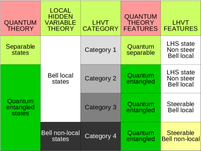
Figure 1: The Quantum Theory and the Local Hidden Variable Theory Classification Schemes (QTCS and LHVCS). The two categories of quantum states in the QTCS are shown in the left column and the two basic categories of quantum states in the LHVCS are shown in the second left column. The four more detailed categories of quantum states in the LHVCS are shown in the third left column, whilst the right two columns lists the features of the four categories of LHVCS states in both the QTCS and LHVCS schemes.

The mixed states introduced by Werner Werner89a provide examples of the three categories of Bell local states and of the Bell non-local states. These are certain $U\otimes U$ invariant states ($(\widehat{U}\otimes\widehat{U})\,\widehat{\rho}_{W}\,(\widehat{U}^{{\dagger}}\otimes\widehat{U}^{{\dagger}})=\widehat{\rho}_{W}$, where $\widehat{U}$ is any unitary operator) for two $d$ dimensional sub-systems. Depending on the parameter $\eta$ (or $\phi$) the Werner states (see Eq, (127)) may be separable or entangled. They may also be Bell local and in one of the three categories described above, or they may be Bell non-local. For completeness the Werner states are described in Appendix E. The GHZ (or maximally entangled) pure state for two sub-systems, each consisting of a spin $1/2$ particle considered by He et al. He11a , and given by $(\left|\frac{1}{2},+\frac{1}{2}\right\rangle_{A}\left|\frac{1}{2},+\frac{1}{2}\right\rangle_{B}+\left|\frac{1}{2},-\frac{1}{2}\right\rangle_{A}\left|\frac{1}{2}-\frac{1}{2}\right\rangle_{B})/\sqrt{2}$ is an example of a Category 3 state, since it is entangled and steerable, but is still Bell-local. As mentioned previously, the singlet state Clauser69a for the same system - given by $(\left|\frac{1}{2},+\frac{1}{2}\right\rangle_{A}\left|\frac{1}{2},+\frac{1}{2}\right\rangle_{B}-\left|\frac{1}{2},-\frac{1}{2}\right\rangle_{A}\left|\frac{1}{2}-\frac{1}{2}\right\rangle_{B})/\sqrt{2}$ - is an example of a Category 4 state, since it is entangled, steerable, and is Bell non-local as it violates a Bell inequality.

IV Tests for EPR Steering in Bipartite Systems

IV.1 General Considerations

In a number of papers (see the review papers Dalton16a ; Dalton16b and references therein) various tests for quantum entanglement have been formulated, recently in the particular context of bipartite systems of identical massive bosons Dalton14a . The focus was on the situation of single mode sub-systems. These include spin and two mode quadrature squeezing, Bloch vector and correlation tests. An important issue then is: Are these tests also valid for detecting EPR steering or do some of them fail? As for the entanglement tests, for the EPR steering tests we also focus on single mode sub-systems. Of course any test that detects EPR steering must of necessity also detect entanglement, but a test that demonstrates entanglement does not necessarily demonstrate EPR steering. In this situation we are looking for conditions where there is no local hidden state for sub-system $B$ - or in other words, the quantum state does not have a joint measurement probability as in Eqs. (26) and (27) for Category 1 or Category 2 states. Thus EPR steering requires the failure of the LHS model. As the tests for quantum entanglement previously obtained have already found the conditions under which Category 1 probabilities fail, we then know that the quantum state must be in Category 2, Category 3 or Category 4. If we can then show that it is not in Category 2 because the joint measurement probability (27) also fails, then the state must be in Category 3 or Category 4 - in other words it is an EPR steerable state. We would then have found a test for EPR steering. Note that for the Category 2 states the sub-system $A$ probabilities $P(\alpha|\Omega_{A},c,\lambda)$ in LHVT are not given by a quantum expression involving a sub-system density operator. This feature must be taken into account when considering the tests for EPR steering. However, the issue of how to treat mean values and variances in the context of LHVT in general requires some consideration, so we have set this out in Appendix C.

Note however that a test that demonstrates EPR steering only shows that the quantum state is either Category 3 or Category 4, both of which are entangled states. To demonstrate Bell non-locality (Category 4 states) will require different tests - notably those involving violations of a Bell inequality. This will be the subject of a later paper. As has been emphasised in Section I, showing that a Bell inequality is violated demonstrates that the state cannot be in Categories 1, 2 or 3, so it must be a Bell non-local state (Category 4). However, we emphasise again the point that the tests presented here show what category (or categories) the quantum state cannot belong to - which does not always determine what category of quantum state must apply. The tests are those of sufficiency not necessity.

In the present paper, as in previous work in Refs. Dalton14a ; Dalton16a ; Dalton16b , we focus on tests for bipartite systems involving identical massive bosons. Consequently, when quantum states either for the overall system or for a sub-system are involved these must comply with the symmetrization principle and super-selection rules involving the total boson number for either the overall system or for the sub-system. In particular, for Category 2 states (as well as Category 1 states) the local hidden state $\widehat{\rho}^{B}(c,\lambda)$ for the sub-system $B$ that is treated quantum mechanically must have zero coherences between Fock states with differing sub-system boson number $N_{B}$. The LHS must be a possible quantum state for sub-system $B$. The issue of super-selection rules is discussed fully in Dalton16a .

Also, as in these papers both the overall system and the two sub-systems will be specified in terms of modes (or single particle states that the particles may occupy) based on a second quantization treatment, rather than in terms of labeled identical particles - as might be thought appropriate in a first quantization method. Cases with differing numbers of particles are just different states of the (multi) modal system, not different systems, as in first quantization.

In addition, since the mean values of various observables are involved in the tests for showing the state is not Category 2, we can use Eqs. (LABEL:Eq.MeanValueSingleMeastQThyLHVT) and (LABEL:Eq.MeanValueJointMeastsQThyLHVT) for overall system mean values to replace LHVT theory expressions by quantum theory expressions at suitable stages in the derivations - both when a sub-system $B$ LHS $\widehat{\rho}^{B}(c,\lambda)$ occurs or when we wish to evaluate the mean value of a sub-system $A$ observable $\Omega_{A}$ allowing for all values of the hidden variables $\lambda$. However, there will be situations for Category 2 states where we need to consider the mean value of a sub-system $A$ observable $\Omega_{A}$ when the hidden variables have particular values. In this case some general properties of classical probabilities $P(\alpha|\Omega_{A},c,\lambda)$ are useful. These are not dependent on $P(\alpha|\Omega_{A},c,\lambda)$ being obtained from a hidden state density operator $\widehat{\rho}^{A}(c,\lambda)$. One is that the mean of the square of a real observable is never less than the square of the mean for the observable, that is

$$\left\langle\Omega_{A}^{2}(c,\lambda)\right\rangle\geq(\left\langle\Omega_{A}(c,\lambda)\right\rangle)^{2}.$$ (31)

Another, is a Cauchy inequality

$$\sum\limits_{\lambda}C(\lambda)\,P(\lambda|c)\geq\left(\sum\limits_{\lambda}\sqrt{C(\lambda)}\,P(\lambda|c)\right)^{2}$$ (32)

for $C(\lambda)\geq 0$, such as the case $\ C(\lambda)=\left\langle\Omega_{A}^{2}(c,\lambda)\right\rangle$. The proof of the first is elementary, the second is proved in Ref. Dalton16a . These results are only used to derive correlation tests (see Appendix I).

Finally, since LHVT deals with physical quantities that are classical observables we need to express various non-Hermitian quantum mechanical operators that we need to consider - such as mode annihilation and creation operators - in terms of quantum operators that are Hermitian. Any non-Hermitian operator $\widehat{\Omega}$ can always be expressed in terms of Hermitian operators $\widehat{\Omega}_{1}$ and $\widehat{\Omega}_{2}$ as $\widehat{\Omega}=$ $\widehat{\Omega}_{1}+i$ $\widehat{\Omega}_{2}$ and the latter operators would be equivalent to classical observables $\Omega_{1}$ and $\Omega_{2}$, so the corresponding classical observable will be $\Omega=$ $\Omega_{1}+i$ $\Omega_{2}$. The mean value $\langle\widehat{\Omega}\rangle$ will then be equal to $\langle\widehat{\Omega}_{1}\rangle+i\langle\widehat{\Omega}_{2}\rangle$. Note that two independent sets of measurements for the generally incompatible $\widehat{\Omega}_{1}$ and $\widehat{\Omega}_{2}$ would be needed to separately determine $\langle\widehat{\Omega}_{1}\rangle$ and $\langle\widehat{\Omega}_{2}\rangle$. For the corresponding classical observable we take $\langle\Omega\rangle=\langle\Omega_{1}\rangle+i\langle\Omega_{2}\rangle$ - see Eq. (115) in Appendix C. The bosonic annihilation and creation operators for each of the single mode sub-systems are not Hermitian, so we replace these by pairs of quadrature operators $\widehat{x},\widehat{p}$, which are then associated with classical quadrature observables $x,p$ when LHVT is being considered. As we will see, we also need new auxiliary Hermitian operators $\widehat{U},\widehat{V}$ as well, which are sums of products of quadrature operators and these will also be associated with classical observables $U,V$ in the LHVT. All the physical observables that we need to consider have quantum operators that can be written as linear combinations of products $\widehat{\Omega}_{A}\otimes\widehat{\Omega}_{B}$, where both $\widehat{\Omega}_{A}$ and $\widehat{\Omega}_{B}$ are Hermitian - including cases where $\widehat{\Omega}_{A}=\widehat{1}_{A}$ or $\widehat{\Omega}_{B}=\widehat{1}_{B}$. Such products can then be replaced by $\Omega_{A}\otimes\Omega_{B}$, where $\Omega_{A}$ and $\Omega_{B}$ are the corresponding classical observables. Using this procedure both quantum and hidden variable theory expressions can be used for the joint measurement probabilities and mean values.

IV.2 Spin and Quadrature Tests for EPR Steering

We now obtain a number of inequalities for spin and quadrature observables that apply for Category 2 (and Category 1) states and apply these to obtain tests for EPR steering. First, we consider whether tests that have been shown to be sufficient to demonstrate quantum entanglement (violation of Category 1) (see Ref. Dalton16b for details) are also valid for demonstrating EPR steering. Obviously a test that demonstrates EPR steering must also demonstrate quantum entanglement, but a test that demonstrates entanglement does not necessarily demonstrate EPR steering. We first consider the Bloch vector tests, then spin squeezing tests for $S_{z\text{ }}$and for the other spin components, followed by planar spin variance tests (such as the Hillery-Zubairy test) which involve the sum of the variances for $S_{x\text{ }}$and $S_{y\text{ }}$and finally two mode quadrature squeezing tests . Of these possible tests, the Bloch vector test, spin squeezing in any spin component, the Hillery-Zubairy spin variance test and squeezing in any two mode quadrature are valid for demonstrating EPR steering. We also consider a generalised version of the Hillery- Zubairy spin variance test, which also shows that EPR steering occurs. Finally, we consider for completeness weak and strong correlation tests in Appendix I, though these are equivalent to certain of the tests involving spin operators already set out in this Section.

IV.3 Quadrature Amplitudes

The non-Hermitian quantum mode annihilation or creation operators can be replaced by their Hermitian components,which are the quadrature operators. In quantum theory these are given by

$$\widehat{x}_{A} =\frac{1}{\sqrt{2}}(\widehat{a}+\widehat{a}^{{\dagger}}), \widehat{p}_{A} =\frac{1}{\sqrt{2}i}(\widehat{a}-\widehat{a}^{{\dagger}}),$$

$$\widehat{x}_{B} =\frac{1}{\sqrt{2}}(\widehat{b}+\widehat{b}^{{\dagger}}), \widehat{p}_{B} =\frac{1}{\sqrt{2}i}(\widehat{b}-\widehat{b}^{{\dagger}}),$$ (33)

which have the same commutation rules as the position and momentum operators for distinguishable particles in units where $\hbar=1$. Thus $[\widehat{x}_{A},\widehat{p}_{A}]=[\widehat{x}_{B},\widehat{p}_{B}]=i$ as for cases where $A$, $B$ were distinguishable particles. It is then reasonable to assume that there are equivalent classical observables $x_{A},p_{A},x_{B},p_{B}$ and that their measurement outcomes would be real numbers, and further more for sub-systems not being treated quantum mechanically (such as sub-system $A$ in the context of Category 2 states) these outcomes can actually be measured in experiment and probabilities and mean values such as $P(\alpha|\Omega_{A},c,\lambda)$ and $\left\langle\Omega_{A}(\lambda)\right\rangle$ can be assigned as in a hidden variable treatment of sub-system $A$. However, in considering Category 2 states the probabilities and mean values such as $P(\beta|\Omega_{B},c,\lambda)$ and $\left\langle\Omega_{B}(\lambda)\right\rangle$ for the sub-system $B$ are also given by quantum expressions involving sub-system density operators $\widehat{\rho}^{B}(\lambda)$.

We can write the mode annihilation and creation operators in terms of the quadrature operators as $\widehat{a}=(\widehat{x}_{A}+i\widehat{p}_{A})/\sqrt{2}$, $\widehat{a}^{{\dagger}}=(\widehat{x}_{A}-i\widehat{p}_{A})/\sqrt{2}$, $\widehat{b}=(\widehat{x}_{B}+i\widehat{p}_{B})/\sqrt{2}$, $\widehat{b}^{{\dagger}}=(\widehat{x}_{B}-i\widehat{p}_{B})/\sqrt{2}$ and then show that important observables can be expressed in terms of the quadrature operators. In the case of the spin operators (defined as $\widehat{S}_{x}=(\widehat{b}^{{\dagger}}\widehat{a}+\widehat{a}^{{\dagger}}\widehat{b})/2$, $\widehat{S}_{y}=(\widehat{b}^{{\dagger}}\widehat{a}-\widehat{a}^{{\dagger}}\widehat{b})/2i$, $\widehat{S}_{z}=(\widehat{b}^{{\dagger}}\widehat{b}-\widehat{a}^{{\dagger}}\widehat{a})/2$) and the number operators (defined as $\widehat{N}=$ $\widehat{N}_{A}+\widehat{N}_{B}$ with $\widehat{N}_{A}=\widehat{a}^{{\dagger}}\widehat{a}$, $\widehat{N}_{B}=\widehat{b}^{{\dagger}}\widehat{b}$ being the separate mode number operators - note that $\widehat{S}_{x}^{2}+\widehat{S}_{y}^{2}+\widehat{S}_{z}^{2}=\frac{\widehat{N}}{2}(\frac{\widehat{N}}{2}+1)$), all these quantities can be expressed in terms of the quadrature operators as follows

$$\widehat{S}_{x} = \frac{1}{2}(\widehat{x}_{A}\widehat{x}_{B}+\widehat{p}_{A}\widehat{p}_{B}),\qquad\widehat{S}_{y}=\frac{1}{2}(\widehat{p}_{A}\widehat{x}_{B}-\widehat{x}_{A}\widehat{p}_{B}),$$

$$\widehat{S}_{z} = \frac{1}{4}(\widehat{x}_{B}^{2}-\widehat{x}_{A}^{2}+\widehat{p}_{B}^{2}-\widehat{p}_{A}^{2})-\frac{1}{2}\widehat{V}_{B}+\frac{1}{2}\widehat{V}_{A},$$

$$\widehat{N} = \frac{1}{2}(\widehat{x}_{B}^{2}+\widehat{x}_{A}^{2}+\widehat{p}_{B}^{2}+\widehat{p}_{A}^{2})-\widehat{V}_{B}-\widehat{V}_{A},$$

which are all linear combinations of products of two quadrature operators. Here we have introduced the auxiliary Hermitian operators

$$\widehat{V}_{A} = \frac{1}{2i}(\widehat{x}_{A}\widehat{p}_{A}-\widehat{p}_{A}\widehat{x}_{A})=\frac{1}{2}\widehat{1}_{A\text{ }},$$

$$\widehat{V}_{B} = \frac{1}{2i}(\widehat{x}_{B}\widehat{p}_{B}-\widehat{p}_{B}\widehat{x}_{B})=\frac{1}{2}\widehat{1}_{B\text{ }},$$ (35)

using the commutation rules. These operators could represent observables in quantum theory, albeit rather useless ones since all eigenstates have the same eigenvalue of $1/2$. In terms of the quadrature and auxiliary operators the mode number and mode number difference operators are:

$$\widehat{N}_{A} = \frac{1}{2}(\widehat{x}_{A}^{2}+\widehat{p}_{A}^{2})-\widehat{V}_{A},$$

$$\widehat{N}_{B} = \frac{1}{2}(\widehat{x}_{B}^{2}+\widehat{p}_{B}^{2})-\widehat{V}_{B},$$ (36)

$$\widehat{N}_{-} = \widehat{N}_{B}-\widehat{N}_{A}=2\widehat{S}_{z},$$ (37)

$$= \frac{1}{2}(\widehat{x}_{B}^{2}+\widehat{p}_{B}^{2}-\widehat{x}_{A}^{2}-\widehat{p}_{A}^{2})-\widehat{V}_{B}+\widehat{V}_{A}.$$

As spin squeezing was a test for entanglement Dalton16b , spin squeezing expressions for $\widehat{S}_{x}^{2}$, $\widehat{S}_{y}^{2}$ and $\widehat{S}_{z}^{2}$ will be required. We find that for $\widehat{S}_{x}^{2}$ and $\widehat{S}_{y}^{2}$

$$\widehat{S}_{x}^{2} = \frac{1}{4}(\widehat{x}_{A}^{2}\widehat{x}_{B}^{2}+\widehat{p}_{A}^{2}\widehat{p}_{B}^{2})+\frac{1}{2}(\widehat{U}_{A}\widehat{U}_{B}-\widehat{V}_{A}\widehat{V}_{B}),$$ (38)

$$\widehat{S}_{y}^{2} = \frac{1}{4}(\widehat{p}_{A}^{2}\widehat{x}_{B}^{2}+\widehat{x}_{A}^{2}\widehat{p}_{B}^{2})-\frac{1}{2}(\widehat{U}_{A}\widehat{U}_{B}+\widehat{V}_{A}\widehat{V}_{B}).$$ (39)

The spin operators thus involve the quadrature operators for both modes. Here we have introduced two further distinct auxiliary Hermitian combinations of the quadrature operators for each mode:

$$\widehat{U}_{A} = \frac{1}{2}(\widehat{x}_{A}\widehat{p}_{A}+\widehat{p}_{A}\widehat{x}_{A})=\frac{1}{2i}((\widehat{a})^{2}-(\widehat{a}^{{\dagger}})^{2}),$$

$$\widehat{U}_{B} = \frac{1}{2}(\widehat{x}_{B}\widehat{p}_{B}+\widehat{p}_{B}\widehat{x}_{B})=\frac{1}{2i}((\widehat{b})^{2}-(\widehat{b}^{{\dagger}})^{2}),$$ (40)

where using the commutation rules the operators $\widehat{U}_{A}$ and $\widehat{U}_{B}$ can also be expressed in terms of mode annihilation and creation operators.

In addition to the spin operators we can also define two mode quadrature operators in terms of the quadrature operators for both modes Dalton16b . These depend on a phase parameter $\theta$. There are two sets given by

$$\widehat{X}_{\theta}(\pm) =\frac{1}{2}\left(\widehat{a}\,e^{-i\theta}\pm\widehat{b}\,e^{+i\theta}+\widehat{a}^{{\dagger}}\,e^{+i\theta}\pm\widehat{b}^{{\dagger}}\,e^{-i\theta}\right),$$

$$\widehat{P}_{\theta}(\pm) =\frac{1}{2i}\left(\widehat{a}\,e^{-i\theta}\mp\widehat{b}\,e^{+i\theta}-\widehat{a}^{{\dagger}}\,e^{+i\theta}\pm\widehat{b}^{{\dagger}}\,e^{-i\theta}\right).$$ (41)

It is easy to see that $\widehat{P}_{\theta}(\pm)=\widehat{X}_{\theta+\pi/2}(\pm)$ and that $[\widehat{X}_{\theta}(+),\widehat{P}_{\theta}(+)]=[\widehat{X}_{\theta}(-),\widehat{P}_{\theta}(-)]=i$. The Heisenberg uncertainty principle is given by $\left\langle\Delta X_{\theta}^{2}(\pm)\right\rangle\left\langle\Delta P_{\theta}^{2}(\pm)\right\rangle\geq 1/4$ and a state is two mode quadrature squeezed if one of $\left\langle\Delta X_{\theta}^{2}(\pm)\right\rangle$ or $\left\langle\Delta P_{\theta}^{2}(\pm)\right\rangle$ is less than $1/2$. In Reference Dalton16b we showed that two mode quadrature squeezing was a sufficiency test for entanglement. We can write the two mode quadrature operators in terms of the single mode quadrature operators as:

$$\widehat{X}_{\theta}(\pm) = \frac{1}{\sqrt{2}}\left(\widehat{x}_{A}\cos\theta+\widehat{p}_{A}\sin\theta\pm\widehat{x}_{B}\cos\theta\pm\widehat{p}_{B}\sin\theta\right),$$

$$\widehat{P}_{\theta}(\pm) = \frac{1}{\sqrt{2}}\left(-\widehat{x}_{A}\sin\theta+\widehat{p}_{A}\cos\theta\mp\widehat{x}_{B}\sin\theta\pm\widehat{p}_{B}\cos\theta\right).$$

The square of the two mode quadrature operators $\widehat{X}_{\theta}(\pm)$ are given by

$$\widehat{X}_{\theta}(\pm)^{2} = \frac{1}{2}\left\{\widehat{x}_{A}^{2}\cos^{2}\theta+\widehat{p}_{A}^{2}\sin^{2}\theta+2\widehat{U}_{A}\sin\theta\cos\theta\right\}$$

$$+\frac{1}{2}\left\{\widehat{x}_{B}^{2}\cos^{2}\theta+\widehat{p}_{B}^{2}\sin^{2}\theta+2\widehat{U}_{B}\sin\theta\cos\theta\right\}$$

$$\pm\left\{\widehat{x}_{A}\widehat{x}_{B}\cos^{2}\theta+\widehat{p}_{A}\widehat{p}_{B}\sin^{2}\theta\right.$$

$$\left.\qquad+\widehat{x}_{A}\widehat{p}_{B}\sin\theta\cos\theta+\widehat{p}_{A}\widehat{x}_{B}\sin\theta\cos\theta\right\}.$$

The expression for $\widehat{P}_{\theta}(\pm)^{2}$ can be obtained using $\widehat{P}_{\theta}(\pm)=\widehat{X}_{\theta+\pi/2}(\pm)$.

The fundamental quantum Hermitian operators $\widehat{x}_{A}$, $\widehat{p}_{A}$, $\widehat{x}_{B}$, $\widehat{p}_{B}$ for the two mode system plus the auxiliary Hermitian operators $\widehat{U}_{A}$, $\widehat{V}_{A}$, $\widehat{U}_{B}$, $\widehat{V}_{B}$ all correspond to physical quantities that could be measured, with real eigenvalues as the outcomes. Following the general approach described in Section I, for local hidden variable theory these quantities correspond to classical observables $x_{A}$, $p_{A}$, $x_{B}$, $p_{B}$ and $U_{A},V_{A},U_{B},V_{B}$, for which single observable hidden variable probabilities $P(\alpha|\Omega_{A},c,\lambda)$ and $P(\beta|\Omega_{B},c,\lambda)$ apply - from which joint probabilities $P(\alpha,\beta|\Omega_{A},\Omega_{B},c)$ can be obtained via (9). The physical observables involved in the tests such as the spin operators, their squares and the number operators can all be expressed in terms of the quadrature and auxiliary operators as sums of products of the form $\widehat{\Omega}_{A}\otimes\widehat{\Omega}_{B}$. For the local hidden variable theory treatment the corresponding classical observables will be the same as the quantum expressions, but now with the quantum Hermitian operators replaced by the corresponding classical observable. For the classical spin components $S_{x}$, $S_{y}$ and $S_{z}$ and the number observable $N$ the expressions in terms of quadrature amplitudes $x$, $p$ and auxiliary observables $U$, $V$ are

$$S_{x} = \frac{1}{2}(x_{A}x_{B}+p_{A}p_{B}),\qquad S_{y}=\frac{1}{2}(p_{A}x_{B}-x_{A}p_{B}),$$

$$S_{z} = \frac{1}{4}(x_{B}^{2}-x_{A}^{2}+p_{B}^{2}-p_{A}^{2})-\frac{1}{2}V_{B}+\frac{1}{2}V_{A},$$

$$N = \frac{1}{2}(x_{B}^{2}+x_{A}^{2}+p_{B}^{2}+p_{A}^{2})-V_{B}-V_{A}\,.$$

The expressions in terms of quadrature amplitudes $x$, $p$ and auxiliary observables $U$, $V$ for the sub-system particle numbers and their difference are

$$N_{A} = \frac{1}{2}(x_{A}^{2}+p_{A}^{2})-V_{A},\qquad N_{B}=\frac{1}{2}(x_{B}^{2}+p_{B}^{2})-V_{B},$$

$$N = N_{A}+N_{B},$$

$$N_{-} = N_{B}-N_{A}=2S_{z},$$ (45)

$$= \frac{1}{2}(x_{B}^{2}+p_{B}^{2}-x_{A}^{2}-p_{A}^{2})-V_{B}+V_{A}\,.$$

The two mode quadrature observables are given by

$$X_{\theta}(\pm) =\frac{1}{\sqrt{2}}\left(x_{A}\cos\theta+p_{A}\sin\theta\pm x_{B}\cos\theta\pm p_{B}\sin\theta\right),$$

$$P_{\theta}(\pm) =\frac{1}{\sqrt{2}}\left(-x_{A}\sin\theta+p_{A}\cos\theta\mp x_{B}\sin\theta\pm p_{B}\cos\theta\right).$$

(46)

For completeness we set out expressions for other observables in Appendix D. The reverse process for the replacement of the classical observables $x_{A}$, $x_{B}$, $p_{A}$, $p_{B}$ by $\widehat{x}_{A}$, $\widehat{x}_{B}$, $\widehat{p}_{A}$, $\widehat{p}_{B}$ and $U_{A}$, $U_{B}$, $V_{A}$, $V_{B}$ by $\widehat{U}_{A}$, $\widehat{U}_{B}$, $\widehat{V}_{A}$, $\widehat{V}_{B}$ requires using (33), (40) and (35) to give the correct quantum Hermitian operators. This requires writing $V_{A}=(x_{A}p_{A}-p_{A}x_{A})/2i$ and $U_{A}=(x_{A}p_{A}+p_{A}x_{A})/2$ etc. before substituting $x_{A}$ by $\widehat{x}_{A}$, $p_{A}$ by $\widehat{p}_{A}$ etc., rather than $V_{A}=0$ and $U_{A}=2x_{A}p_{A}$ etc., but this is not surprising as c-number variables are not mathematically identical to Hermitian operators. Carrying out this replacement in the classical spin components $S_{x}$, $S_{y}$ and $S_{z}$ and the number observable $N$ also gives the correct quantum operators, as also occurs for the squares of these observables as well. Once again we emphasise that we only need single measurement LHVT probabilities $P(\alpha|\Omega_{A},c,\lambda)$ with $\Omega_{A}=x_{A}$, $p_{A}$, $U_{A}$ or $V_{A}$ and $P(\beta|\Omega_{B},c,\lambda)$ with $\Omega_{B}=x_{B}$, $p_{B}$, $U_{B}$ or $V_{B}$ to treat the classical observables such as $S_{x}$, $S_{y}$ and $S_{z}$ and $N$ or $X_{\theta}(\pm)$, $P_{\theta}(\pm)$ via hidden variable theory.

The local hidden variable theory for these new observables is defined by measurement probability functions for each sub-system. For sub-system $A$ this will be $P(\alpha_{A},\beta_{A},\xi_{A},\eta_{A}|x_{A},p_{A},U_{A},V_{A},c,\lambda)$ for the measurement outcomes $\alpha_{A},\beta_{A},\xi_{A},\eta_{A}$ for $x_{A}$, $p_{A}$, $U_{A}$ and $V_{A}$ respectively, with an analogous probability for $x_{B}$, $p_{B}$, $U_{B}$ and $V_{B}$. Note that as the measurement outcomes for $V_{A}$ and $V_{B}$ are required to be the same as in quantum theory for any choice of preparation probability $P(\lambda|c)$, we must have

$$P(\alpha_{A},\beta_{A},\xi_{A},\eta_{A}|x_{A},p_{A},U_{A},V_{A},c,\lambda)\\ =\delta_{\eta_{A},1/2}Q(\alpha_{A},\beta_{A},\xi_{A}|x_{A},p_{A},U_{A},c,\lambda),\\ P(\alpha_{B},\beta_{B},\xi_{B},\eta_{B}|x_{B},p_{B},U_{B},V_{B},c,\lambda)\\ =\delta_{\eta_{B},1/2}Q(\alpha_{B},\beta_{B},\xi_{B}|x_{B},p_{B},U_{B},c,\lambda).$$ (47)

These requirements have implications for the mean values $\left\langle V_{A}(\lambda)\right\rangle$, though only the final mean value $\left\langle V_{A}\right\rangle$ is required for the EPR steering tests.

IV.4 Bloch Vector Test for EPR Steering

IV.4.1 Mean Values of Spin Components S_xand S_y - Category 2 States 

We now consider the mean value for spin components for the Category 2 states. For example, in the case of the spin component $S_{x}$

$$\left\langle S_{x}\right\rangle =\sum\limits_{\lambda}P(\lambda|c)\left\langle S_{x}(\lambda)\right\rangle$$

$$=\frac{1}{2}\sum\limits_{\lambda}\bigl{(}\left\langle x_{A}(\lambda)\right\rangle\left\langle x_{B}(\lambda)\right\rangle_{Q}+\left\langle p_{A}(\lambda)\right\rangle\left\langle p_{B}(\lambda)\right\rangle_{Q}\bigr{)}$$

$$\qquad\qquad\times P(\lambda|c)$$ (48)

using (LABEL:Eq.SpinCompts) and (12). This expression involves the hidden variable mean values for the (classical) observables $x_{A}$ and $p_{A}$ of sub-system $A$ and the local hidden state mean values for the quantum quadrature operators $\widehat{x}_{B}$ and $\widehat{p}_{B}$. The latter must also correspond to quantum mean values, for a physically realisable quantum state for sub-system $B$. Thus $\left\langle x_{B}(\lambda)\right\rangle_{Q}=\text{Tr}(\widehat{x}_{B}\widehat{\rho}^{B}(\lambda))$ and $\left\langle p_{B}(\lambda)\right\rangle_{Q}=\text{Tr}(\widehat{p}_{B}\widehat{\rho}^{B}(\lambda))$. Since sub-system $B$ is to be treated quantum mechanically then the density operator $\widehat{\rho}^{B}(\lambda)$ would be required to both satisfy the symmetrisation principle and be local particle number SSR compliant. Hence there is a constraint based on the local hidden state $\widehat{\rho}^{B}(\lambda)$ being a possible state for sub-system $B$ that requires the state to be local particle number SSR compliant.

In this case then since both $\widehat{x}_{B}$ and $\widehat{p}_{B}$ are just linear combinations of $\widehat{b}$ and $\widehat{b}^{{\dagger}}$ we have

$$\left\langle x_{B}(\lambda)\right\rangle_{Q} = \text{Tr}\frac{1}{\sqrt{2}}(\widehat{b}+\widehat{b}^{{\dagger}})\widehat{\rho}^{B}(\lambda)=0,$$

$$\left\langle p_{B}(\lambda)\right\rangle_{Q} = \text{Tr}\frac{1}{\sqrt{2}i}(\widehat{b}-\widehat{b}^{{\dagger}})\widehat{\rho}^{B}(\lambda)=0,$$ (49)

$$\left\langle S_{x}(\lambda)\right\rangle = 0,\qquad\left\langle S_{y}(\lambda)\right\rangle=0,$$ (50)

and thus for Category 2 states

$$\left\langle S_{x}\right\rangle=0,\qquad\left\langle S_{y}\right\rangle=0\,.$$ (51)

We do not need to know the outcome for $\left\langle x_{A}(\lambda)\right\rangle$ or $\left\langle p_{A}(\lambda)\right\rangle$.

So that if LHVT is to give the same prediction as quantum theory then on reverting to quantum operators and using (LABEL:Eq.MeanValueJointMeastsQThyLHVT) we have for Category 2 states

$$\left\langle\widehat{S}_{x}\right\rangle=0,\qquad\text{and}\qquad\left\langle\widehat{S}_{y}\right\rangle=0.$$ (52)

These two results are the same as for a quantum separable (Category 1) state.

IV.4.2 Bloch Vector Test

From (52) for Category 2 (or Category 1) states we immediately see that if

$$\left\langle\widehat{S}_{x}\right\rangle\neq 0\qquad\text{or}\qquad\left\langle\widehat{S}_{y}\right\rangle\neq 0,$$ (53)

then the quantum state cannot be in Category 2 (or Category 1). The Bloch vector test $\langle\widehat{S}_{x}\rangle\neq 0$ or $\langle\widehat{S}_{y}\rangle\neq 0$ now also shows that the state is EPR steered as well as just being entangled.

Experiments in two mode BEC by Gross10a ; Egorov11a have found non-zero behaviour for $\langle\widehat{S}_{x}\rangle$, $\langle\widehat{S}_{y}\rangle$. These experiments therefore demonstrate EPR steering, though only entanglement was claimed to have been shown Gross10a . The application of the Bloch vector test for EPR steering to the experiment in Egorov11a is discussed more fully elsewhere Opanchuk17a .

IV.5 Spin Squeezing Tests for EPR Steering

IV.5.1 Mean Values of Spin Component S_zand Number N - Category 2 States 

For the other spin component $S_{z}$ we find using (45) that for the Category 2 states

$$\left\langle S_{z}\right\rangle=\frac{1}{2}\left\langle 1_{A}\otimes N_{B}\right\rangle-\frac{1}{2}\left\langle N_{A}\otimes 1_{B}\right\rangle.$$ (54)

As in the quantum separable state case $\left\langle S_{z}\right\rangle$ is not necessarily zero.

IV.5.2 Variances of Spin Components S_xand S_y - Category 2 States

As $\langle S_{x}(\lambda)\rangle=\langle S_{y}(\lambda)\rangle=0$ from (50) we see that $\langle\Delta S_{x}^{2}(\lambda)\rangle=\langle S_{x}^{2}(\lambda)\rangle$ and $\langle\Delta S_{y}^{2}(\lambda)\rangle=\langle S_{y}^{2}(\lambda)\rangle$. Using (LABEL:Eq.MeanValueJointMeastsQThyLHVT), the LHVT expression for $S_{x}^{2}$ obtained from the classical form of (38) and after applying the inequality (114) we then have the following inequalities for Category 2 states

$$\left\langle\Delta S_{x}^{2}\right\rangle\geq \sum\limits_{\lambda}P(\lambda|c)$$

$$\times\left[\frac{1}{4}(\left\langle x_{A}^{2}(\lambda)\right\rangle\left\langle x_{B}^{2}(\lambda)\right\rangle_{Q}+\left\langle p_{A}^{2}(\lambda)\right\rangle\left\langle p_{B}^{2}(\lambda)\right\rangle_{Q})\right.$$

$$\left.\quad+\frac{1}{2}(\left\langle U_{A}(\lambda)\right\rangle\left\langle U_{B}(\lambda)\right\rangle_{Q}-\left\langle V_{A}(\lambda)\right\rangle\left\langle V_{B}(\lambda)\right\rangle_{Q})\right]$$

$$\left\langle\Delta S_{y}^{2}\right\rangle\geq \sum\limits_{\lambda}P(\lambda|c)$$

$$\times\left[\frac{1}{4}(\left\langle p_{A}^{2}(\lambda)\right\rangle\left\langle x_{B}^{2}(\lambda)\right\rangle_{Q}+\left\langle x_{A}^{2}(\lambda)\right\rangle\left\langle p_{B}^{2}(\lambda)\right\rangle_{Q})\right.$$

$$\left.\quad-\frac{1}{2}(\left\langle U_{A}(\lambda)\right\rangle\left\langle U_{B}(\lambda)\right\rangle_{Q}+\left\langle V_{A}(\lambda)\right\rangle\left\langle V_{B}(\lambda)\right\rangle_{Q})\right].$$

IV.5.3 Evaluation of Expressions Needed - Category 2 States

To consider spin squeezing, spin variance and correlation tests for EPR steering based on the Category 2 states we will need to consider the following additional quantum theory based expressions: $\left\langle x_{B}^{2}(\lambda)\right\rangle_{Q}$, $\left\langle p_{B}^{2}(\lambda)\right\rangle_{Q}$, $\left\langle V_{B}(\lambda)\right\rangle_{Q}$, $\left\langle U_{B}(\lambda)\right\rangle_{Q}$ and the following non-quantum expressions $\left\langle x_{A}^{2}(\lambda)\right\rangle$, $\left\langle p_{A}^{2}(\lambda)\right\rangle$, $\left\langle V_{A}(\lambda)\right\rangle$.

Starting with the quantum theory expressions (33) we find that

$$\left\langle x_{B}^{2}(\lambda)\right\rangle_{Q} = \text{Tr}((\widehat{b}^{{\dagger}}\widehat{b})\widehat{\rho}^{B}(\lambda))+\frac{1}{2},$$ (56)

$$= \left\langle N_{B}(\lambda)\right\rangle_{Q}+\frac{1}{2},$$

$$\left\langle p_{B}^{2}(\lambda)\right\rangle_{Q} = \left\langle N_{B}(\lambda)\right\rangle_{Q}+\frac{1}{2},$$ (57)

where the commutation rules have been used and the SSR constraints eliminate the $\text{Tr}((\widehat{b})^{2}\widehat{\rho}^{B}(\lambda))$ and $\text{Tr}((\widehat{b}^{{\dagger}})^{2}\widehat{\rho}^{B}(\lambda))$ terms. Note that $\left\langle N_{B}(\lambda)\right\rangle_{Q}\geq 0$.

Then using (40) we find that

$$\left\langle U_{B}(\lambda)\right\rangle_{Q} = \frac{1}{2i}\text{Tr}((\widehat{b})^{2}-(\widehat{b}^{{\dagger}})^{2})\widehat{\rho}^{B}(\lambda)$$ (58)

$$= 0,$$

again due to the SSR constraints on the hidden state $\widehat{\rho}^{B}(\lambda)$.

Also, using (35)

$$\left\langle V_{B}(\lambda)\right\rangle_{Q} = \frac{1}{2}\text{Tr}_{B}(\widehat{1}_{B}\widehat{\rho}^{B}(\lambda))$$ (59)

$$= \frac{1}{2}$$

since the trace of a density operator is unity. Using (56), (57) and (59) we confirm the result that $\left\langle N_{B}(\lambda)\right\rangle_{Q}=\frac{1}{2}\left\langle x_{B}^{2}(\lambda)\right\rangle_{Q}+\frac{1}{2}\left\langle p_{B}^{2}(\lambda)\right\rangle_{Q}-\left\langle V_{B}(\lambda)\right\rangle_{Q}$ consistent with (45). Result (59) also follows directly from (47).

For the local hidden variable theory expressions involving sub-system $A$ we have using (45)

$$\left\langle x_{A}^{2}(\lambda)\right\rangle+\left\langle p_{A}^{2}(\lambda)\right\rangle=2\left\langle N_{A}(\lambda)\right\rangle+2\left\langle V_{A}(\lambda)\right\rangle\,.$$ (60)

Note the analogous result for sub-system $B$.

Using the results (35), (LABEL:Eq.VarSxSyIneqLHSModel)–(60) we now have for Category 2 states

$$\begin{split}&\left\langle\Delta S_{x}^{2}\right\rangle\\ &\geq\sum\limits_{\lambda}P(\lambda|c)\left(\frac{1}{2}\left(\left\langle N_{B}(\lambda)\right\rangle_{Q}+\frac{1}{2}\right)(\left\langle N_{A}(\lambda)\right\rangle+\left\langle V_{A}(\lambda)\right\rangle)\right.\\ &\left.\qquad\qquad\qquad-\frac{1}{4}\left\langle V_{A}(\lambda)\right\rangle\right)\,,\\ &\geq\frac{1}{2}\left\langle N_{A}\otimes N_{B}\right\rangle+\frac{1}{2}\left\langle V_{A}\otimes N_{B}\right\rangle+\frac{1}{4}\left\langle N_{A}\otimes 1_{B}\right\rangle\\ &\quad+\frac{1}{4}\left\langle V_{A}\otimes 1_{B}\right\rangle-\frac{1}{4}\left\langle V_{A}\otimes 1_{B}\right\rangle\,,\\ &\geq\frac{1}{2}\left\langle\widehat{N}_{A}\otimes\widehat{N}_{B}\right\rangle+\frac{1}{2}\left\langle\widehat{V}_{A}\otimes\widehat{N}_{B}\right\rangle+\frac{1}{4}\left\langle\widehat{N}_{A}\otimes\widehat{1}_{B}\right\rangle\,,\\ &\geq\frac{1}{2}\left\langle\widehat{N}_{A}\otimes\widehat{N}_{B}\right\rangle+\frac{1}{4}\left\langle\widehat{1}_{A}\otimes\widehat{N}_{B}\right\rangle+\frac{1}{4}\left\langle\widehat{N}_{A}\otimes\widehat{1}_{B}\right\rangle\,,\\ &\\ &\left\langle\Delta S_{y}^{2}\right\rangle\\ &\geq\frac{1}{2}\left\langle\widehat{N}_{A}\otimes\widehat{N}_{B}\right\rangle+\frac{1}{4}\left\langle\widehat{1}_{A}\otimes\widehat{N}_{B}\right\rangle+\frac{1}{4}\left\langle\widehat{N}_{A}\otimes\widehat{1}_{B}\right\rangle\,.\end{split}$$ (61)

Note that moving from line one to line two only involves LHVT expressions, whereas moving from line two to line three involves replacing the LHVT overall mean values by the equivalent quantum expressions, and in the next line the quantum operator $\widehat{V}_{A}$ is replaced by $\widehat{1}_{A}/2$. These inequalities are the same as those for Category 1 states (see Dalton16b ). Note that the SSR for the LHS have been used in deriving these last results. Also from (54)

$$\frac{1}{2}|\left\langle S_{z}\right\rangle|\;\leq\frac{1}{4}\left\langle 1_{A}\otimes N_{B}\right\rangle+\frac{1}{4}\left\langle N_{A}\otimes 1_{B}\right\rangle.$$ (62)

The last line follows from the LHVT expression $\langle 1_{A}\otimes N_{B}\rangle$ giving the mean number of bosons in mode $B$ and for this to be the same as the quantum theory expression $\langle\widehat{1}_{A}\otimes\widehat{N}_{B}\rangle$. As the eigenvalues of the number operator $\widehat{N}_{B}=\widehat{b}^{{\dagger}}\widehat{b}$ are never negative $\langle\widehat{1}_{A}\otimes\widehat{N}_{B}\rangle$ and hence $\langle 1_{A}\otimes N_{B}\rangle$ is never negative, so $|\langle 1_{A}\otimes N_{B}\rangle|=\langle 1_{A}\otimes N_{B}\rangle$. Similarly, $\langle N_{A}\otimes 1_{B}\rangle$ is never negative. This result is the same as that for Category 1 states (see Ref. Dalton16b ).

Combining (61) and (62) we find using LHVT that for Category 2 states

$$\left\langle\Delta S_{x}^{2}\right\rangle-\frac{1}{2}|\left\langle S_{z}\right\rangle| ~{}\geq~{} \frac{1}{2}\left\langle N_{A}\otimes N_{B}\right\rangle,$$

$$\left\langle\Delta S_{y}^{2}\right\rangle-\frac{1}{2}|\left\langle S_{z}\right\rangle| \geq \frac{1}{2}\left\langle N_{A}\otimes N_{B}\right\rangle,$$ (63)

so as the LHVT is required to predict the same results as for quantum theory we have for Category 2 states

$$\left\langle\Delta\widehat{S}_{x}^{2}\right\rangle-\frac{1}{2}\left|\left\langle\widehat{S}_{z}\right\rangle\right| ~{}\geq~{} \frac{1}{2}\left\langle\widehat{N}_{A}\otimes\widehat{N}_{B}\right\rangle\geq 0,$$ (64)

$$\left\langle\Delta\widehat{S}_{y}^{2}\right\rangle-\frac{1}{2}\left|\left\langle\widehat{S}_{z}\right\rangle\right| \geq \frac{1}{2}\left\langle\widehat{N}_{A}\otimes\widehat{N}_{B}\right\rangle\geq 0.$$ (65)

The expression $\frac{1}{2}\langle\widehat{N}_{A}\otimes\widehat{N}_{B}\rangle$ is never negative because the eigenvalues of $\widehat{N}_{A}$ and $\widehat{N}_{B}$ are never negative.

IV.5.4 Spin Squeezing Tests

From Eq. (52) we immediately see that for a quantum state where the observable $\widehat{S}_{z}$ is squeezed with respect to $\widehat{S}_{x}$ or with respect to $\widehat{S}_{y}$, then it cannot be a Category 2 state, because spin squeezing in $\widehat{S}_{z}$ requires $\langle\Delta\widehat{S}_{z}^{2}\rangle$ to be less than either $|\langle\widehat{S}_{x}\rangle|/2$ or $|\langle\widehat{S}_{y}\rangle|/2$ and this is impossible for both Category 1 (see Ref. Dalton16b ) and Category 2 states - where $\langle\widehat{S}_{x}\rangle=\langle\widehat{S}_{y}\rangle=0$. This condition also rules out $\widehat{S}_{x}$ or $\widehat{S}_{y}$ being squeezed with respect to $\widehat{S}_{z}$, or $\widehat{S}_{z}$ being squeezed with respect to $\widehat{S}_{x}$ or $\widehat{S}_{y}$. In Ref. Dalton16b it was shown that spin squeezing involving $\widehat{S}_{z}$ provided a test for entanglement. Here we see that spin squeezing involving the observable $\widehat{S}_{z}$ shows the state is EPR steered as well as merely being entangled.

From Eqs. (64) and (65) we see that for Category 2 states$\ (\langle\Delta\widehat{S}_{x}^{2}\rangle-\frac{1}{2}|\langle\widehat{S}_{z}\rangle|)\geq 0$ and $(\langle\Delta\widehat{S}_{y}^{2}\rangle-\frac{1}{2}|\langle\widehat{S}_{z}\rangle|)\geq 0$. Hence we find that for Category 2 states there is no spin squeezing in $\widehat{S}_{x}$ compared to $\widehat{S}_{y}$ (or vice versa). For Category 1 states we also find that $(\langle\Delta\widehat{S}_{x}^{2}\rangle-\frac{1}{2}|\langle\widehat{S}_{z}\rangle|)\geq\frac{1}{2}\langle\widehat{N}_{A}\otimes\widehat{N}_{B}\rangle\geq 0$ and $(\langle\Delta\widehat{S}_{y}^{2}\rangle-\frac{1}{2}|\langle\widehat{S}_{z}\rangle|)\geq\frac{1}{2}\langle\widehat{N}_{A}\otimes\widehat{N}_{B}\rangle\geq 0$ (see Eq. (31) in Ref. Dalton16b ). Hence spin squeezing in $\widehat{S}_{x}$ versus $\widehat{S}_{y}$ (or vice versa) is a test for entanglement, so the state is not in Category 1. Thus spin squeezing in $\widehat{S}_{x}$ versus $\widehat{S}_{y}$ (or vice versa) is therefore also a test for EPR steering.

Overall then we now see that spin squeezing in any spin component $\widehat{S}_{\alpha}$ with respect to another component $\widehat{S}_{\beta}$

$$\left\langle\Delta\widehat{S}_{\alpha}^{2}\right\rangle<\frac{1}{2}\left|\left\langle\widehat{S}_{\gamma}\right\rangle\right|\qquad\text{and}\qquad\left\langle\Delta\widehat{S}_{\beta}^{2}\right\rangle>\frac{1}{2}\left|\left\langle\widehat{S}_{\gamma}\right\rangle\right|$$ (66)

(where $\alpha,\beta,\gamma$ are $x,y,z$ in cyclic order) is a sufficiency test for EPR steering. Hence spin squeezing in any spin component $\widehat{S}_{\alpha}$ with respect to another component $\widehat{S}_{\beta}$ shows that the state is EPR steered as well as just being entangled.

Experiments in two mode BEC by Gross10a ; Riedel10a ; Maussang10a have found spin squeezing in $S_{z}$. These experiments therefore demonstrate EPR steering, though only entanglement was claimed to have been shown in Gross10a ; Riedel10a .

IV.6 Planar Spin Variance Tests for EPR Steering

IV.6.1 Mean Values of Total Boson Number N - Category 2 States 

For the number observable $N$ we have from (45)

$$\left\langle N\right\rangle=\left\langle 1_{A}\otimes N_{B}\right\rangle+\left\langle N_{A}\otimes 1_{B}\right\rangle.$$ (67)

This result is the same as that for Category 1 states (see Ref. Dalton16b ).

IV.6.2 Hillary-Zubairy Planar Spin Variance Test

The Hillery-Zubairy spin variance test Hillery06a for quantum entanglement is $\langle\Delta\widehat{S}_{x}^{2}\rangle+\langle\Delta\widehat{S}_{y}^{2}\rangle-\frac{1}{2}\langle\widehat{N}\rangle<0$. We now consider the quantity $\langle\Delta S_{x}^{2}\rangle+\langle\Delta S_{y}^{2}\rangle-\frac{1}{2}\langle N\rangle$ for Category 2 states using the results based on LHVT in Eqs. (61) and (67). We find that

$$\left\langle\Delta S_{x}^{2}\right\rangle+\left\langle\Delta S_{y}^{2}\right\rangle-\frac{1}{2}\left\langle N\right\rangle\geq\left\langle N_{A}\otimes N_{B}\right\rangle\geq 0.$$ (68)

Thus if LHVT is to predict the same result as quantum theory it follows that for Category 2 states that

$$\left\langle\Delta\widehat{S}_{x}^{2}\right\rangle+\left\langle\Delta\widehat{S}_{y}^{2}\right\rangle-\frac{1}{2}\left\langle\widehat{N}\right\rangle\geq 0.$$ (69)

This result also applies for Category 1 states (see Eqs. (82,83) in Ref. Dalton16b for details, or directly from Eq. (162)).

Hence we can say that if

$$\left\langle\Delta\widehat{S}_{x}^{2}\right\rangle+\left\langle\Delta\widehat{S}_{y}^{2}\right\rangle\mathbf{\ }-\frac{1}{2}\left\langle\widehat{N}\right\rangle<0\,,$$ (70)

then the state is not in Category 2. It also shows that it is not in Category 1 (separable states), this being the Hillery-Zubairy planar spin variance test Hillery06a for entanglement. This condition can also be written as

$$E_{HZ}=\frac{\left\langle\Delta\widehat{S}_{x}^{2}\right\rangle+\left\langle\Delta\widehat{S}_{y}^{2}\right\rangle}{\frac{1}{2}\left\langle\widehat{N}\right\rangle}<1\,,$$ (71)

which is the form given in Ref. He12a .

Hence the Hillary-Zubairy planar spin variance inequality is a sufficiency test for EPR steering as well as demonstrating entanglement.

IV.6.3 Generalised Hillery-Zubairy Planar Spin Variance Test

The results (61), (67) and (54) show that for Category 2 states where the LHS occurs in sub-system $B$

$$\left\langle\Delta S_{x}^{2}\right\rangle+\left\langle\Delta S_{y}^{2}\right\rangle -\frac{1}{4}\left\langle N\right\rangle+\frac{1}{2}\left\langle S_{z}\right\rangle$$

$$\geq\left\langle N_{A}\otimes N_{B}\right\rangle+\frac{1}{2}\left\langle 1_{A}\otimes N_{B}\right\rangle\,,$$

$$\geq 0\,.$$ (72)

The details are set out in Appendix G.

This provides a generalisation of the Hillery-Zubairy planar spin variance test Hillery06a for EPR steering. In the case we see that if

$$\left\langle\Delta\widehat{S}_{x}^{2}\right\rangle+\left\langle\Delta\widehat{S}_{y}^{2}\right\rangle-\frac{1}{4}\left\langle\widehat{N}\right\rangle+\frac{1}{2}\left\langle\widehat{S}_{z}\right\rangle<0\,,$$ (73)

then the state is not in Category 2. If sub-system $A$ involves the LHS then $+\frac{1}{2}\langle\widehat{S}_{z}\rangle$ is replaced by $-\frac{1}{2}\langle\widehat{S}_{z}\rangle$. Since $+\frac{1}{2}\langle\widehat{N}\rangle\geq\langle\widehat{S}_{z}\rangle\geq-\frac{1}{2}\langle\widehat{N}\rangle$ then $\frac{1}{2}\langle\widehat{N}\rangle\geq\frac{1}{4}\langle\widehat{N}\rangle+\frac{1}{2}\langle\widehat{S}_{z}\rangle\geq 0$, so as $\langle\Delta\widehat{S}_{x}^{2}\rangle+\langle\Delta\widehat{S}_{y}^{2}\rangle-\frac{1}{4}\langle\widehat{N}\rangle+\frac{1}{2}\langle\widehat{S}_{z}\rangle=\langle\Delta\widehat{S}_{x}^{2}\rangle+\langle\Delta\widehat{S}_{y}^{2}\rangle-\frac{1}{2}\langle\widehat{N}\rangle+(\frac{1}{4}\langle\widehat{N}\rangle+\frac{1}{2}\langle\widehat{S}_{z}\rangle)$ and we have just shown that $(\frac{1}{4}\langle\widehat{N}\rangle+\frac{1}{2}\langle\widehat{S}_{z}\rangle)$ is never negative, then if (73) is satisfied then the Hillary-Zubairy planar spin variance test in (70) must also apply, showing (see Ref. Dalton16b for details) that the state cannot be in Category 1. The latter test is of course itself sufficient to demonstrate EPR steering. Since $0\leq\frac{1}{4}\langle\widehat{N}\rangle-\frac{1}{2}\langle\widehat{S}_{z}\rangle\leq$ $\frac{1}{2}\langle\widehat{N}\rangle$ it is of course harder to find states where $\langle\Delta\widehat{S}_{x}^{2}\rangle+\langle\Delta\widehat{S}_{y}^{2}\rangle<\frac{1}{4}\langle\widehat{N}\rangle-\frac{1}{2}\langle\widehat{S}_{z}\rangle$ to show EPR steering than merely being less than $\frac{1}{2}\langle\widehat{N}\rangle$, as would also show EPR steering. The generalised Hillery-Zubairy planar spin variance test (73) for EPR steering is a more difficult test to satisfy than the Hillery-Zubairy test. In the generalised form (73) the EPR steering test now allows for asymmetry ($\langle\widehat{S}_{z}\rangle\neq 0$).

The generalised Hillery-Zubairy EPR steering test in (73) can also be written as

$$E_{GHZ}=\frac{\left\langle\Delta\widehat{S}_{x}^{2}\right\rangle+\left\langle\Delta\widehat{S}_{y}^{2}\right\rangle}{\frac{1}{2}\left\langle\widehat{N}\right\rangle}<\frac{\left\langle\widehat{N}_{A}\right\rangle}{\left\langle\widehat{N}\right\rangle}$$ (74)

after substituting $\langle\widehat{N}\rangle=\langle\widehat{N}_{A}\rangle+\langle\widehat{N}_{B}\rangle$ and $\langle\widehat{S}_{z}\rangle=(\langle\widehat{N}_{B}\rangle-\langle\widehat{N}_{A}\rangle)/2$, which is consistent with the result $E_{HZ}<1/2$ previously obtained by He et al. in Ref. He12a for $\langle\widehat{S}_{z}\rangle=0$. This form of the test also shows that the EPR steering test in (71) is satisfied, since the right side is always less than unity because $\langle\widehat{N}_{A}\rangle\leq\langle\widehat{N}\rangle$. Note that for EPR steering to apply, it is not necessary that (74) applies, since (71) is sufficient to demonstrate EPR steering. Combining both tests we see that if either $(E_{HZ}<1$ $and$ $E_{GHZ}<\langle\widehat{N}_{A}\rangle/\langle\widehat{N}\rangle)$ or $(E_{HZ}<1)$ then the state cannot be either Category 1 or Category 2, and hence is EPR steerable.

The tests in (73) and (74) also follow from the strong correlation condition obtained by Cavalcanti et. al Cavalcanti11a - set out here as Eq. (158) (see Appendices I and J). The derivation of the test (73) in terms of spin operators starting from the strong correlation condition (158) is set out in Appendix I.3. The test given in (74) was first stated in Ref. Rosales18a , again starting from the strong correlation condition in Ref. Cavalcanti11a , and then expressing the latter inequality in terms of spin operators - as derived here in Appendix I.3.

These two planar spin variance test are involved in discussing the so-called depth of EPR steering in two mode BECs Rosales18a , which specifies the number of particles involved in the component of the density operator which is responsible for EPR steering effects.

IV.7 Two Mode Quadrature Squeezing Test for EPR Steering

IV.7.1 Mean Values for Two Mode Quadratures $X_{\theta}(\pm)$ and $P_{\theta}(\pm)$ - Category 2 States

We now consider the mean value for two mode quadrature observables for the Category 2 states. For example in the case of the quadratures $X_{\theta}(\pm)$

$$\left\langle X_{\theta}(\pm)\right\rangle=\frac{1}{\sqrt{2}}\sum\limits_{\lambda} P(\lambda|c)$$

$$\times[\left\langle x_{A}(\lambda)\right\rangle\cos\theta+\left\langle p_{A}(\lambda)\right\rangle\sin\theta$$

$$\quad\pm\left\langle x_{B}(\lambda)\right\rangle_{Q}\cos\theta\pm\left\langle p_{B}(\lambda)\right\rangle_{Q}\sin\theta],$$

using Eq. (46). A similar result is found for $P_{\theta}(\pm)$. We then use the previous results (49) for sub-system $B$ to find

$$\left\langle X_{\theta}(\pm)\right\rangle = \frac{1}{\sqrt{2}}\sum\limits_{\lambda}P(\lambda|c)\left(\left\langle x_{A}(\lambda)\right\rangle\cos\theta+\left\langle p_{A}(\lambda)\right\rangle\sin\theta\right),$$

$$\left\langle P_{\theta}(\pm)\right\rangle = \frac{1}{\sqrt{2}}\sum\limits_{\lambda}P(\lambda|c)\left(-\left\langle x_{A}(\lambda)\right\rangle\sin\theta+\left\langle p_{A}(\lambda)\right\rangle\cos\theta\right).$$

IV.7.2 Variances for Two Mode Quadratures - Category 2 States

Using (LABEL:Eq.MeanValueJointMeastsQThyLHVT) and the LHVT expression for $X_{\theta}(\pm)^{2}$ obtained from the equivalent of Eq. (LABEL:Eq.TwoModeQuadSquare) for classical observables we have for Category 2 states,

$$\left\langle X_{\theta}(\pm)^{2}\right\rangle = \frac{1}{2}\sum\limits_{\lambda}P(\lambda|c)\left[\left\langle x_{A}^{2}(\lambda)\right\rangle\cos^{2}\theta\right.$$ (77)

$$\left.\qquad+\left\langle U_{A}(\lambda)\right\rangle 2\sin\theta\cos\theta+\left\langle p_{A}^{2}(\lambda)\right\rangle\sin^{2}\theta\right]$$

$$+\frac{1}{2}\sum\limits_{\lambda}P(\lambda|c)\left(\left\langle N_{B}(\lambda)\right\rangle_{Q}+\frac{1}{2}\right),$$

where we have used the previous results (49) and (58) for sub-system $B$ to eliminate terms involving $\left\langle x_{B}(\lambda)\right\rangle_{Q}$, $\left\langle p_{B}(\lambda)\right\rangle_{Q}$ and $\left\langle U_{B}(\lambda)\right\rangle_{Q}$ and the results (56) and (57) for $\left\langle x_{B}^{2}(\lambda)\right\rangle_{Q}$ and $\left\langle p_{B}^{2}(\lambda)\right\rangle_{Q}$ to simplify the last term.

We next use the LHVT - quantum theory equivalences (LABEL:Eq.MeanValueSingleMeastQThyLHVT) to replace (LABEL:Eq.MeanTwoModeQuads) and (77) by their quantum forms. Quantum forms for the variances are then obtained. Finally we use the result from SubSection II.1 the reduced density operator for sub-system $A$ satisfies the local particle number SSR to obtain expressions for $\left\langle x_{A}\right\rangle$, $\left\langle p_{A}\right\rangle$, $\left\langle x_{A}^{2}\right\rangle$, $\left\langle p_{A}^{2}\right\rangle$ and $\left\langle U_{A}\right\rangle$ to give the following results for the variances $\left\langle\Delta X_{\theta}(\pm)^{2}\right\rangle$ and $\left\langle\Delta P_{\theta}(\pm)^{2}\right\rangle$ for Category 2 states (see Eq. (147)):

$$\left\langle\Delta X_{\theta}(\pm)^{2}\right\rangle = \frac{1}{2}\left\langle N\right\rangle+\frac{1}{2}\geq\frac{1}{2},$$

$$\left\langle\Delta P_{\theta}(\pm)^{2}\right\rangle = \frac{1}{2}\left\langle N\right\rangle+\frac{1}{2}\geq\frac{1}{2}.$$ (78)

Details are given in Appendix H. The same results apply for Category 1 (separable) states (see Appendix L in Ref. Dalton16b ).

IV.7.3 Two Mode Quadrature Squeezing Test

We have shown for Category 2 states (see Eq. (78)) that $\left\langle\Delta X_{\theta}(\pm)^{2}\right\rangle=\left\langle\Delta P_{\theta}(\pm)^{2}\right\rangle=\frac{1}{2}\left\langle N\right\rangle+\frac{1}{2},$ and the right side is never less than one half. The same result applied for Category 1 states. Hence it follows that if

$$\left\langle\Delta\widehat{X}_{\theta}(\pm)^{2}\right\rangle<\frac{1}{2}\quad\text{or}\quad\left\langle\Delta\widehat{P}_{\theta}(\pm)^{2}\right\rangle<\frac{1}{2},$$ (79)

which is the condition for squeezing in either of the two mode quadrature observables $X_{\theta}(\pm)$ or $P_{\theta}(\pm)$, then the state is not in Categories 1 or 2. Due to the Heisenberg uncertainty principle $\langle\Delta\widehat{X}_{\theta}(\pm)^{2}\rangle\langle\Delta\widehat{P}_{\theta}(\pm)^{2}\rangle\geq 1/4$ only one of the pair of quadrature operators is squeezed. Thus two mode quadrature squeezing as in (79) provides a sufficiency test for EPR steering.

Experiments in two mode BEC by Gross11a ; Peise15a have found two mode quadrature squeezing in $S_{z}$. These experiments therefore demonstrate EPR steering, which was identified in these papers.

IV.8 Two Mode Binomial State

The two mode binomial state given by

$$\left|\Phi\right\rangle=\frac{\left[(\widehat{a}^{{\dagger}}+\widehat{b}^{{\dagger}})/\sqrt{2}\right]^{N}}{\sqrt{N!}}\left|0\right\rangle$$ (80)

provides for a simple illustration of some of the EPR steering tests. Results for mean values and variances of the spin operators $\widehat{S}_{x}$, $\widehat{S}_{y}$, $\widehat{S}_{z}$ and number operators $\widehat{N}_{A}$, $\widehat{N}_{B}$, $\widehat{N}$ are as follows:

$$\left\langle\widehat{N}\right\rangle =N, \left\langle\widehat{N}_{A}\right\rangle =\frac{N}{2}, \left\langle\widehat{N}_{B}\right\rangle =\frac{N}{2},$$

$$\left\langle\widehat{S}_{x}\right\rangle =\frac{N}{2}, \left\langle\widehat{S}_{y}\right\rangle =0, \left\langle\widehat{S}_{z}\right\rangle =0,$$

$$\left\langle\Delta\widehat{S}_{x}^{2}\right\rangle =0, \left\langle\Delta\widehat{S}_{y}^{2}\right\rangle =\frac{N}{4}, \left\langle\Delta\widehat{S}_{z}^{2}\right\rangle =\frac{N}{4},$$ (81)

(see Ref Dalton16b for details). From these results we see that:

$$\left\langle\widehat{S}_{x}\right\rangle \neq 0,$$

$$\left\langle\Delta\widehat{S}_{y}^{2}\right\rangle-\frac{1}{2}\left|\left\langle\widehat{S}_{x}\right\rangle\right| = 0\,,$$

$$\left\langle\Delta\widehat{S}_{z}^{2}\right\rangle-\frac{1}{2}\left|\left\langle\widehat{S}_{x}\right\rangle\right| = 0\,,$$

$$E_{HZ} = \frac{1}{2}<1\,,$$

$$E_{GHZ} = \frac{1}{2}=\frac{\left\langle\widehat{N}_{A}\right\rangle}{\left\langle\widehat{N}\right\rangle}\,.$$ (82)

Hence the Bloch vector test and the Hillery-Zubairy planar spin variance test both predict EPR steering, though neither the spin squeezing test or the generalised Hillery-Zubairy planar spin variance test does this. Nevertheless, EPR steering does occur for this state, since we only require one of the tests to be positive. That the state is steerable in the EPR sense may be seen if the measurables for the two modes are the number operators $\widehat{N}_{A}$, $\widehat{N}_{B}$. The measurement of $\widehat{N}_{A}$ leading to the outcome $n_{A}$ changes the quantum state to be the number state $(\widehat{a}^{{\dagger}})^{n_{A}}(\widehat{b}^{{\dagger}})^{N-n_{A}}\left|0\right\rangle/(\sqrt{n_{A}!}\sqrt{(N-n_{A})!})$, so that measurement of $\widehat{N}_{B}$ must lead to the outcome $N-n_{A}$ in accordance with EPR steering.

V Summary and Conclusion

Tests for EPR steering (EPR entanglement) based on violation of the LHS model have been examined for two mode systems of identical massive bosons, such as occur in BECs. Such tests were obtained based on whether the Bloch vector is in the $xy$ plane (Bloch vector test) and on whether there is spin squeezing in any of the spin components $S_{x}$, $S_{y}$ or $S_{z}$ (spin squeezing test). Experiments that have been carried out on two mode BEC Gross10a ; Riedel10a ; Maussang10a ; Gross11a ; Egorov11a ; Peise15a have demonstrated EPR steering in such two mode systems. The Hillery planar spin variance test based on the sum of variances in $S_{x}$ and $S_{y}$ also demonstrates EPR steering. In addition, two mode quadrature squeezing also provides a test for EPR steering. A generalised Hillery-Zubairy planar spin variance test for EPR steering was found, involving the sum of variances in $S_{x}$ and $S_{y}$, but now containing a different multiple of the mean value for $N$ along with a term involving the mean value for $S_{z}$. This allows for asymmetry and is a stronger version of the Hillery planar spin variance test. Correlation tests based on the mean value of $\left\langle a^{{\dagger}}b\right\rangle$ have also been obtained by others Cavalcanti11a , and these are equivalent to some of the tests based on the spin operators. No EPR steering test based on the difference between the variances of the number difference and number sum was found. We note that some of the tests (Bloch vector, spin squeezing, two mode quadrature squeezing) were based on applying the super-selection rules for the total particle number as well as that for the local particle number for the sub-system LHS. However, since the stronger correlation inequalities from which they can also be derived do not depend on the SSR (see Section I.2) the Hillery-Zubairy planar spin variance test and its generalisation involving the mean value for $S_{z}$ do not depend on these rules.

The treatment involved considering two possible classification schemes for the quantum states of bipartite composite systems. In the first (Quantum Theory Classification Scheme) the states are classified as being either quantum separable or quantum entangled. In the second (Local Hidden Variable Theory Classification Scheme) the states are initially classified as being Bell local or Bell non-local. The Bell non-local states are quantum entangled and EPR steerable - these are listed as Category 4 states. However, the Bell local states can be divided up into three categories depending on whether both, one or neither of the sub-system single measurement probability is given by a quantum theory expression involving a sub-system density operator. The Category 1 states (both) are the same as the quantum separable states and are non-entangled, LHS states and non-steered. The Category 2 states (one) are quantum entangled LHS states (LHS) and are non-steerable. The Category 3 (neither) states are quantum entangled and EPR steerable. A detailed study of how observables are treated in terms of quantum theory and local hidden variable theories was also carried out, including how the two approaches are related and how to replace quantum operators for observables with classical entities. For systems involving identical bosons the mode annihilation, creation operators are replaced by quadrature amplitudes. Certain auxiliary observables also needed to be introduced.

In a later paper we will consider tests for Bell non-locality that can be applied when the measurable quantities for the two sub-systems have a range of outcomes other than the more limited $+1,-1$ outcomes considered by Clauser et al. Clauser69a .

Appendix A Review of Hidden Variable Theory and Quantum States

A.1 Origin of hidden variable theory

Local hidden variable theory has its origins in papers by Einstein, Schrödinger, Bell and Werner (Einstein35a ; Schrodinger35a ; Schrodinger35b ; Bell65a ; Werner89a ). Einstein suggested that quantum theory, though correctly predicting the probabilities for measurement outcomes was nevertheless an incomplete theory - in that the probabilistic measurement outcomes predicted in quantum theory could just be the statistical outcome of an underlying deterministic theory, where the possible measured outcomes for all observables always have specific values irrespective of whether an actual measurement has taken place. Hence possible outcomes for observable quantities (such as position and momentum) could always be regarded as elements of reality independent of measurement The EPR paradox is based on this assumption and involved an entangled state for two well-separated and no longer interacting distinguishable particles, which had well-defined values for the position difference and the momentum sum. Because of these correlations, the choice of measuring the position (or the momentum) for the first particle would instantly determine the outcome for the position (or the momentum) of the second particle - a feature we now refer to as steering - but which Einstein called “spooky action at a distance” because it conflicted with causality (since no signal would have had time to travel between the two particles). The paradox is that by measuring (for example) the position for the first particle, we then know the position for the second particle without doing a measurement, so by then measuring the momentum for the second particle a joint precise measurement of both the position and momentum for the second particle would have occurred - which evidently conflicts with the Heisenberg uncertainty principle. Bohm Bohm51a described a similar paradox to EPR, but now involving a system consisting of two spin $1/2$ particles in a singlet state, and where the observables were spin components with quantised measured outcomes rather than the continuous outcomes that applied to EPR. The Schrödinger cat paradox Schrodinger35b is another example, but now involving a macroscopic sub-system (the cat) in an entangled state with a microscopic sub-system (the two state radioactive atom). From the Einstein concept of reality, the cat must be either alive or dead even before the box is opened to see what is the case. However, from the Copenhagen interpretation of quantum theory (see Copenhagen for a discussion), the values for observables do not have a presence in reality until measurement takes place. Hence from the Copenhagen viewpoint the cat is neither dead nor alive until the box is opened. Similarly, in the EPR experiment the second particle does not have a position (or momentum) until the observable is measured. Reality thus emerges as the result of measurement. Thus from the Copenhagen perspective of what constitutes reality, there are no paradoxes in either the EPR or Schrödinger cat scenarios.

Einstein believed that an underlying realist theory could be found, based on what are now referred to as hidden variables - which would specify the real or underlying state of the system. Thus, quantum theory is not wrong, it is merely incomplete. However, it was not until 1965 before a quantitative general form for local hidden variable theory was proposed by Bell Bell65a . This was relevant for the EPR paradox and could be tested in experiments. In its simplest form, the key idea is that hidden variables are specified probabilistically when the state for the composite system is prepared, and these would determine the actual values for all the sub-system observables even after the sub-systems have separated - and even if the observables were incompatible with simultaneous precise measurements according to quantum theory (such as two different spin components). In the EPR experiment the hidden variables would specify both the position and momentum for each distinguishable particle. More elaborate versions of local hidden variable theory only require the hidden variables to determine the probabilities of measurement outcomes for each of the separate sub-systems, with the overall expressions for the joint sub-system measurement outcomes then being obtained in accordance with classical probability theory (see Wiseman07a ; Jevtic15a ; Dalton16a and Section III for details). Quantum states for composite systems that could be described by local hidden variable theory are referred to as Bell local. Quantum states for composite systems that could be described by local hidden variable theory were such that certain inequalities would apply involving the mean values of products for the results of measuring pairs of observables for the two sub-systems - the Bell inequalities Bell65a ; Bell71a . States for which a local hidden variable theory does not apply (and hence do not satisfy Bell inequalities) are the Bell non-local states. Based on the entangled singlet state of two spin $1/2$ particles Clauser et al. Clauser69a proposed an experiment that could demonstrate a violation of a Bell inequality. This showed that local hidden variable theory could not account for an experiment which was explained by quantum theory. Subsequent experimental work violating Bell inequalities confirmed that there are other quantum states for which a local hidden variable theory does not apply, and where quantum theory was needed to explain the results (see Brunner et al. Brunner14a for a recent review). Numerous loopholes preventing LHVT being ruled out were shown not to apply. However, the existence of some quantum states (such as the two qubit singlet Bell states Barnett09a ) for which the Bell inequalities are not obeyed and where the results were confirmed experimentally to agree with quantum theory, is itself sufficient to show that Einstein’s hope that an underlying reality represented by a local hidden variable theory could always underpin quantum theory cannot be realised.

In spite of this, there has been continued interest in determining the circumstances in which the ideas of Einstein, Bell and others could not be applied - that the predictions of quantum theory are correct, and the experimental results could not be explained by a hidden variable theory. However experience has shown that finding Bell inequality violations is not easy. Such research is important because it enables the regimes in which quantum theory must be applied to be better understood - for example, what states for macroscopic systems are Bell non-local? And even for states that are Bell local, which of them exhibit the feature of EPR steering? Although not ruling out local hidden variable theory, EPR steering is itself a strange effect in terms of Einstein’s viewpoint on reality, so it is of interest to identify circumstances where it occurs. For this research program bipartite systems are often studied due to their relative simplicity, and the simplest of these would just involve two modes. Since its origins HVT has been focused on the probabilistic predictions of quantum theory. However, it should be noted that no unique form for HVT has been found that satisfies the constraint of agreeing with every feature of quantum theory, even for states and measurement choices where some of the predictions agree. As well as being probabilistic, such features include the quantisation for measured outcomes of certain observables (such as angular momentum components), Heisenberg uncertainty principle requirements for the variances of pairs of incompatible observables (such as position and momentum), the presence in quantum theory of observables with non-classical counterparts (such as parity), the existence of a classical regimes in quantum theory - as well as general effects such as quantum interference. Although it may be possible to find versions of HVT that account for some of these general quantum features, testing whether HVT can account more generally for quantum results is best done via the study of phenomena for which the predictions of HVT and quantum theory are unambiguously different, and cannot be made to agree via minor changes to the details in HVT. It is here that the role of measurements such as Bell tests are particularly important, since Bell inequality violations rule out all versions of at least local HVT (though not excluding non-local forms of HVT where the hidden variables do not determine probabilities for the sub-systems separately). As we will see, spin squeezing for two mode systems implies EPR steering, and hence at least ruling out some forms of LHVT - namely those involving Category 1 and Category 2 LHVT states (see below).

A.2 Categories of Quantum States - Overview

It was recognised Werner89a that all separable states could be described by hidden variable theory (and hence are Bell local) and hence a state had to be entangled to be Bell non-local. However, Werner Werner89a showed that some entangled states could also be described by hidden variable theory - and hence not violate a Bell inequality. The relationship between the classification of states into separable or entangled on one hand, and a classification into Bell local and Bell non-local states on the other hand is therefore not a simple one. This issue will be discussed in detail in Section III. In addition to Bell locality or non–locality, there is the question of which categories of states demonstrate the feature of steering Einstein35a ; Schrodinger35a ; Schrodinger35b , in which a choice of measurement on one sub-system can be used to instantly affect the outcomes for possible measurements on the other sub-system - even if it they are well separated. For separable states, both sub-system states are specified by quantum density operators which are determined probabilistically in the preparation process. These are examples of the general concept of local hidden states (see Wiseman07a ; Jones07a ; Cavalcanti09a ; Jevtic15a ; Dalton16a ) - which are sub-system quantum states whose density operator is specified by hidden variables. Steerability requires the absence of local hidden states. The physical reason for this is described in Wiseman07a ; Jones07a ; Cavalcanti09a , but for completeness this is set out in Appendix F.

In the work by Wiseman et al. Wiseman07a ; Jones07a ; Cavalcanti09a states for bipartite systems defined in terms of local hidden variable theory were first categorised by whether they are Bell local or Bell non-local. Within the states that are Bell local a more detailed categorisation was made based on a hierarchy of non-disjoint sub-sets - firstly by whether they are EPR steerable or not, and then secondly for EPR non-steerable states by whether they are separable or not. In the present paper we apply the concept of local hidden quantum states (whose density operators are determined from the hidden variables) that were introduced by Wiseman et al. to propose a different categorisation of the Bell local states into three sub-sets which are disjoint. These are related to the hierarchy of non-disjoint sub-sets introduced by Wiseman et al.. The disjoint sub-sets of states are defined by whether two, one or none of the sub-system hidden variable probabilities is also obtained from a local hidden quantum state. Category 1 states involve two hidden states, and this Bell local sub-set is the same as the separable states. These are non-steerable. Category 2 states involve only one hidden state and for this Bell local sub-set the states are entangled, though non-steerable. Category 3 states do not involve any hidden state, and these Bell local states are both entangled and steerable. We will also designate the states that are Bell non-local as Category 4 states, and these states are both entangled and steerable. The categorisation of the quantum states both in terms of entanglement versus separability and alternatively Bell locality versus Bell non-locality is summarised in Fig. 1.

It is of some interest to devise tests for which specific category a quantum state falls into in the context of bipartite systems of identical massive bosons, such as occur in Bose-Einstein condensates for cold bosonic atomic gases. We treat the simplest situation where each sub-system involves just a single mode. For these systems, both the symmetrisation principle and the super-selection rule for particle number must be applied. The focus of this paper is on whether the quantum state is EPR steerable - which means showing that it is not a Category 1 or a Category 2 state. In previous work tests have been obtained (see Dalton16b for details of a range of tests found by various authors) for showing that a state is entangled, which therefore rules them out from being in Category 1. Hence we only need to consider tests for showing that the state is also not in Category 2. Based on local hidden variable theory, predictions can be made for Category 2 states involving the mean values and variances for measurement outcomes. For observables associated with the sub-system for which there is a local hidden state, quantum expressions may be applied.

Appendix B Basic Measurement Probabilities for Bipartite Systems

This paper deals with measurements on bipartite composite quantum systems, where we have two distinguishable sub-systems $A$ and $B$ which are each associated with measurable physical observables $\Omega_{A}$ and $\Omega_{B}$ for which possible outcomes are denoted $\alpha$ and $\beta$. The composite system exists in various quantum states, whose preparation is symbolised by $c$. Quantum theory has the key feature that such measurements the occurrence of particular outcomes are specified by probabilities rather than being deterministic, and the basic quantity of interest is the joint probability $P(\alpha,\beta|\Omega_{A},\Omega_{B},c)$ for measurement of any pair of sub-system observables $\Omega_{A}$ and $\Omega_{B}$ to obtain any of their possible outcomes $\alpha$ and $\beta$ when the preparation process is $c$. As the sub-systems are distinct simultaneous precise measurement outcomes apply for the pairs of observables $\Omega_{A}$ and $\Omega_{B}$ in both quantum and hidden variable theory (in the latter case the observables are classical variables and not Hermitian operators). The probability $P(\alpha,\beta|\Omega_{A},\Omega_{B},c)$ is of course real and positive and its sum for all outcomes for both $\Omega_{A}$ and $\Omega_{B}$ is equal to unity. The sum of the joint probability over the possible outcomes $\alpha$ for measuring $\Omega_{A}$ defines the single probability $P(\beta|\Omega_{B},c)$ for measuring $\Omega_{B}$ with outcome $\beta$, irrespective of the outcome for measuring $\Omega_{A}$. A similar definition applies for the single probability $P(\alpha|\Omega_{A},c)$ for measuring $\Omega_{A}$ with outcome $\alpha$, irrespective of the outcome for measuring $\Omega_{B}$. Thus:

$$\sum\limits_{\alpha,\beta}P(\alpha,\beta|\Omega_{A},\Omega_{B},c) =1,$$ (83)

$$P(\beta|\Omega_{B},c) =\sum\limits_{\alpha}P(\alpha,\beta|\Omega_{A},\Omega_{B},c),$$ (84)

$$P(\alpha|\Omega_{A},c) =\sum\limits_{\beta}P(\alpha,\beta|\Omega_{A},\Omega_{B},c).$$ (85)

The single probabilities also satisfy the expected probability sum rules

$$\sum\limits_{\beta}P(\beta|\Omega_{B},c) =1, \sum\limits_{\alpha}P(\alpha|\Omega_{A},c) =1,$$ (86)

which follow from (83).

From the joint measurement probability $P(\alpha,\beta|\Omega_{A},\Omega_{B},c)$ and the single measurement probabilities $P(\alpha|\Omega_{A},c)$ and $P(\beta|\Omega_{B},c)$, we can introduce conditional probabilities $P(\beta|\Omega_{B}||\alpha,\Omega_{A},c)$ and $P(\alpha|\Omega_{A}||\beta,\Omega_{B},c)$. Here $P(\beta|\Omega_{B}||\alpha,\Omega_{A},c)$ is the probability that measurement of the observable $\Omega_{B}$ yields the outcome $\beta$ given that measurement of the observable $\Omega_{A}$ yields the outcome $\alpha$. This (and the corresponding expression for $P(\alpha|\Omega_{A}||\beta,$ $\Omega_{B},c)$) is given by Bayes’ theorem as

$$P(\beta|\Omega_{B}||\alpha,\Omega_{A},c) = \frac{P(\alpha,\beta|\Omega_{A},\Omega_{B},c)}{P(\alpha|\Omega_{A},c)},$$

$$P(\alpha|\Omega_{A}||\beta,\Omega_{B},c) = \frac{P(\alpha,\beta|\Omega_{A},\Omega_{B},c)}{P(\beta|\Omega_{B},c)}.$$ (87)

All these expressions apply irrespective of whether the joint and single measurement probabilities are obtained from quantum theory or local hidden variable theory formulae.

Appendix C Mean Values and Variances - General Features

C.1 Mean Values and Variances - Quantum Models

In a fully quantum treatment, any observable represented by a Hermitian operator $\widehat{\Omega}$ - whose measured outcomes are its eigenvalues $\theta$, can be written as $\widehat{\Omega}=\sum_{\theta}\theta\,\widehat{\Pi}_{\theta}$ in terms of its projectors $\widehat{\Pi}_{\theta}$ and we can determine the probability $P(\widehat{\Omega},\theta)$ for the outcome $\theta$ via $P(\widehat{\Omega},\theta)=\text{Tr}(\widehat{\Pi}_{\theta}\,\widehat{\rho})$ - where $\widehat{\rho}$ is the density operator that specifies the quantum state. Hence the mean value of the measured outcomes can be defined and then determined as follows

$$\left\langle\widehat{\Omega}\right\rangle_{Q} = \sum_{\theta}\theta\,P(\widehat{\Omega},\theta),$$ (88)

$$= \text{Tr}(\widehat{\Omega}\,\widehat{\rho}).$$ (89)

We can also extend the concept of the mean value for measured outcomes to the case of a non-Hermitian operator $\widehat{\Omega}$ - which although it does not correspond to an observable can be written in the form $\widehat{\Omega}=\widehat{\Omega}_{1}+i\widehat{\Omega}_{2}$, where both $\widehat{\Omega}_{1}$ and $\widehat{\Omega}_{2}$ are each observable Hermitian operators, not necessarily commuting. We simple define the mean for $\widehat{\Omega}$ via

$$\left\langle\widehat{\Omega}\right\rangle \equiv \left\langle\widehat{\Omega}_{1}\right\rangle+i\left\langle\widehat{\Omega}_{2}\right\rangle$$ (90)

$$= \text{Tr}\left[(\widehat{\Omega}_{1}+i\widehat{\Omega}_{2})\widehat{\rho}\right],$$

where $\langle\widehat{\Omega}_{1}\rangle$ and $\langle\widehat{\Omega}_{2}\rangle$ are defined as in (88), and we see that the result is given by the trace process. This definition and result can be applied to provide a meaning for the quantum mean values of operators such as an annihilation operator $\widehat{a}$ $=\frac{1}{\sqrt{2}}(\widehat{x}_{A}+i\widehat{p}_{A})$ - which can be written in terms of quadrature operators or a transition operator $\widehat{b}^{{\dagger}}\widehat{a}=\widehat{S}_{x}+i\widehat{S}_{y}$ - which can be expressed in terms of spin operators. The latter case applies for considering correlation tests. If $\widehat{\Omega}$ can be written as the sum of products of Hermitian sub-system operators $\widehat{\Omega}_{A}$ and $\widehat{\Omega}_{B}$ the last expression can be used to evaluate the mean value based on the quantum probability distributions for measurements of each $\widehat{\Omega}_{A}$ and $\widehat{\Omega}_{B}$.

Note that in expressing $\langle\widehat{\Omega}\rangle$ in terms of $\langle\widehat{\Omega}_{1}\rangle$ and $\langle\widehat{\Omega}_{2}\rangle$ we are considering the results of two independent sets of measurements, one set for $\widehat{\Omega}_{1}$ and the other for $\widehat{\Omega}_{2}$. We do not imply that there is a joint probability $P(\omega_{1},\omega_{2}|\Omega_{1},\Omega_{2},c)$ for simultaneous outcomes $\omega_{1},\omega_{2}$ of a combined measurement of $\Omega_{1},\Omega_{2}$ following preparation $c$. We only require single measurement probabilities $P(\omega_{1}|\Omega_{1},c)$ and $P(\omega_{2}|\Omega_{2},c)$ to exist in order to define the mean values via $\langle\widehat{\Omega}_{1}\rangle=\sum_{\omega_{1}}\omega_{1}\,P(\omega_{1}|\Omega_{1},c)$, which corresponds to the set of measurements on $\widehat{\Omega}_{1}$ alone. In von-Neumann’s proof that hidden variable theories were inconsistent with quantum theory, he had evidently used the equivalent of $\langle\widehat{\Omega}\rangle=\sum_{\omega_{1}}\sum_{\omega_{2}}(\omega_{1}+i\omega_{2})\,P(\omega_{1},\omega_{2}|\Omega_{1},\Omega_{2},c)$ based on one set of measurements, whereas we just use $\langle\widehat{\Omega}\rangle=\sum_{\omega_{1}}(\omega_{1})\,P(\omega_{1}|\Omega_{1},c)+i\sum_{\omega_{2}}(\omega_{2})\,P(\omega_{2}|\Omega_{2},c)$, which rests on two independent sets of measurements.

In the case of quantum separable states the mean values for jointly measuring $\Omega_{A}$ in sub-system $A$ and $\Omega_{B}$ in sub-system $B$ for preparation $\rho$ would be given by

$$\left\langle\Omega_{A}\Omega_{B}\right\rangle=\sum\limits_{R}P_{R}\,\left\langle\Omega_{A}\right\rangle_{R}\,\left\langle\Omega_{B}\right\rangle_{R},$$ (91)

where $\left\langle\Omega_{A}\right\rangle_{R}=\sum_{\alpha}\alpha P_{Q}(\alpha|\Omega_{A},\rho,R)=\text{Tr}(\widehat{\Omega}_{A}\widehat{\rho}_{R}^{A})$ and $\left\langle\Omega_{B}(\lambda)\right\rangle_{Q}=\sum_{\beta}\beta P_{Q}(\beta|\Omega_{B},\rho,R)=\text{Tr}(\widehat{\Omega}_{B}\widehat{\rho}_{R}^{B})$ are the mean values for measurement outcomes for $\Omega_{A}$ and $\Omega_{B}$. For the quantum separable state the mean value for any sum of products of sub-system operators which is Hermitian overall would be given by

$$\left\langle\sum\limits_{i}\widehat{\Omega}_{Ai}\widehat{\Omega}_{Bi}\right\rangle=\sum\limits_{R}P_{R}\sum\limits_{i}\left\langle\widehat{\Omega}_{Ai}\right\rangle_{R}\,\left\langle\widehat{\Omega}_{Bi}\right\rangle_{R},$$ (92)

where $\langle\widehat{\Omega}_{Ai}\rangle_{R}=\text{Tr}(\widehat{\Omega}_{Ai}\widehat{\rho}_{R}^{A})$ and $\langle\widehat{\Omega}_{Bi}\rangle_{R}=\text{Tr}(\widehat{\Omega}_{Bi}\widehat{\rho}_{R}^{B})$ are quantum mean values, since we can always write $\widehat{\Omega}_{Ai}=\widehat{\Omega}_{Ai}^{(1)}+i\widehat{\Omega}_{Ai}^{(2)}$ where both $\widehat{\Omega}_{Ai}^{(1)}$ and $\widehat{\Omega}_{Ai}^{(2)}$ are Hermitian and can be regarded as observables. So with $\widehat{\Omega}_{Ai}\widehat{\Omega}_{Bi}=\widehat{\Omega}_{Ai}^{(1)}\widehat{\Omega}_{Bi}^{(1)}-\widehat{\Omega}_{Ai}^{(2)}\widehat{\Omega}_{Bi}^{(2)}+i(\widehat{\Omega}_{Ai}^{(1)}\widehat{\Omega}_{Bi}^{(2)}-\widehat{\Omega}_{Ai}^{(2)}\widehat{\Omega}_{Bi}^{(1)})$ which is of the form $\widehat{\Omega}_{1}+i\widehat{\Omega}_{2}$, where both $\widehat{\Omega}_{1}$ and $\widehat{\Omega}_{2}$ are each observable Hermitian operators (the $A$ and $B$ operators commute), we can then invoke the probability distributions for the $\widehat{\Omega}_{Ai}^{(1)}$, $\widehat{\Omega}_{Bi}^{(1)}$, $\widehat{\Omega}_{Ai}^{(2)}$ and $\widehat{\Omega}_{Bi}^{(2)}$ to derive the expression for the mean value of $\widehat{\Omega}_{Ai}\widehat{\Omega}_{Bi}$ by also using (90). So (92) applies even if quantum operators $\widehat{\Omega}_{Ai}$ and $\widehat{\Omega}_{Bi}$ do not represent observables.

Variances can be obtained based on considering the mean values of the square of $\widehat{\Omega}$. For an observable represented by a Hermitian operator $\widehat{\Omega}$ the variance is defined by the mean of the squared variation of outcomes from the mean and equal to the difference between the mean of $\widehat{\Omega}^{2}$ and the square of the mean of $\widehat{\Omega}$:

$$\left\langle\Delta\widehat{\Omega}^{2}\right\rangle_{Q} = \sum\limits_{\theta}\left(\theta-\left\langle\widehat{\Omega}\right\rangle_{Q}\right)^{2}P(\widehat{\Omega},\theta),$$ (93)

$$= \left\langle\widehat{\Omega}^{2}\right\rangle_{Q}-\left\langle\widehat{\Omega}\right\rangle_{Q}^{2}.$$

In the case of a mixed state (such as the QSS)

$$\widehat{\rho}=\sum_{R}P_{R}\,\widehat{\rho}_{R}$$ (94)

the mean for a Hermitian operator $\widehat{\Omega}$ is the average of means for separate components

$$\left\langle\widehat{\Omega}\right\rangle=\sum_{R}P_{R}\,\left\langle\widehat{\Omega}\right\rangle_{R},$$ (95)

where $\langle\widehat{\Omega}\rangle_{R}=\text{Tr}(\widehat{\rho}_{R}\widehat{\Omega})$. The variance for a Hermitian operator $\widehat{\Omega}$ in a mixed state is always never less than the the average of the variances for the separate components (see Hoffmann03a )

$$\left\langle\Delta\widehat{\Omega}\,^{2}\right\rangle\geq\sum_{R}P_{R}\,\left\langle\Delta\widehat{\Omega}_{R}{}^{2}\right\rangle_{R},$$ (96)

where $\langle\Delta\widehat{\Omega}^{2}\rangle=\text{Tr}(\widehat{\rho}\Delta\widehat{\Omega}^{2})$ with $\Delta\widehat{\Omega}=\widehat{\Omega}-\langle\widehat{\Omega}\rangle$, and $\langle\Delta\widehat{\Omega}^{2}\rangle_{R}=\text{Tr}(\widehat{\rho}_{R}\Delta\widehat{\Omega}_{R}^{2})$ with $\Delta\widehat{\Omega}_{R}=\widehat{\Omega}-\langle\widehat{\Omega}\rangle_{R}$. To prove this result we have using (95) both for $\widehat{\Omega}$ and $\widehat{\Omega}^{2}$,

$$\left\langle\Delta\widehat{\Omega}\,^{2}\right\rangle = \left\langle\widehat{\Omega}\,^{2}\right\rangle-\left\langle\widehat{\Omega}\right\rangle^{2},$$ (97)

$$= \sum_{R}P_{R}\,\left(\left\langle\widehat{\Omega}{}^{2}\right\rangle_{R}-\left\langle\widehat{\Omega}\right\rangle_{R}^{2}\right)$$

$$+\sum_{R}P_{R}\,\left\langle\widehat{\Omega}\right\rangle_{R}^{2}-\left(\sum_{R}P_{R}\,\left\langle\widehat{\Omega}\right\rangle_{R}\right)^{2},$$

$$= \sum_{R}P_{R}\,\left\langle\Delta\widehat{\Omega}{}_{R}^{2}\right\rangle_{R}+\sum_{R}P_{R}\,\left\langle\widehat{\Omega}\right\rangle_{R}^{2}$$

$$-\left(\sum_{R}P_{R}\,\left|\left\langle\widehat{\Omega}\right\rangle_{R}\right|\right)^{2}.$$

The variance result (96) follows because the sum of the last two terms is always $\geq 0$ using the result (135) in Appendix E of Ref Dalton16a , with $C_{R}=\langle\widehat{\Omega}\rangle_{R}^{2}$, and $\sqrt{C_{R}}=|\langle\widehat{\Omega}\rangle_{R}|$, which are real and positive.

In considering the means and variances in the context of LHVT several difficult issues need to be dealt with. Firstly, in a LHV the observables are basically considered as classical c-numbers, but given that the predictions from quantum theory are accepted as being correct these classical observables must correspond to underlying quantum Hermitian operators - especially as when a local hidden state occurs where the probabilities $P_{Q}(\beta|\Omega_{B},c,\lambda)$ for sub-system $B$ are also to be given by quantum formulae. Also, there are several entanglement tests involving spin components, these are represented by the spin operators $\widehat{S}_{x}=(\widehat{b}^{{\dagger}}\widehat{a}+\widehat{a}^{{\dagger}}\widehat{b})/2$, $\widehat{S}_{y}=(\widehat{b}^{{\dagger}}\widehat{a}-\widehat{a}^{{\dagger}}\widehat{b})/2i$ and $\widehat{S}_{z}=(\widehat{b}^{{\dagger}}\widehat{b}-\widehat{a}^{{\dagger}}\widehat{a})/2$, where $\widehat{a}$ and $\widehat{b}$ are mode annihilation operators. The tests also involve the total number operator $\widehat{N}=(\widehat{b}^{{\dagger}}\widehat{b}+\widehat{a}^{{\dagger}}\widehat{a})$. All these operators are Hermitian and represent observable quantities applying for the overall two mode system. We may also consider number operators for the two modal sub-systems defined by $\widehat{N}_{A}=\widehat{a}^{{\dagger}}\widehat{a}$ and $\widehat{N}_{B}=\widehat{b}^{{\dagger}}\widehat{b}$, which again are Hermitian and represent observable quantities for each sub-system. The question then arises: How do you define the spin components and the boson number when the observables are supposed to be non-quantum? Secondly, when considering entanglement tests involving spin components, both sub-system $A$ and $B$ involve mode annihilation operators - which are non-Hermitian and not themselves associated with measurable observables. What meaning can we give to LHVT probabilities $P(\alpha|\Omega_{A},c,\lambda)$ and associated mean values $\left\langle\Omega_{A}(\lambda)\right\rangle=\sum_{\alpha}\alpha\,P(\alpha|\Omega_{A},c,\lambda)$ for sub-system $A$ when during the discussion of spin squeezing tests we consider situations where $\Omega_{A}$ corresponds to a mode annihilation or creation operator? Do we need to consider non-local HVT probabilities $P(\alpha_{1},\alpha_{2}|\Omega_{A1},\Omega_{A2},c,\lambda)$ associated with the outcomes of measuring two observables $\Omega_{A1},\Omega_{A2}$ for sub-system $A$ when the hidden variables are $\lambda$ and which may correspond to quantum operators that do not commute? What happens when we need to consider a product such as $\Omega_{A1}\Omega_{A2}\Omega_{B1}\Omega_{B2}$ such as may occur when we are considering expressions for variances? Would this mean that for products of sub-system observables we should use the expression

$$\left\langle\Omega_{A1}\Omega_{A2}\Omega_{B1}\Omega_{B2}\right\rangle= \sum\limits_{\lambda}P(\lambda|c)$$

$$\times\left\langle\Omega_{A1}\Omega_{A2}(\lambda)\right\rangle\,\left\langle\Omega_{B1}\Omega_{B2}(\lambda)\right\rangle_{Q}\,,$$

where

$$\left\langle\Omega_{A1}\Omega_{A2}(\lambda)\right\rangle =\sum\limits_{\alpha_{1},\alpha_{2}}\alpha\,_{1}\alpha_{2}\,P(\alpha_{1},\alpha_{2}|\Omega_{A1},\Omega_{A2},c,\lambda)$$

$$\left\langle\Omega_{B1}\Omega_{B2}(\lambda)\right\rangle_{Q} =\sum\limits_{\beta_{1},\beta_{2}}\beta\,_{1}\beta_{2}\,P_{Q}(\beta_{1},\beta_{2}|\Omega_{B1},\Omega_{B2},c,\lambda)\,,$$

to determine the mean values? But what meaning is there to the quantum expression when the corresponding operators $\widehat{\Omega}_{B1},\widehat{\Omega}_{B2}$ do not commute?

None of these questions arose in considering whether spin squeezing is a test for standard quantum entanglement, since no hidden variables are involved nor are issues of the existence of probabilities for measurement of individual sub-system operators that may become involved in the evaluation. However, when non-quantum LHVT expressions for measurement probabilities are involved, the analogous results to those for quantum mean values need further consideration. Until these issues are resolved we cannot begin to modify the operator based proof regarding the consequences for spin variances and means for LHVT state. The proof would involve expressions giving meaningful interpretations to the mean values of what would appear to be non-physical quantities such as mode annihilation and creation operators for sub-system $A$.

C.2 General Results for Mean and Variance in LHVT

Before dealing with the above issues it is useful to prove some results for mean values and variances in general HVT that are analogous to similar results in quantum theory. We now consider the measurement of an observable $\Omega$ with outcomes $\omega$ for a preparation process $c$. The probability $P(\omega|\Omega,c)$ for this outcome can be written in LHV as

$$P(\omega|\Omega,c)=\sum P(\lambda|c)\,P(\omega|\Omega,c,\lambda),$$ (100)

where $\lambda$ are the hidden variables and $P(\lambda|c)$ is the probability for preparation process $c$ that the hidden variables are $\lambda$ and $\,P(\omega|\Omega,c,\lambda)$ is the probability of outcome $\omega$ for measurement of $\Omega$ when the hidden variables are $\lambda$.

The mean value for measurement outcomes for observable $\Omega$ will then be given by

$$\left\langle\Omega\right\rangle = \sum\limits_{\omega}\omega\,P(\omega|\Omega,c)$$ (101)

$$= \sum\limits_{\lambda}P(\lambda|c)\,\left\langle\Omega(\lambda)\right\rangle,$$ (102)

$$\left\langle\Omega(\lambda)\right\rangle = \sum\limits_{\omega}\omega\,P(\omega|\Omega,c,\lambda),$$ (103)

where the first equation is the definition and the second equation shows that the mean value is given by weighting the mean value $\,\left\langle\Omega(\lambda)\right\rangle$ that would apply if the hidden variables are $\lambda$, by the probability $P(\lambda|c)$ for these hidden variables when the preparation is $c$. The result (102) is similar to the quantum result for the mixed state $\widehat{\rho}=\sum_{R}P_{R}\widehat{\rho}_{R}$ where $\langle\widehat{\Omega}\rangle=\sum P_{R}\langle\widehat{\Omega}\rangle_{R}$ and $\langle\widehat{\Omega}\rangle_{R}=\text{Tr}(\widehat{\Omega}\,\widehat{\rho}_{R})$. The result for the mean value of a function $F(\Omega)$ would be

$$\left\langle F(\Omega)\right\rangle = \sum\limits_{\lambda}P(\lambda|c)\,\left\langle F(\Omega)_{\lambda}\right\rangle,$$

$$\left\langle F(\Omega)_{\lambda}\right\rangle = \sum\limits_{\omega}F(\omega)\,P(\omega|\Omega,c,\lambda).$$ (104)

In the case of two observables $\Omega$ and $\Lambda$ with outcomes $\omega$ and $\mu$, the mean value for a function $F(\Omega,\Lambda)$ when the preparation process is $c$, would be

$$\left\langle F(\Omega,\Lambda)\right\rangle = \sum\limits_{\lambda}P(\lambda|c)\,\left\langle F(\Omega,\Lambda)_{\lambda}\right\rangle,$$

$$\left\langle F(\Omega,\Lambda)_{\lambda}\right\rangle = \sum\limits_{\omega\mu}F(\omega,\mu)\,P(\omega,\mu|\Omega,\Lambda,c,\lambda).$$ (105)

This result will be useful when we consider steering tests.

The variance for measurement outcomes for observable $\Omega$ will then be given by

$$\left\langle\Delta\Omega^{2}\right\rangle = \sum\limits_{\omega}(\omega\,-\left\langle\Omega\right\rangle)^{2}P(\omega|\Omega,c),$$

$$= \sum\limits_{\omega}\bigl{(}\omega^{2}\,-2\omega\left\langle\Omega\right\rangle+\left\langle\Omega\right\rangle^{2}\bigr{)}P(\omega|\Omega,c),$$

$$= \left\langle\Omega^{2}\right\rangle-\left\langle\Omega\right\rangle^{2},$$ (107)

$$\left\langle\Omega^{2}\right\rangle = \sum\limits_{\omega}\omega^{2}\,P(\omega|\Omega,c),$$ (108)

where the first equation is the definition and the third equation shows that the variance is given by the difference between the mean of the squared observable and the square of the mean, as in standard statistics. Here we have used $\sum_{\omega}P(\Omega|\omega,c)=1$ and (101). We can then write

$$\left\langle\Omega^{2}\right\rangle = \sum\limits_{\lambda}P(\lambda|c)\,\left\langle\Omega^{2}(\lambda)\right\rangle,$$ (109)

$$\left\langle\Omega^{2}(\lambda)\right\rangle = \sum\limits_{\omega}\omega^{2}\,P(\omega|\Omega,\lambda,c)\,,$$ (110)

where the second line gives the definition for the mean of the square of the observable when the hidden variables are $\lambda$ and the first line expresses the mean of the square of the observable in terms of an average over this quantity.

We then have

$$\left\langle\Delta\Omega^{2}\right\rangle =\sum\limits_{\lambda}P(\lambda|c)\,\left\langle\Omega^{2}(\lambda)\right\rangle-\biggl{(}\sum\limits_{\lambda}P(\lambda|c)\,\left\langle\Omega(\lambda)\right\rangle\biggr{)}^{2},$$

$$\geq\sum\limits_{\lambda}P(\lambda|c)\,\bigl{(}\left\langle\Omega^{2}(\lambda)\right\rangle-\left\langle\Omega(\lambda)\right\rangle^{2}\bigr{)}$$

$$\quad+\sum\limits_{\lambda}P(\lambda|c)\left\langle\Omega(\lambda)\right\rangle^{2}-\biggl{(}\sum\limits_{\lambda}P(\lambda|c)|\left\langle\Omega(\lambda)\right\rangle|\biggr{)}^{2},$$

$$\geq\sum\limits_{\lambda}P(\lambda|c)\bigl{(}\left\langle\Omega^{2}(\lambda)\right\rangle-\left\langle\Omega(\lambda)\right\rangle^{2}\bigr{)},$$ (111)

which establishes an important inequality. The second line follows from the modulus of a sum being less than the sum of the moduli, and the last line follows from the Cauchy inequality $\sum_{R}P_{R}C_{R}\geq(\sum_{R}P_{R}\sqrt{C_{R}})^{2}$ with $\sqrt{C_{R}}=|\langle\Omega(\lambda)\rangle|$. But we also have

$$\left\langle\Delta\Omega^{2}(\lambda)\right\rangle = \sum\limits_{\omega}(\omega-\left\langle\Omega(\lambda)\right\rangle)^{2}\,P(\omega|\Omega,c,\lambda)$$

$$= \sum\limits_{\omega}\omega^{2}\,P(\omega|\Omega,c,\lambda)-\left\langle\Omega(\lambda)\right\rangle^{2}$$

$$= \left\langle\Omega^{2}(\lambda)\right\rangle-\left\langle\Omega(\lambda)\right\rangle^{2}$$ (113)

showing that when the hidden variable is $\lambda$ the variance for measured outcomes of observable $\Omega$ is equal to the difference between the mean value for measured outcomes of the square of the observable and the square of the mean value (as expected).

We finally have the inequality

$$\left\langle\Delta\Omega^{2}\right\rangle\geq\sum_{\lambda}P(\lambda|c)\,\left\langle\Delta\Omega^{2}(\lambda)\right\rangle.$$ (114)

This result may be compared to the quantum theory result $\langle\Delta\widehat{\Omega}^{2}\rangle\geq\sum_{R}P_{R}\langle\Delta\widehat{\Omega}^{2}\rangle_{R}$.

Finally, we consider mean values in general HVT for complex combinations of observables $\Omega_{1}$ and $\Omega_{2}$, which have measured outcomes $\omega_{1}$ and $\omega_{2}$. We can easily show that

$$\left\langle(\Omega_{1}+i\Omega_{2})\right\rangle=\left\langle\Omega_{1}\right\rangle+i\left\langle\Omega_{2}\right\rangle,$$ (115)

where in HVT we have

$$\left\langle\Omega_{1}\right\rangle =\sum\limits_{\lambda}P(\lambda|c)\,\sum\limits_{\omega_{1}}\omega_{1}\,P(\omega_{1},\omega_{2}|\Omega_{1},\Omega_{2},c,\lambda),$$

$$\left\langle\Omega_{2}\right\rangle =\sum\limits_{\lambda}P(\lambda|c)\,\sum\limits_{\omega_{2}}\omega_{2}\,P(\omega_{1},\omega_{2}|\Omega_{1},\Omega_{2},c,\lambda),$$ (116)

since the fundamental probability $P(\omega_{1},\omega_{2}|\Omega_{1},\Omega_{2},c,\lambda)$ always exists in a LHV, even if in quantum theory the corresponding operators $\widehat{\Omega}_{1}$ and $\widehat{\Omega}_{2}$ do not commute. This is an important feature to recognise about LHV. The result (115) may be compared to the quantum result (90). Thus, we see that many results in HVT are analogous to the results in quantum theory.

With these results now established we can see that for Category 2 states the mean values for jointly measuring $\Omega_{A}$ in sub-system $A$ and $\Omega_{B}$ in sub-system $B$ for preparation $c$ would be given by

$$\left\langle\Omega_{A}\otimes\Omega_{B}\right\rangle=\sum\limits_{\lambda}P(\lambda|c)\left\langle\Omega_{A}(\lambda)\right\rangle\,\left\langle\Omega_{B}(\lambda)\right\rangle_{Q}$$ (117)

where $\left\langle\Omega_{A}(\lambda)\right\rangle$ $=\sum_{\alpha}$ $\alpha\,P(\alpha|\Omega_{A},c,\lambda)$ and $\left\langle\Omega_{B}(\lambda)\right\rangle_{Q}$ $=\sum_{\beta}$ $\beta\,P_{Q}(\beta|\Omega_{B},c,\lambda)=\text{Tr}(\widehat{\Omega}_{B}\,\widehat{\rho}_{\lambda}^{B})$ are the definitions of the mean values for measurement outcomes for $\Omega_{A}$ and $\Omega_{B}$. The latter is also determined from quantum theory; the former is not. Variances can be obtained based on considering the mean values of the squares of $\Omega_{A}$ and $\Omega_{B}$. The similarities and differences between the Category 2 states and the quantum Separable (Category 1) states expressions (117) and (91) should be noted.

C.3 Links between Quantum Theory and LHVT

We will also need to consider the mean values for observables which in quantum theory are given by the sum of products of sub-system Hermitian operators, where the operators for each sub-system do not necessarily commute - $[\widehat{\Omega}_{A1},\widehat{\Omega}_{A2}]\neq 0$ etc.. The links between quantum theory and LHVT for these cases are set out here. Thus for

$$\widehat{\Omega}=\widehat{\Omega}_{A1}\otimes\widehat{\Omega}_{B1}+\widehat{\Omega}_{A2}\otimes\widehat{\Omega}_{B2}$$ (118)

the mean value will be given in quantum theory by

$$\left\langle\widehat{\Omega}\right\rangle = \left\langle\widehat{\Omega}_{A1}\otimes\widehat{\Omega}_{B1}\right\rangle+\left\langle\widehat{\Omega}_{A2}\otimes\widehat{\Omega}_{B2}\right\rangle,$$

$$= \text{Tr}(\widehat{\Omega}_{A1}\otimes\widehat{\Omega}_{B1})\widehat{\rho}\;+\;\text{Tr}(\widehat{\Omega}_{A2}\otimes\widehat{\Omega}_{B2})\widehat{\rho},$$

$$= \sum\limits_{\alpha_{1}\beta_{1}}\alpha_{1}\beta_{1}\,P(\alpha_{1},\beta_{1}|\Omega_{A1},\Omega_{B1},c)$$

$$+\sum\limits_{\alpha_{2}\beta 2}\alpha_{2}\beta_{2}\,P(\alpha_{2},\beta_{2}|\Omega_{A2},\Omega_{B2},c),$$

where

$$P(\alpha_{1},\beta_{1}|\Omega_{A1},\Omega_{B1},c) =\text{Tr}(\widehat{\Pi}_{\alpha 1}\otimes\widehat{\Pi}_{\beta 1})\widehat{\rho}$$

$$P(\alpha_{2},\beta_{2}|\Omega_{A2},\Omega_{B2},c) =\text{Tr}(\widehat{\Pi}_{\alpha 2}\otimes\widehat{\Pi}_{\beta 2})\widehat{\rho}.$$ (120)

In LHVT the corresponding observable is

$$\Omega=\Omega_{A1}\otimes\Omega_{B1}+\Omega_{A2}\otimes\Omega_{B2}$$ (121)

and for Bell local states, the mean value of $\Omega$ is given by

$$\left\langle\Omega\right\rangle = \left\langle\Omega_{A1}\otimes\Omega_{B1}\right\rangle+\left\langle\Omega_{A2}\otimes\Omega_{B2}\right\rangle,$$

$$= \sum\limits_{\lambda}P(\lambda|c)\,\left\langle\Omega_{A1}(\lambda)\right\rangle\,\left\langle\Omega_{B1}(\lambda)\right\rangle$$

$$+\sum\limits_{\lambda}P(\lambda|c)\,\left\langle\Omega_{A2}(\lambda)\right\rangle\,\left\langle\Omega_{B2}(\lambda)\right\rangle,$$

$$= \sum\limits_{\alpha_{1}\beta_{1}}\alpha_{1}\beta_{1}\,P(\alpha_{1},\beta_{1}|\Omega_{A1},\Omega_{B1},c)$$

$$+\sum\limits_{\alpha_{2}\beta 2}\alpha_{2}\beta_{2}\,P(\alpha_{2},\beta_{2}|\Omega_{A2},\Omega_{B2},c),$$

where in LHVT

$$P(\alpha_{1},\beta_{1}|\Omega_{A1},\Omega_{B1},c) = \sum\limits_{\lambda}P(\lambda|c)$$

$$\times P(\alpha_{1}|\Omega_{A1},c,\lambda)P(\beta_{1}|\Omega_{B1},c,\lambda),$$

$$P(\alpha_{2},\beta_{2}|\Omega_{A2},\Omega_{B2},c) = \sum\limits_{\lambda}P(\lambda|c)$$

$$\times P(\alpha_{2}|\Omega_{A2},c,\lambda)P(\beta_{2}|\Omega_{B2},c,\lambda),$$

We will use these expressions (LABEL:Eq.MeanSumProdQThy) and (LABEL:Eq.MeanSumProdLHVT) to interconvert between quantum theory and LHVT when the latter applies.

To determine these mean values experimentally, two sets of joint measurements for $\widehat{\Omega}_{A1},\widehat{\Omega}_{B1}$ and then $\widehat{\Omega}_{A2},\widehat{\Omega}_{B2}$ (or the classical observables $\Omega_{A1},\Omega_{B1}$ and then $\Omega_{A2},\Omega_{B2}$) would be required, unless a technique exists for measuring the outcomes for $\widehat{\Omega}$ (or $\Omega$) directly.

Appendix D Classical Observables and Quadrature Amplitudes

For the square of the spin components $S_{x}^{2}$ and $S_{y}^{2}$ we have

$$S_{x}^{2} = \frac{1}{4}(x_{A}^{2}x_{B}^{2}+p_{A}^{2}p_{B}^{2})+\frac{1}{2}(U_{A}U_{B}-V_{A}V_{B}),$$ (124)

$$S_{y}^{2} = \frac{1}{4}(p_{A}^{2}x_{B}^{2}+x_{A}^{2}p_{B}^{2})-\frac{1}{2}(U_{A}U_{B}+V_{A}V_{B}),$$ (125)

and the square of $X_{\theta}(\pm)$ is given by

$$X_{\theta}(\pm)^{2} = \frac{1}{2}\left(x_{A}^{2}\cos^{2}\theta+p_{A}^{2}\sin^{2}\theta+2U_{A}\sin\theta\cos\theta\right)$$

$$+\frac{1}{2}\left(x_{B}^{2}\cos^{2}\theta+p_{B}^{2}\sin^{2}\theta+2U_{B}\sin\theta\cos\theta\right)$$

$$\pm\bigl{(}x_{A}x_{B}\cos^{2}\theta+p_{A}p_{B}\sin^{2}\theta$$

$$~{}~{}~{}+x_{A}p_{B}\sin\theta\cos\theta+p_{A}x_{B}\sin\theta\cos\theta\bigr{)}.$$

Appendix E Werner States

As examples of the three categories of Bell local states we may consider the states introduced by Werner Werner89a as $U\otimes U$ invariant states ($(\widehat{U}\otimes\widehat{U})\,\widehat{\rho}_{W}\,(\widehat{U}^{{\dagger}}\otimes\widehat{U}^{{\dagger}})=\widehat{\rho}_{W}$, where $\widehat{U}$ is any unitary operator) for two $d$ dimensional sub-systems. Depending on the parameter $\eta$ (or $\phi$) the Werner states, may be separable or entangled. They may also be Bell local in one of the three categories described above, or they may be Bell non-local. The density operator for the Werner states is given by

$$\widehat{\rho}_{W} = (d^{3}-d)^{-1}\left[(d-\phi)\,\widehat{1}+(d\,\phi-1)\,\widehat{V}\right]$$ (127)

$$= \left(\frac{(d-1+\eta)}{(d-1)}\right)\,\frac{\widehat{1}}{d^{2}}-\left(\frac{\eta}{(d-1)}\right)\,\frac{\widehat{V}}{d},$$

where $\widehat{1}$ is the unit operator and $\widehat{V}$ is the flip operator defined as $\widehat{V}(\left|\psi\right\rangle\otimes\left|\chi\right\rangle)=\left|\chi\right\rangle\otimes\left|\psi\right\rangle$. The two expressions are interconvertable with $\phi=(1-(d+1)\eta)/d$. For a positive density operator we have $-1\leq\phi\leq+1$. Werner has shown that if $\eta<1/(d+1)$ (or $\phi>0$) the state $\widehat{\rho}_{W}$ is separable, but for $\eta>1/(d+1)$ (or $\phi<0$) the state is entangled. Thus Werner states with $\eta<1/(d+1)$ or $\phi>0$ are separable. Wiseman et al. Wiseman07a considered the above categories for such Werner states and determined the parameter boundaries for the various categories. These results are shown in Fig. 2 (taken from Fig. 1a in Ref Wiseman07a ), where the parameter regimes for the various categories of quantum states are explained.

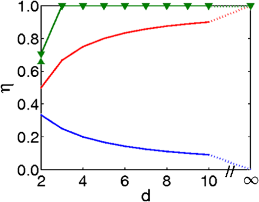
Figure 2: Parameter $\eta$ (see text) boundaries for Werner States. The blue line corresponds to $\eta=1/(d+1)$, the red line to $\eta=(1-d^{-1})$ and the green line to $\eta=1$ for $d\geq 3$. For $\eta$ below blue line the states are Category 1 - separable states. These states are also Bell local, LHS and non-steerable. For $\eta$ between blue line and red line the states are Category 2. These states are also Bell local, non-steerable and entangled. For $\eta$ between red line and green line the states are Category 3 - Bell local, steerable and entangled (EPR entangled). For $\eta$ above green line the states are Category 4 - Bell non-local, steerable and entangled. This is only possible for $d=2$. Figure taken from Wiseman et al. Ref. Wiseman07a .

Appendix F Idea of EPR Steering

In this Appendix we consider for reasons of completeness the physical idea behind EPR steering, as presented in the papers Wiseman07a ; Jones07a ; Cavalcanti09a .

We can derive expressions within LHV theory for the conditional probabilities defined in (87). These expressions apply for all three Bell local categories considered here. We will focus on LHS states, which in terms of our LHVCS may be either in Category 1 or Category 2. We will initially consider the latter.

In the case of Category 2 states (which are LHS states) we obtain from (27) and (87)

$$P(\beta|\Omega_{B}||\alpha,\Omega_{A},c)=\frac{\sum_{\lambda}P(\alpha|\Omega_{A},c,\lambda)\,\text{Tr}_{B}((\widehat{\Pi}_{\beta}^{B})\widehat{\rho}^{B}(\lambda))}{\sum_{\lambda}P(\alpha|\Omega_{A},c,\lambda)\,P(\lambda|c)}$$ (128)

using (11) and (29).

It is also important to realise that these LHS model states are still related to an overall quantum state, but one which is non-separable since we cannot derive the density operator (20) for separable states from Category 2 expression (27) for the joint probability. For Category 2 LHS states, $P(\alpha|\Omega_{A},c,\lambda)$ is not given by a quantum expression. However, as in Jones07a ; Cavalcanti09a we can relate the quantities in the LHS model (27) to a density operator for sub-system $B$ that is conditional on the results for measurements on sub-system $A$.

From (2) the quantum theory result for the probability that measurement of observable $\Omega_{A}$ results in outcome $\alpha$ is given by

$$P(\alpha|\Omega_{A},\rho)=\text{Tr}((\widehat{\Pi}_{\alpha}^{A}\otimes\widehat{1}^{B})\,\widehat{\rho}),$$ (129)

where $\widehat{\rho}$ is the density operator for the overall quantum state (the preparation symbol $c$ is left out for simplicity). In the Copenhagen interpretation of quantum theory the normalised state that is produced as a result of this measurement is the conditional state

$$\widehat{\rho}_{cond}(\alpha|\Omega_{A},\rho) = (\widehat{\Pi}_{\alpha}^{A}\otimes\widehat{1}^{B})\,\widehat{\rho}\,(\widehat{\Pi}_{\alpha}^{A}\otimes\widehat{1}^{B})/P(\alpha|\Omega_{A},\rho).$$

This state has a trace of unity, as required. To confirm that $\widehat{\rho}_{cond}(\alpha|\Omega_{A},\rho)$ does lead to the correct quantum expression for the conditional probability $P(\beta|\Omega_{B}||\alpha|\Omega_{A},\rho)$ (i.e. that measurement of $\Omega_{B}$ in sub-system $B$ will result in outcome $\beta$ given that measurement of $\Omega_{A}$ resulted in outcome $\alpha$ based on the quantum state $\widehat{\rho}$), we calculate the probability of that measurement of $\Omega_{B}$ in sub-system $B$ which will result in outcome $\beta$ for the quantum state $\widehat{\rho}_{cond}(\alpha|\Omega_{A},\rho)$. This is given by

$$P(\beta|\Omega_{B},\rho_{cond}) =\text{Tr}((\widehat{1}^{A}\otimes\widehat{\Pi}_{\beta}^{B})\,\widehat{\rho}_{cond}(\alpha|\Omega_{A},\rho)),$$

$$=\text{Tr}((\widehat{\Pi}_{\alpha}^{A}\otimes\widehat{\Pi}_{\beta}^{B})\widehat{\rho}(\widehat{\Pi}_{\alpha}^{A}\otimes\widehat{1}^{B}))/P(\alpha|\Omega_{A},\rho),$$

$$=\text{Tr}\left((\widehat{\Pi}_{\alpha}^{A}\otimes\widehat{\Pi}_{\beta}^{B})\,\widehat{\rho}\right)/P(\alpha|\Omega_{A},\rho),$$

$$=P(\alpha,\beta|\Omega_{A},\Omega_{B},\rho)/P(\alpha|\Omega_{A},\rho),$$

$$=P(\beta|\Omega_{B}\,||\alpha|\Omega_{A},\rho),$$ (131)

using the cyclic properties of the trace and $(\widehat{\Pi}_{\alpha}^{A})^{2}=\widehat{\Pi}_{\alpha}^{A}$, with the last line (see (87)) following from Bayes’ theorem. This confirms the status of $\widehat{\rho}_{cond}(\alpha|\Omega_{A},\rho)$.

The physical concept of steering has been discussed in several papers, including Wiseman07a ; Jones07a and Cavalcanti09a and was originally introduced by Schrödinger Schrodinger35a following the important EPR paper Einstein35a . The key idea is that when a measurement of $\Omega_{A}$ is made on sub-system $A$ resulting in outcome $\alpha$ (the bipartite quantum state prepared being $\rho$ ) this results in both the overall quantum state changing to a new conditioned state $\widehat{\rho}_{cond}(\alpha|\Omega_{A},\rho)$ (given in Eq. (LABEL:Eq.CondQState)) and hence the post-measurement state describing sub-system $B$ changing to

$$\widehat{\rho}_{cond}(\alpha|\Omega_{A},\rho)^{B}=\text{Tr}_{A}(\widehat{\rho}_{cond}(\alpha|\Omega_{A},\rho))$$ (132)

from its pre-measurement state $\widehat{\rho}^{B}=\text{Tr}_{A}(\widehat{\rho})$ given by the reduced density operator (Eq. 3). This strange quantum effect allows for an experiment carried out on sub-system $A$ to instantly change (or “steer”) the quantum state for sub-system $B$ into a new quantum state, even when the two sub-systems are localised in well-separated spatial regions and the experimenter on $A$ may have no direct access to sub-system $B$. For those who accept the Copenhagen interpretation of quantum theory there is nothing really strange involved. Quantum states merely specify all that can be known about the physical state (and no distinction between “physical state” and “quantum state” is made), so as the measurement of $\Omega_{A}$ has led to a particular outcome $\alpha$ our knowledge about the state has changed, and hence the quantum state for both the overall system and its sub-systems should change accordingly. Using quantum theory we can obtain an explicit formula for $\widehat{\rho}_{cond}(\alpha|\Omega_{A},\rho)^{B}$ and this is

$$\widehat{\rho}_{cond}(\alpha|\Omega_{A},\rho)^{B}= \sum\limits_{\beta l,\gamma n}\left|B\beta l\right\rangle\left\langle B\gamma n\right|$$

$$\times\sum\limits_{i}\,\rho_{A\alpha i,B\beta l::A\alpha i,B\gamma n}\,,$$ (133)

where the original density operator $\rho$ is expressed in terms of orthonormal basis states $\left|A\alpha i\right\rangle\otimes\left|B\beta n\right\rangle$ that are eigenstates for $\widehat{\Omega}_{A}$ and $\widehat{\Omega}_{B}$, with $i=1,2,..,d_{\alpha}$ and $n=1,2,..,d_{\beta}$ allowing for degeneracy.

We can also show that the sum of the conditional density operators $\widehat{\rho}_{cond}(\alpha|\Omega_{A},\rho)^{B}$ each weighted by the probability $P(\alpha|\Omega_{A},\rho)$ for the measurement outcome $\alpha$ for $\Omega_{A}$ gives the reduced density operator $\widehat{\rho}^{B}$ associated with the original state $\rho$. This result is not surprising, since carrying out the measurement of any choice of $\Omega_{A}$ and then discarding the results would be described by reduced density operator:

$$\sum\limits_{\alpha}P(\alpha|\Omega_{A},\rho)\,\widehat{\rho}_{cond}(\alpha|\Omega_{A},\rho)^{B}=\widehat{\rho}^{B}=\text{Tr}_{A}\widehat{\rho}.$$ (134)

The proofs of (133) and (134) are straightforward.

Thus, we have seen how according to quantum theory the quantum state describing sub-system $B$ changes as a result of measuring $\Omega_{A}$ on sub-system $A$ and obtaining outcome $\alpha$. Furthermore, we have obtained quantum theory expressions (131) for the conditional probability $P(\beta|\Omega_{B},\,\rho_{cond})$ for measurement of $\Omega_{B}$ on sub-system $B$ and obtaining outcome $\beta$ when measurement of $\Omega_{A}$ on sub-system $A$ resulted in outcome $\alpha$ and (133) for the quantum state describing sub-system $B$. The question then is: Although quantum theory gives the correct results for the conditional probability $P(\beta|\Omega_{B},\,\rho_{cond})$, can the same results also be explained in a local hidden variable theory?

Following the operational definition for steering in Refs. Wiseman07a ; Jones07a and Cavalcanti09a , the quantum state $\rho$ is only considered to be EPR steerable when the conditional probability $P(\beta|\Omega_{B}||\alpha,\Omega_{A},c)$ can not be explained via a local hidden variable theory. For the LHS cases of Category 1 and Category 2 states we will see that a LHV theory explanation applies. We consider what expression for a density operator for sub-system $B$ would give the LHS result for the conditional probability $P(\beta|\Omega_{B}||\alpha,\Omega_{A},c)$ for measurement of $\Omega_{B\text{ }}$to have outcome $\beta$, given that measurement of $\Omega_{A\text{ }}$has outcome $\alpha$ and the preparation process is $c$. In the case of Category 2 states we use Eqs. (27) and (29) in conjunction with (87) and (11) to find

$$P(\beta|\Omega_{B} ||\alpha,\Omega_{A},c)=$$

$$\frac{\sum\limits_{\lambda}P(\alpha|\Omega_{A},c,\lambda)\,\text{Tr}_{B}((\widehat{\Pi}_{\beta}^{B})\widehat{\rho}^{B}(\lambda))\,P(\lambda|c)\,}{\sum_{\lambda}P(\alpha|\Omega_{A},c,\lambda)\,P(\lambda|c)\,}.$$

We then define a new normalised quantum state for sub-system $B$, $\widehat{\rho}_{cond}^{B}(\alpha|\Omega_{A},c)$, by the expression

$$\widehat{\rho}_{cond}^{B}(\alpha|\Omega_{A},c) = \frac{\sum\limits_{\lambda}P(\alpha|\Omega_{A},c,\lambda)\,\widehat{\rho}^{B}(\lambda)\,P(\lambda|c)\,}{\text{Tr}_{B}\left(\sum\limits_{\lambda}P(\alpha|\Omega_{A},c,\lambda)\,\widehat{\rho}^{B}(\lambda)\,P(\lambda|c)\,\right)},$$ (136)

$$= \frac{\sum\limits_{\lambda}P(\alpha|\Omega_{A},c,\lambda)\,\widehat{\rho}^{B}(\lambda)\,P(\lambda|c)\,}{\left(\sum\limits_{\lambda}P(\alpha|\Omega_{A},c,\lambda)\,P(\lambda|c)\,\right)}.$$

It is to be noted that this state for sub-system $B$ involves local HVT and not quantum expressions for the measurement probabilities $P(\alpha|\Omega_{A},c,\lambda)$ for sub-system $A$. We then see from (2) that for this state the probability for measurement of $\Omega_{B\text{ }}$to have outcome $\beta$ is given by

$$\text{Tr}_{B}(\widehat{\Pi}_{\beta}^{B}\, \widehat{\rho}_{cond}^{B}(\alpha|\Omega_{A},c))$$

$$=\frac{\sum\limits_{\lambda}P(\alpha|\Omega_{A},c,\lambda)\,\text{Tr}_{B}((\widehat{\Pi}_{\beta}^{B})\widehat{\rho}^{B}(\lambda))\,P(\lambda|c)\,}{\sum\limits_{\lambda}P(\alpha|\Omega_{A},c,\lambda)\,P(\lambda|c)},$$

$$=P(\beta|\Omega_{B}||\alpha,\Omega_{A},c),$$ (137)

which is the same as (128) obtained for the Category 2 states (which are LHS states). Thus the sub-system $B$ quantum state (136) has been constructed purely from the Category 2 LHS model probabilities $P(\alpha|\Omega_{A},c,\lambda)\,$and $P(\lambda|c)$, together with the LHS model quantum state $\widehat{\rho}^{B}(\lambda)$ - which is a possible quantum state for sub-system $B$ based on hidden variables $\lambda$. The sub-system $B$ quantum state $\widehat{\rho}_{cond}^{B}(\alpha|\Omega_{A},c)$ in (136) determines the correct probability for measurement of $\Omega_{B\text{ }}$to have outcome $\beta$. The same analysis would apply to the LHS states in Category 1, the only difference being that $P(\alpha|\Omega_{A},c,\lambda)$ would be replaced by $P_{Q}(\alpha|\Omega_{A},c,\lambda)$ in terms of our notation. So in both of these cases there could be a hidden state $\widehat{\rho}^{B}(\lambda)$ associated with hidden variables that could explain (along with suitable choices for $P(\alpha|\Omega_{A},c,\lambda)\,$and $P(\lambda|c)$) the measurements on sub-system $B$. The treatment however does not apply to the quantum states in Category 3, where the LHV model in Eq. (28) does not include a quantum state $\widehat{\rho}^{B}(\lambda)$ for sub-system $B$. Hence, the conditional probability $P(\beta|\Omega_{B}||\alpha,\Omega_{A},c)$ can be explained via the LHS model for both Category 1 and Category 2 states, showing that the Category 1 and Category 2 quantum states are non-steerable. However, the Category 3 states are EPR steerable.

Appendix G Spin Variances: EPR Steering Test

The EPR steering test in (73) can be obtained from the results in Sections IV.5 and IV.6 by using (61), (45) and (54). We find using LHVT that for Category 2 states

$$\left\langle\Delta S_{x}^{2}\right\rangle+\left\langle\Delta S_{y}^{2}\right\rangle -\frac{1}{4}\left\langle N\right\rangle+\frac{1}{2}\left\langle S_{z}\right\rangle$$

$$\geq\left\langle N_{A}\otimes N_{B}\right\rangle+\frac{1}{2}\left\langle 1_{A}\otimes N_{B}\right\rangle,$$

$$\geq 0.$$ (138)

Details are:

$$\left\langle\Delta S_{x}^{2}\right\rangle +\left\langle\Delta S_{y}^{2}\right\rangle-\frac{1}{4}\left\langle N\right\rangle+\frac{1}{2}\left\langle S_{z}\right\rangle$$

$$\geq \left\langle N_{A}\otimes N_{B}\right\rangle+\frac{1}{2}\left\langle 1_{A}\otimes N_{B}\right\rangle+\frac{1}{2}\left\langle N_{A}\otimes 1_{B}\right\rangle$$

$$-\frac{1}{4}\left\langle 1_{A}\otimes N_{B}\right\rangle-\frac{1}{4}\left\langle N_{A}\otimes 1_{B}\right\rangle$$

$$+\frac{1}{4}\left\langle 1_{A}\otimes N_{B}\right\rangle-\frac{1}{4}\left\langle N_{A}\otimes 1_{B}\right\rangle,$$

$$\geq \left\langle N_{A}\otimes N_{B}\right\rangle+\frac{1}{2}\left\langle 1_{A}\otimes N_{B}\right\rangle,$$

$$\geq 0.$$ (139)

As LHVT is required to predict the same result as quantum theory we have

$$\left\langle\Delta\widehat{S}_{x}^{2}\right\rangle+\left\langle\Delta\widehat{S}_{y}^{2}\right\rangle -\frac{1}{4}\left\langle\widehat{N}\right\rangle+\frac{1}{2}\left\langle\widehat{S}_{z}\right\rangle$$

$$\geq \left\langle\widehat{N}_{A}\otimes\widehat{N}_{B}\right\rangle+\frac{1}{2}\left\langle\widehat{1}_{A}\otimes\widehat{N}_{B}\right\rangle,$$

$$\geq 0,$$ (140)

since both $\langle\widehat{N}_{A}\otimes\widehat{N}_{B}\rangle$ and $\langle\widehat{1}_{A}\otimes\widehat{N}_{B}\rangle$ are positive quantities. In this form it shows that if $\langle\Delta\widehat{S}_{x}^{2}\rangle+\langle\Delta\widehat{S}_{y}^{2}\rangle-\frac{1}{4}\langle\widehat{N}\rangle+\frac{1}{2}\langle\widehat{S}_{z}\rangle<0$ then the state cannot be Category 2. This result is also obtained by Appendices I and J.

Appendix H Variances of Two Mode Quadratures - Category 2 States

Using the LHVT expressions (46,LABEL:Eq.TwoModeQuadObservSquare) for $X_{\theta}(\pm)$ and $X_{\theta}(\pm)^{2}$ together with the results (49) and (58) for $\left\langle x_{B}\right\rangle$, $\left\langle p_{B}\right\rangle$ and $\left\langle U_{B}\right\rangle$, together with $U_{A}=\frac{1}{2}(x_{A}p_{A}+p_{A}x_{A})$, we find for Category 2 states the mean values of the two mode quadratures and their square are given by

$$\left\langle X_{\theta}(\pm)\right\rangle= \frac{1}{\sqrt{2}}\left(\left\langle x_{A}\right\rangle\cos\theta+\left\langle p_{A}\right\rangle\sin\theta\right),$$ (141)

$$\left\langle X_{\theta}(\pm)\right\rangle^{2}= \frac{1}{2}\big{(}\left\langle x_{A}\right\rangle^{2}\cos^{2}\theta+\left\langle p_{A}\right\rangle^{2}\sin^{2}\theta$$

$$~{}~{}~{}+2\left\langle x_{A}\right\rangle\left\langle p_{A}\right\rangle\sin\theta\cos\theta\big{)},$$

$$\left\langle X_{\theta}(\pm)^{2}\right\rangle= \frac{1}{2}\big{(}\left\langle x_{A}^{2}\right\rangle\cos^{2}\theta+\left\langle(x_{A}p_{A}+p_{A}x_{A})\right\rangle\sin\theta\cos\theta$$

$$~{}~{}~{}+\left\langle p_{A}^{2}\right\rangle\sin^{2}\theta\big{)}$$

$$+\frac{1}{2}\left(\left\langle N_{B}\right\rangle+\frac{1}{2}\right).$$ (142)

The variance for Category 2 states is then given by the LHVT expression

$$\left\langle\Delta X_{\theta}(\pm)^{2}\right\rangle =\frac{1}{2}\big{\langle}\left(\Delta x_{A}\cos\theta+\Delta p_{A}\sin\theta\right)$$

$$\qquad\times\left(\Delta x_{A}\cos\theta+\Delta p_{A}\sin\theta\right)\big{\rangle}$$

$$\quad+\frac{1}{2}\left(\left\langle N_{B}\right\rangle+\frac{1}{2}\right),$$

$$\left\langle\Delta P_{\theta}(\pm)^{2}\right\rangle =\frac{1}{2}\big{\langle}\left(-\Delta x_{A}\sin\theta+\Delta p_{A}\cos\theta\right)$$

$$\qquad\times\left(-\Delta x_{A}\sin\theta+\Delta p_{A}\cos\theta\right)\big{\rangle}$$

$$\quad+\frac{1}{2}\left(\left\langle N_{B}\right\rangle+\frac{1}{2}\right),$$ (143)

where $\Delta x_{A}=x_{A}-\left\langle x_{A}\right\rangle$ and $\Delta p_{A}=p_{A}-\left\langle p_{A}\right\rangle$. The expression for $\left\langle\Delta P_{\theta}(\pm)^{2}\right\rangle$ is obtained using $P_{\theta}(\pm)=X_{\theta+\pi/2}(\pm)$.

As LHVT underlies quantum theory then we also have for the quantum theory treatment of Category 2 states

$$\left\langle\Delta\widehat{X}_{\theta}(\pm)^{2}\right\rangle =\frac{1}{2}\big{\langle}\left(\Delta\widehat{x}_{A}\cos\theta+\Delta\widehat{p}_{A}\sin\theta\right)$$

$$\qquad\times\left(\Delta\widehat{x}_{A}\cos\theta+\Delta\widehat{p}_{A}\sin\theta\right)\big{\rangle}$$

$$\quad+\frac{1}{2}\left(\left\langle\widehat{1}_{A}\otimes\widehat{N}_{B}\right\rangle+\frac{1}{2}\right),$$ (144)

where now $\Delta\widehat{x}_{A}=\widehat{x}_{A}-\left\langle\widehat{x}_{A}\right\rangle$, $\Delta\widehat{p}_{A}=\widehat{p}_{A}-\left\langle\widehat{p}_{A}\right\rangle$. However, we can make use of the SSR to simplify these expressions further. As shown in SubSection II.1 the reduced density operator for sub-system $A$ satisfies the local particle number SSR. This is the case even though the reduced density operator depends on the full density matrix for both sub-systems, unlike that for a local hidden state. Consequently

$$\left\langle\widehat{x}_{A}\right\rangle =\text{Tr}_{A}(\widehat{x}_{A}\widehat{\rho}^{A})=0, \left\langle\widehat{p}_{A}\right\rangle =\text{Tr}_{A}(\widehat{p}_{A}\widehat{\rho}^{A})=0,$$

(145)

using the same arguments as for $\left\langle x_{B}(\lambda)\right\rangle_{Q}$ and $\left\langle p_{B}(\lambda)\right\rangle_{Q}$ in Eq. (49). Furthermore, the same steps as for $\left\langle x_{B}^{2}(\lambda)\right\rangle_{Q}$, $\left\langle p_{B}^{2}(\lambda)\right\rangle_{Q}$ and $\left\langle U_{B}(\lambda)\right\rangle_{Q}$ lead to

$$\left\langle\widehat{x}_{A}^{2}\right\rangle =\left\langle\widehat{N}_{A}\right\rangle+\frac{1}{2}, \left\langle\widehat{p}_{A}^{2}\right\rangle =\left\langle\widehat{N}_{A}\right\rangle+\frac{1}{2},$$

$$\left\langle\widehat{U}_{A}\right\rangle =0,$$ (146)

(see SubSubSection IV.5.3). Using these results we then find that

$$\left\langle\Delta\widehat{X}_{\theta}(\pm)^{2}\right\rangle =\frac{1}{2}\left(\left\langle\widehat{N}_{A}\otimes\widehat{1}_{B}\right\rangle+\frac{1}{2}\right)$$

$$\quad+\frac{1}{2}\left(\left\langle\widehat{1}_{A}\otimes\widehat{N}_{B}\right\rangle+\frac{1}{2}\right),$$

$$=\frac{1}{2}\left\langle\widehat{N}\right\rangle+\frac{1}{2},$$

$$\left\langle\Delta\widehat{P}_{\theta}(\pm)^{2}\right\rangle =\frac{1}{2}\left\langle\widehat{N}\right\rangle+\frac{1}{2}.$$ (147)

(The calculation for $\langle\Delta\widehat{P}_{\theta}(\pm)^{2}\rangle$ is trivial, as $\widehat{P}_{\theta}(\pm)=\widehat{X}_{\theta+\pi/2}(\pm)$). Exactly the same results apply for Category 1 (separable) states (see Appendix L in Ref. Dalton16b ).

Appendix I Correlation Tests for EPR Steering

The paper by Cavalcanti et al. Cavalcanti11a derives certain inequalities for $|\langle\widehat{a}^{{\dagger}}\widehat{b}\rangle|^{2}$ for Category 1 and Category 2 states which lead to strong correlation tests for EPR steering. We will show here that these inequalities lead to more useful tests in terms of spin operators for quantum entanglement and EPR steering. These inequalities are set out here in Eqs. (156) and (158) for Category 1 and Category 2 states respectively. The inequality in Eq. (156) has also been previously obtained for separable states by Hillery and Zubairy Hillery06a . They two inequalities correspond to Eqs. (15) and (14) in Ref. Cavalcanti11a where there are $N=2$ sub-systems (“sites”), with Eq. (15) applying when both sub-systems are associated with a LHS ($T=2$ - two “trusted sites”) and Eq. (14) when only one sub-system has a LHS ($T=1$ - one “trusted site”). The inequalities obtained by Cavalcanti et al Cavalcanti11a were based on their general expression in Eq. (4) for the LHV theory joint measurement probability, for which Eqs. (26) and (27) for Category 1 and Category 2 states are special cases. Hence these inequalities would apply for the present paper. For completeness however, rather than just quoting the inequalities in Ref. Cavalcanti11a we will also derive them here using the approach set out in the present paper. A further inequality for $|\langle\widehat{a}^{{\dagger}}\widehat{b}\rangle|^{2}$ will also be derived that would apply to Category 3 states.

For Category 1 states the result gives a strong correlation test and the Hillery-Zubairy Hillery06a test for quantum entanglement, whilst for Category 2 states the result gives a strong correlation test plus a generalised Hillery-Zubairy test for EPR steering, originally set out in He et al. He12a for the case where $\langle\widehat{S}_{z}\rangle=0$. The new test allows for $\langle\widehat{S}_{z}\rangle\neq 0$. For Category 3 states no useful test for Bell non-locality occurs.

I.1 General Correlation Inequality for $|\langle\widehat{a}^{{\dagger}}\widehat{b}\rangle|^{2}$: Bell Local States

Using Eqs. (33,LABEL:Eq.SpinCompts) to introduce quadrature operators and spin operators, the quantity $\widehat{a}^{{\dagger}}\widehat{b}$ can be written as

$$\widehat{a}^{{\dagger}}\widehat{b} = \frac{1}{2}(\widehat{x}_{A}-i\widehat{p}_{A})(\widehat{x}_{B}+i\widehat{p}_{B})$$ (148)

$$= \widehat{S}_{x}-i\widehat{S}_{y}$$

so that the LHVT quantity $\left\langle a^{{\dagger}}b\right\rangle$ becomes

$$\left\langle a^{{\dagger}}b\right\rangle=\frac{1}{2}\left(\left\langle x_{A}x_{B}\right\rangle+\left\langle p_{A}p_{B}\right\rangle+i\left(\left\langle x_{A}p_{B}\right\rangle-\left\langle p_{A}x_{B}\right\rangle\right)\right).$$ (149)

Then introducing the LHVT expression

$$\left\langle a^{{\dagger}}b\right\rangle=\frac{1}{2}\sum_{\lambda}P(\lambda|c)\left(\left\langle x_{A}(\lambda)\right\rangle-i\left\langle p_{A}(\lambda)\right\rangle\right)\\ \times\left(\left\langle x_{B}(\lambda)\right\rangle+i\left\langle p_{B}(\lambda)\right\rangle\right),$$

and

$$\left|\left\langle a^{{\dagger}}b\right\rangle\right|\leq\frac{1}{2}\sum_{\lambda}P(\lambda|c)|\left(\left\langle x_{A}(\lambda)\right\rangle-i\left\langle p_{A}(\lambda)\right\rangle\right)|\\ \times|\left(\left\langle x_{B}(\lambda)\right\rangle+i\left\langle p_{B}(\lambda)\right\rangle\right)|$$

with $|\left(\left\langle x_{A}(\lambda)\right\rangle-i\left\langle p_{A}(\lambda)\right\rangle\right)|=\sqrt{\left\langle x_{A}(\lambda)\right\rangle^{2}+\left\langle p_{A}(\lambda)\right\rangle^{2}}$ etc., we then find that

$$|\left\langle a^{{\dagger}}b\right\rangle|^{2}\;\leq\frac{1}{4}\Biggl{(}\sum_{\lambda}P(\lambda|c)\sqrt{\left\langle x_{A}(\lambda)\right\rangle^{2}+\left\langle p_{A}(\lambda)\right\rangle^{2}}\\ \times\sqrt{\left\langle x_{B}(\lambda)\right\rangle^{2}+\left\langle p_{B}(\lambda)\right\rangle^{2}}\Biggr{)}^{2}.$$ (150)

Using the inequality (32) with

$$C(\lambda)=\left(\left\langle x_{A}(\lambda)\right\rangle^{2}+\left\langle p_{A}(\lambda)\right\rangle^{2}\right)\\ \times\left(\left\langle x_{B}(\lambda)\right\rangle^{2}+\left\langle p_{B}(\lambda)\right\rangle^{2}\right)\geq 0,$$

we then have the key inequality

$$\left|\left\langle a^{{\dagger}}b\right\rangle\right|^{2}\;\leq\frac{1}{4}\sum_{\lambda}P(\lambda|c)\,\left(\left\langle x_{A}(\lambda)\right\rangle^{2}+\left\langle p_{A}(\lambda)\right\rangle^{2}\right)\\ \times\left(\left\langle x_{B}(\lambda)\right\rangle^{2}+\left\langle p_{B}(\lambda)\right\rangle^{2}\right)$$ (151)

that would follow from the approach in Ref. Cavalcanti11a . Again, as LHVT underlies quantum theory we can use (45), (60), (LABEL:Eq.MeanValueJointMeastsQThyLHVT), and (LABEL:Eq.MeanValueSingleMeastQThyLHVT) to write this inequality for all Bell local states in terms of quantum operators as

$$\left|\left\langle\widehat{a}^{{\dagger}}\widehat{b}\right\rangle\right|^{2} \leq\left\langle(\widehat{N}_{A}+\widehat{V}_{A})\otimes(\widehat{N}_{B}+\widehat{V}_{B})\right\rangle,$$

$$=\left\langle\widehat{N}_{A}\otimes\widehat{N}_{B}\right\rangle+\frac{1}{2}\left\langle\widehat{1}_{A}\otimes\widehat{N}_{B}\right\rangle$$

$$\quad+\frac{1}{2}\left\langle\widehat{N}_{A}\otimes\widehat{1}_{B}\right\rangle+\frac{1}{4}.$$ (152)

I.2 Stronger Correlation Inequalities for Bell Local States

Stronger inequalities can now be derived for the quantities $\langle x_{A}(\lambda)\rangle^{2}+\langle p_{A}(\lambda)\rangle^{2}$ and $\langle x_{B}(\lambda)\rangle^{2}+\langle p_{B}(\lambda)\rangle^{2}$ in the cases of Categories 1, 2 and 3 states. This leads to some outcomes different to (152).

Even if the sub-system $C$ does not involve a local hidden state $\widehat{\rho}_{\lambda}^{C}$ then we can always use the inequality (31) to give $\langle x_{C}(\lambda)\rangle^{2}\leq\langle x_{C}^{2}(\lambda)\rangle$ and $\langle p_{C}(\lambda)\rangle^{2}\leq\langle p_{C}^{2}(\lambda)\rangle$. This is equivalent to the variances of $x_{C}$ and $p_{C}$ being non-negative. Thus

$$\left\langle x_{C}\left(\lambda\right)\right\rangle^{2}+\left\langle p_{C}\left(\lambda\right)\right\rangle^{2}\leq\left\langle x_{C}^{2}(\lambda)\right\rangle+\left\langle p_{C}^{2}(\lambda)\right\rangle.$$ (153)

On the other hand, if the sub-system $C$ does involve a local hidden state $\widehat{\rho}_{\lambda}^{C}$ then we can obtain a stronger inequality via quantum theory. For any real $\eta$ the quantity $\left\langle\left(\Delta\widehat{x}_{C}-i\eta\Delta\widehat{p}_{C}\right)\left(\Delta\widehat{x}_{C}+i\eta\Delta\widehat{p}_{C}\right)\right\rangle_{\lambda}=\text{Tr}[\left(\Delta\widehat{x}_{C}-i\eta\Delta\widehat{p}_{C}\right)\left(\Delta\widehat{x}_{C}+i\eta\Delta\widehat{p}_{C}\right)\widehat{\rho}_{\lambda}^{C}]\geq 0$, where $\Delta\widehat{x}_{C}=\widehat{x}_{C}-\left\langle\widehat{x}_{C}\right\rangle_{\lambda}$, $\Delta\widehat{p}_{C}=\widehat{p}_{C}-\left\langle\widehat{p}_{C}\right\rangle_{\lambda}$. Thus for all $\eta$ we have $\left\langle\Delta\widehat{x}_{C}^{2}\right\rangle_{\lambda}-\eta+\eta^{2}\left\langle\Delta\widehat{p}_{C}^{2}\right\rangle_{\lambda}\geq 0$ using $[\widehat{x}_{C},\widehat{p}_{C}]=i$. Putting $\eta=1$ gives the inequality $\left\langle\Delta\widehat{x}_{C}^{2}\right\rangle_{\lambda}+\left\langle\Delta\widehat{p}_{C}^{2}\right\rangle_{\lambda}-1\geq 0$, which can be written as $\left\langle\widehat{x}_{C}\right\rangle_{\lambda}^{2}+\left\langle\widehat{p}_{C}\right\rangle_{\lambda}^{2}\leq\left\langle\widehat{x}_{C}^{2}\right\rangle_{\lambda}+\left\langle\widehat{p}_{C}^{2}\right\rangle_{\lambda}-1$. In terms of LHVT notation this inequality is

$$\left\langle x_{C}\left(\lambda\right)\right\rangle^{2}+\left\langle p_{C}\left(\lambda\right)\right\rangle^{2}\leq\left\langle x_{C}^{2}(\lambda)\right\rangle+\left\langle p_{C}^{2}(\lambda)\right\rangle-1.$$ (154)

For Category 1 states both sub-systems involve a local hidden state, so the key inequality (151) gives

$$|\left\langle a^{{\dagger}}b\right\rangle|^{2}\;\leq\frac{1}{4}\sum_{\lambda}P(\lambda|c)\,\left(\left\langle x_{A}^{2}(\lambda)\right\rangle+\left\langle p_{A}^{2}(\lambda)\right\rangle-1\right)\\ \times\left(\left\langle x_{B}^{2}(\lambda)\right\rangle+\left\langle p_{B}^{2}(\lambda)\right\rangle-1\right).$$ (155)

Using (LABEL:Eq.MeanValueJointMeastsQThyLHVT), (LABEL:Eq.MeanValueSingleMeastQThyLHVT), (36) and (35) we can then convert these inequalities to quantum expressions involving number operators, $\widehat{N}_{C}=\widehat{c}^{{\dagger}}\widehat{c}$ (where $C=A,B$):

$$\left|\left\langle\widehat{a}^{{\dagger}}\widehat{b}\right\rangle\right|^{2} \leq\left\langle\left(\widehat{N}_{A}+\widehat{V}_{A}-\widehat{1}_{A}/2\right)\otimes\left(\widehat{N}_{B}+\widehat{V}_{B}-\widehat{1}_{B}/2\right)\right\rangle,$$

$$=\left\langle\widehat{N}_{A}\otimes\widehat{N}_{B}\right\rangle.$$ (156)

For Category 2 states with sub-system $B$ involving a local hidden state $\widehat{\rho}_{\lambda}^{B}$, the key inequality (151) gives

$$\left|\left\langle a^{{\dagger}}b\right\rangle\right|^{2}\;\leq\frac{1}{4}\sum_{\lambda}P(\lambda|c)\,\left(\left\langle x_{A}^{2}(\lambda)\right\rangle+\left\langle p_{A}^{2}(\lambda)\right\rangle\right)\\ \times\left(\left\langle x_{B}^{2}(\lambda)\right\rangle+\left\langle p_{B}^{2}(\lambda)\right\rangle-1\right).$$ (157)

Similarly to the Category 1 case we then find that for Category 2 states (with $B$ involving the local hidden state)

$$\left|\left\langle\widehat{a}^{{\dagger}}\widehat{b}\right\rangle\right|^{2}\; \leq \left\langle\left(\widehat{N}_{A}+\widehat{V}_{A}\right)\otimes\left(\widehat{N}_{B}+\widehat{V}_{B}-\frac{1}{2}\widehat{1}_{B}\right)\right\rangle$$ (158)

$$= \left\langle\left(\widehat{N}_{A}+\frac{1}{2}\widehat{1}_{A}\right)\otimes\widehat{N}_{B}\right\rangle.$$

For Category 3 states with neither sub-system involving a local hidden state, the key inequality (151) gives

$$\left|\left\langle a^{{\dagger}}b\right\rangle\right|^{2}\;\leq\frac{1}{4}\sum_{\lambda}P(\lambda|c)\,\left(\left\langle x_{A}^{2}(\lambda)\right\rangle+\left\langle p_{A}^{2}(\lambda)\right\rangle\right)\\ \times\left(\left\langle x_{B}^{2}(\lambda)\right\rangle+\left\langle p_{B}^{2}(\lambda)\right\rangle\right).$$ (159)

In the case of the Category 3 states we then have

$$\left|\left\langle\widehat{a}^{{\dagger}}\widehat{b}\right\rangle\right|^{2}\; \leq \left\langle\left(\widehat{N}_{A}+\widehat{V}_{A}\right)\otimes\left(\widehat{N}_{B}+\widehat{V}_{B}\right)\right\rangle,$$

$$= \left\langle\left(\widehat{N}_{A}+\frac{1}{2}\widehat{1}_{A}\right)\otimes\left(\widehat{N}_{B}+\frac{1}{2}\widehat{1}_{B}\right)\right\rangle,$$

where we note that $\widehat{N}_{A}+\frac{1}{2}\widehat{1}_{A}=\widehat{a}^{{\dagger}}\widehat{a}+\frac{1}{2}=(\widehat{a}\widehat{a}^{{\dagger}}+\widehat{a}^{{\dagger}}\widehat{a})/2$. This result is the same as the general result (152) found for all Bell local states. Note also that this derivation of Eqs. (156,158) and (LABEL:Eq.IneqalCat3) did not make use of the SSR. Only the presence or absence of a local hidden state was invoked, and whether the LHS satisfied the SSR was not used.

As will be seen in the next Section, all these inequalities (156), (158) and (LABEL:Eq.IneqalCat3) can be expressed in terms of spin operator variances.

I.3 Correlations as Spin Operator Inequalities: Bell Local States

The inequalities (156,158) and (LABEL:Eq.IneqalCat3) derived above can be put into a more useful form involving spin operators - whose mean values and variances can be measured. From (148) we have (see also Ref. Dalton16b )

$$\left|\left\langle\widehat{a}^{{\dagger}}\widehat{b}\right\rangle\right|^{2} =\left\langle\widehat{S}_{x}\right\rangle^{2}+\left\langle\widehat{S}_{y}\right\rangle^{2},$$

$$\widehat{N}_{A} =\frac{1}{2}\widehat{N}-\widehat{S}_{z}, \widehat{N}_{B} =\frac{1}{2}\widehat{N}+\widehat{S}_{z},$$

$$\widehat{S}_{x}^{2}+\widehat{S}_{y}^{2}+\widehat{S}_{z}^{2} =\frac{\widehat{N}}{2}(\frac{\widehat{N}}{2}+1).$$ (161)

Then we find, after some straightforward calculations and introducing the variances $\langle\Delta\widehat{S}_{x}^{2}\rangle=\langle\widehat{S}_{x}^{2}\rangle-\langle\widehat{S}_{x}\rangle^{2}$ etc., the following results for Category 1, 2 and 3 states:

$$\left\langle\Delta\widehat{S}_{x}^{2}\right\rangle+\left\langle\Delta\widehat{S}_{y}^{2}\right\rangle-\frac{1}{2}\left\langle\widehat{N}\right\rangle \geq 0$$

Category 1 States (162)

$$\left\langle\Delta\widehat{S}_{x}^{2}\right\rangle+\left\langle\Delta\widehat{S}_{y}^{2}\right\rangle-\frac{1}{4}\left\langle\widehat{N}\right\rangle+\frac{1}{2}\left\langle\widehat{S}_{z}\right\rangle \geq 0$$

Category 2 States (163)

$$\left\langle\Delta\widehat{S}_{x}^{2}\right\rangle+\left\langle\Delta\widehat{S}_{y}^{2}\right\rangle+\frac{1}{4} \geq 0$$

Category 3 States (164)

Details are given in Appendix J. For Category 2 states with $A$ involving the LHS then the left side would have involved $-\frac{1}{2}\langle\widehat{S}_{z}\rangle$.

The inequality (163) for Category 2 states was obtained more directly without using the strong correlation inequalities in Sections IV.5, IV.6 - see Eqs. (61,67) and (54). Details were given in Appendix G. The inequality (162) for Category 1 states was also derived in Refs. Hillery06a and Dalton16b .

We note in passing that Eq. (164) does not lead to a test for Bell non-locality. From the Heisenberg Uncertainty Principle this inequality applies for all quantum states. Hence the inequalities (LABEL:Eq.IneqalCat3) or (164) do not provide a test for Bell non-locality.

I.4 Weak Correlation Test

The quantum operator $\widehat{a}^{{\dagger}}\widehat{b}$ is not an observable, but from the definitions for the spin operator we can write $\widehat{a}^{{\dagger}}\widehat{b}=\widehat{S}_{x}-i\widehat{S}_{y}$. We have interpreted $a^{{\dagger}}b$ to be $S_{x}-iS_{y}$, where now $S_{x}$ and $S_{y}$ are observables whose mean values are definable in a LHV theory.

From (115) and (52) we see that for Category 2 (and Category 1) states

$$\left\langle a^{{\dagger}}b\right\rangle = \left\langle S_{x}\right\rangle-i\left\langle S_{y}\right\rangle,$$ (165)

$$= 0,$$

so that

$$|\left\langle a^{{\dagger}}b\right\rangle|^{2}=\left\langle S_{x}\right\rangle^{2}+\left\langle S_{y}\right\rangle^{2}=0$$ (166)

for quantum states in Category 2 (or Category 1). This means that if

$$\left|\left\langle\widehat{a}^{{\dagger}}\widehat{b}\right\rangle\right|^{2}>0,$$ (167)

the state cannot be either Category 1 or Category 2. This constitutes a so-called weak correlation test for EPR steering. However because $|\langle\widehat{a}^{{\dagger}}\widehat{b}\rangle|^{2}=\langle\widehat{S}_{x}\rangle^{2}+\langle\widehat{S}_{y}\rangle^{2}$ this test is really just equivalent to the Bloch vector test. So no useful test for either quantum entanglement or EPR steering involving $\langle\widehat{S}_{x}\rangle^{2}+\langle\widehat{S}_{y}\rangle^{2}$ and $\langle\widehat{N}_{A}\otimes\widehat{N}_{B}\rangle$ is established at this point. However (see Section I.5) it was shown that related tests can be obtained both for quantum entanglement and EPR steering.

I.5 Strong Correlation Test

Hillery and Zubairy Hillery06a showed that for separable states (Category 1 states) that $|\langle\widehat{a}^{{\dagger}}\widehat{b}\rangle|^{2}\leq\langle\widehat{a}^{{\dagger}}\widehat{a}\widehat{b}^{{\dagger}}\widehat{b}\rangle=\langle\widehat{N}_{A}\otimes\widehat{N}_{B}\rangle$. This result is also obtained here in Eq. (156). The proof of this result was valid irrespective of whether the sub-system states $\widehat{\rho}_{R}^{A}$ and $\widehat{\rho}_{R}^{B}$ were local particle number SSR compliant or not (see Ref. Dalton16b for details). The quantum result

$$\left|\left\langle\widehat{a}^{{\dagger}}\widehat{b}\right\rangle\right|^{2} = \left\langle\widehat{S}_{x}\right\rangle^{2}+\left\langle\widehat{S}_{y}\right\rangle^{2},$$ (168)

$$> \left\langle\widehat{N}_{A}\otimes\widehat{N}_{B}\right\rangle,$$

is a strong correlation test for quantum entanglement. Hence as the numbers of bosons $N_{A}$ and $N_{B}$ are observables in the LHV model (and therefore the mean $\left\langle N_{A}\otimes N_{B}\right\rangle$ can be defined) we see that for Category 1 states the LHVT result

$$\left|\left\langle a^{{\dagger}}b\right\rangle\right|^{2}\leq\left\langle N_{A}\otimes N_{B}\right\rangle$$ (169)

applies. Thus if

$$\left|\left\langle\widehat{a}^{{\dagger}}\widehat{b}\right\rangle\right|^{2}>\left\langle\widehat{N}_{A}\otimes\widehat{N}_{B}\right\rangle,$$ (170)

we have a strong correlation test for entanglement. However, there is a different strong correlation test for EPR steering that applies - and which is harder to satisfy.

In the case of Category 2 states from the inequality in Eq. (158) we see that if

$$\left|\left\langle\widehat{a}^{{\dagger}}\widehat{b}\right\rangle\right|^{2}>\left\langle\widehat{N}_{A}\otimes\widehat{N}_{B}\right\rangle+\frac{1}{2}\left\langle\widehat{1}_{A}\otimes\widehat{N}_{B}\right\rangle,$$ (171)

the state cannot be in Category 2 (nor in Category 1) so it must be EPR steerable. Thus the inequality (171) is a strong correlation test for EPR steering. Note that the condition is harder to satisfy than the strong correlation test (168) for entanglement since $\langle\widehat{1}_{A}\otimes\widehat{N}_{B}\rangle$ is positive, but obviously if (171) is satisfied the state is entangled as well as being EPR steerable. If $A$ involved the LHS then the right side would have been $\langle\widehat{N}_{A}\otimes(\widehat{N}_{B}+\frac{1}{2}\widehat{1}_{B})\rangle$.

However, as these tests are just equivalent to the Hillery-Zubairy planar spin variance test and the generalised Hillery-Zubairy planar spin variance test, no additional test has been obtained.

Appendix J Correlation Inequalities and Spin Operators

The inequalities (156), (158) and (LABEL:Eq.IneqalCat3) derived above can be put into a more useful form involving spin operators - whose mean values and variances can be measured. We use the definitions of the spin operators in Section IV.3 (see also Ref. Dalton16b )

$$|\left\langle\widehat{a}^{{\dagger}}\widehat{b}\right\rangle|^{2} = \left\langle\widehat{S}_{x}\right\rangle^{2}+\left\langle\widehat{S}_{y}\right\rangle^{2},$$

$$\widehat{N}_{A} = \frac{1}{2}\widehat{N}-\widehat{S}_{z},\qquad\widehat{N}_{B}=\frac{1}{2}\widehat{N}+\widehat{S}_{z},$$

$$\widehat{S}_{x}^{2}+\widehat{S}_{y}^{2}+\widehat{S}_{z}^{2} = \frac{\widehat{N}}{2}(\frac{\widehat{N}}{2}+1).$$ (172)

We see that

$$\left\langle\Delta\widehat{S}_{x}^{2}\right\rangle+\left\langle\Delta\widehat{S}_{y}^{2}\right\rangle =\frac{1}{4}\left\langle(\widehat{N}_{A}+\widehat{N}_{B})^{2}\right\rangle+\frac{1}{2}\left\langle\widehat{N}_{A}+\widehat{N}_{B}\right\rangle$$

$$\quad-\left|\left\langle\widehat{a}^{{\dagger}}\widehat{b}\right\rangle\right|^{2}-\frac{1}{4}\left\langle(\widehat{N}_{B}-\widehat{N}_{A})^{2}\right\rangle,$$

$$\left\langle\Delta\widehat{S}_{x}^{2}\right\rangle+\left\langle\Delta\widehat{S}_{y}^{2}\right\rangle \geq\left\langle\widehat{N}_{A}\otimes\widehat{N}_{B}\right\rangle+\frac{1}{2}\left\langle\widehat{N}_{A}\otimes\widehat{1}_{B}\right\rangle$$

$$\quad+\frac{1}{2}\left\langle\widehat{1}_{A}\otimes\widehat{N}_{B}\right\rangle-\left\langle\widehat{N}_{A}\otimes\widehat{N}_{B}\right\rangle,$$

$$\geq\frac{1}{2}\left\langle\widehat{N}_{A}\otimes\widehat{1}_{B}\right\rangle+\frac{1}{2}\left\langle\widehat{1}_{A}\otimes\widehat{N}_{B}\right\rangle,$$

Cat 1 States

$$\left\langle\Delta\widehat{S}_{x}^{2}\right\rangle+\left\langle\Delta\widehat{S}_{y}^{2}\right\rangle \geq\left\langle\widehat{N}_{A}\otimes\widehat{N}_{B}\right\rangle+\frac{1}{2}\left\langle\widehat{N}_{A}\otimes\widehat{1}_{B}\right\rangle$$

$$\quad+\frac{1}{2}\left\langle\widehat{1}_{A}\otimes\widehat{N}_{B}\right\rangle$$

$$\quad-\left\langle\left(\widehat{N}_{A}+\frac{1}{2}\widehat{1}_{A}\right)\otimes\widehat{N}_{B}\right\rangle,$$

$$\geq\frac{1}{2}\left\langle\widehat{N}_{A}\otimes\widehat{1}_{B}\right\rangle,\qquad\text{Cat 2 States}$$

$$\left\langle\Delta\widehat{S}_{x}^{2}\right\rangle+\left\langle\Delta\widehat{S}_{y}^{2}\right\rangle \geq\left\langle\widehat{N}_{A}\otimes\widehat{N}_{B}\right\rangle+\frac{1}{2}\left\langle\widehat{N}_{A}\otimes\widehat{1}_{B}\right\rangle$$

$$\quad+\frac{1}{2}\left\langle\widehat{1}_{A}\otimes\widehat{N}_{B}\right\rangle$$

$$\quad-\left\langle\left(\widehat{N}_{A}+\frac{1}{2}\widehat{1}_{A}\right)\otimes\left(\widehat{N}_{B}+\frac{1}{2}\widehat{1}_{B}\right)\right\rangle,$$

$$\geq-\frac{1}{4}.\qquad\qquad\quad\text{Cat 3 States}$$ (173)

So we have:

$$\left\langle\Delta\widehat{S}_{x}^{2}\right\rangle+\left\langle\Delta\widehat{S}_{y}^{2}\right\rangle-\frac{1}{2}\left\langle\widehat{N}\right\rangle \geq 0\,,$$

Cat 1 States

$$\left\langle\Delta\widehat{S}_{x}^{2}\right\rangle+\left\langle\Delta\widehat{S}_{y}^{2}\right\rangle-\frac{1}{4}\left\langle\widehat{N}\right\rangle+\frac{1}{2}\left\langle\widehat{S}_{z}\right\rangle \geq 0\,,$$

Cat 2 States

$$\left\langle\Delta\widehat{S}_{x}^{2}\right\rangle+\left\langle\Delta\widehat{S}_{y}^{2}\right\rangle+\frac{1}{4} \geq 0\,.$$

Cat 3 States

References

• (1) B. J. Dalton, L. Heaney, J. Goold, B. M. Garraway and Th. Busch, New J. Phys. 16, 013026 (2014).
• (2) B. J. Dalton, J. Goold, B. M. Garraway and M. D. Reid, Phys. Scr. 92, 023004 (2017).
• (3) B. J. Dalton, J. Goold, B. M. Garraway and M. D. Reid, Phys. Scr. 92, 023005 (2017).
• (4) J. S. Bell, Physics 1, 195 (1964).
• (5) A. Einstein, B. Podolsky and N. Rosen, Phys. Rev. 47, 777 (1935).
• (6) H. M. Wiseman, S. J. Jones and A. C. Doherty, Phys. Rev. Lett. 98, 140402 (2007).
• (7) S. J. Jones, H. M. Wiseman and A. C. Doherty, Phys. Rev. A 76, 052116 (2007).
• (8) E. G. Cavalcanti, S. J. Jones, H. M. Wiseman and M. D. Reid, Phys. Rev. A 80, 032112 (2009).
• (9) S. Jevtic, M. J. W. Hall, M. R. Anderson, M. Zwierz and H. M. Wiseman, J. Opt. Soc. Am. B 32, A40 (2015).
• (10) E. Schrödinger, Proc. Camb. Phil. Soc. 31, 555 (1935); Proc. Camb. Phil. Soc. 32, 446 (1936).
• (11) E. Schrödinger, Naturwissenschaften 23, 807 (1935).
• (12) R. F. Werner, Phys. Rev. A 40, 4277 (1989).
• (13) Q. Y. He, P. D. Drummond, and M. D. Reid, Phys. Rev. A 83, 032120 (2011).
• (14) M. Hillery and M. S. Zubairy, Phys. Rev. Lett. 96, 050503 (2006).
• (15) Q. Y. He, P. D. Drummond, M. K. Olsen and M. D. Reid, Phys. Rev. A 86, 023626 (2012).
• (16) E. G. Cavalcanti, Q. Y. He, M. D. Reid. and H. M. Wiseman, Phys. Rev. A 84, 032115 (2011).
• (17) C. Gross, T. Zibold, E. Nicklas, J. Estève and M. K. Oberthaler, Nature 464, 1165 (2010).
• (18) M. F. Riedel, P. Böhi, Y. Li, T. W. Hänsch, A. Sinatra and P. Treutlein, Nature 464, 1170 (2010).
• (19) K. Maussang, G. E. Marti, T. Schneider, P. Treutlein, Y. Li, A. Sinatra, R. Long, J. Estève, and J. Reichel, Phys. Rev. Lett. 105, 080403 (2010).
• (20) M. Egorov, R. P. Anderson, V. Ivannikov, B. Opanchuk, P. Drummond, B. V. Hall and A. I. Sidorov, Phys. Rev. A 84, 021605 (2011).
• (21) C. Gross, H. Strobel, E. Nicklas, T. Zibold, N. Bar-Gill, G. Kurizki, and M. K. Oberthaler, Nature 480, 219 (2011).
• (22) J. Peise, I. Kruse, K. Lange, B. Lücke, L. Pezzè, J. Arlt, W. Ertmer, K. Hammerer, L. Santos, A. Smerzi and C. Klempt, Nature Comm. 6, 8984 (2015).
• (23) P. Kunkel, M. Prüfer, H. Strobel, D. Linnemann, A. Frölian, T. Gasenzer, M. Gärttner, and M. K. Oberthaler, Science 360, 413 (2018).
• (24) M. Fadel, T. Zibold, B. Décamps, and P. Treutlein, Science 360, 409 (2018).
• (25) K. Lange, J. Peise, B. Lücke, I. Kruse, G. Vitagliano, I. Apellaniz, M. Kleinmann, G. Tóth, and C. Klempt, Science 360, 416 (2018).
• (26) M. D. Reid, P. D. Drummond, W. P. Bowen, E. G. Cavalcanti, P. K. Lam, H. A. Bachor, U. L. Andersen and G. Leuchs, Rev. Mod. Phys. 81, 1727 (2009).
• (27) J. F. Clauser, M. A. Horne, A. Shimony and R. A. Holt, Phys. Rev. Lett. 23, 880 (1969).
• (28) B. Opanchuk, L. Rosales-Zárate, R. Y. Teh, B. J. Dalton, A. I. Sidorov, P. Drummond and M. D. Reid, Phys. Rev. A 100, 060102(R) (2019).
• (29) L. Rosales-Zárate, B. J. Dalton and M. D. Reid, Phys. Rev. A 98, 022120 (2018).
• (30) D. Bohm, Quantum Theory, Prentice-Hill: New York, USA, 1951.
• (31) C. J. Isham, Lectures on Quantum Theory (Imperial College Press: London (1995)).
• (32) J. S. Bell, in Foundations of Quantum Mechanics - Proceedings of the International School of Physics ’Enrico Fermi’ Course II, Ed. B. D’Espagnat, (Academic, New York, USA, 1971) pp171 - 181.
• (33) N. Brunner, D. Cavalcanti, S. Pironio, V. Scarani and S. Wehner, Rev. Mod. Phys. 86, 419 (2014).
• (34) S. M. Barnett, Quantum Information (Oxford University Press: Oxford (2009)).
• (35) H. F. Hofmann and S. Takeuchi, Phys. Rev. A 68, 032103 (2003).