Atmospheric Habitable Zones in Cool Y Dwarf Atmospheres

Abstract

We use a simple organism lifecycle model to explore the viability of an atmospheric habitable zone (AHZ), with temperatures that could support Earth-centric life, which sits above an environment that does not support life. To illustrate our model we use a cool Y dwarf atmosphere, such as WISE J085510.83–0714442.5 whose 4.5–5.2 micron spectrum shows absorption features consistent with water vapour and clouds. We allow organisms to adapt to their atmospheric environment (described by temperature, convection, and gravity) by adopting different growth strategies that maximize their chance of survival and proliferation. We assume a constant upward vertical velocity through the AHZ. We found that the organism growth strategy is most sensitive to the magnitude of the atmospheric convection. Stronger convection supports the evolution of more massive organisms. For a purely radiative environment we find that evolved organisms have a mass that is an order of magnitude smaller than terrestrial microbes, thereby defining a dynamical constraint on the dimensions of life that an AHZ can support. Based on a previously defined statistical approach we infer that there are of order $10^{9}$ cool Y brown dwarfs in the Milky Way, and likely a few tens of these objects are within ten parsecs from Earth. Our work also has implications for exploring life in the atmospheres of temperate gas giants. Consideration of the habitable volumes in planetary atmospheres significantly increases the volume of habitable space in the galaxy.

1 Introduction

The recent discoveries of Earth-like planets orbiting their host stars outside our solar system are beginning to challenge our understanding of planetary formation and the development of extra-terrestrial life. A common definition of whether a planet is capable of supporting life is is whether the effective surface temperature can sustain liquid water at its surface, which reflects several factors including the evolution of the planet and star, and the distance between them (Kasting et al. 1993). Here, drawing on our knowledge of Earth and inspired by previous theoretical work for the Jovian atmosphere we argue that an atmosphere sitting above a potentially uninhabitable planetary surface may be cool enough to sustain life. By doing this we define an atmospheric habitable zone (AHZ).

The Earth’s atmosphere contains a large number of aerosolized microbes with concentrations ranging from $10^{3}~{}\mathrm{m}^{-3}$ to more than $10^{6}~{}\mathrm{m}^{-3}$ of air, of which approximately 20% are larger than $0.5~{}\mathrm{\mu m}$ (Bowers et al. 2012). The atmospheric residence time of these organisms is highly uncertain but there is a growing body of works that show that some organisms are metabolically active, particularly in clouds (Lighthart & Shaffer 1995; Lighthart 1997; Fuzzi et al. 1997; Sattler et al. 2001; Côté et al. 2008; Womack et al. 2010; Gandolfi et al. 2013). Other solar system planets have been postulated to have a habitable atmosphere. The Venusian surface temperature (${\sim}738$ K) is too high to sustain liquid water, so based on Earth-centric definitions it is uninhabitable. At the cloud deck at ${\sim}55$ km, where atmospheric temperatures are close to those at Earth’s surface, liquid water is more readily available and conditions are more amenable to sustaining life (Cockell 1999; Schulze-Makuch et al. 2004; Dartnell et al. 2015). The Jovian atmosphere has also been considered to be potentially habitable. Sagan & Salpeter (1976) described a microbial ecosystem that could optimize a survival strategy to take advantage of their physical environment.

To illustrate the idea of the AHZ we focus on cool, free-floating Y-class brown dwarfs (Kirkpatrick et al. 2012), thereby avoiding complications associated with any stellar effects on an atmosphere or on inhabiting organisms (e.g. radiation, stellar particles, and electromagnetic interactions). The coolest known object WISE J$085510.83-071442.5$ (henceforth W0855-0714) has a mass $M_{\mathrm{BD}}$ of $6.5\pm 3.5M_{\mathrm{Jup}}$, a radius $R_{\mathrm{BD}}$ equal to $R_{\mathrm{Jup}},6.99\times 10^{4}~{}\mathrm{km}$, and an effective temperature $T_{\mathrm{eff}}$ of ${\sim}250~{}\mathrm{K}$ (Beamín et al. 2014; Faherty et al. 2014; Kopytova et al. 2014; Luhman 2014). We expect that the upper atmosphere of cool objects similar to WISE0855-0714 will have values for temperature and pressure similar to Earth’s lower atmosphere, and models and the latest spectra have suggested that liquid water in clouds may also be present (Faherty et al. 2014; Morley et al. 2014a, b; Skemer et al. 2016). Observed spectra for cool brown dwarfs are consistent with significant dust loading in the upper atmosphere (Tsuji 2005; Witte et al. 2011). These aerosols can provide charged surfaces on which prebiotic molecules, necessary for life, could form (Stark et al. 2014). Prebiotic molecules could also be delivered to the brown dwarf atmosphere via dust from the interstellar medium (Muñoz Caro et al. 2002). Based on current understanding, M/L/T brown dwarf atmospheres also contain most of the elements that are thought to be necessary for life: C (in CH₄, CO, CO₂), H (CH₄, H₂, H₂O, NH₃, NH₄SH), N (N₂, NH₃), O (CO₂, CO, OH), and S (NH₄SH, Na₂S) (for example, see Allard et al. 2012; Cushing et al. 2004, 2006, 2007, 2011; Kirkpatrick et al. 2012).

We develop the idea of a cool brown dwarf atmospheric sustaining life in its atmosphere by using a simple 1-D model to describe the evolution of a microbial ecosystem, following Sagan & Salpeter (1976), that is subject to convection and gravitational settling. The simplicity of our approach allows us to develop a probabilistic understanding of the survival of individual organisms under different environmental conditions.

In the next section we describe our numerical models. In section 3 we present analytical and numerical results, including a small number of sensitivity experiment that test our prior assumptions. We discuss our results in a broader astrobiological context and conclude the paper in section 4.

2 Model Description

We develop a simple atmospheric model that retains a sufficient level of detail to describe the atmospheric environment that drives variations in the lifecycle of the organism population. The organism model draws from nutrient-phytoplankton models used to described ocean biology on Earth (e.g., Franks (2002)), but we allow organisms to determine an evolutionary growth strategy that is best suited to the atmospheric environment.

2.1 Brown Dwarf Atmosphere

As described above, our illustrative calculations are based loosely on the object W0855-0714 (Luhman 2014). We are interested in the region of the atmosphere that has temperatures in the range $258~{}\mathrm{K}<T<395~{}\mathrm{K}$, which represent the lower and upper limits for life on Earth (McKay 2014). We define the AHZ as the atmospheric region(s) that fall between those limits.

For our work, we define a $T-P$ profile based on the 200$~{}\mathrm{K}$, $\log g=5.0$ profile from the 1D model of Morley et al. (2014b), assuming an atmosphere composed of 85% H₂ and 15% He. We assume these gases exhibit near-ideal behaviour so we can calculate density using the ideal gas law and altitudes can be calculated from scale heights. We define altitude at the bottom of the AHZ as $0~{}\mathrm{km}$, and the P-T profile places upper edge of the AHZ at $\sim 105~{}\mathrm{km}$. We calculate the luminosity of the object using the Stefan-Boltzmann law and $T_{\mathrm{eff}}\sim 250K$ (Luhman 2014).

Our model atmosphere assumes the presence of liquid water in the AHZ to support the biochemistry necessary to sustain life, as we know it on Earth. This assumption restricts us to the coolest Y dwarfs and also, for example, some cool gas giants. To illustrate our AHZ hypothesis, we use a T–P (T_gas–P_gas) profile determined from a 1-D hydrostatic model atmosphere simulation for Y dwarfs (Morley et al. 2014a). This model assumes equilibrium condensation processes such that super saturation = 1. For a T_eff=200 K, $\log g$ = 5 object, the T–P profile places the water phase transition between gas/liquid and ice at a temperature lower than 273 K at 0.7 bar pressure (Morley et al. 2014a). To illustrate our model we use a cool Y dwarf atmosphere, for example WISE 0855-0714 whose 4.5-—5.2 micron spectrum shows absorption features consistent with water vapour and clouds (Skemer et al. 2016). A supporting model calculation for this object (T_eff=250 K) shows that the temperature profile intercepts the saturation vapour pressure at $\simeq$273 K (Skemer et al. 2016), assuming equilibrium condensation processes (Morley et al. 2014a). In nature, non-equilibrium processes (super saturation $>$ 1) compete with equilibrium processes, allowing liquid water to exist at super cooled (metastable) temperatures much lower than 273 K, e.g. Rogers & Yau (1995); Helling & Fomins (2013); Helling & Casewell (2014).

Homogeneous freezing of pure liquid water is due to statistical fluctuations of its molecular structure such that smaller drops ($<$5 microns) freeze spontaneously at temperatures closer to 243 K while larger droplets freeze at slightly higher temperatures (Rogers & Yau 1995); similar empirical results are found for heavy water (Wölk & Strey 2001). On Earth, liquid water is not commonly found at such low temperatures suggesting a role for heterogeneous freezing processes. Liquid clouds are more commonly found at 253 K (Rogers & Yau 1995). A cloud can be considered as a collection of independent liquid droplets such that each droplet must be subjected to a nucleation event before the whole cloud is frozen. A consequence of this is that mixed-phase clouds are common over the coldest (polar) geographical regions on Earth (Morrison et al. 2012; Lawson & Gettelman 2014; Loewe et al. 2016). Aerosols and aqueous solutions influence nucleation of ice. Aerosol particles can act as ice nuclei. Ice can form directly from the gas phase on suitable ice nuclei via deposition and freezing heterogeneous nucleation processes (Rogers & Yau 1995). Liquid water existing as a component of an aqueous solution can significantly affect the temperature at which ice begins to nucleate, depending on the water activity of the solution (Koop et al. 2000). Based on this we argue that homogeneous and heterogeneous nucleation processes allow liquid water to exist at temperatures much lower than 273 K. The lower limit for the AHZ temperature is, however, determined by the coldest temperature ($\sim 253~{}\mathrm{K}$) that can support Earth-based life.

For simplicity, we use a constant convective vertical velocity $v_{\mathrm{conv.}}$ throughout the AHZ. We use values of $v_{\mathrm{conv.}}$ taken from a 3-D model of atmospheric dynamics (Showman & Kaspi 2013), which was used to study L/T dwarfs. Because Y dwarfs are cooler we expect the associated convective velocities to be smaller. We use two values, $v_{\mathrm{conv.}}=100~{}\mathrm{cm~{}s^{-1}}$ and $v_{\mathrm{conv.}}=1000~{}\mathrm{cm~{}s^{-1}}$, which cover a range of plausible convection scenarios, to assess the effect of the windspeed on the final population of organisms. In addition we consider a radiative atmosphere, with $v_{\mathrm{conv.}}=0.01~{}\mathrm{cm~{}s^{-1}}$.

2.2 Model of Organisms and their Lifecycle

We describe an individual organism as a frictionless spherical shell, following Sagan & Salpeter (1976). The shell is described by its radius, skin width, mass, and density of the organic skin (Figure 1). Organisms increase their mass by consuming biomass, described below. Increasing an organism’s mass increases its size and skin width according to an organism-specific growth strategy, $G$, which is given by

$$w_{\mathrm{o}}=(1-G)R_{\mathrm{o}},$$ (1)

where $w_{\mathrm{o}}$ is the organic skin thickness, and $R_{\mathrm{o}}$ is the radius of the sphere. Thus an individual organism with $G\rightarrow 1$ is balloon-like, whilst organisms with $G\rightarrow 0$ are solid throughout. We limit the skin densities $\rho_{\mathrm{o}}$ to range between $0.5~{}\mathrm{g~{}cm^{-3}}<\rho_{\mathrm{o}}<1.5~{}\mathrm{g~{}cm^{-3}}$. This is equivalent to densities greater than some light woods and less than the density of heavy woods and bone. As a comparisons, humans and microbes are approximately $1.0~{}\mathrm{g~{}cm^{-3}}$, the density of water, reflecting their bulk composition. For the purpose of this paper we assume this skin is permeable so that the density of the organism within the skin is the same at the atmosphere $\rho_{o}$. At the start of each experiment organisms are uniformally distributed throughout the AHZ.

Figure 1: Schematic of a model organism. The thickness and density of the organic skin layer are denoted by $w_{0}$ and $\rho_{0}$, respectively. The radius of the shell is denoted by $R_{0}$ and the density of the gas within the skin, in equilbrium with the atmosphere, is denoted by $\rho_{\mathrm{gas}}$. The upward velocity is denoted by $v_{\mathrm{conv.}}$ and the terminal velocity due to gravity is denoted by $v_{\mathrm{grav.}}$.

Each organism has a lifecycle of growth, reproduction (subject to sufficient growth), and death. Organisms that are better suited to their atmospheric environment will generally have more progeny, so their parameter regime (analogous to genetic material) survives for longer. At each timestep in our model an organism eats, moves (dies immediately if they are now outside the AHZ), reproduces subject to growth rate, and finally dies if it is older than a specified half-life.

The growth of an organism is determined by its consumption of biomass. Without any observational constraint we have been intentionally vague on the composition of this biomass. On Earth, organism growth is typically limited by the availability of one element, compound, or energy source at any one time. Populations of plankton in the Earth’s ocean, for example, are limited by the availability of trace elements (such as P or N). We account for this by using a finite amount of biomass that is available for consumption by the organisms. Consumed biomass is returned to the atmosphere after an organism dies. The biomass is initially distributed evenly throughout the AHZ, and after each timestep any returned biomass is vertically distributed in the AHZ as a function of the organism weight within each vertical layer.

Organisms move only by convection and gravitational settling (Figure 1). We assume laminar flow (defined by the Reynolds number) so that the terminal velocity of the organism is given by equating Stokes’ drag force to the gravitation force:

$$v_{\mathrm{grav.}}=-\frac{\rho_{\mathrm{o}}-\rho_{\mathrm{gas}}}{\rho_{\mathrm{gas}}}\frac{gV_{\mathrm{o}}}{6\pi\nu R_{\mathrm{o}}},$$ (2)

where $v_{\mathrm{grav.}}$ is the sinking velocity of the organism relative to the gas; $\nu$ is the kinematic viscosity; $g$ is the gravitational acceleration ($16,670~{}\mathrm{cm~{}s^{-2}}$); and $V_{\mathrm{o}}$, the volume of the organic material, is given by

$$V_{\mathrm{o}}=\frac{4\pi\left(R_{\mathrm{o}}^{3}-\left(R_{\mathrm{o}}-w_{\mathrm{o}}\right)^{3}\right)}{3}=\frac{4\pi R_{\mathrm{o}}^{3}\left(1-G^{3}\right)}{3}.$$ (3)

The vertical movement $\Delta h$ of the organism per timestep $\tau$ is given by $(v_{\mathrm{conv.}}+v_{\mathrm{grav.}})\tau$ so that the vertical position $h$ after $n$ timesteps $h_{n}=h_{n-1}+\Delta h$. On Jupiter and Saturn the different observed bands are thought to be sites of upwelling and downwelling. Models have suggested that Jupiter’s banded structure is stable, and have also suggested that similar structures might be common in brown dwarf atmospheres (Showman & Kaspi 2013). Based on this study, we assume that convection is stable such that at some latitudes the upward velocity will be approximately constant, and at these latitudes the body might sustain bands of life.

Each organism has a half-life of 30 Earth days, which is reasonable for Earth microbes. We retain organisms that meet the following criterion: $2^{-\frac{\tau}{T_{1/2}}}>\mathcal{U}\left[0,1\right]$, where $\mathcal{U}\left[a,b\right]$ is a number drawn from the uniform distribution with limits $a<b$, and all other variables are as previously defined. We acknowledge that some microbes are very short-lived or can spend many years cryogenically frozen before being revived (Gilichinsky et al. 2008). For simplicity, we assume that an organism dies if it moves outside the AHZ, but we discuss this further in subsection 4.3.

Each organism attempts to reproduce at every timestep. The number of progeny, $n_{c}$, is determined by dividing the mass of the organism by its “reproduction mass”, rounding down and subtracting one (the organism retains some mass after it reproduces). If $n_{c}\geq 1$, we split the organism into $n_{c}$ progeny (and itself), each with a slightly perturbed set of inherited characteristic to account for genetic mutation. Therefore, as an example, if the organism mass is $3.1m_{\mathrm{repr.}}$ it will have two progeny each of mass $m\approx m_{\mathrm{repr.}}$. The reproduction mass is close to the birth mass of the organism, with some small variation. Inherited characteristics vary according to a distribution with the mean being the value of the parameter for the parent. Growth strategies use a normal distribution, limited to 0.01–0.99, with a standard deviation of 0.05; densities use a normal distribution, limited to $0.5$–$1.5~{}\mathrm{g~{}cm^{-3}}{}$, with a standard deviation of $0.05~{}\mathrm{g~{}cm^{-3}}$; reproduction masses are varied according to a log-normal distribution with a standard deviation of 10% of the mean. The initial skin width and size can be inferred from the density, strategy and the initial mass.

3 Results

3.1 Analytical Model Estimates

We estimate organism sizes and masses for a given convective windspeed using the model described above, assuming a zero net vertical velocity so that an organism can float indefinitely in the convective updraft.

As described above, we limit the densities of the organisms to $0.5~{}\mathrm{g~{}cm^{-3}}<\rho_{\mathrm{o}}<1.5~{}\mathrm{g~{}cm^{-3}}$, while gas densities in the AHZ range from $0.4~{}\mathrm{mg~{}cm^{-3}}$ to $1.2~{}\mathrm{mg~{}cm^{-3}}$. We can then assume $\left(\rho_{\mathrm{o}}-\rho_{\mathrm{gas}}\right)/\rho_{\mathrm{gas}}\approx\rho_{\mathrm{o}}/\rho_{\mathrm{gas}}$ so that Equation 2 becomes:

$$R^{2}_{\mathrm{o}}\rho_{\mathrm{o}}=\frac{9v_{\mathrm{conv.}}\nu\rho_{\mathrm{gas}}}{2g}.$$ (4)

We assume that the gravitational acceleration is effectively constant throughout the AHZ ($g=16,670~{}\mathrm{cm~{}s^{-2}}$); and that $\nu$ ranges from $0.1~{}\mathrm{cm^{2}~{}s^{-1}}$ at the hottest part to $0.2~{}\mathrm{cm^{2}~{}s^{-1}}$ at the coldest part of the AHZ, with corresponding values of $\rho_{\mathrm{gas}}$ of $1.2~{}\mathrm{mg~{}cm^{-3}}$ and $0.4~{}\mathrm{mg~{}cm^{-3}}$. We account for the inner cavity by absorbing the change in mass into the value of $\rho_{\mathrm{o}}$ to determine an “effective density”, $\rho_{\mathrm{eff.}}$. For a value of $G\approx 0.5$, $\rho_{\mathrm{eff.}}\approx 7\rho_{\mathrm{o}}/8$ assuming $\rho_{\mathrm{gas}}\ll\rho_{\mathrm{o}}$. The growth strategy therefore does not make a significant difference until $G>0.8$, after which $\rho_{\mathrm{eff.}}<\rho_{\mathrm{o}}/2$. Most organisms are in the regime where $\rho_{\mathrm{eff.}}\approx\rho_{\mathrm{o}}$.

Based on these assumptions, Figure 2 show typical values for the vertical position, size, and effective density of organisms for a given windspeed. We find that for moderate windspeeds ($<1000~{}\mathrm{cm~{}s^{-1}}$) in the convective zone, a typical organism should be a few orders of magnitude more massive and about a factor of ten larger than a terrestrial microbe (${\sim}10^{-12}~{}\mathrm{g},<10^{-4}~{}\mathrm{cm}$). These estimates will be a useful check on the full model results. We find that different values of $\nu$ and $\rho_{\mathrm{gas}}$ indicative of the cold and hot limits of the AHZ change masses by less than a factor of 2 and sizes even less.

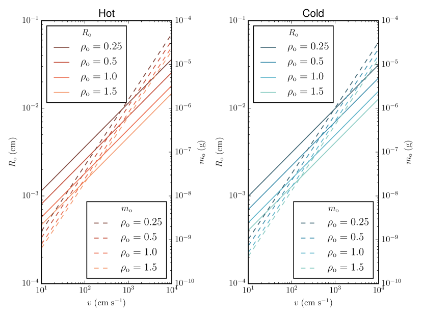
Figure 2: Expected size and mass of an organism for a given windspeed determined using the analytical model. The line colour denotes the density of the organism including the cavity. Solid lines denote the radius, $R_{\mathrm{o}}$, required for the sinking rate to match the upward windspeed. The dashed lines denote the corresponding mass, $m_{\mathrm{o}}$. Hot denotes the hotter, lower AHZ ($395~{}\mathrm{K}$) and cold denotes the colder, higher AHZ ($258~{}\mathrm{K}$), which use corresponding values for $\nu$ and $\rho_{\mathrm{gas}}$ ($0.1~{}\mathrm{cm^{2}~{}s^{-1}}$ and $1.2~{}\mathrm{g~{}cm^{-3}}$, or $0.2~{}\mathrm{cm^{2}~{}s^{-1}}$ and $0.4~{}\mathrm{g~{}cm^{-3}}$, respectively).

3.2 Numerical Model Estimates

Our control model experiment has a convective windspeed of $100~{}\mathrm{cm~{}s^{-1}}$, a timestep of six hours, a initial population of 100 organism with an approximate mass of $10^{-9}~{}\mathrm{g}$ distributed randomly (with a uniform distribution) across the AHZ. Each organism is initialized with random properties. We run an ensemble of 20 simulations, each for 100 Earth years.

We test each simulations for steady state conditions by looking at the stationarity of the total number of organisms; a trend or changing variance would indicate that the population was still undergoing changes and had not yet settled to a viable strategy. To achieve this we use an augmented Dickey-Fuller (henceforth ADF) test (Said & Dickey 1984) on the last 75 years of population data and found that all runs had reached steady state to a very high significance ($p<0.01$). We present results that represent the mean model state from the last Earth year of each experiment.

Figure 3 shows that organisms are approximately evenly spread throughout the AHZ with a small skew towards to the top. An approximate even distribution suggest that the organism have found a mass/size strategy to support a stable population. In general this strategy is found within a few years. The age distribution of the organisms follow the expected half-life distribution well, with the exception of a large number of very young organisms. These small organisms are also visible in the mass, skin width and size distributions. We find this population is a persistent feature of our experiments, but individuals have a short residence time as they are rapidly convected out of the AHZ. The population is an artifact of our reproduction scheme: individually they are unviable but are frequently produced as they only require a small amount of mass. The densities are evenly spread across the allowed range with a small skew to higher densities, suggesting that there is most likely no significant effect on the dynamical behaviour of the organisms. Densities are forced within the range $0.5~{}\mathrm{g~{}cm^{-3}}<\rho_{\mathrm{o}}<1.5~{}\mathrm{g~{}cm^{-3}}$, which accounts for the small excesses at either end of the distribution. Aside from the population of small, short-lived organisms, the mass distribution peaks at around $2\times 10^{-8}~{}\mathrm{g}$, with most organisms being between $10^{-9}$ and $10^{-7}~{}\mathrm{g}$, which is consistent with the analytical model. Organisms within this range are relatively stable in the convection, with residence times of 30 days or more.

We find that the growth strategy favoured by the organisms in the control calculation is skewed towards lower values of $G$, i.e. particles that are more solid. As discussed above for the analytical calculations, the effect of the growth strategy on the organism’s size or effective density goes approximately with the cube of $G$. Thus values of $G<0.8$ have very little effect on the dynamical behaviour of the organism, which we see in the distribution. The distribution of skin widths and size is as expected with the peak value for the skin width between $0.3$ and $3\times 10^{-3}~{}\mathrm{cm}$, consistent with the analytical model.

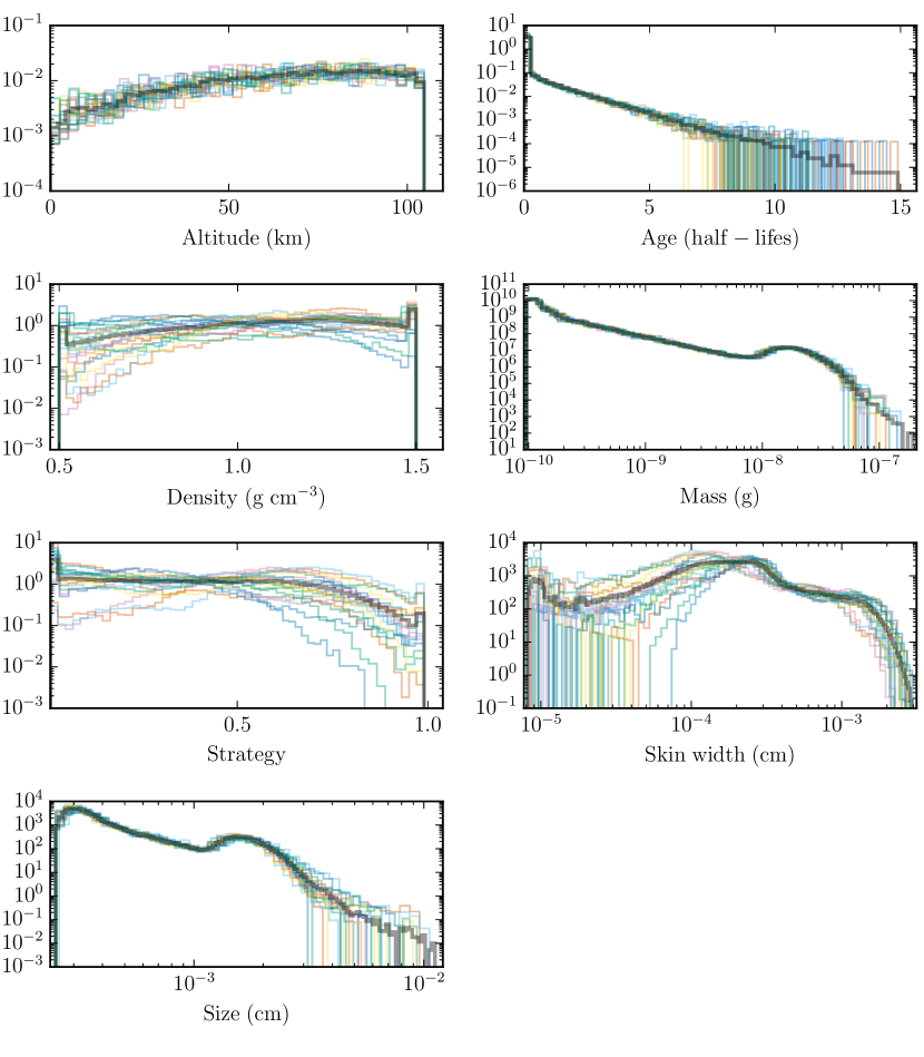
Figure 3: Normalized frequency distributions of organisms in the AHZ as a function of altitude, age (as half-lives), density, mass, growth strategy, skin width, and size. The dark lines denote the average of the ensemble of the 20 individual model run shown by coloured lines. The frequency distribution is normalized such that its integrates to unity between the lowest and highest values.

3.3 Sensitivity Runs

Table 1: Sensitivity Runs

Description	$m_{\mathrm{input}}~{}(\mathrm{g})$	$B$	$\tau~{}(\mathrm{hrs})$	$v_{\mathrm{conv.}}~{}(\mathrm{cm~{}s^{-1}})$	$T_{1/2}~{}(\mathrm{days})$
Control run	$10^{-9}$	1	6	100	30
High windspeeds	$10^{-8}$	1	2	1000	30
Radiative windspeeds	$10^{-13}$	1	6	0.01	30
Population increase	$10^{-9}$	3	6	100	30
Initial input mass	$2\times 10^{-9}$	1	6	100	30
Short half-life	$10^{-9}$	1	6	100	15
Long half-life	$10^{-9}$	1	6	100	60

Note. — Initial conditions for each set of sensitivity runs. Shown is the mean initial organism mass $m_{\mathrm{input}}$, the approximate biomass factor $B$ relative to the control run, the timestep in Earth hours $\tau$, the windspeed $v_{\mathrm{conv.}}$, and the half-life of the organism $T_{1/2}$.

We run a small set of sensitivity runs to test our prior model assumptions; for each sensitivity experiment we run a ensemble of 10 replicates. Table 1 summarizes the We use the ADF to ensure that all resulting populations were stable and sustainable. We find that our results are not significantly sensitive to changes in the initial conditions for the organisms (e.g. amount of available biomass) and these results are not discussed further.

We run the models with vertical velocities of $1000~{}\mathrm{cm~{}s^{-1}}$ and $0.01~{}\mathrm{cm~{}s^{-1}}$. The slower of these velocities is intended to replicate windspeeds in the radiative zone. Most models put the radiative-convective boundary somewhere above the AHZ, but it is possible for it to be below the AHZ or even inside it. Changing the wind speed will affect the range of masses that could be sustained in the AHZ: generally, slower convection supports the evolution of lighter organisms and higher convection supports the evolution of heavier organisms.

There are two implications of changing the vertical velocity that we consider when choosing the lower and upper values. First, varying the windspeed will change the distribution of organism sizes and masses that can sustain a population. To address this we also change the range of masses that are allowed within the model based on the analytical model results described above. Second, changing the vertical velocity changes the distance over which organisms can move during one timestep. We have addressed this by co-adjusting the timestep so that the Courant Friedrichs Lewy criterion is met (Courant et al. 1928). We find that our results are not significantly affected by changing the model timestep.

Figure 4 and Figure 5 shows that the organism population distributions corresponding to vertical velocities of $1000~{}\mathrm{cm~{}s^{-1}}$ and $0.01~{}\mathrm{cm~{}s^{-1}}$, respectively, are different to those from the control run. We find that skin widths peak at around $5\times 10^{-4}~{}\mathrm{cm}$ and $3\times 10^{-3}~{}\mathrm{cm}$ with sizes showing two peaks at $7.5\times 10^{-4}~{}\mathrm{cm}$ and $8\times 10^{-3}~{}\mathrm{cm}$. Thus in most cases organisms have small cavities, which is also reflected in the strategy graph. Masses drop off steadily from $10^{-9}~{}\mathrm{g}$ to a second peak at $10^{-6}~{}\mathrm{g}$. Here the analytical calculations have somewhat overestimated the required mass to sustain a population. Age and altitude graphs are consistent with the control run.

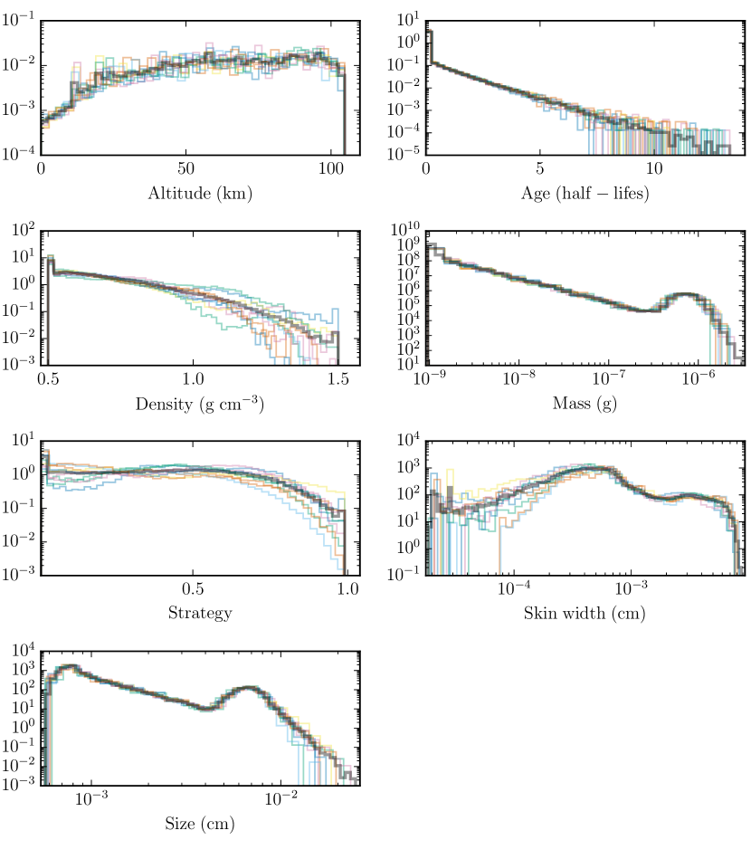
Figure 4: As Figure 3 but using a convective velocity of $1000~{}\mathrm{cm~{}s^{-1}}$.

For the radiative experiment, the organism distributions are generally similar to those of the control experiment. This is a skew in the vertical distributon of the organisms, where there are approximately twice as many organisms at the bottom of the atmosphere when compared with the top. The age distribution is close to a perfect half-life distribution. This non-convective environment also appears to support a slightly wider range of growth strategies. Unlike the control experiment, the non-convective environment cannot support the highest masses with the distribution falling off near-monotonically in log-space. This is consistent with our analytic model that shows that for every tenfold decrease in windspeed organisms should decrease in mass by a factor of $10^{3/2}$. The expected mass of approximately $10^{-14}~{}\mathrm{g}$ is comparable to the mass of a terrestrial virus (Johnson et al. 2006). Terrestrial microbes are a factor of ${\sim}100$ too massive to be supported by this environment. This environment could be considered as habitable if life could be described by something much smaller than a terrestrial microbe.

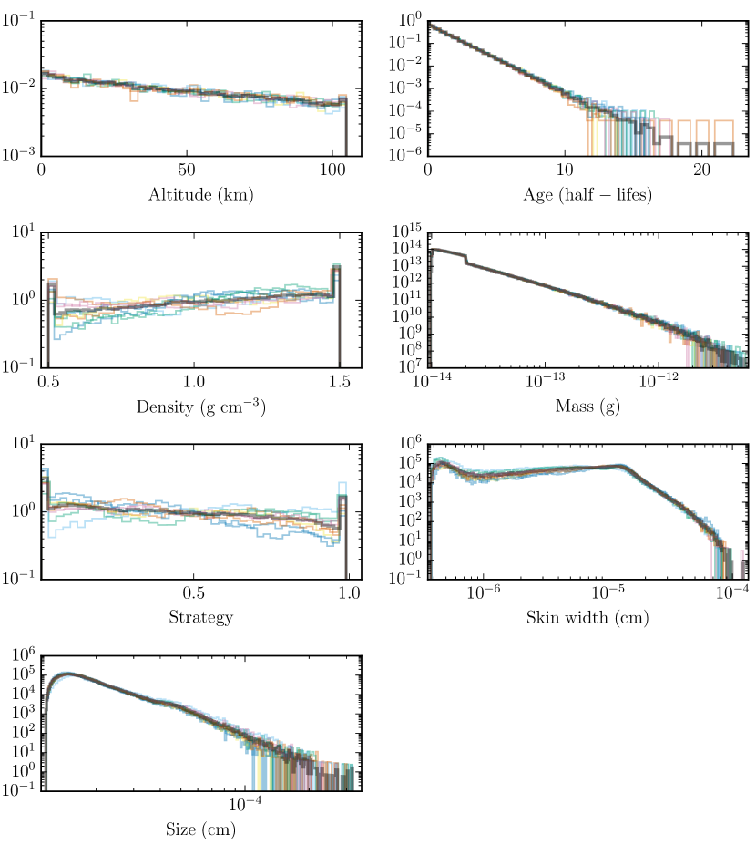
Figure 5: As Figure 3 but using a radiative vertical velocity of $0.01~{}\mathrm{cm~{}s^{-1}}$.

The half-life of organisms will impact the ability of the AHZ to sustain life. For example, shorter organism half-lives mean greater turnover of biomass and a reduced emphasis on the atmospheric transport in determining observed variations. To address this we used a half-life that was half and double that of the 30-day control run value. For organisms with a 15-day half-life there is an excess of very young organisms compared with old organisms, which is due to a higher turnover of biomass that increases birth rates. Other distributions are not significantly different from the control case.

4 Discussion

Here, we put our model results into a wider context. We also discuss briefly the associated implications for habitability.

4.1 Cool Brown Dwarf Spatial Frequency and Galactic Significance

There are only tens of known cool brown dwarfs of which WISE 0855-0714 is the coolest. These objects are inherently faint and consequently are difficult to detect unless they are nearby. To understand how common AHZs might be, we extrapolate from the number of known Y dwarf objects (though the results are likely applicable to other types of bodies).

To estimate the frequency of these cool brown dwarfs, we determine spatial densities based on the distances of known objects, following Kirkpatrick et al. (2012). For objects that are uniformly distributed in space, with some objects yet to be discovered, we perform a $V/V_{\mathrm{max}}$ test to assess the completeness of a sample. First, we calculate the interior volume $V_{i}$ of each real object, i.e. the spherical volume centred on Earth, with radius $d_{i}$, where $d_{i}$ is the distance to object $i$. The sample is assumed to be complete out to some distance $d_{\mathrm{max}}$. Within the corresponding interior volume, $V_{\mathrm{max}}$, the mean value of $V_{i}/V_{\mathrm{max}}{}$ should be 0.5. Using the value of $d_{\mathrm{max}}$, we can estimate the spatial density of the objects by dividing the number of objects closer than $d_{\mathrm{max}}$ by $V_{\mathrm{max}}$. Here, we calculate $d_{\mathrm{max}}$ for each spectral type, rather than define a value of $d_{\mathrm{max}}$ and assess the completeness (Kirkpatrick et al. 2012). (Naturally, we reject objects with $V_{i}/V_{\mathrm{max}}{}>1$. In this case we remove the objects and recalculate $V_{\mathrm{max}}$ until all objects have $V_{i}/V_{\mathrm{max}}{}>1$.)

We analyzed brown dwarfs of spectral type Y0 or later with published parallaxes, using the data from Tinney et al. (2014) and references therein. Where there is more than one published parallax, we take a mean weighted by the inverse of the square of the uncertainties. We group objects into two spectral type categories: spectral types $\mathrm{Y}0-0.5$ and $\geq\mathrm{Y}1$.

For the $\mathrm{Y}0-0.5$ category we include 9 objects and reject 4. We find $d_{\mathrm{max}}{}=9.6~{}\mathrm{pc}$, $V_{\mathrm{max}}{}=3.6\times 10^{3}~{}\mathrm{pc^{3}}$ and a spatial density of $\sim 2.5\times 10^{-3}~{}\mathrm{pc^{-3}}$. For the $\geq\mathrm{Y}1$ objects, we include 3 objects and reject 1. Here we find $d_{\mathrm{max}}{}=10.85$, $V_{\mathrm{max}}{}=5.4\times 10^{3}~{}\mathrm{pc^{3}}$ and a spatial density of $\sim 0.6\times 10^{-3}~{}\mathrm{pc^{-3}}$.

Assuming the Milky Way is a disk with a diameter of $4\times 10^{4}~{}\mathrm{pc}$ and a thickness of $600~{}\mathrm{pc}$ (corresponding to a volume of $\simeq$750$\times 10^{9}~{}\mathrm{pc^{3}}$), we can project these numbers on to the galaxy as a whole. These calculations produce very approximate numbers of $2\times 10^{9}$ objects with spectral type $\mathrm{Y}0-0.5$ and $0.5\times 10^{9}$ objects with spectral type $\geq\mathrm{Y}1$ in the galaxy. Further, we expect that there should be around 10 $\mathrm{Y}0-0.5$ dwarfs and 2 $\geq\mathrm{Y}1$ dwarfs within 10 pc of Earth.

Clearly these samples are highly incomplete so we consider this a conservative estimate. Brown dwarf cool as they age on timescales of billions of years (Baraffe et al. 2003). Hotter objects will eventually develop an AHZ, while for cooler objects the AHZ will descend in the atmosphere and will contract as the effective temperature falls and the lapse rate grows. As the AHZ descends the associated pressure will increase so that the nature of the organisms as we describe them here will undoubtedly change.

4.2 Implications for Habitability

Estimating the total potential biomass achievable in an aerial biosphere of a brown dwarf for which we have very limited knowledge of the elemental composition of the atmosphere, let alone the nutritional requirements of a hypothetical biota, cannot be done with accuracy. We still have much to learn about how nutrient limitation and co-limitation influences the distribution of biomass on Earth. However, from a more general point of view, we would expect that the upper limit of biomass theoretically achievable in a brown dwarf atmosphere to be determined by limitation of specific nutrients. Once more data are available on the atmospheric composition of very cool brown dwarf atmospheres it may even be possible to predict which elements would limit a potential biota in these environments. We are not aware of any modelling studies predicting the presence of phosphorus in significant quantities.

The implications of the AHZ concept for habitability in the galaxy are significant. In the most simplistic view there are, conservatively, billions of cool brown dwarfs in the galaxy and hundreds within a few tens of parsec of the Earth. Some of these will be targets for characterisation for next-generation telescopes in less than a decade, although their inherent faintness makes them difficult to find in surveys.

When searching for habitable environments, we naturally take an Earth-centric focus on terrestrial planets that receive their energy from the host star. Thermal spectra of W0855-0714 shows features consistent with atmospheric water vapour and clouds (Skemer et al. 2016), suggesting that self-heating is sufficient to produce an atmosphere with liquid water at habitable temperatures. This observation is not limited to application to brown dwarfs; Jupiter receives approximately as much heating from the Sun as from its core, as does Saturn. Gas giants in other stellar systems could also potentially support similar biomes. Our work provides further evidence for the habitability of planets such as Venus that have an uninhabitable surface. Whilst the dynamics of Venus’ atmosphere will likely be very different to that of a cool brown dwarf or gas giant, it seems likely that with some adjustment of the properties one could model an organism that could sustain a population in the Venusian AHZ indefinitely. Thus we support the idea that the inner edge of the circumstellar habitable zone is not a hard limit on habitability. Detecting this aerial biosphere with current and next-generation telescopes will depend on the range and resolution of the spectrally-resolving instruments, and also the range and magnitude of byproduct gases that the organisms produce.

4.3 Reflections on our Model Organism

We described organisms as individual frictionless hollow spheres with a permeable skin. Organisms that successively evolved within the prescribed physical environment of the AHZ eventually shaped the final cohort that were characterized by their radius and skin thickness. While our organism model does exist in nature, e.g., pollen spore with air sacs, we did not impose any further constraint that could impact their atmospheric lifetime in the AHZ.

We did not consider the coalescence of similar organisms or deposition onto existing airborne particles. Earth bacteria can occur as agglomerations of cells or attach themselves to airborne particulate matter, such as pollen, or aqueous-phase aerosol (Jones & Harrison 2004). In our simple approach, we can consider an organism as a single entity or an agglomeration of many entities. Heavier organisms sink in the atmosphere at greater speeds. Organisms made of lots of individual entities could employ an additional survival strategy: organisms could attach to each other or to atmospheric particulates as temperature decreases (as they ascend), and disperse as temperature increases (as they descend), allowing them to self-correct to find the centre of the AHZ. This strategy is similar to that proposed by Sagan & Salpeter (1976), where organisms increase in mass and split into low-mass daughter cells as they sink to the lower parts of the AHZ.

We also did not consider cryogenic freezing of organisms above the top of the AHZ. It is conceivable that an organism could pass through the upper boundary of the AHZ, spend some time in statis and subsequently sink back into the AHZ, whereupon it would thaw and reactivate. We anticipate that low-mass or low-density organisms would have greater survivability in this scenario.

Surface roughness is another parameter that organisms could use to adapt to their environment. A rough surface would increase the drag properties of the organism, resulting in slower movement that deviates significantly from Stoke’s formula (Md et al. 2015). Recent empirical evidence also suggests that if a microorganism has the ability to maintain a charge it could substantially decrease its drag and speed up its trajectory (Md et al. 2015). If the charge could be manipulated it could be used to stabilize the altitude of organisms.

In nature, there a number of examples where animals manipulate their body drag through water. Fish can alter the drag between their skin and medium by altering their body smoothness by excreting high-molecular weight polymer compounds and surfactants (Daniel 1981) or in the case of sharks by altering their body geometry (Dean & Bhushan 2010). Studies have also proposed that seals and penguins actively use bubble-mediated drag reduction, required to launch themselves out of water (Davenport et al. 2011).

While our model of an organism is rudimentary there do exist in nature a number of examples in which animals control their movement in a laminar flow. Therefore it is possible that our microorganisms could have evolved to stabilize their movement without the need for necessarily changing their physical dimensions.

5 Conclusions

We used a simple organism lifecycle model to explore the viability of an atmospheric habitable zone (AHZ), with temperatures that could support Earth-centric life. The AHZ sits above some uninhabitable environment, such as an uninhabitable surface (e.g. as on Venus) or a hot dense atmosphere (e.g. the lower atmosphere of a brown dwarf or gas giant). We based our organism model on previous work that explored whether the Jovian atmosphere could support life. We illustrated this idea using a cool Y brown dwarf, for example object W0855-0714.

Our atmospheric model assumed availability of liquid water that is necessary to support the biochemistry associated with life. There exist valid counter arguments for the presence of liquid water in the AHZ of a cool brown dwarf (e.g., changes in metallicity may affect partial pressure of water, although metallicity has to change by orders of magnitude to affect H₂O (Helling et al. 2008)), which may suggest that our model is valid only for a small subset of available cool Y dwarfs (and a range of gas giants). The formation history of brown dwarfs result in a wide range of atmospheric chemical composition environments, e.g. Madhusudhan et al. (2016). In the authors’ view the most compelling argument for the presence of liquid water is the observed thermal spectra of WISE 0855-0714 that showed evidence of atmospheric water and clouds (Skemer et al. 2016). Based on our understanding of Earth’s atmosphere, water clouds cannot exist without the presence of liquid water. We also assumed a constant upward vertical velocity through the AHZ and model organisms that float in the convective updrafts. Our modelled organisms can adapt to their atmospheric environment by adopting different growth strategies that maximize their chance of survival and producing progeny. We found that the organism growth strategy is most sensitive to the magnitude of the atmospheric convection. Stronger convective winds support the evolution of more massive organisms with higher gravitational sinking rates, counteracting the upward force, while weaker convective winds results in organisms that need less mass to overcome the upward convective force. For a purely radiative environment we found that the successful organisms will have a mass that is ten times smaller than terrestrial microbes, thereby putting some dynamical constraints on the dimensions of life that the AHZ can support.

We explored the galactic implications of our results by considering the likely number of Y brown dwarfs in the galaxy, based on the number we know. We calculate that of order $10^{9}$ of these objects reside in the Milky Way with a few tens within ten parsecs of Earth. Some of these close objects will be visible to large telescopes in the next decade. Our work has focused on brown dwarfs but it also has implications for exploring life on gas giants in the solar system and exoplanets, which have uninhabitable surfaces. Our calculations suggest a significant upward revision of the volume of habitable space in the galaxy.

References

- Allard et al. (2012) Allard, F., Homeier, D., & Freytag, B. 2012, Philosophical Transactions of the Royal Society A: Mathematical, Physical and Engineering Sciences, 370, 2765
- Baraffe et al. (2003) Baraffe, I., Chabrier, G., Barman, T. S., Allard, F., & Hauschildt, P. H. 2003, Astronomy and Astrophysics, 402, 701
- Beamín et al. (2014) Beamín, J. C., Ivanov, V. D., Bayo, A., et al. 2014, Astronomy and Astrophysics, 570, L8
- Bowers et al. (2012) Bowers, R. M., McCubbin, I. B., Hallar, A. G., & Fierer, N. 2012, Atmospheric Environment, 50, 41
- Cockell (1999) Cockell, C. S. 1999, Planetary and Space Science, 47, 1487
- Côté et al. (2008) Côté, V., Kos, G., Mortazavi, R., & Ariya, P. a. 2008, Science of the Total Environment, 390, 530
- Courant et al. (1928) Courant, R., Friedrichs, K., & Lewy, H. 1928, Mathematische Annalen, 100, 32
- Cushing et al. (2004) Cushing, M. C., Rayner, J. T., & Vacca, W. D. 2004, The Astrophysical Journal, 25
- Cushing et al. (2006) Cushing, M. C., Roellig, T. L., Marley, M. S., et al. 2006, The Astrophysical Journal, arXiv:0605639
- Cushing et al. (2007) Cushing, M. C., Marley, M. S., Saumon, D., et al. 2007, The Astrophysical Journal, 44
- Cushing et al. (2011) Cushing, M. C., Kirkpatrick, J. D., Gelino, C. R., et al. 2011, The Astrophysical Journal, 743, 50
- Daniel (1981) Daniel, T. L. 1981, Biological Bulletin, 160, 376
- Dartnell et al. (2015) Dartnell, L. R., Nordheim, T. A., Patel, M. R., et al. 2015, Icarus, 257, 396
- Davenport et al. (2011) Davenport, J., Hughes, R. N., Shorten, M., & Larsen, P. S. 2011, Mar. Ecol. Prog. Ser.
- Dean & Bhushan (2010) Dean, B., & Bhushan, B. 2010, Philosophical Transactions of the Royal Society of London A: Mathematical, Physical and Engineering Sciences, 368, 4775
- Faherty et al. (2014) Faherty, J. K., Tinney, C. G., Skemer, A., & Monson, A. J. 2014, The Astrophysical Journal, 793, L16
- Franks (2002) Franks, P. J. S. 2002, Journal of Oceanography, 58, 379
- Fuzzi et al. (1997) Fuzzi, S., Mandrioli, P., & Perfetto, A. 1997, Atmospheric Environment, 31, 287
- Gandolfi et al. (2013) Gandolfi, I., Bertolini, V., Ambrosini, R., Bestetti, G., & Franzetti, A. 2013, Applied Microbiology and Biotechnology, 97, 4727
- Gilichinsky et al. (2008) Gilichinsky, D., Vishnivetskaya, T., Petrova, M., et al. 2008, Bacteria in Permafrost (Berlin, Heidelberg: Springer Berlin Heidelberg), 83–102
- Helling & Casewell (2014) Helling, C., & Casewell, S. 2014, The Astronomy and Astrophysics Review, 22, 80
- Helling & Fomins (2013) Helling, C., & Fomins, A. 2013, Philosophical Transactions of the Royal Society of London A: Mathematical, Physical and Engineering Sciences, 371, http://rsta.royalsocietypublishing.org/content/371/1994/20110581.full.pdf
- Helling et al. (2008) Helling, C., Ackerman, A., Allard, F., et al. 2008, Monthly Notices of the Royal Astronomical Society, 391, 1854
- Johnson et al. (2006) Johnson, L., Gupta, A. K., Ghafoor, A., Akin, D., & Bashir, R. 2006, Sensors and Actuators B: Chemical, 115, 189
- Jones & Harrison (2004) Jones, A. M., & Harrison, R. M. 2004, Science of The Total Environment, 326, 151
- Kasting et al. (1993) Kasting, J. F., Whitmire, D. P., & Reynolds, R. T. 1993, Icarus, 101, 108
- Kirkpatrick et al. (2012) Kirkpatrick, J. D., Gelino, C. R., Cushing, M. C., et al. 2012, The Astrophysical Journal, 753, 156
- Koop et al. (2000) Koop, T., Luo, B., Tsias, A., & Peter, T. 2000, Nature, 406, 611
- Kopytova et al. (2014) Kopytova, T. G., Crossfield, I. J. M., Deacon, N. R., et al. 2014, The Astrophysical Journal, 797, 3
- Lawson & Gettelman (2014) Lawson, R. P., & Gettelman, A. 2014, Proceedings of the National Academy of Sciences, 111, 18156
- Lighthart (1997) Lighthart, B. 1997, FEMS Microbiology Ecology, 23, 263
- Lighthart & Shaffer (1995) Lighthart, B., & Shaffer, B. T. 1995, Aerobiologia, 11, 19
- Loewe et al. (2016) Loewe, K., Ekman, A. M. L., Paukert, M., et al. 2016, Atmospheric Chemistry and Physics Discussions, 2016, 1
- Luhman (2014) Luhman, K. L. 2014, The Astrophysical Journal, 786, L18
- Madhusudhan et al. (2016) Madhusudhan, N., Apai, D., & Gandhi, S. 2016, Submitted to ApJ
- McKay (2014) McKay, C. P. 2014, Proceedings of the National Academy of Sciences, 111, 12628
- Md et al. (2015) Md, A., Kabir, R., Inoue, S., et al. 2015, Polymer Journal
- Morley et al. (2014a) Morley, C. V., Marley, M. S., Fortney, J. J., & Lupu, R. 2014a, The Astrophysical Journal, 789, L14
- Morley et al. (2014b) Morley, C. V., Marley, M. S., Fortney, J. J., et al. 2014b, The Astrophysical Journal, 787, 78
- Morrison et al. (2012) Morrison, H., de Boer, G., Feingold, G., et al. 2012, Nature Geosci, 5, 11
- Muñoz Caro et al. (2002) Muñoz Caro, G. M., Meierhenrich, U. J., Schutte, W. A., et al. 2002, Nature, 416, 403
- Rogers & Yau (1995) Rogers, R. R., & Yau, M. K. 1995, A short course in cloud physics (Elsevier), iSBC 0-7506-3215-1
- Sagan & Salpeter (1976) Sagan, C., & Salpeter, E. E. 1976, The Astrophysical Journal Supplement Series, 32, 737
- Said & Dickey (1984) Said, S. E., & Dickey, D. A. 1984, Biometrika, 71, 599
- Sattler et al. (2001) Sattler, B., Puxbaum, H., & Psenner, R. 2001, Geophysical Research Letters, 28, 239
- Schulze-Makuch et al. (2004) Schulze-Makuch, D., Grinspoon, D. H., Abbas, O., Irwin, L. N., & Bullock, M. a. 2004, Astrobiology, 4, 11
- Showman & Kaspi (2013) Showman, A. P., & Kaspi, Y. 2013, The Astrophysical Journal, 776, 85
- Skemer et al. (2016) Skemer, A. J., Morley, C. V., Allers, K. N., et al. 2016, The Astrophysical Journal, 826, L17
- Stark et al. (2014) Stark, C. R., Helling, C., Diver, D. A., & Rimmer, P. B. 2014, International Journal of Astrobiology, 13, 165
- Tinney et al. (2014) Tinney, C. G., Faherty, J. K., Kirkpatrick, J. D., et al. 2014, The Astrophysical Journal, 796, 39
- Tsuji (2005) Tsuji, T. 2005, The Astrophysical Journal, 621, 1033
- Witte et al. (2011) Witte, S., Helling, C., Barman, T., Heidrich, N., & Hauschildt, P. H. 2011, Astronomy and Astrophysics, 529, A44
- Wölk & Strey (2001) Wölk, J., & Strey, R. 2001, The Journal of Physical Chemistry B, 105, 11683
- Womack et al. (2010) Womack, A. M., Bohannan, B. J. M., & Green, J. L. 2010, Philosophical transactions of the Royal Society of London. Series B, Biological sciences, 365, 3645