DrivingStyles: A mobile platform for driving styles and fuel consumption characterization

Abstract

Intelligent Transportation Systems (ITS) rely on connected vehicle applications to address real-world problems. Research is currently being conducted to support safety, mobility and environmental applications. This paper presents the DrivingStyles architecture, which adopts data mining techniques and neural networks to analyze and generate a classification of driving styles and fuel consumption based on driver characterization. In particular, we have implemented an algorithm that is able to characterize the degree of aggressiveness of each driver. We have also developed a methodology to calculate, in real-time, the consumption and environmental impact of spark ignition and diesel vehicles from a set of variables obtained from the vehicle’s Electronic Control Unit (ECU). In this paper, we demonstrate the impact of the driving style on fuel consumption, as well as its correlation with the greenhouse gas emissions generated by each vehicle. Overall, our platform is able to assist drivers in correcting their bad driving habits, while offering helpful tips to improve fuel economy and driving safety.

1 Introduction

Intelligent transportation systems (ITS) introduce advanced applications aimed at providing innovative services, offering traffic management and enabling users to be better informed, including support for safety, mobility, and environmental applications. In parallel to ITS, mobile devices have experienced technological breakthroughs in recent years, evolving towards high performance terminals with multi-core microprocessors. The smartphone is a clear representative outcome of this trend.

In addition, the On Board Diagnostics (OBD-II) [1] standard, available since 1994, has recently become an enabling technology for in-vehicle applications due to the availability of Bluetooth OBD-II connectors. These connectors enable a transparent connectivity between the mobile device and the vehicle’s Electronic Control Unit (ECU).

When combining high performance smartphones with OBD-II connectivity, new and exciting research challenges emerge, promoting the symbiosis between vehicles and mobile devices, and thereby achieving novel intelligent systems. DrivingStyles implements a solution based on neural networks, which is capable of characterizing the driving style of each user [2], as well as the fuel consumption [3]. In order to achieve this functionality, the data is obtained from the ECU via the OBD-II Bluetooth interface, including the speed, acceleration, revolutions per minute of the engine, mass flow sensor (MAF), manifold absolute pressure (MAP), and intake air temperature (AIT). Currently, this information can be collected and used in applications aimed at improving road safety and promoting eco-driving, thus reducing fuel consumption and greenhouse gas emissions. Specifically we find that, by shifting towards a more efficient driving style, users can save up to 20% of fuel while improving driving safety, thereby reducing greenhouse gases as we detail later on.

This paper is organized as follows: in the next section we present some related works. Section 3 introduces the DrivingStyles architecture (both the Android and the server interface). Models for fuel consumption and $CO_{2}$ emissions, are described in more detail in section 4. The tuning of the neural network, along with the obtained results, are presented in sections 5 and 6, respectively. Finally, section 7 presents the conclusion of our work.

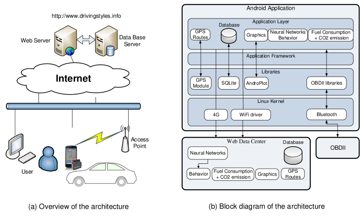
Figure 1: System Architecture of DrivingStyles.

2 Related Work

Technological advancements in the field of mobile telephony are making smartphones very powerful. This high computing power opens new and attractive opportunities for research. When coupled with the eco-driving concept, it has gained great significance in recent years [4]. An example is the prototype of an onboard unit developed by Hernandez et al. [5]. These driving techniques save fuel consumption, regardless of the technology used inside the vehicle. One of the main problems of eco-driving systems is identifying the factors that affect energy consumption. Ericsson [6] suggests that, in order to save fuel, sudden changes in acceleration and high speed driving should be avoided. Johansson et al. [7] suggest maintaining low levels of deceleration, minimizing the use of the first and second gears, and putting every effort into using the 5th and 6th gears, while avoiding continuous gear changes.

There are several proposals that analyze which variables affect fuel consumption. Kuhler [8] introduced a set of ten variables that are used in laboratories for fuel consumption and vehicle emissions analysis. Other authors such as Andr [9] improve these results by increasing and replacing some of the parameters. In previous works such as Leung [10] and COPERT III [11], different tools were developed to enable real-time collection of engine and vehicle parameters from the OBD connector.

Several commercial OBD-II scanner tools are available that can read and record these sensor values. Apart from such scanners, remote diagnostic systems such as GM’s OnStar, BMW’s Connected Drive, and Lexus Link are capable of monitoring engine parameters from a remote location. Car manufacturers used eco-monitoring to reflect the instant, historical, and time-elapsed fuel economy, and is used in the car through on-board trip computers [12]. Our solution differs from all the previous ones by providing a real-time analysis of the driving style of each user in the scope of eco-driving behavior, and based on neural network techniques. By calculating the consumption and greenhouse gas emissions generated by both types of engines (spark ignition, and diesel vehicles), we are able to closely relate both results, detailing the fuel savings achieved by soft driving patterns when compared to aggressive ones.

3 DrivingStyles Architecture

Our proposed architecture applies data mining techniques to generate a classification of the driving styles of users based on the analysis of their mobility traces. Such classification is generated taking into consideration the characteristics of each route, such as whether it is urban, suburban, or a highway, and it is then correlated with the fuel consumption and emissions of each driver.

To achieve the overall objective, our system comprises four elements:

1. An application for Android, based smartphones. Using an OBD-II Bluetooth interface, the application collects control information (by default every second, but it is configurable by the user) such as speed, acceleration, engine revolutions per minute, throttle position, and the vehicle’s geographic position. In addition, we also obtain via OBD-II the mass flow sensor (MAF), the manifold absolute pressure (MAP), and the intake air temperature (AIT) that are used in the calculation of fuel consumption. After gathering the information, the user can upload the collected data to the remote data center for analysis.

2. A data center offering a web interface to collect large data sets sent by different users concurrently, and to graphically display a summary of the most relevant results, like driving styles and route characterization of each route sent. Our solution is based on open source software tools such as Apache, PHP and Joomla.

3. A neural network, which has been trained using the most representative route traces in order to correctly identify, for each path segment, the driving style of the driver, as well as the segment profile: urban, suburban or highway. We use the backpropagation algorithm [13], which has proven to provide good results in classification problems such as the one associated to this project.

4. Integration of the tuned neural networks both within the mobile device itself, and in the data-center platform. The goal is to use neural networks to dynamically and automatically analyze user data, reporting to the drivers in real time and allowing them to find out their driver profile, thus promoting a less aggressive and more ecological driving.

The block diagram of the DrivingStyles architecture is shown in figure 1b. This consists of three blocks: the mobile application on a Android device, the data center platform, and an On Board Diagnostics (OBD-II) device.

The basic layer in the Android device is the Linux kernel, which contains all the essential hardware drivers to interact with the OBD-II device via Bluetooth. The top layer includes both Android’s native libraries and our own libraries. Specifically, we developed the OBD-II communications module, along with the libraries for graphical data representation, at this layer. The next level up is the Application Framework; this layer manages the basic functions of the mobile device, and the communications with the developed libraries.

Finally, at the application layer, we developed the different modules of the DrivingStyles architecture, such as the fuel consumption and $CO_{2}$ emissions estimators, the neural networks behavior, GPS routes, and graphics. Also, the application provides real-time feedback from the device to the user such that, when it detects high levels of aggressiveness (above a certain threshold), the device automatically generates an acoustic signal to alert the driver.

3.1 DrivingStyles Android Interface

The first step for a user is to register at http://www.drivingstyles.info, and to download the free Android application. After installing the Android application in the mobile device, and after connecting to the Bluetooth ELM327 interface inside the car (this connector is mandatory on all vehicles since 2001), the data acquisition process will start (see figure 1a).

The Android application is a key element of our system, proving connectivity to the vehicle and to the DrivingStyles web platform. Currently, it can be downloaded for free from the DrivingStyles website, or from Google Play .

Once the mobile application is installed and configured, the user must pair the mobile device with the ELM327 (OBD-II Bluetooth device) to start getting data. The data obtained from the different variables such as acceleration, engine revolutions per minute (RPM), speed, mass flow sensor (MAF), manifold absolute pressure (MAP), and intake air temperature (IAT) are analyzed by the application, showing users the characteristics related to their driving, fuel consumption, and $CO_{2}$ emissions.

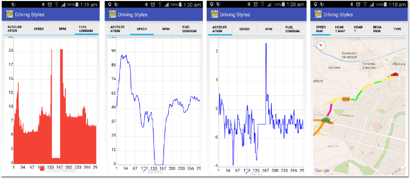
Figure 2: Snapshots of the fuel consumption, speed, acceleration parameters, and map module for the Android application.

In order to adjust the application functionality, it offers several configuration options, i.e., User creation, Connection options, GPS Activation, Sensor sampling, and type of fuel definition. Once configured, our application captures data sent by the OBD-II and the GPS interfaces, as well as the phone’s accelerometer showing the monitored sensors, and performing several monitoring actions in real time without affecting the data captured. Figure 2, shows some snapshots of our DrivingStyles application.

In addition, routes traces can also be sent to the website data center for further analysis. This module can be accessed either from the historic stored routes, or immediately after stopping the data capture. The information screen displays the header information of the selected route, such as: (i) date of the captured data, (ii) start time, (iii) finish time, (iv) maximum speed, and (v) fuel consumption. The URL of the DrivingStyles web interface is http://www.drivingstyles.info.

3.2 DrivingStyles Server Interface

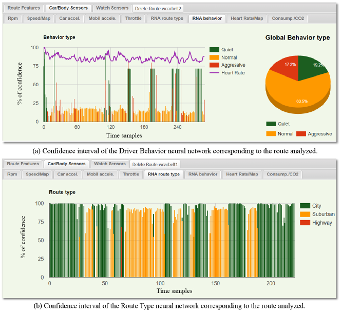
Figure 3: Snapshots of driver behavior and route type corresponding to the data center web.

The second main component of our architecture corresponds to the data center and its web interface. To implement this component, we have selected open source software such as Apache HTTP, and Joomla as the content management system (CMS). We have used a CMS, combined with the use of a resource wrapper, which detachs our system from the presentation layer, thus focusing on the driving styles characterization problem. This module can be found in http://www.drivingstyles.info.

Basically the server receives data sent from the Android application of each user, and it provides functionality to work with User, Routes, and Statistics.

Once the user is logged in, he is asked to record a number of important data, especially for future data mining studies. The most relevant items are sex, age, and other details concerning the vehicle used: car manufacturer, model, fuel type, and the theoretical 0-100 acceleration level (important to normalize the user behavior in our study).

In the Routes’ section, users can access all the routes they have uploaded. When selecting car/body sensors, the system displays nine graphs for the different sensors obtained from the OBD-II (direct and indirect variables), as well as the route and driver behavior (see figure 3). Next, we present our fuel consumption estimation approach relating it with the driver style as captured by the DrivingStyles platform.

4 Fuel consumption and greenhouse gas emissions calculation

4.1 Fuel consumption

Fuel consumption is usually represented as the ratio of fuel consumed per distance travelled, being measured in terms of litres per 100 kilometres (or alternatively as MPG - miles per gallon).

In this work, we focus on gasoline and diesel engines. Although the basic designs of gasoline and diesel engines are similar, the mechanics are different.

A gasoline engine compresses its fuel and air charge and then initiates combustion by the use of a spark plug. A diesel engine just compresses air until the combustion chamber reaches a temperature for self-ignition to occur. So, at a given speed in kilometres per hour, instantaneous fuel consumption can be calculated as follows:

$$Inst.\>Fuel\>Consump.\left[l/km\right]=\frac{Fuel\>Flow\>\left[l\right]}{Speed\>\left[km\right]}$$ (1)

Notice that it can only be calculated when the vehicle is moving and the engine is operating.

In addition, the Fuel Flow PID must be available, which often does not occur since most vehicles fail to support all the standard OBD PIDs. In fact, although there are many manufacturer-defined custom PIDs (not part of the OBD-II standard), the OBD standard itself does not provide a fuel consumption parameter. Instead, it provides other values that enable its calculation. Depending on the variables that the ECU can supply, the mathematical procedure to derive fuel consumption is different, as described below (see figure 4) :

1. By combining the Engine Fuel Rate (PID 015E), also known as Fuel Flow (litres/hour), and Speed (PID 010D), it is easy to calculate instantaneous fuel consumption. However, while speed is mandatorily available, fuel rate is not. In fact, it was unavailable in all vehicles we used to carry out our tests. This can be due to two reasons: (i) the manufacturer chooses not to make it available, or (ii) there is no sensor inserted in the fuel line between the fuel tank and the engine carburetor to measure litres per hour.

2. If the MAF PID is available, but the Engine Fuel Rate is not, we can calculate fuel rate as Fuel Flow (litres/hour) by dividing the Mass Air Flow (PID 0110) $\>\cdot\>$ 3600 sec. by the product of air-to-fuel ratio and Fuel Density (using a fuel density equal to 820 g/dm3 for gasoline and 720 g/dm3 for diesel):

   $$Fuel\>Flow\,\left[l/h\right]=(MAF\cdot 3600)/AFR_{A}\cdot FD$$ (2)

   where $MAF$ refers to Mass Air Flow (g/s), $AFR_{A}$ to the actual Air-to-Fuel Ratio (being 14.7 and 14.5 grams of air to 1 gram of fuel for gasoline and diesel respectively), and $FD$ to the Fuel Density. The ratio between Fuel Flow and Speed, allows us to directly calculate fuel consumption.

3. Finally, If MAF is not available , there are two additional ways to calculate it (See [14] for more details):

• As a function of the absolute load (PID 0143), the RPM (PID 010C) and the Engine Displacement (EngDisp, volume of an engine’s cylinders in $cm^{3}$), intake stroke is the fluid admission phase of a reciprocating cylinder.

• As a function of the intake manifold pressure (PID 010B), RPM (PID 010C), intake air temperature (PID 010F), and engine displacement.

  

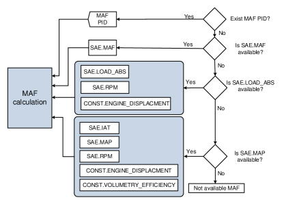
  Figure 4: Scheme of the different MAF calculation possibilities regarding fuel consumption calculation.

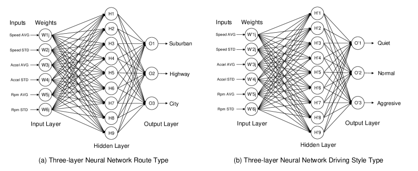
Figure 5: Schematic representation of the Three-layer Neural Networks used in the DrivingStyles Architecture.

4.2 Greenhouse gas emissions calculation

The most significant greenhouse gases are generated from direct combustion of carbon dioxide $CO_{2}$, Methane ($CH_{4}$), and Nitrous oxide ($N_{2}O$), among others. $CO_{2}$ is always generated when burning fuel that contains carbon. Since the carbon in the fuel is combined with the oxygen in the air: $C+O_{2}\rightarrow CO_{2}$, the amount of $CO_{2}$ can be calculated by the atomic masses of carbon and oxygen, and the carbon content of the fuel. The atomic mass of carbon is $12_{U}$ and oxygen is $16_{U}$, meaning that $CO_{2}=12_{U}+2\>\cdot\>16_{U}=44_{U}$. Burning 1kg of carbon produces $44/12\approx 3.67kg$ of $CO_{2}$ in complete combustion, and so the $CO_{2}$ emission of combustion is $3.67\>\cdot\>C_{c}\>\cdot\>m_{fuel}$ where $C_{c}=fuel\>carbon\>content\>(mass\>basis)$. Considering that the carbon content of diesel fuel is 85.7% the $CO_{2}$ emission when burning 1kg ($m_{fuel}=1kg$) of diesel fuel is:

$$m_{CO_{2}} = 3.67\>\cdot\>C_{c}\>\cdot\>m_{fuel}$$

$$m_{CO_{2}} = 3.67\>\cdot\>0.857\>\cdot\>1\left[kg\right]=3.15\>\left[kg/1kg\>fuel\right]$$

$$Density\>of\>diesel\>fuel\>is\>0.84\>\left[kg/l\right]$$

$$m_{CO_{2}} = 3.15\>\cdot{\left[kg\right]}\>\cdot\>0.84=2.64\>\left[kg/1l\>fuel\right]$$ (3)

Driving in a fuel-efficient manner can save fuel, money, and reduce greenhouse gas emissions. Among the factors that can affect fuel consumption, such as: vehicle age and condition, outside temperature, weather, and traffic conditions, we consider that driver behavior can be one of the most relevant parameter. Next, we provide detailed information about the neural network we proposed for characterizing driver styles.

5 Neural Networks-based data analysis

Neural networks [15] use artificial intelligence and automatic processing techniques to learn how to find patterns in data, thereby improving their success rate at making decisions of predictions. A learning algorithm is used to generate the neural network. For example, the driving style of each user and the type of route can be characterized from a well-defined set of rules and the ECU input variables.

There are many different learning algorithms such as backprop_momentum, Hebbian, or delta-rule, each one having its own advantages and disadvantages depending on the type of problems. In our project, we face a classification problem: starting from some input data, which in our case are the speed, acceleration, and revolutions per minute (rpm) of the engine, we intend to obtain as outputs the type of road and the driving style. The problem of classifying the driver behavior and the route type with a supervised learning is to find a function that best maps a set of inputs to its correct output. We tried several types of algorithms in this direction, including backpropagation, backprop-momentum, and batch backpropagation, and the results evidenced that backpropagation [13, 17] was the best algorithm for our study since it achieved the lowest sum of squared errors (SSE) in terms of prediction.

A data preprocessing stage is selected from all the possible input variables of the neural network. From all the possible data, we keep a subset of these variables. In practice, this subset is not the minimum; instead, it is a compromise between a manageable number (not too large) of variables and an acceptable network performance. In this work, after considering the many variables that can be obtained from the Electronic Control Unit (ECU), we have chosen to train the neural network using: the mean and standard deviation of speed, the vehicle acceleration, and the rpm value.

In all the vehicles used for testing, these variables are easily obtained. Other variables, such as the position of the throttle, which would provide important information for the neural network training, have to be rejected because not all manufacturers provide such information. The data input of each parameter is normalized between 0 and 1; this normalization should take into consideration the range of possible values. The schematic representation of our three-layer neural network can be seen in figures 5a, and 5b.

The application used for the creation and training of the neural networks required by this project is JavaNNS [16], a java version of the SNNS program from the University of T bingen.

First, an empty neural network was created, defining the number of entries mentioned previously, and the number of hidden nodes. A larger number of hidden nodes can improve the success rate, but has the negative effect of increasing the response time. On the contrary, with a large number of nodes, the network becomes a memory bank that can recall the training set to perfection, but does not perform well on samples that were not part of the training set. There are three output nodes for each neural network, one that characterizes the type of road (urban, suburban, or highway), and another one that characterizes the user’s driving style (quiet, normal, or aggressive), see figures 1a and 1b respectively.

Subsequently, we train the network with a total of 16038 samples, each representing a 3-second drive period (13.3 hours in total belonging to 7 drivers of different ages and sex). We initially adjust the learning rate to learning intervals of 0.2, and then modify this value to observe how the error affects the neural network (JavaNNS application [16] computes the mean square error in each learning iteration). The higher the learning rate, the greater the weight updating following each iteration; therefore, learning becomes faster, but it is prone to cause unwanted oscillations in the network. As the network training progresses, the number of learning cycles that take place in the tests is adjusted until the final trained network is obtained.

Once the neural network was successfully trained, the knowledge obtained was converted into C code, and this code was then integrated into our DrivingStyles platform. With the neural network already implemented, every time a route or route segment is selected, the system automatically returns the type of road, as well as the associated driving style. Figure 3 shows the results obtained by our neural network including the driving styles and route characterization of a particular route of one of our users.

Overall, with different traces analyzed, along with the drivers using our application, we have shown a correct classification of the different routes registered, both in terms of route types and driving styles, thus validating our proposed solution.

6 Experimental results and evaluation

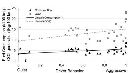
Figure 6: Chart of consumption and $CO_{2}$ in relation to the driving behavior.

In our project, we focus on characterizing the driving style of different drivers, and then measuring the associated fuel consumption variations. In order to achieve this objective, we rely on the collaboration of 534 drivers from around the world using our platform, including countries like India, Brazil, Central America, and Europe. In this particular study, we analyzed the behavior of 75 representative routes (each divided into 10 second periods) using the neural network described earlier. For each section, the neural network returns the corresponding driver behavior, and we combine this data with the fuel consumption data corresponding to that route.

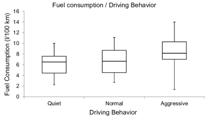
Figure 7: Box and whisker plot of Fuel Consumption/Driving Behavior.

We carried out several types of tests to validate our proposals. Figure 6 shows the fuel consumption and $CO_{2}$ emissions reported by different drivers classified according to their driving style. The results of this test show that a more aggressive driving behavior causes fuel consumption to increase significantly, while also increasing the generation of $CO_{2}$. To gain further insight into these correlations, Figure 7 displays the differences between quiet, normal, and aggressive driving behavior in terms of fuel consumption; aggressive drivers provoke fast starts and quick accelerations, driving at high engine revolutions, and causing sudden speed changes. Conversely, a quiet driving behavior would be smooth, without sudden speed changes or continuous gear shifts. It is clear that fuel consumption increases when the driver behavior becomes more aggressive, with average differences of up to 1.5 liters per 100km. In our experiments, an aggressive driver uses an average of 8 liters per 100km, and a quiet driver only 6.6 liters per 100km, meaning that the difference in terms of fuel consumption is not negligible, as the former may consume up to 20% more fuel depending on the driving style. Regarding $CO_{2}$ emissions, they may increase by 50%, going from 10 to 15Kg/100km, depending on whether drivers are quiet or aggressive.

7 Conclusions and future work

This paper presents our DrivingStyles platform, which integrates mobile devices with data obtained from the vehicle’s engine Electronic Control Unit (ECU) to characterize driver habits, as well as the associated fuel consumption and emissions. Our platform helps to promote a more ecological driving style by emphasizing on the relationship between driving style and fuel consumption, which has a clear and direct impact on the environment. It has been also demonstrated that the driving style is directly related to fuel consumption. Specifically, adopting an efficient driving style allows achieving fuel savings ranging from 15 to 20%. An aggressive driving style always results in a greater energy consumption and more $CO_{2}$ emissions, whereas smooth driving ends up providing a greater energy efficiency and reduced gas emissions. The application, which is available for free download in the DrivingStyle’s website and Google Play Store, achieved more than 5800 downloads from different countries in just a few months. This emphasizes the great interest about research on this topic. As future work, we intend to extend this platform by providing route recommendations based on real-time feedback about the congestion state of different alternative routes, as well as providing estimated greenhouse emissions for different routes.

jmeseguer.pdfJavier E. Meseguer(jmesegue@upv.es) is a researcher in the Institute for Molecular Imaging Instrumentation (I3M). He has been involved in Web, Cloud development and Grid Technologies in the past 12 years, participating in 14 National and European Research Projects. From 1999 to 2004 he worked as a consultant at PricewaterhouseCooper and IBM Global services in Madrid.

toh.pdfC. K. Toh received his Ph.D. degree in Computer Science from Cambridge University (1996) and earlier EE degrees from Manchester University (1991) and Singapore Polytechnic (1986). TRWTactical Systems Inc., USA. DARPA Deployable Ad Hoc Networks Program at Hughes Research Labs, USA. He is a Fellow of the British Computer Society (BCS), New Zealand Computer Society (NZCS), Hong Kong Institution of Engineers (HKIE), and Institution of Electrical Engineers (IEE). He is a recipient of the 2005 IEEE Institution Kiyo Tomiyasu Medal and the 2009.

CarlosCalafate.pdfCarlos T. Calafate (calafate@disca.upv.es) graduated with honors in Electrical and Computer Engineering at the University of Oporto (Portugal) in 2001. He received his Ph.D. degree in Computer Engineering from the Technical University of Valencia in 2006, where he has worked since 2005. He is currently an associate professor in the Department of Computer Engineering at the UPV, Spain. He is a member of the Computer Networks research group (GRC). His research interests include mobile and pervasive computing, security, and quality of service in wireless.

jucano.pdfJuan-Carlos Cano(jucano@disca.upv.es) received his M.Sc. and Ph.D. degrees in computer science from the Polytechnic University of Valencia (UPV) in 1994 and 2002, respectively. From 1995 to 1997 he worked as a programming analyst at IBM’s manufacturing division in Valencia. He is a full professor in the Department of Computer Engineering at UPV in Spain. His current research interests include power-aware routing protocols and quality of service for mobile ad hoc networks and pervasive computing.

pietro.pdfPietro Manzoni(pmanzoni@disca.upv.es) received his M.S. degree in computer science from the Universita degli Studi of Milan, Italy, in 1989 and the Ph.D. degree in computer science from the Polytechnic University of Milan, Italy, in 1995. He is a full professor in the Department of Computer Engineering at UPV in Spain. His research activity is related to wireless networks protocol design, modeling, and implementation.

References

- [1] International Organization for Standardization, Road vehicles, Diagnostic systems, Keyword Protocol 2000, 1999.
- [2] J.E. Meseguer, C.T. Calafate, J.C. Cano, and P. Manzoni “DrivingStyles: a smartphone application to assess driver behavior” 18th IEEE symposium on Computers and Communications (ISCC 2013).
- [3] J.E. Meseguer, C.T. Calafate, J.C. Cano, and P. Manzoni “Assessing the Impact of Driving Behavior on Instantaneous Fuel Consumption”. 2015 IEEE 12th Consumer Communications and Networking Conference (CCNC 2015)
- [4] A. Meintz, and M. Ferdowsi “Designing efficient hybrid electric vehicles”, IEEE Vehicular Technology Magazine, IEEE, Volume:4, Issue 2, June 2009.
- [5] U. Hernandez, A. Perallos, N. Sainz, and I. Angulo “Vehicle on board platform: Communications test and prototyping”, in Intelligent Vehicles Symposium (IV), 2010 IEEE, pp. 967-972, 2010.
- [6] E. Erikcsson “Independent driving pattern factors and their influence on fuel-use and exhaust emission factors” Transportation Research Part D: Transport, Elsevier, 325-345J, 2001.
- [7] H. Johansson, P. Gustafsson, M. Henke, and M. Rosengren “Impact of EcoDriving on emissions. International Scientific Symposium on Transport and Air Pollution”, Avignon France, 2003.
- [8] M. Kuhler, and D. Kartens “Improved driving cycle for testing automotive exhaust emissions”, SAE Technical Paper Series 780650. 1978.
- [9] M. Andr “Driving cycles development: Characterization of the methods”, SAE Technical Papers Series 961112, 1996 .
- [10] D.Y.C. Leung, D.J. Williams, “Modelling of Motor Vehicle Fuel Consumption and Emissions Using a Power-Based Model”, Environmental Monitoring and Assessment, 65:21–29, 2000.
- [11] COPERT III, “Computer programme to calculate emissions from road transport Methodology and emission factors” (Version 2.1), Technical report No 49.
- [12] S. Matsumoto, and H. Kawashima, “Fundamental study on effect of preceding vehicle information on fuel consumption reduction of a vehicle group”, Journal Communications Networks. 15, 173–178, 2013.
- [13] R. Hecht-Nielsen “Theory of the back propagation neural network - Neural Networks”. IJCNN, International Joint Conference, 1989.
- [14] “VR-Based Fuel Consumption Gauge”, Circuit Cellar magazine, Issue 183, pp. 59 - 67, October 2005.
- [15] S. Haykin “Neural Networks: A Comprehensive Foundation”, NY: Macmillan, p. 2, 1994.
- [16] Igor Fischer, Fabian Hennecke, Christian Bannes, and Andreas Zell “JavaNNS, Java Neural Network Simulator”, User Manual, Version 1.1.
- [17] Rangachari Anand, Kishan Mehrotra, Chilukuri K. Mohan, and Sanjay Ranka “Efficient Classification for Multiclass Problems Using Modular Neural Networks” IEEE