Fluctuations of Collective Coordinates and Convexity Theorems for Energy Surfaces

Abstract

Constrained energy minimizations of a many-body Hamiltonian return energy landscapes $e(b)$ where $b\equiv\langle B\rangle$ represents the average value(s) of one (or several) collective operator(s), $B$, in an “optimized” trial state $\Phi_{b}$, and $e\equiv\langle H\rangle$ is the average value of the Hamiltonian in this state $\Phi_{b}$. It is natural to consider the uncertainty, $\Delta e$, given that $\Phi_{b}$ usually belongs to a restricted set of trial states. However, we demonstrate that the uncertainty, $\Delta b$, must also be considered, acknowledging corrections to theoretical models. We also find a link between fluctuations of collective coordinates and convexity properties of energy surfaces.

1 Introduction

Collective coordinates [1] have been of central importance in descriptions of structure and reactions in atomic, molecular, and nuclear physics. They generate models with far less degrees of freedom than the true number of coordinates, $3A$, as needed for a microscopic description of a system of $A$ particles. Often, the system’s dynamics can be compressed into slow motions of a few collective degrees of freedom $B$, while the other, faster degrees can be averaged out. Also, for identical particles, such collective degrees can be one-body operators, $B=\sum_{i=1}^{A}\beta(\mathbf{r}_{i},\mathbf{p}_{i},\sigma_{i},\tau_{i}),$ where $\mathbf{r}_{i},\mathbf{p}_{i},\sigma_{i},\tau_{i}$ refer to the position, momentum, spin, and if necessary isospin, respectively, of particle $i$. The summation over $i$ provides for more inertia in $B$ than in the individual degrees $\beta_{i}$.

The concept of energy surfaces [2] has been as important. Given a “coordinate-like” collective operator $B$ and its expectation value $b\equiv\left\langle B\right\rangle$, most collective models use an energy function, $e(b)$, and also a $b$-dependent inertia parameter, that drive the collective dynamics. Keywords such as “saddles”, “barriers”, etc., flourish [2].

Simultaneously, it is often assumed that the function, $e(b),$ results from an energy minimization under constraint. Namely, while the system evolves through various values of $b$, it is believed to tune its energy to achieve a (local) minimum. This aspect of finding $e(b)$ is central to many fields of physics. To illustrate, consider a Hamiltonian, $H=\sum_{i}T_{i}+\sum_{i<j}V_{ij},$ where $T$ and $V$ denote the usual kinetic and interaction operators. Given a trial set of density operators, $\mathcal{D}$, in many-body space, normalized by $\text{Tr}\mathcal{D}=1$, the energy function $e(b)$ may be defined as,

$$e(b)=\inf_{\mathcal{D}\Rightarrow b}\text{Tr}\left\{H\mathcal{D}\right\},$$ (1)

where Tr is a trace in the many-body space for the $A$ particles. The constraint, $\mathcal{D}\Rightarrow b,$ enforces $\text{Tr}\left\{B\mathcal{D}\right\}=b.$

There are theories which do not use, a priori, an axiom of energy minimization for the “fast” degrees of freedom. Time-dependent Hartree-Fock (HF) [3] trajectories, generalizations with pairing, adiabatic versions [4], often show collective motions. Equations of motion [5] and/or a maximum decoupling [6] of “longitudinal” from “transverse” degrees, have also shown significant successes in the search for collective degrees, at the cost, however, of imposing a one-body nature of both collective coordinates and momenta and accepting state-dependence of these operators. Such approaches define an energy surface once trajectories of wave functions have been calculated. But they are not the subject of the present analysis. Herein, we focus on fixed operators constraining strict energy minimizations within a fixed basis for single-particle and many-body states. The questions arise: are those constraints themselves subject to fluctuations, and what would be the effect of those fluctuations on the energy minimization?

This is not a new question. The issue of constrained Hartree-Fock calculations was addressed in Ref. [7], which considered constrained Hartree-Fock calculations, and corrections to the energy surface. The issue has also been considered more recently in relation to high-energy $(e,e^{\prime}p)$ and $(p,2p)$ reactions [8], where fluctuations in the position vectors of the target nucleons involved in those processes were considered as going beyond the mean-field approximation assumed for the structure of the target nucleus.

Ideally, to define mathematically a function $e(b)$ of the collective coordinate, one should first diagonalize $B$ within the space provided by the many-body states available for calculations [9]. The resulting spectrum of $B$ should be continuous, or at least have a high density for that chosen trial space. Then, for each eigenvalue $b$, one should find the lowest eigenvalue, $e(b)$, of the projection of $H$ into that eigensubspace labeled by $b$.

In practice, however, one settles for a diagonalization of the constrained operator, $\mathcal{H}\equiv H-\lambda B$, where $\lambda$ is a Lagrange multiplier, or at least for a minimization of $\left\langle\mathcal{H}\right\rangle.$ Concomitantly, $B$ is assumed to have both upper and lower bounds, or that the constrained Hamiltonian, $\mathcal{H},$ always has a ground state. This returns the “free energy”, $\varepsilon(\lambda)\equiv\left\langle\mathcal{H}\right\rangle$. The label $b$ is no longer an eigenvalue but just an average value, $b=\left\langle B\right\rangle$. A standard Legendre transform of $\varepsilon(\lambda)$ then yields the “energy surface”, $e(b)$. This utilises the properties $d\varepsilon/d\lambda=-\text{Tr}\{B\mathcal{D}\}=-b$, and, $de/db=\lambda$. However we show in this work that constrained variation in a quantum system without additional precautions can raise at least two problems, namely: i) the parameter $b$ may no longer be considered as a well-defined coordinate for a collective model due to non-negligible fluctuations; we report cases where the uncertainties, $\Delta b$, can vitiate the meanings of both $b$ and $e(b)$; and ii) there is a link between strict minimization and the curvature properties of $e(b)$ when fluctuations are at work.

Our argument is based fundamentally on a few theorems, presented in Section II, but also illustrated using a few explicit models, which may be solved analytically or numerically. Such solutions for those simple models are presented in Section III. A discussion and conclusion make Section IV.

2 Theorems linking strict minimization and convexity

2.1 Preliminaries

Before proving such theorems, we must recall that, with Hartree-Fock (HF) and Hartree-Bogoliubov (HB) approximations, both convex and concave branches are obtained for $e(b)$ by the addition, in $\langle\mathcal{H}\rangle$ with the constraint term $-\lambda\left\langle B\right\rangle$, a square term, $\frac{1}{2}\mu\left\langle B\right\rangle^{2}$, $\mu>0$ [7, 10, 11, 12], allowing for adjustable values of $\lambda$ and sometimes $\mu$. It must be stressed that $\langle B\rangle^{2}$ differs from $\langle B^{2}\rangle.$ It must also be stressed that such mean-field results are approximations, and that all such methods using a quadratic term in the original function, while stabilizing the numerical procedure, amount to using an effective Lagrange multiplier. Typically, when the “completed” functional, $\langle H\rangle+\frac{1}{2}\mu\langle B\rangle^{2}-\lambda\langle B\rangle$, is minimized by a trial function $\phi$ in a mean-field approximation, any bra variation, $\langle\delta\phi|$, induces the condition,

$$\left\langle\delta\phi\left|H\right|\phi\right\rangle+\left(\mu\left\langle B\right\rangle-\lambda\right)\left\langle\delta\phi\left|B\right|\phi\right\rangle=0,$$ (2)

and a similar result holds for any ket variation. Clearly, this means that the combination, $\langle H\rangle-\Lambda\,\langle B\rangle$, with the effective Lagrange multiplier, $\Lambda=\lambda-\mu\,\langle B\rangle$, has been made stationary (but not necessarily minimal). We, therefore, consider the generic form, $\mathcal{H}=H-\lambda B$, in the following discussions.

As far as we are aware, none of the literature on energy surfaces obtained with such quadratic cost functions is concerned with uncertainties in the collective labels. However, any $e(b)$ may find an increase in its uncertainty if $b$ itself, the expectation value of a quantum operator, is subject to large fluctuations. A surprising observation of the present work is that the convexity properties of energy surfaces and uncertainties in the collective coordinates are related. This work clarifies the situation.

2.2 Convexity from a convex domain of trial states

Assume that minimization under constraint is performed in a convex domain of many-body density matrices $\mathcal{D}$. Namely, if $\mathcal{D}_{1}$ and $\mathcal{D}_{2}$ are trial states, any combination, $\mathcal{D}_{m}=\nu\mathcal{D}_{1}+(1-\nu)\mathcal{D}_{2}$, with $0<\nu<1$, is also a trial state. The constraint operator can be one bounded operator $B$, or several such operators, $B_{1},\dots,B_{N}$, or an infinite number of them, such as, for density functionals, local field operators, $\psi_{r}^{\dagger}\psi_{r}$, labeled by a continuous position $r$. For notational simplicity, we denote the set of constraint operators by one symbol only, $B$, and the corresponding expectation values as $b\equiv{\rm Tr}(B\mathcal{D})$. We call “slice $b$” the set of all those $\mathcal{D}$ returning a given $b$. We also assume, for simplicity, that, inside “slice $b$”, the minimum $e(b)$ of $\mathrm{Tr}(H\mathcal{D})$ is reached for a state $\mathcal{D}_{mb}$, which is non-degenerate.

Then, given two constraint values $b_{1}$ and $b_{2}$, with the associated minimalizing states $\mathcal{D}_{m1}$ and $\mathcal{D}_{m2}$, it is clear that the interpolating state, $\mathcal{D}_{mix}=\nu\mathcal{D}_{m1}+(1-\nu)\mathcal{D}_{m2}$, returns both constraint and energy values, $b_{mix}=\nu b_{1}+(1-\nu)b_{2}$ and $e_{mix}=\nu e(b_{1})+(1-\nu)e(b_{2})$. However, there is no reason why $\mathcal{D}_{mix}$ should be the energy minimizing state inside that slice labeled by $b_{mix}$. Hence, by necessity, the energy minimum inside the slice obeys the inequality, $e(b_{mix})\leq e_{mix}$. In short, $e$ is necessarily a convex function (or functional).

Experimental tables of ground state energies $E_{A}$ are incompatible (see Ref. [13]) with such a convexity if a density functional is requested to be universal in terms of a particle number $A$. Indeed, there are many cases where $E_{A}\geq(E_{A-1}+E_{A+1})/2$. In such a situation, a convex functional, with a mixed density, $(\rho_{A-1}+\rho_{A+1})/2$, hence a fluctuation $\Delta A=1$, will return a lower energy than $E_{A}$. See Ref. [13] for ways to “make Nature convex”.

Many practical calculations of spectra or energy surfaces use at first mean field methods, where trial states do not belong to a convex domain. For instance, a weighted sum of two Slater determinants usually does not make a Slater determinant. A similar statement holds for HB states. The question of convexity [14], however, and its relation to fluctuations, often remains.

2.3 A general theorem

Given a constrained Hamiltonian, $H-\lambda B$, consider a solution branch $\mathcal{D}(\lambda)$, expanding up to second order, assuming that the manifold of solutions is suitably analytic,

$$\mathcal{D}(\lambda+d\lambda)=\mathcal{D}(\lambda)+d\lambda(d\mathcal{D}/d\lambda)+(d\lambda^{2}/2)(d^{2}\mathcal{D}/d\lambda^{2}).$$ (3)

In those cases where pure states, ${\cal D}=|\phi\rangle\langle\phi|$, are used, the wave function of interest is assumed to be analytical, and, clearly, $d{\cal D}/d\lambda=|\phi\rangle\langle d\phi/d\lambda|+|d\phi/d\lambda\rangle\langle\phi|$, and also, $d^{2}{\cal D}/d\lambda^{2}=|\phi\rangle\langle d^{2}\phi/d\lambda^{2}|+2\,|d\phi/d\lambda\rangle\langle d\phi/d\lambda|+|d^{2}\phi/d\lambda^{2}\rangle\langle\phi|$.

The stationarity and minimality of $\text{Tr}\left\{\mathcal{H}\mathcal{D}\right\}$ with respect to any variation of $\mathcal{D},$ and in particular with respect to that variation, $\mathcal{D}(\lambda+d\lambda)-\mathcal{D}(\lambda),$ induce,

$$\text{Tr}\left\{\mathcal{H}d\mathcal{D}/d\lambda\right\} =0,$$

$$\text{Tr}\left\{\mathcal{H}d^{2}\mathcal{D}/d\lambda^{2}\right\} \geq 0.$$ (4)

The free energy $\varepsilon$ is also stationary for $\mathcal{D}(\lambda+d\lambda)$, but the Hamiltonian is now, $\mathcal{H}(\lambda)-B\,d\lambda$, and the derivative of the state is, $d\mathcal{D}/d\lambda+d\lambda(d^{2}\mathcal{D}/d\lambda^{2})+\mathcal{O}(d\lambda^{2})$, hence,

$$\text{Tr}\left\{\left(\mathcal{H}-Bd\lambda\right)\left[d\mathcal{D}/d\lambda+d\lambda(d^{2}\mathcal{D}/d\lambda^{2})+\mathcal{O}(d\lambda^{2})\right]\right\}=0.$$ (5)

The zeroth order of this, Eq. (5), is, $\text{Tr}\left\{\mathcal{H}d\mathcal{D}/d\lambda\right\}$. It vanishes, because of the first of Eqs. (4). The first order, once divided by $d\lambda$, gives,

$$-\text{Tr}\left\{Bd\mathcal{D}/d\lambda\right\}=-\text{Tr}\left\{\mathcal{H}d^{2}\mathcal{D}/d\lambda^{2}\right\}.$$ (6)

The left-hand side of Eq. (6) is nothing but the second derivative, $d^{2}\varepsilon/d\lambda^{2}$. The right-hand side is semi-negative-definite, because of the second of Eqs. (4). Hence, the plot of $\varepsilon(\lambda)$ is a concave curve and the plot of its Legendre transform, $e(b)$, is convex. (Other papers [13] have the opposite sign convention of the second derivative to define convexity.) With the present sign convention, strict minimization of $\langle{\cal H}\rangle$ necessarily induces convexity of $e(b)$. Any concave branch for $e(b)$ demands an explanation.

Note that this proof does not assume any specification of $\mathcal{D}(\lambda)$, whether it is constructed either from exact or approximate eigenstates of $\mathcal{H}$. Therefore strict minimization of $\langle(H-\lambda B)\rangle$ can only return convex functions $e(b)$. Maxima are impossible. In the generalization where several collective operators $B_{1},\dots,B_{N}$, are involved, convexity still holds, so saddles are also excluded. Hence, only an absolute minimum is possible. (However, we shall recall below how to overcome the paradox: by keeping small enough [15] the fluctuations of the collective coordinate(s), one can deviate from convexity, and more important, validate the quality of the representation provided by branches $\mathcal{D}(\lambda)$.)

2.4 Same theorem, for exact solutions

Let $\psi(\lambda)$ be the ground state of $\mathcal{H}$. (For the sake of simplicity, we assume that there is no degeneracy.) The corresponding eigenvalue, $\varepsilon(\lambda)$, is stationary with respect to variations of $\psi$, among which is the “on line” variation, $d\lambda\,(d\psi/d\lambda)$, leading to the well-known first derivative, $d\varepsilon/d\lambda=-b\equiv-\left\langle\psi\left|B\right|\psi\right\rangle$. Consider the projector, $Q=1-\left|\psi\right\rangle\left\langle\psi\right|.$ Brillouin-Wigner theory yields the first derivative of $\psi$, viz.

$$\frac{d\left|\psi\right\rangle}{d\lambda}=-\frac{Q}{\varepsilon-Q\mathcal{H}Q}B\left|\psi\right\rangle.$$ (7)

This provides the second derivative of $\varepsilon,$

$$-\frac{db}{d\lambda}\equiv-\frac{d}{d\lambda}\left\langle\psi\left|B\right|\psi\right\rangle=2\left\langle\psi\left|B\frac{Q}{\varepsilon-Q\mathcal{H}Q}B\right|\psi\right\rangle.$$ (8)

Since the operator $(\varepsilon-Q\mathcal{H}Q)$ is clearly negative-definite, the eigenvalue, $\varepsilon$, is a concave function of $\lambda$. It is trivial to prove that the same concavity holds for the ground state eigenvalue $\varepsilon(\lambda_{1},\dots,\lambda_{N})$ if several constraints, $B_{1},\dots,B_{N}$, are used. If, moreover, a temperature $T$ is introduced, the thermal state, $\mathcal{D}=\exp\left[-\mathcal{H}/T\right]/\text{Tr}\exp\left[-\mathcal{H}/T\right],$ replaces the ground state projector and the free energy also contains the entropy contribution, $-TS,$ where $S=-\text{Tr}\left\{\mathcal{D}\ln\mathcal{D}\right\}$. A proof of the concavity of the exact $\varepsilon(\lambda_{1},\dots,\lambda_{N};T)$ is also easy [16].

At $T=0,$ the usual Legendre transform expresses the energy, $e\equiv\left\langle\psi\left|H\right|\psi\right\rangle$, in terms of the constraint values, $b_{1},\dots,b_{N}$, rather than the Lagrange multipliers. For simplicity, consider one constraint only; the generalization to $N>1$ is easy. Since $e\equiv\varepsilon+\lambda b$, then $de/db=\lambda$, a familiar result for conjugate variables. Furthermore, the second derivative, $d^{2}e/db^{2},$ reads, $d\lambda/db=1/(db/d\lambda)$. From Eq. (8), the derivative, $db/d\lambda$, is positive-definite. Accordingly, $e$ is a convex function of $b$. Now, if $T>0$, the Legendre transform instead generates a reduced free energy, $\eta\equiv(e-TS)$, a convex function of the constraint value(s). An additional Legendre transform returns $e$ alone, as a convex function of the constraint(s) and $S$.

Let $b_{-}$ and $b_{+}$ be the lowest and highest eigenvalues of $B.$ When $\lambda$ runs from $-\infty$ to $+\infty,$ then $b$ spans the interval, $[b_{-},b_{+}]$. There is no room for junctions of convex and concave branches under technical modifications as used by Refs. [7, 10, 11, 12]. For every exact diagonalization of $\mathcal{H}$, or exact partition function, convexity sets a one-to-one mapping between $b$ in this interval and $\lambda$. More generally, with exact calculations, there is a one-to-one mapping between the set of Lagrange multipliers, $\left\{\lambda_{1},\dots,\lambda_{N}\right\},$ and that of obtained values, $\left\{b_{1},\dots,b_{N}\right\}$, of the constraints. Convexity, in the whole obtained domain of constraint values, imposes a poor landscape: there is one valley only.

We tested this surprising result with several dozens of numerical cases, where we used random matrices for $H$ and $B,$ with various dimensions. As an obvious precaution, we eliminated those very rare cases where both $H$ and $B$ turned out, by chance, to be block matrices with the same block structure; such cases give rise to level crossings and degeneracies. Then every remaining situation, without exception, confirmed the convexity of $e$. Figure 1 shows all branches of $e(b)$ for $H=\left[\begin{smallmatrix}-3&0&3&2\\ 0&5&-4&4\\ 3&-4&-4&5\\ 2&4&-5&-1\end{smallmatrix}\right]$ and $B=\left[\begin{smallmatrix}0&-2&0&3\\ -2&2&-2&-2\\ 0&-2&-4&-1\\ 3&-2&-1&7\end{smallmatrix}\right]$ for instance. Such branches are easily derived algebraically [17] from the polynomial, $P\equiv\det(H-\lambda B-\varepsilon)$. The convexity of the ground state branch is transparent. Clear also are its infinite derivatives when $b$ reaches $b_{-}=-4.83$ and $b_{+}=9.60$, and the vanishing derivative at the point corresponding to the unconstrained ground state, where $b=-2.69$ and $e=e_{-}=-9.71$.

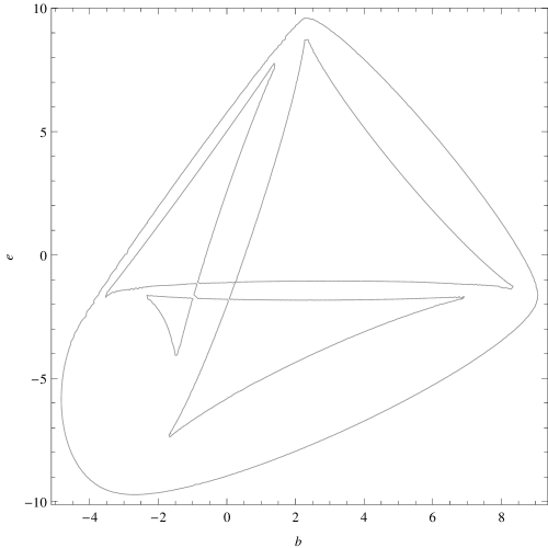
Figure 1: Branches obtained for $e(b)$ by algebraic elimination of the Lagrange multiplier $\lambda$ between $b(\lambda)$ and $e(\lambda)$ in a toy case with $4\times 4$ matrices. Convexity of the ground state branch.

2.5 Same theorem, for approximations via constrained HF calculations

Consider now energy surfaces obtained from approximations. Typically, one uses a HF or HB calculation, at zero or finite $T$. Trial states in such methods span a nonlinear manifold; indeed, a sum of two determinants is usually not a determinant. Let $\mathcal{D}(\lambda)$ denote one $A$-body density operator where, within such nonlinear approximations, a minimum, $\varepsilon(\lambda)$, of $\text{Tr}\left\{\mathcal{H}\mathcal{D}\right\}$ or of $\left(\text{Tr}\left\{\mathcal{H}\mathcal{D}\right\}-TS\right)$, is reached. It may be degenerate, but, in any case, it is stationary for arbitrary variations $\delta\mathcal{D}$ within the set of trial states. Accordingly, the first derivative again reads, $d\varepsilon/d\lambda=-b\equiv-\text{Tr}\left\{B\mathcal{D}\right\}$. Then, if a Legendre transform holds, defining $\eta\equiv\varepsilon+\lambda b$ in terms of $b$, the same argument that was used for the exact case again yields, $d\eta/db=\lambda$. With $N$ constraints, the gradient of $\eta$ in the domain spanned by $\left\{b_{1},\dots,b_{N}\right\}$ is the vector $\left\{\lambda_{1},\dots,\lambda_{N}\right\}$.

To discuss second derivatives, consider, for instance, HF calculations, where $A$-body density operators are dyadics of determinants, $\mathcal{D}=\left|\phi\right\rangle\left\langle\phi\right|$. Norm-conserving variations of an HF solution, $\phi$, can be parametrized as, $\left|\delta\phi\right\rangle=\exp(iX\delta\alpha)\left|\phi\right\rangle,$ with $X$ an arbitrary particle-hole Hermitian operator, and $\delta\alpha$ an infinitesimal coefficient. Under such a variation in the neighborhood of a HF solution, the first and second order variations of the free energy, $\varepsilon\equiv\text{Tr}\left\{\mathcal{H}\exp(iX\delta\alpha)\mathcal{D}\exp(-iX\delta\alpha)\right\}$, read,

$$\delta\varepsilon=i\delta\alpha\text{Tr}\left\{\left[\mathcal{H},X\right]\mathcal{D}\right\}=0,$$ (9)

and

$$\delta^{2}\varepsilon=-\left(\delta\alpha^{2}/2\right)\text{Tr}\left\{\left[\left[\mathcal{H},X\right],X\right]\mathcal{D}\right\}\geq 0,$$ (10)

respectively. If $\mathcal{D}$ is a HF solution, the first order vanishes $\forall X.$ Since only those solutions that give minima are retained, the second order variation of $\varepsilon$ is semi-positive-definite, $\forall X$ again. Now, when $\mathcal{H}$ receives the variation, $-Bd\lambda$, there exists a particle-hole operator, $Y$, a special value of $X$, that, with a coefficient $d\lambda$, modifies the solution. This reads $\left|\Phi\right\rangle=\exp(iYd\lambda)\left|\phi\right\rangle.$ Simultaneously, those particle-hole operators that refer to this new Slater determinant $\Phi$ become $\mathcal{X}=\exp(iYd\lambda)X\exp(-iYd\lambda)$. The new energy is,

$$\varepsilon_{Y}=\text{Tr}\left\{\exp(-iYd\lambda)(\mathcal{H}-Bd\lambda)\exp(iYd\lambda)\mathcal{D}\right\}.$$ (11)

The stationarity condition, Eq. (9), becomes,

$$0 =\text{Tr}\left\{\exp(-iYd\lambda)\left[(\mathcal{H}-Bd\lambda),\mathcal{X}\right]\exp(iYd\lambda)\mathcal{D}\right\}$$

$$=\text{Tr}\left\{\left[\exp(-iYd\lambda)(\mathcal{H}-Bd\lambda)\exp(iYd\lambda),X\right]\mathcal{D}\right\}.$$ (12)

The zeroth order in $d\lambda$ of this, Eq. (12), reads, $\text{Tr}\left\{\left[\mathcal{H},X\right]\mathcal{D}\right\}$, and vanishes $\forall X$, because of Eq. (9). Then the first order in $d\lambda$ gives, again $\forall X$,

$$\text{Tr}\left\{\left[B,X\right]\mathcal{D}\right\}=i\text{Tr}\left\{\left[\left[\mathcal{H},Y\right],X\right]\mathcal{D}\right\}.$$ (13)

The second derivative is,

$$d^{2}\varepsilon/d\lambda^{2} =-(d/d\lambda)\text{Tr}\left\{\exp(-iYd\lambda)B\exp(iYd\lambda)\mathcal{D}\right\}$$

$$=-i\text{Tr}\left\{\left[B,Y\right]\mathcal{D}\right\}.$$ (14)

Upon taking advantage of Eq. (13), for $Y$ as a special case of $X,$ this becomes,

$$d^{2}\varepsilon/d\lambda^{2}=\text{Tr}\left\{\left[\left[\mathcal{H},Y\right],Y\right]\mathcal{D}\right\},$$ (15)

the right-hand side of which is semi-negative-definite, see Eq. (10). The solution branch obtained when $\lambda$ runs is, therefore, concave. Its Legendre transform is convex.

2.6 About concave branches

Let us return to the “quadratic cost” function, that redefines the “free energy” to be minimized, $\mathcal{E}$, as, $\mathcal{E}=\langle H\rangle+\frac{1}{2}\mu\langle B\rangle^{2}-\lambda\langle B\rangle$, or, in a shorter notation, $\mathcal{E}=e+\frac{1}{2}\mu b^{2}-\lambda b$. Let the positive number $\mu$ be kept constant, allowing $\lambda$ to vary. It is easy to show again that $d\mathcal{E}/d\lambda=-b$. But now one finds that, $de/db=\Lambda\equiv\lambda-\mu b$, where the effective Lagrange multiplier $\Lambda$ is that noticed at the stage of Eq. (2). Assume again that variational solutions are analytic with respect to $\lambda$. For the sake of simplicity, use wave functions $\phi$ rather than density operators, hence $\mathcal{D}=|\phi\rangle\langle\phi|$. The analog of Eq. (3) reads, $\phi(\lambda+d\lambda)=\phi+d\lambda\,\phi^{\prime}+\frac{1}{2}(d\lambda)^{2}\,\phi^{\prime\prime}$, with short notations for derivatives of $\phi$. The stationarity of $\mathcal{E}$ then reads,

$$0=\mathcal{E}^{\prime}\equiv\langle\phi^{\prime}|(H-\Lambda B)|\phi\rangle+\langle\phi|(H-\Lambda B)|\phi^{\prime}\rangle\,.$$ (16)

If this “quadratic cost” $\mathcal{E}$ is a strict minimum with respect to variations of $\phi$, one finds,

$$0<\mathcal{E}^{\prime\prime}\equiv\langle\phi^{\prime\prime}|\,(H-\Lambda B)\,|\phi\rangle+2\langle\phi^{\prime}|\,(H-\Lambda B)\,|\phi^{\prime}\rangle$$

$$+\,\langle\phi|\,(H-\Lambda B)\,|\phi^{\prime\prime}\rangle+\mu\,(\,\langle\phi^{\prime}|B|\phi\rangle+\langle\phi|B|\phi^{\prime}\rangle\,)^{2}\,.$$ (17)

When $\lambda$ becomes $\lambda+d\lambda$, the derivative of the wave function becomes $(\phi^{\prime}+d\lambda\,\phi^{\prime\prime})$ and the functional to be minimized receives an additional contribution, $-d\lambda\,\langle B\rangle$. Then the stationarity condition at $\phi(\lambda+d\lambda)$ becomes,

$$0=(\mathcal{E}^{\prime}+d\lambda\,\mathcal{E}^{\prime\prime})-d\lambda\,(\,\langle\phi^{\prime}|B|\phi\rangle+\langle\phi|B|\phi^{\prime}\rangle\,)\,.$$ (18)

This simplifies into, $\mathcal{E}^{\prime\prime}=db/d\lambda$, since $\mathcal{E}^{\prime}=0$, see Eq. (16), and since, simultaneously, $db/d\lambda=\langle\phi^{\prime}|B|\phi\rangle+\langle\phi|B|\phi^{\prime}\rangle$. Furthermore, since $\mathcal{E}^{\prime\prime}>0$, see Eq. (17), and since we know that $d\mathcal{E}/d\lambda=-b$, we find that $d^{2}\mathcal{E}/d\lambda^{2}=-\mathcal{E}^{\prime\prime}$, a negative quantity. The function, $\mathcal{E}(\lambda)$, is, therefore, necessarily concave if a strict minimization of $\mathcal{E}$ has been performed in the domain of trial states.

As stated at the beginning of this Subsection, the “energy surface” function, $e(b)$, now obeys the condition, $de/db=\lambda-\mu\,b$, hence $d^{2}e/db^{2}=d\lambda/db-\mu$. While we found that $d\lambda/db=1/(db/d\lambda)=1/\mathcal{E}^{\prime\prime}$ is a positive quantity, the term, $-\mu$, competes with $d\lambda/db$ and may induce negative values of $d^{2}e/db^{2}$, hence concave regions in the plot of $e(b)$, where, incidentally, the second derivative, $d^{2}e/db^{2}$, cannot be more negative than $-\mu$.

Consider two solutions, $\phi_{1}$, $\phi_{2}$, generating two points, $(b_{1},e_{1})$, $(b_{2},e_{2})$, that are separated by an inflection point of $e(b)$ and that show the same derivative, $\Lambda=(de/db)_{1}=(de/db)_{2}$, in other words, $\lambda_{1}-\mu b_{1}=\lambda_{2}-\mu b_{2}.$ Denote $\phi_{1}$ the lower energy solution, hence $e_{1}<e_{2}$. Then $\phi_{2}$, compared with $\phi_{1}$, is an excited solution of the variational stationarity problem for the same constrained Hamiltonian, $H-\Lambda B$, that drives $\phi_{1}$. For the sake of the argument, assume that $b_{1}<b_{2}$. Then along the convex branch of $e(b)$, the value of $\Lambda$ increases when $b$ increases, and, when $b$ decreases along the concave branch, the value of $\Lambda$ also increases. When one reaches the inflection point, $(b_{i},e_{i})$, a maximum value, $\Lambda_{i}$, is reached. One must conclude that the two, formerly distinct solutions, $\phi_{1}(\Lambda)$ and $\phi_{2}(\Lambda)$, do not cross and, rather, smoothly fuse into a unique solution $\phi(\Lambda_{i})$. This is a very unlikely situation for exact solutions, namely eigenstates, as is well known. Only approximations can afford such an anomaly. (Notice also that, because $H-\Lambda B$ is assumed bounded from below, $\forall\Lambda$, there will exist a stationary solution $\phi_{+}$ for any multiplier $\Lambda_{+}>\Lambda_{i}$, even infinitesimally close to $\Lambda_{i}$. Then one must accept that $\Phi_{+}$ and $\Phi_{i}$ strongly differ from each other.)

The zoo of stationary solutions of approximate methods such as mean field methods (non linear!) can be rich enough to accommodate such singularities. This makes a paradox: would non-linear approximations generate a more flexible, physical tool than exact solutions? “Phase transitions”, a somewhat incorrect wording for a finite system, are sometimes advocated to accept continuing branches of energy minima into metastable branches. But this definitely claims some caution with the axiom of strict energy minimization to freeze fast degrees. This need for excited solutions in constrained mean field calculations, namely two solutions for the same value of a Lagrange multiplier to describe both sides of an inflection point of the barrier, is well known and used. See in particular [10, 11], where a tangent parabola rather than a tangent straight line is used to explore an energy surface by mean field methods.

2.7 Bimodal solutions in mean field approximations

Besides the caution about the “fast degree minimization hypothesis” one should consider whether such mean field solutions, in convex or concave branches, might be vitiated by large uncertainties for $b$. The following solvable models give a preliminary answer.

Consider $N$ identical, 1-D fermions with Hamiltonian,

$$H=\sum_{i=1}^{N}p_{i}^{2}/(2m)+M\omega^{2}R^{2}/2+\sum_{i>j=1}^{N}v_{ij},$$ (19)

where $R=\sum_{i}r_{i}/N$ is the center-of-mass (c.m.) position, $p_{i},r_{i},m$ denote the single particle momentum, position and mass, respectively, of each fermion, and $M=Nm$ is the total mass. The c.m. momentum is, $P=\sum_{i}p_{i}.$ We use a system of units such that $\hbar=m=\omega=1,$ where $\omega$ denotes the frequency of the c.m. harmonic trap. The interaction, $v,$ is set as Galilean invariant and so is the sum, $V=\sum_{i>j}v_{ij}.$ In the following, $v$ is taken as a spin and isospin independent and local force, $v_{ij}=v(|r_{i}-r_{j}|).$

The collective operator we choose to constrain $H$ is a half sum of “inertia” (mass weighted square radii), $B=\sum_{i=1}^{N}mr_{i}^{2}/2$. The constrained Hamiltonian then reads,

$${\cal H}=\sum_{i}p_{i}^{2}/(2m)+M\omega^{2}R^{2}/2+\sum_{i>j}v_{ij}-\lambda\sum_{i}mr_{i}^{2}/2.$$ (20)

Let $\xi_{1}=r_{2}-r_{1},$ $\xi_{2}=r_{3}-(r_{1}+r_{2})/2,$ …, $\xi_{N-1}=r_{N}-(r_{1}+r_{2}+\dots+r_{N-1})/(N-1)$ denote the usual Jacobi coordinates with $\Pi_{\alpha}$ and $\mu_{\alpha}$, $\alpha=1,\dots,(N-1)$, the corresponding momenta and reduced masses. In this Jacobi representation the constraint becomes, $B=MR^{2}/2+\sum_{\alpha}\mu_{\alpha}\xi_{\alpha}^{2}/2.$ Accordingly, the constrained Hamiltonian decouples as a sum of a c.m. harmonic oscillator,

$$\mathcal{H}_{\text{c.m.}}=\frac{P^{2}}{(2M)}+\frac{1}{2}M\Omega^{2}R^{2},\;\;\;\Omega^{2}=\omega^{2}-\lambda,$$ (21)

provided $\lambda<\omega^{2}$, and an internal operator,

$$\mathcal{H}_{\text{int}}=\sum_{\alpha}\left[\Pi_{\alpha}^{2}/(2\mu_{\alpha})-\lambda\mu_{\alpha}\xi_{\alpha}^{2}/2\right]+V.$$ (22)

With the present power of computers and present experience with Faddeev(-Yakubovsky) equations, this choice of $\mathcal{H}$ and $B$, with its ability to decouple, provides soluble models with, typically, $N=2,3,4$. (Decoupling also occurs if $B$ is a quadrupole operator.) Exact solutions can thus be compared with mean field approximations and validate, or invalidate, the latter. Here, however, we are not interested in the comparison, but just in properties of the mean field solutions as regards $B$.

For this, as long as $N$ does not exceed $4$, we assume that the Pauli principle is taken care of by spins and isospins, understood in the following, and that the space part of the mean field approximation is a product, $\phi=\prod_{i}\varphi(r_{i}),$ of identical, real and positive parity orbitals. The corresponding Hartree equation reads,

$$\left[\frac{p^{2}}{2m}+\Lambda r^{2}+u(r)\right]\varphi(r)=\varepsilon_{sp}\varphi(r),$$ (23)

with $u(r)=(N-1)\int_{-\infty}^{\infty}v(r-s)[\varphi(s)]^{2}$ and $\Lambda=M\omega^{2}/(2N^{2})-\lambda m/2.$ The term, $M\omega^{2}/(2N^{2}),$ clearly comes from the c.m. trap. The same trap induces a two-body operator, $M\omega^{2}\sum_{i\neq j}r_{i}r_{j}/(2N^{2}),$ which cannot contribute to the Hartree potential, $u,$ since every dipole moment, $\left\langle r_{j}\right\rangle$, identically vanishes here.

Once $\varphi$ and $\varepsilon_{sp}$ are found, one obtains the free energy, $\varepsilon_{\text{Hart}}=\langle\mathcal{H}\rangle=N\varepsilon_{sp}-N\left\langle\varphi\left|u\right|\varphi\right\rangle/2$, then the value of the constraint, $\left\langle B\right\rangle_{\text{Hart}}=Nm\left\langle\varphi\left|r^{2}\right|\varphi\right\rangle/2,$ and the square fluctuation, $(\Delta b)^{2}_{\text{Hart}}=Nm^{2}\left(\left\langle\varphi\left|r^{4}\right|\varphi\right\rangle-\left\langle\varphi\left|r^{2}\right|\varphi\right\rangle^{2}\right)/4.$ The physical energy, $e_{\text{Hart}}(b),$ in this Hartree approximation, clearly obtains by adding $\lambda\langle B\rangle_{\text{Hart}}$ to $\varepsilon_{\text{Hart}}.$

We show now, among many cases we studied, Hartree results when $v_{ij}=-2[\exp(-2(r_{i}-r_{j}+8)^{2})+\exp(-2(r_{i}-r_{j}-8)^{2})+2\exp(-2(r_{i}-r_{j}+4)^{2})+2\exp(-2(r_{i}-r_{j}-4)^{2})+\exp(-2(r_{i}-r_{j})^{2})],$ see Fig. 2.

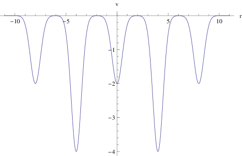
Figure 2: An interaction giving multimodal Hartree solutions.

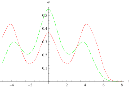
Figure 3: Dashes, Hartree orbital $\varphi(r)$ if $N=2,$ $\lambda=.47$ for the interaction shown in Fig. 2. Dots, the same for $\lambda=.55.$

Figure 4: Same Hartree model. $\Delta b$ as a function of $\langle B\rangle.$

The results shown in Figs. 2-4 correspond to $N=2$. Similar results hold with $N=3,4$. Orbitals $\varphi$ are expanded in the first 11 even states of the standard harmonic oscillator. The only difference between the two orbitals shown in Fig. 3 is the value of $\lambda$. Both orbitals, and many other ones, when $\lambda$ runs, show a bimodal structure, their left-hand-side and right-hand-side bumps being equivalent with respect to the even observable, $B\propto r^{2}$. Whether $N=2$, $3$, or $4$, we found many cases where the value of $\langle B\rangle$ has nothing to do with the positions of the peaks of $\varphi$. The bad quality induced by the corresponding uncertainties is illustrated by Fig. 4. Therefore, little trust is available for the energy curve, $e_{Hart}(b)$, that results from this model.

3 Models showing the existence and extent of quantum fluctuations of collective coordinates

We now turn our attention to illustrating the effects of fluctuations of collective coordinates, as discussed above, with various examples.

3.1 Fluctuation of the mean square radius in a harmonic oscillator shell model

Consider $A$ fermions with Hamiltonian, $H=\frac{1}{2}\sum_{i=1}^{A}(p_{xi}^{2}+p_{yi}^{2}+p_{zi}^{2}+x_{i}^{2}+y_{i}^{2}+z_{i}^{2})$, or, in a shorter notation, $H=\sum_{i}(p_{i}^{2}+r_{i}^{2})/2$. Ignore spin (and isospin) and fill completely each shell up to that one with energy $n+\frac{3}{2}$. It is trivial that the sequence of individual shell populations reads, $1,3,6,\dots,(n+1)(n+2)/2$, and that, when all shells up to and including “shell $n$” are filled, the particle number reads, $A=(n+1)(n+2)(n+3)/6$. Denote $\phi$ that Slater determinant made of such $(n+1)$ filled shells and choose now the collective operator, $B=A^{-1}\sum_{i=1}^{A}r_{i}^{2}$. By definition, $b\equiv\langle B\rangle$ represents the square of an average radius, $\bar{r}=\sqrt{b}$.

For the sake of mathematical rigour, it might be necessary to redefine $B$ with a cut-off, such as, $B_{c}=\sum r_{i}^{2}\exp(-r_{i}^{2}/R_{c}^{2})$, with $R_{c}$ significantly larger than atomic, molecular or nuclear radii, to ensure that constrained Hamiltonians, $H-\lambda B_{c}$, do have a ground state if $\lambda>0$. But this technicality can be neglected in practice, with calculations using a large but finite basis of finite range variational states.

Each shell with index $m,\ m=0,\dots,n$, contributes $A^{-1}(m+3/2)(m+1)(m+2)/2$ to $\langle\phi|B|\phi\rangle$, hence a total $\langle B\rangle=A^{-1}(n+1)(n+2)^{2}(n+3)/8$. Consider now $\langle B^{2}\rangle$, to calculate the fluctuation. Let $h$ be those states filled in $\phi$ and $P$ the other eigenstates of $H$. The one-body operator $B$ can excite at most one-particle-one-hole states when acting upon $\phi$, hence,

$$\langle B^{2}\rangle=\langle\phi|B|\phi\rangle\langle\phi|B|\phi\rangle+\sum_{Ph}\langle\phi|B|\phi_{Ph}\rangle\langle\phi_{Ph}|B|\phi\rangle\,.$$ (24)

Accordingly, $(\Delta b)^{2}$ reduces to a sum of particle-hole squared matrix elements, $(\Delta b)^{2}=A^{-2}\sum_{Ph}(\langle P|r^{2}|h\rangle)^{2}$. Slightly tedious, but elementary manipulations, yield the result, $(\Delta b)^{2}=A^{-2}(n+1)(n+2)^{2}(n+3)/8$.

This gives $\Delta b/b=\sqrt{8}/[(n+2)\sqrt{(n+1)(n+3)}]\propto A^{-2/3}$. In systems with $\simeq 10^{3}$ particles a “horizontal” bar of order $1\%$ might likely be neglected, but many systems studied in atomic, molecular or nuclear physics rather deal with a few scores of particles or hardly two or three hundred of them, and a horizontal uncertainty ranging between $\simeq 8\%$ and $\simeq 2\%$ might trigger some attention.

3.2 Fluctuation of the quadrupole moment in a deformed harmonic oscillator shell model

The Hamiltonian now reads, $H=\sum_{i}[p_{i}^{2}+x_{i}^{2}+y_{i}^{2}+z_{i}^{2}/\gamma^{4}]/2$, hence prolate shapes if $\gamma>1$ and oblate ones if $\gamma<1$. The collective operator is now chosen as, $B=\sum_{i}\beta_{i}$ with $\beta_{i}=2z_{i}^{2}-x_{i}^{2}-y_{i}^{2}$, without a precaution cut-off. For values of $\gamma$ close enough to $1$ to induce a weak splitting of levels we can study the same scheme of fully filled shells as for the model just above. Orbitals $\varphi_{i}$ in a “shell $m$” have wave functions $\chi_{m^{\prime}}(x)\,\chi_{m^{\prime\prime}}(y)\,\chi_{m^{\prime\prime\prime}}(z/\gamma)/\sqrt{\gamma}$, where the $\chi$’s are the standard 1-D harmonic oscillator states and $m^{\prime}+m^{\prime\prime}+m^{\prime\prime\prime}=m$. The orbital energies are, $m^{\prime}+m^{\prime\prime}+1+(m^{\prime\prime\prime}+1/2)/\gamma^{2}$, obviously.

When all the orbitals $\varphi_{i}$ of the shells with labels $0,1,\dots,n$ are filled, the particle number for spinless and isopinless fermions is again, $A=(n+1)(n+2)(n+3)/6$ and the value of the quadrupole is, obviously, $b\equiv\langle B\rangle=\sum_{i=1}^{A}\langle\varphi_{i}|\beta|\varphi_{i}\rangle$. Its quantum fluctuation is given by the same particle-hole summation, $(\Delta b)^{2}=\sum_{Ph}(\langle P|\beta|h\rangle)^{2}$. This also reads, $(\Delta b)^{2}={\rm Tr}\,\beta\,(1-\sigma)\,\beta\,\sigma$, where we use the one-body density operator, $\sigma=\sum_{i}^{A}|\varphi_{i}\rangle\langle\varphi_{i}|$, namely the projector upon holes. Its complement, $(1-\sigma)$, is the projector upon the particle subspace. The trace, ${\rm Tr}$, runs in one-body space. This yields, $(\Delta b)^{2}={\rm Tr}\,\beta^{2}\,\sigma-{\rm Tr}\,\beta\,\sigma\,\beta\,\sigma$. Since $\sigma$ is here real symmetric and $\beta$ is a local operator, the first and second terms read, in coordinate representation, $\int d\vec{r}\,\sigma(\vec{r},\vec{r})\,[\beta(\vec{r})]^{2}$, and, $-\int d\vec{r}\,d\vec{r}^{\,\prime}\,\beta(\vec{r})\,[\sigma(\vec{r},\vec{r}^{\,\prime})]^{2}\,\beta(\vec{r}^{\,\prime})$, respectively. The symbol $\vec{r}$ is here a short notation for the three coordinates $x,y,z$.

Quadrupole values, $b=(\gamma^{2}-1)(n+1)(n+2)^{2}(n+3)/12$, are easily found, with $n$ the label of the highest filled “shell”, and, accordingly, the particle number, $A=(n+1)(n+2)(n+3)/6$. Because of the factor, $(\gamma^{2}-1)$, such values of the quadrupole do vanish when $\gamma=1$, as expected for spherical shells, and also show the correct signs for prolateness and oblateness.

Similar brute force considerations provide $(\Delta b)^{2}=(1+2\gamma^{4})(n+1)(n+2)^{2}(n+3)/12$. It would not be significant to discuss the ratio, $\Delta b/|b|$, when $\gamma$ is close to $1$, obviously, but for a value of $\gamma$ such as $3/2$, for instance, the “full shell” particle numbers considered above return the following sequence of values for this relative uncertainty, 2.7,  1.1,  0.60,  0.38,  0.26,  0.19,  0.15,  0.11,  0.09,  0.08,   0.06. If $\gamma=1/2,$ the sequence becomes, 1.4,  0.58,  0.32,  0.20,  0.14,  0.10,  0.08,  0.06,  0.05,   0.04,  0.03. Both sequences show that the relative uncertainty shrinks when the particle number increases, as should be expected, but, as long as the particle number does not exceed a few hundred, fluctuations of $\simeq 5\%$ cannot be neglected.

A	Quadrupole	Square deviation	Relative uncertainty
11	27	575/3	0.51
20	920/9	44200/81	0.23
30	1450/9	72230/81	0.19
40	2300/9	110500/81	0.14
49	259	14069/9	0.15
60	3340/9	173300/81	0.13
69	4535/9	222241/81	0.10
81	4777/9	252863/81	0.11
90	6260/9	311020/81	0.089
102	6886/9	353930/81	0.086
109	2695/3	133841/27	0.078
118	2776/3	142952/27	0.079
130	9338/9	484054/81	0.075

Table 1: Typical results for $\gamma=4/3$.

Actually, level crossing occurs when deformation sets in. Full fillings of previously spherical shells do not represent ground states of deformed Hamiltonians. Set $\gamma=4/3$ for instance, and, given a particle number $A$, fill the lowest orbitals of the corresponding deformation scheme. This gives quadrupole, mean square deviations and relative uncertainty values listed in Table I. In Figure 5 we show, in terms of $A$, quadrupole values $b$ along a full line and values $b\pm\Delta b$ along dashed lines.

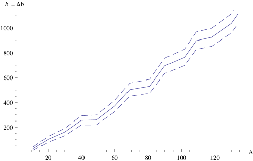
Figure 5: Quadrupole values $b$ (full line) and $b\pm\Delta b$ (dashed lines) for $\gamma=4/3$.

With $\gamma$=3/4, typical results are listed in Table II and shown in Fig. 6. Relative fluctuations $\Delta b/|b|$ decrease when $A$ increases, as should be expected, but an order of magnitude of several percent at least cannot be avoided.

A	Quadrupole	Square deviation	Relative uncertainty
9	-169/16	3647/128	0.51
22	-389/8	6019/64	0.20
28	-225/4	4095/32	0.20
38	-173/2	3067/16	0.16
50	-1185/8	17895/64	0.11
62	-1399/8	23585/64	0.11
71	-3685/16	56867/128	0.092
79	-3815/16	64945/128	0.094
86	-2205/8	36459/64	0.087
101	-5531/16	90301/128	0.077
107	-5837/16	97339/128	0.076
116	-3281/8	54247/64	0.071
129	-7973/16	125443/128	0.063

Table 2: Typical results for $\gamma=3/4$.

If spin, for electrons, and both spin and isospin are reinstated, for nucleons, keeping the same occupied levels while particle number is multiplied by $2$ and $4$, respectively, it is obvious that $\Delta b/|b|$ is divided by $\sqrt{2}$ and by $2$, respectively. Actually, for nucleons, the proton number is usually smaller than that of neutrons, and orbitals may somewhat differ, hence the exact reduction factor of $\Delta b/|b|$ will slightly differ from $2$, but this changes nothing to the fact that quantum fluctuations exist and a relative uncertainty of at least a few percent cannot be avoided.

Figure 6: Quadrupole values $b$ (full line) and $b\pm\Delta b$ (dashed lines) for $\gamma=3/4$.

3.3 Fluctuation in a constrained diagonalization

We consider in this section a one-dimentsional Hamiltonian, $H=-d^{2}/dr^{2}+v(r)$, with a double hump potential, $v=(r-1/5)^{6}/5000\,e^{-r^{2}/12}+(r/12)^{6}/8$, shown as a full line in Fig. 7.

We take the constrained Hamiltonian as ${\cal H}=H-\lambda\,r$ and diagonalize it in a subspace spanned by shifted Gaussians. While the eigenstate, $\psi_{\lambda}(r),$ shows a single wave-packet when the average value, $\left\langle r\right\rangle\equiv\left\langle\psi_{\lambda}\left|r\right|\psi_{\lambda}\right\rangle,$ sits near a minimum of $v$, an expected tunnel effect occurs when $\left\langle r\right\rangle$ sits near a maximum of $v$. There $\psi$ shows two connected packets, one at each side of the barrier, inducing a lowering of the energy. Such a bimodal (even multimodal in several extreme cases we tested) situation induces a very bad probing of the barrier. The plot of the energy, $e=\langle H\rangle$, (multiplied ten times for graphical reasons) in terms of $\langle r\rangle$ does not reflect $v(r$) in any way, see the thin full line in Fig. 8. When tunnel effects occur, fluctuations, $\Delta r=\sqrt{\left\langle r^{2}\right\rangle-\left\langle r\right\rangle^{2}},$ are dramatically larger than when a unique packet sits in a valley. The label, $\langle r\rangle$ in our case, is thus misleading. Although $\mathcal{H}$ was exactly diagonalized, constrained variation generated a bad quality representation of $v(r)$. Fig. 8 illustrates how big the uncertainty on $\langle r\rangle$ can become. Moreover, this “energy surface” turns out to be convex.

The previous models in this Section show that somewhat large quantum fluctuations of collective coordinates do exist, but the present model, in this Subsection, illustrates a new fact, namely that such fluctuations may vary along an energy surface and may influence the surface itself. A trivial way to prevent fluctuations from arbitrarily varying is to introduce a double constraint via the square, $B^{2}$, of the initial constraint operator [15]. One adjusts the second Lagrange multiplier so that the fluctuation, $\Delta b$, remains small, and, for a stable quality of the representation, reasonably constant. (Alternately one can tune the second Lagrange multiplier to ensure more or less constant and/or small enough ratios $\Delta b/|b|$.) Again with 1-D toy Hamiltonians of the form, ${\cal H}^{\prime}=-d^{2}/dr^{2}+v(r)-\lambda_{1}r+\lambda_{2}r^{2},$ or, equivalently, ${\cal H}^{\prime}=-d^{2}/dr^{2}+v(r)+\lambda_{2}(r-\lambda_{1})^{2},$ we tuned $\lambda_{2}$ into a function $\lambda_{2}(\lambda_{1})$ to enforce a unimodal situation with $\Delta r$ kept constant when $\langle r\rangle$ evolves. A sharp, stable probe of the barrier results. Convexity is then “defeated”. The true shape of $v$ is recovered [15].

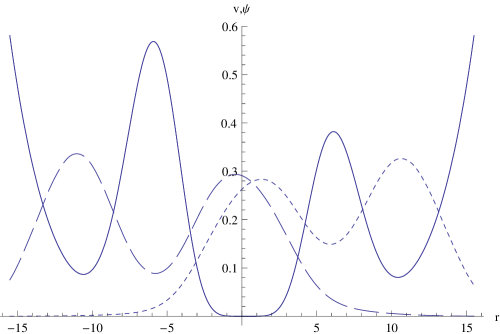
Figure 7: Toy model, 1-D potential, full curve. Tunnel effect of constrained eigenstate under left barrier, dashed curve. Same effect under right barrier, dotted curve.

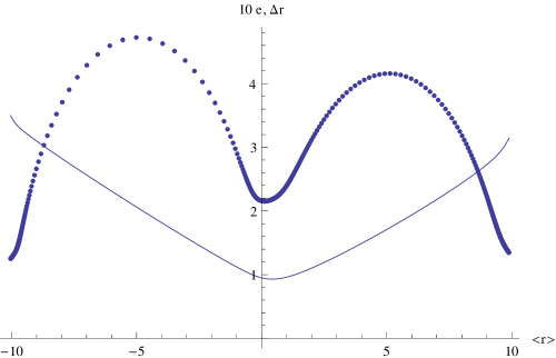
Figure 8: Same toy model. Energy curve, full line. Fluctuation curve, dots. Strong increase of $\Delta r$ when the constrained eigenstate delocalizes into two wave packets.

4 Discussion and conclusion

The present work shows that expectation values of collective coordinate operators may lead to misleading coordinates for an energy surface. Convexity is a major property of any energy surface obtained by an exact minimization of the energy under constraint(s), and may occur through tunnel effects and collective coordinate fluctuations. If an energy landscape with “saddles” is needed, such deviations from convexity contradict the requirement that the energy must transit through exact minima. The success of collective models that use a non-trivial landscape via mean field approximations is too strong to be rejected as physically and/or mathematically unsound, but its validation likely relates to further methods such as, resonating group methods [18], generator coordinate (GC) ones [19, 20], Born-Oppenheimer approximations, influence functionals [21], deconvolutions of wave packets in collective coordinate spaces [22], etc. In particular, one can argue that, while individual exact states $\psi_{\lambda}$ or mean-field ones $\phi_{\lambda}$ may carry large uncertainties for the label $b,$ such states may still provide a good global set for a GC calculation. But then the physics lies as much in non-diagonal elements $H(b,b^{\prime})$ and $N(b,b^{\prime})$ of the GC energy and overlap kernels, respectively, than in the diagonal, $e(b)\equiv H(b,b).$

Even so, except for anharmonic vibrations, where one valley is sufficient, one has to justify why concave branches can be as significant as branches obtained from exact minimizations of the energy.

Because of kinetic terms, which enforce delocalizations, a full Hamiltonian is often not well suited to ensure a good localization of the operators, $B$, a necessary condition for the exploration of an energy surface parametrized by their expectation values, $b$. Recall that, in the Born-Oppenheimer treatment of the hydrogen molecule, the proton kinetic energy operator is initially removed from the Hamiltonian, allowing the collective coordinate, namely the interproton distance, to be frozen as a zero-width parameter. Most often in nuclear, atomic, and molecular physics, such a removal is not available. Hence, such an approach may lead to “dangerous consequences”, as illustrated by Fig. 8, from the toy Hamiltonian introduced at the stage of Fig. 7. The growth of fluctuations due to tunnel effects is spectacular. Fortunately, if one forces the constrained eigenstate to retain a narrow width while the collective label runs, convexity is defeated at the profit of a reconstruction of the potential shape.

The technical devices used with success in Refs. [7, 10, 11, 12] require a further investigation of the solutions they generated. Uncertainties in the collective coordinates must be acknowledged. “Mountains” can be underestimated, as is the case when tunnel effects deplete the energy probing wave function. (A hunt for multimodal solutions would therefore be useful.) Since fluctuations are important at “phase transitions”, collective operators must be completed by their own squares, in combinations of the form, $\mathcal{K}=H-\lambda B+\mu(\lambda)B^{2}$, with $\mu(\lambda)$ adjusted to avoid wild increases of $\Delta b$ . Such operators $\mathcal{K}$ govern both a constraint and its fluctuation, but obviously differ from a double constraint form, $\mathcal{H}=H-\lambda_{1}B+\lambda_{2}B^{2}$, with two independent parameters, $\lambda_{1},\lambda_{2}$. The second derivative, $d^{2}\varepsilon/d\lambda^{2}$ contains additional terms due to $d\mu/d\lambda$ and $d^{2}\mu/d\lambda^{2}$, hence a one-dimensional path with non convex structures can be induced by $\mathcal{K}$ inside that convex two-dimensional landscape due to $\mathcal{H}$. We verified this “adjustable $B^{2}$” method with many numerical tests.

In theories using, partly at least, liquid drop models, see Ref. [23] for instance, labels $b$ are purely classical. Such theories are thus safe from the present concerns. But many other energy surfaces used in realistic situations come from mean-field constrained calculations. It remains to be tested whether their solutions, stable or metastable, carry a mechanism that diminishes the fluctuation of collective degrees of freedom. This mechanism, if it exists, deserves investigation. We conclude that a review of landscapes obtained by constrained HF or HB is in order, to analyze the role of collective coordinate fluctuations. It is clear that such surfaces deserve corrections because of likely variable widths $\Delta b$ of their collective observables, and also, obviously, because convolution effects and zero-point energies must be subtracted.

To summarize, we first found that collective operators carry significant fluctuations. We also found that fluctuations, and convexity situations, can enforce poor energy landscapes if constrained energy minimizations are used with fixed operators $B$ and fixed trial spaces. Unacceptable uncertainties, $\Delta b$, can vitiate the meaning of collective labels. We did even discover bi- or multimodality in mean field approximations. Fortunately, given the same fixed operators and trial spaces, a modest deviation from fixed constraints, namely adjustable combinations of $B$ and $B^{2},$ commuting operators indeed, allows an analysis “at fluctuations under control”, with unimodal probes of landscapes and a controlled quality of the collective representation. A puzzling question remains: is the good quality of constrained mean field solutions in the literature [10, 11] the result of a “self damping” of collective coordinate fluctuations? Are multimodal situations blocked when nuclear mass increases?

SK acknowledges support from the National Research Foundation of South Africa. BG thanks N. Auerbach for stimulating discussions and the University of Johannesburg and the Sackler Visiting Chair at the University of Tel Aviv for their hospitality during part of this work.

References

References

- [1] A. Bohr, B. R. Mottelson, Nuclear Structure, World Scientific, 1998.
- [2] J. R. Nix, W. J. Swiatecki, Studies in the liquid-drop theory of nuclear fusion, Nucl. Phys. 71 (1964) 1.
- [3] P. Bonche, Time dependent Hartree Fock calculations for heavy ion collisions, J. Physique 37 C (1976) 5.
- [4] F. Villars, Adiabatic time-dependent Hartree-Fock theory in nuclear physics, Nucl. Phys. A 285 (1977) 269.
- [5] A. Bulgac, A. Klein, N. R. Walet, G. D. Dang, Adiabatic time-dependent Hartree-Fock theory in the generalized valley approximation, Phys. Rev. C 40 (1989) 945.
- [6] K. Matsuyanagi, M. Matsuo, T. Nakatsukasa, N. Hinobara, K. Sato, Open problems in the microscopic theory of large-amplitude collective motion, J. Phys. G 37 (2010) 064018.
- [7] B. G. Giraud, J. L. Tourneux, S. K. M. Wong, Constrained Hartree-Fock calculations for a quadrupole generator coordinate, Phys. Lett. B 32 (1970) 23.
- [8] J. Ryckebusch, W. Cosyn, M. Vanhalst, Density dependence of quasifree single-nucleon knockout reactions, Phys. Rev. C 83 (2011) 054601.
- [9] T. Lesinski, Density functional theory with spatial-symmetry breaking and configuration mixing, Phys. Rev. C 89 (2014) 044305.
- [10] H. Flocard, P. Quentin, A. K. Kerman, D. Vautherin, Nuclear deformation energy curves with the constrained Hartree-Fock method, Nucl. Phys. A 203 (1973) 433.
- [11] H. Flocard, P. Quentin, D. Vautherin, M. Veneroni, A. K. Kerman, Self-consistent calculation of the fission barrier of 240Pu, Nucl. Phys. A 231 (1974) 176.
- [12] A. Staszczak, M. Stoitsov, A. Baran, W. Nazarewicz, Augmented lagrangian method for constrained nuclear density functional theory, Euro. Phys. J. A 46 (2010) 85, and references cited therein.
- [13] B. R. Barrett, B. G. Giraud, B. K. Jennings, N. Toberg, Concavity for nuclear bindings, thermodynamical functions and density functionals, Nucl. Phys. A 828 (2009) 267.
- [14] K. Neergaard, V. V. Pashkevich, S. Frauendorf, Shell energies of rapidly rotating nuclei, Nucl. Phys. A 262 (1976) 61.
- [15] B. G. Giraud, S. Karataglidis, Symmetries and fluctuations in the nuclear density functional, Physica Scripta 89 (2014) 054009.
- [16] R. Balian, From Microphysics to Macrophysics: Methods and Applications of Statistical Physics, Springer, Berlin, 2007.
- [17] B. G. Giraud, S. Karataglidis, Algebraic density functionals, Phys. Lett. B 703 (2011) 88.
- [18] K. Wildermuth, Y. C. Tang, A unified theory of the nucleus, Academic, New York, 1977.
- [19] D. L. Hill, J. A. Wheeler, Nuclear constitution and the interpretation of fission phenomena, Phys. Rev. 89 (1953) 1102.
- [20] J. J. Griffin, J. A. Wheeler, Collective motions in nuclei by the method of generator coordinates, Phys. Rev. 108 (1957) 311.
- [21] R. P. Feynman, F. L. Vernon, The theory of a general quantum system interacting with a linear dissipative system, Ann. Phys. (N.Y.) 24 (1963) 118.
- [22] B. G. Giraud, B. Grammaticos, Energy surfaces, collective potentials and collective inertia parameters, Nucl. Phys. A 233 (1974) 373.
- [23] P. Moller, A. J. Sierk, T. Ichikawa, A. Iwamoto, R. Bengtsson, H. Uhrenholt, S. Aberg, Heavy-element fission barriers, Phys. Rev. C 79 (2009) 064304.